Equilibrium temperature anisotropy and black-hole analogues

Abstract

When long-range interactions are present the usual definition of temperature implies that two systems in thermal equilibrium can be at different temperatures. This local temperature has physical significance, if the sub-systems cease to interact, each system will be at their different local temperatures. This is formally related to redshifting of temperature in general relativity. We propose experiments to test this effect which are feasible using current microfabrication techniques. It is also possible to display thermodynamical analogues to black-hole space-time.

I introduction

When a system possesses long-range interactions, many familiar notions of thermodynamics break down; the micro-canonical and canonical ensembles become inequivalent pad , there may be no stable equilibrium configuration Antanov (1962); Lynden-Bell and Wood (1968), and heat-capacities can be negative Lynden-Bell and Wood (1968); Thirring (1970) as observed in fragmenting nuclei et. al. (2000) and atomic clusters Schmidt et al. (2001). Formally, standard thermodynamics has only been proved valid when interactions are short-range, or when the long-range interactions are screened (e.g. plasmas) Lebowitz and Lieb (1969). There are few methods for studying the thermodynamics of systems with long-range interactions, although some models have been studied for special cases where the thermodynamic limit exists Dyson (1969), and understanding them outside the standard framework using Tsallis or Renyi entropy has been attempted.

Using a general formalism for studying such systems Oppenheim (2003) based on techniques used in general relativity (where the equivalence principle is exploited) – an effect was noted which we summarise and extend as follows. Consider many strongly interacting sub-systems in thermal equilibrium. Using the standard definition of temperature (defined as the local temperature), each sub-system is at a different temperature even though the entire system is at thermal equilibrium Oppenheim (2003). Clearly the standard definition does not satisfy a basic notion – that it be constant throughout the sample at equilibrium, yet it has a physical meaning – if the interaction is turned off suddenly and the sub-systems isolated, they will be at their local temperatures. The observed temperature difference when a system is broken down into its parts is a property of the system and is a function of its self-interaction. What’s more, the effect is formally related to effects found in curved space and black hole thermodynamics Oppenheim (2003). Here we show that this anisotropy of local temperature can be observed, though this requires the long-range interaction to be strong compared with the characteristic temperature of the sample. However, recent advances in microfabrication may allow experimental access to thermodynamical effects not found in macroscopic systems. An experiment to measure the break-down of temperature in quantum systems was recently proposed in Hartmann and Mahler (2005).

We review the basic formalism for analysing systems with long range interactions and then apply this to a proposed experiment. We also show that one can observe additional effects closely related to thermodynamical relations in black-hole space-times.

II Long-Range Interactions

Consider two sub-systems, with total energy $m$ of the form

$$m=E_{1}+E_{2}+G(E_{1},E_{2}),$$ (1)

where $E_{i}$ are the local (non-interacting) energies and $G(E_{1},E_{2})$ is some interaction potential (which may include self-interacting terms). As an example, we consider the interaction of two clusters of classical spins in local magnetic fields $b_{1}$ and $b_{2}$, with spin-spin interaction

$$m=b_{1}e_{1}+b_{2}e_{2}-J_{1}e_{1}^{2}/2-J_{2}e_{2}^{2}/2-J_{12}e_{1}e_{2},$$ (2)

where $e_{1}$ and $e_{2}$ are the spin-excesses of each cluster $e_{i}=n_{i}^{\uparrow}-n_{i}^{\downarrow}$, ($n_{i}^{\uparrow}$ and $n_{i}^{\downarrow}$ being the number of up and down spins respectively of cluster $i=1,2$), $J_{i}$ are intra-cluster couplings, and $J_{12}$ is the inter-cluster coupling. Such an interaction arises from a standard interaction between spins of the form

$$m=\sum b_{1}\sigma_{1}^{j}+\sum b_{2}\sigma_{2}^{k}-\sum_{lm}\sum_{i,i^{\prime}=1,2}J_{ii^{\prime}}^{kl}\sigma_{i}^{k}\sigma_{i}^{\prime l}$$ (3)

with the spins of cluster $i$ being $\sigma_{i}^{j}$. For small clusters, the interaction within each cluster can be approximately the same for all spins, not just nearest neighbour, i.e. $J_{11}^{kl}=J_{1},J_{22}^{kl}=J_{2}$, and the interaction between each cluster is approximately uniform over each cluster i.e. $J_{12}^{kl}=J_{12}$. We then drop constant terms to obtain Eq. (2). Gravity is another common example of such an interaction, where the potential term depends on the local energies (masses) of each system.

One can define the temperature of one of the clusters (the system ${\cal S}$), by making the other system very large (the reservoir ${\cal R}$). If the total energy $m$ is fixed, in this limit the probability that the system has energy $E_{\cal S}$ is given by Oppenheim (2003)

$$p(E_{\cal S})dE_{\cal S}=\sum_{E}\Omega_{S}(E_{\cal S})\Omega_{R}(E)e^{-E_{\cal S}\beta_{E}}dE_{\cal S}/Z_{m}$$ (4)

where the sum is taken over all $E=E_{\cal R}+E_{\cal S}$ consistent with total energy $m=E+G(E_{\cal S},E_{\cal R})$ and

$$Z_{m}=\int_{m}dE_{\cal S}\Omega_{S}(E_{\cal S})e^{S_{\cal R}(E_{\cal R})}$$ (5)

i.e. $Z_{m}$ is the total number of states at fixed total energy $m$. We then define the inverse temperature $\beta_{E}$ in the usual manner in terms of the local extensive entropy

$$\beta_{E}\equiv\frac{\partial S_{\cal R}(E_{\cal R})}{\partial E_{\cal R}}\,\,\,\,$$ (6)

We shall refer to $\beta_{E}$ as the local temperature. The motivation for using this term comes from general relativity.

Note that the temperature of the system is defined in terms of the derivative of the reservoir’s entropy. In the non-interacting case, no issues arise from this definition: if two systems are in thermal contact in the microcanonical ensemble, then $\frac{\partial S_{\cal S}(E_{\cal S})}{\partial E_{\cal S}}\simeq\frac{\partial S_{\cal R}(E)}{\partial E}$. This is also true when the reservoir has no long-range interactions, or when the division of a single system into a reservoir and smaller system is purely formal (as we will see from symmetry considerations). In general however, this is not necessarily true – a point which will be discussed shortly. One therefore should keep in mind that the temperature is a property of a reservoir – it gives the distribution associated with a smaller system in contact with it. Finally, note that the local temperature, as defined, is a function of $E$, we make this explicit by writing $\beta_{E}$. There will be different “temperatures” depending on the value of $E$ the entire system is found in.

Let us now show that at equilibrium, a system can have an anisotropy in local temperature. Here we consider a slightly different situation and derivation than in Oppenheim (2003). For concreteness, one could consider a system, as above, composed of two clusters as above labelled $1$ and $2$. For fixed $E_{1}$ and $E_{2}$, the spin excesses of each cluster are fixed, thus their respective entropy is also fixed and given by

$$S_{i}(E_{i})=-n_{i}^{\uparrow}\log\frac{n_{i}^{\uparrow}}{n_{i}^{\uparrow}+n_{i}^{\downarrow}}-n_{i}^{\downarrow}\log\frac{n_{i}^{\downarrow}}{n_{i}^{\uparrow}+n_{i}^{\downarrow}}$$ (7)

and since each entropy is determined only by the spin excess, the total entropy is additive, i.e. the number of states accessible to two systems is given by the number of states accessible to one system, times the number of states accessible to the other. I.e.

$$\Omega_{12}(E_{1},E_{2})=\Omega_{1}(E_{1})\Omega_{2}(E_{2})$$ (8)

where $\Omega_{12}$ is the total number of states of the combined system, and $\Omega_{i}$ is the number of states accessible to system $i$ (the entropies of each system are just $S_{i}(E_{i})=\log\Omega_{i}(E_{i})$). Additivity of entropy holds because we will find that we only need it at each value of $E_{1},E_{2}$ and in this case, the entropy is additive in many systems because often the only correlations in a system are related to correlations in energy. We can thus consider more general systems with additive entropies (when conditioned on local energy). We now consider these two systems in contact with a reservoir ${\cal R}$ at fixed total energy $m=E_{1}+E_{2}+E_{\cal R}+G(E_{1},E_{2})$ and again taking the total local energy as $E=E_{1}+E_{2}+E_{R}$. The probability that the two systems have energy $E_{1}$ and $E_{2}$ for given local energy $E$ is $\Omega_{1}(E_{1})\Omega_{2}(E_{2})\Omega_{R}(E_{R})/Z_{E}$, and the probability that the local energy is $E$ is denoted by $p(E)=Z_{E}/Z_{m}$, with the partition functions $Z_{m}=\sum_{E_{1},E_{2},E}\Omega_{1}(E_{1})\Omega_{2}(E_{2})\Omega_{R}(E_{R})$ at fixed $m$ and $Z_{E}=\sum_{E_{1},E_{2}}\Omega_{1}(E_{1})\Omega_{2}(E_{2})\Omega_{R}(E_{R})$ at fixed $E$. Then the probability that system $1$ has energy $E_{1}$ is

$$p_{1}(E_{1}) =\sum_{E,E_{2}}p(E_{1},E_{2}|E)Z_{E}/Z_{m}$$

$$=\sum_{E,E_{2}}\Omega_{1}(E_{1})\Omega_{2}(E_{2})\Omega_{R}(E_{R})/Z_{m}$$ (9)

$$\simeq\frac{\Omega_{1}(E_{1})}{Z_{m}}e^{S_{R}(m)-\beta_{o}E_{1}}\sum_{E,E_{2}}\Omega_{2}(E_{2})e^{-\beta_{o}(E_{2}+G(E_{1},E_{2}))}$$

where we have used the approximation that $E_{\cal R}\gg E_{1}+E_{2}+G(E_{1},E_{2})$ to expand $S_{R}$ around $m$ with the inverse global temperature defined as $\beta_{o}\equiv\partial S_{R}(m)/\partial m$. Since $m$ is held fixed, an absence of interaction $G(E_{1},E_{2})$ would give the usual fact that $p_{1}(E_{1})$ will be proportional to $\Omega_{1}(E_{1})e^{-\beta_{o}E_{1}}$, and symmetrically for $p_{2}(E_{2})$ – thus the systems will be at equal temperature. Here, we have the additional sum over $E$ and the factor due to the interaction term, which makes the distribution of system $1$ and system $2$ asymmetric. Expanding $G(E_{1},E_{2})$ around $(E_{1},E_{2})=(\bar{E}_{1},\bar{E}_{2})$ the average energies, gives

$$p(E_{1})\propto\Omega_{1}(E_{1})e^{-(1+\frac{\partial G(\bar{E}_{1},\bar{E}_{2})}{\partial\bar{E}_{1}})\beta_{o}E_{1}}$$ (10)

which looks like a canonical distribution. By symmetry, each system thus behaves as if it has an inverse temperature

$$\beta_{i}=(1+\frac{\partial G(\bar{E}_{1},\bar{E}_{2})}{\partial\bar{E}_{i}})\beta_{o}$$ (11)

One can calculate that this local temperature matches the standard definition of temperature given by Eq. (6) and we thus see that there is a temperature anisotropy whenever $\partial G(\bar{E}_{1},\bar{E}_{2})/\partial\bar{E}_{2}\neq\partial G(\bar{E}_{1},\bar{E}_{2})/\partial\bar{E}_{1}$

Let us now understand the physical meaning of this local temperature. Eq. (4) gives the probability distribution of a system ${\cal S}$ in terms of the local temperature $\beta$, and the local energy $E_{\cal S}$. However, the local energy is not a conserved quantity, and does not contain the interacting term. To see what the locally conserved energy is, we can expand $m$ to first order $m(E_{1},E_{2})\simeq m(\bar{E}_{1},\bar{E}_{2})+\frac{\partial m}{\partial E_{1}}(E_{1}-\bar{E}_{1})+\frac{\partial m}{\partial E_{2}}(E_{2}-\bar{E}_{2})$. Since constant terms can be ignored, $E_{o}^{i}\equiv\frac{\partial m}{\partial E_{i}}E_{i}$ can be identified with the energy of each system in the presence of the mean field due to the other interacting systems and is $(1+\frac{\partial G(\bar{E}_{1},\bar{E}_{2})}{\partial\bar{E}_{i}})E_{i}$. In the case of a single system and reservoir, this energy is $E_{o}\equiv E_{\cal S}\frac{\partial m}{\partial E_{\cal S}}$ and serves to tell us how we should define the locally conserved energy. As is expected for a non-extensive system, the quantity is also non-additive, but, as with the local temperature, will correspond with what happens in general relativity.

$E_{o}$ is also a function of $E$ but we will not write this explicitly. With respect to energy levels $E_{o}$, each system acts approximately as if it is at inverse temperature $\beta_{o}$ (although in actual fact it is a mixture of temperatures Oppenheim (2003)). We can think of $E_{o}$ as the effective energy, i.e. it is the energy of the system in the presence of interaction with another system, and $\beta_{o}$ can be thought of as the closest thing one has to a physical temperature – looking at Eq. (11) we see that the global inverse temperature $\beta_{o}$ will be equal for both systems. Note however, that the global temperature is not an intensive quantity.

If the interaction term is suddenly “turned off”, (one can imagine that the spins are suddenly separated so that they no longer interact), then the energy that is ascribed to each energy level is no longer $E_{o}^{i}$, but rather its local energy $E_{1}$ or $E_{2}$. If the change happens extremely quickly then the overall state of the system will not change. Since

$$\beta_{i}E_{i}=\beta_{o}E_{o}^{i}$$ (12)

and the new energy of each system is now $E_{i}$, the measured temperatures will be $\beta_{i}$ – the local temperature. In these systems, the local temperature becomes the physical one when the interaction is turned off, which is analogous to the fact that in general relativity, the local temperature is the physical one measured by free-falling observers (for whom the gravitational interaction is “turned off”).

Using the two coupled Ising models of Eq. (2) we would get a temperature difference of

$$\beta_{2}=\beta_{1}\frac{1-J_{12}e_{1}/b_{2}-J_{2}e_{2}/b_{2}}{1-J_{12}e_{2}/b_{1}-J_{1}e_{1}/b_{1}}\,\,\,\,.$$ (13)

Now if initially these two systems (or clusters), are far apart, and at equal global temperature, one cannot push them together both adiabatically and isothermally (constant global temperature) as is possible in the non-interacting case. This can be seen from Eq. (12). Moving the systems together adiabatically requires keeping $E_{o}\beta_{o}$ fixed, but since $E_{o}$ changes when $J_{12}$ becomes significant, one cannot keep $\beta_{o}$ constant. By recalculating $E_{o}$ one can therefore calculate the new global temperature. We see therefore that the global temperature is not an intensive quantity.

III Black-hole on a benchtop

To obtain an analogue of a black-hole, we consider a single cluster of spins with long-range self-interaction. This can be obtained by setting $h_{2}=J_{2}=J_{12}=0$. This gives a relation between the local and global temperature of

$$\beta=\pm\beta_{o}\sqrt{1-\frac{2J_{2}m}{h^{2}}}\,\,\,\,.$$ (14)

The positive solution looks exactly like the relationship between global and local temperature in the Schwarzschild black-hole space-time due to redshifting, if we set the radius $r=h^{2}$ and equate the spin-spin coupling with Newton’s constant $J_{1}=G$. Here $\beta_{o}$ is the temperature at infinity, while $\beta$ would be the local temperature measured by an observer sitting close to the black-hole horizon. In the analogue, the horizon is real – for fixed $m$, there is no value of spin-excess which allows $r<2Gm$ i.e. $m>h^{2}/2J_{1}$. There are also many similarities between this analogue and a black hole in terms of the way the entropy and energy behave, and we refer the reader to Oppenheim (2003, 2002) for details.

IV Experimental Realisation

Ideally, we would like to study these phenomena in complex macroscopic systems. However these usually do not possess a strong enough long-range interaction to produce an appreciable effect, hence it is necessary to go to small systems where the the coupling between sub-systems can be comparable to the local energies and low temperatures are easier to achieve.

The simplest system to study that of two spin clusters coupled via an Ising-like interaction,

$$H=\vec{b}_{1}\cdot\vec{\sigma}^{1}+\vec{b}_{2}\cdot\vec{\sigma}^{2}+\frac{J}{2}\sigma_{z}^{1}\otimes\sigma_{z}^{2}$$ (15)

where $\vec{b}_{i}$ are local magnetic fields and $J$ is the interaction energy between the two clusters. We can map this system to a pair of pseudo-spins such as double quantum dots with a excess electrons whose localisation in one or the other dot defines the pseudo-spin vector (Fig. 1 or Fig. 2). A single electron transistor measures the total charge excess in one dot or the other.

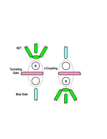
Figure 1: Coupled double quantum dot (DQD) system constructed from donor phosphorus atoms in silicon with $20nm$ vertical and $30nm$ lateral separation. Each left and right DQD pair is initialised with one electron shared between the two dots. The local Hamiltonians can be controlled by electrodes affecting the tunnelling rate and bias between the two dots. The interaction is of the Ising type ($J=2.9meV$) and single electron transistors (SETs) measure the localisation of the electrons to the upper or lower dots of each pair.

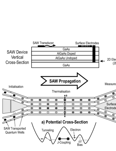
Figure 2: Surface acoustic wave (SAW) device. The SAW created by an interdigital transducer produces a sinusoidal piezoelectric field in the direction of propagation which, together with surface electrode located above a 2DEG, create a pattern of moving quantum wells which can be manipulated by static voltages. The advantage of this configuration is that the interacting sub-systems can be separated before measurement of their respective populations. Correlated current readout measures the population in the position basis.

To implement the separation of the two sub-systems before measurement, the device in Fig. 2 could be used. A surface acoustic wave (SAW), produced in a piezoelectric material by an inter-digital transducer driven by a microwave generator, induces a travelling sinusoidal electric field in a 2-dimensional electron gas (2DEG) situated just below the surface of a modulation-doped GaAs-AlGaAs semiconductor. Bias electrodes on the surface of the device deplete the 2DEG of conduction electrons on the region of the system.

By suitable electrode potentials at the entrance of the system, an exact number of electrons can be transported in moving quantum dots, along quasi-1D quantum channels (defined by surface electrodes) through the device. Double well potentials can be created with a specified number of electrons in each, and by using suitable electrode geometry, made to interact via an Ising coupling. Travelling along a sufficiently long channel, the sub-systems are allowed to thermalise, after which the two sub-systems are rapidly separated and read-out by simply measuring the current via Ohmic contacts.

Figure 3: A plot of the temperatures of two interacting sub-systems consisting of several electrons with Coulomb exchange energy.

- (1) For a good review, see for example T. Padmanabhan, Phys Rep, 188, 285-362 (1990).
- Antanov (1962) V. A. Antanov, Vest. Leningr. Gos. Univ: Mat. Mekh. Astron. 7, 135 (1962).
- Lynden-Bell and Wood (1968) D. Lynden-Bell and R. Wood, MNRAS 128, 495 (1968).
- Thirring (1970) W. Thirring, Z. Phys 235, 339 (1970).
- et. al. (2000) M. A. et. al., Phys. Lett. B 473, 219 (2000).
- Schmidt et al. (2001) M. Schmidt, R. Kusche, T. Hippler, J. Donges, W. Kronmuller, B. von Issendorff, and H. Haberland, Phys. Rev. Lett. 86, 1191 (2001).
- Lebowitz and Lieb (1969) J. Lebowitz and E. Lieb, Phys. Rev. Lett. 22, 631 (1969).
- Dyson (1969) F. Dyson, Commun. Math. Phys. 12, 91 (1969).
- Oppenheim (2003) J. Oppenheim, Phys. Rev. E 68, 016108 (2003), eprint gr-qc/0212066.
- Hartmann and Mahler (2005) H. Hartmann and G. Mahler, Europhys. Lett 70, 579 (2005).
- Oppenheim (2002) J. Oppenheim, Phys. Rev. D 65, 024020 (2002), eprint gr-qc/0105101.