The Cosmology of $f(R)$ Gravity in the Metric Variational Approach

Abstract

We consider the cosmologies that arise in a subclass of $f(R)$ gravity with $f(R)=R+\mu^{2n+2}/(-R)^{n}$ and $n\in(-1,0)$ in the metric (as opposed to the Palatini) variational approach to deriving the gravitational field equations. The calculations of the isotropic and homogeneous cosmological models are undertaken in the Jordan frame and at both the background and the perturbation levels. For the former, we also discuss the connection to the Einstein frame in which the extra degree of freedom in the theory is associated with a scalar field sharing some of the properties of a ’chameleon’ field. For the latter, we derive the cosmological perturbation equations in general theories of $f(R)$ gravity in covariant form and implement them numerically to calculate the cosmic-microwave-background temperature and matter-power spectra of the cosmological model. The CMB power is shown to reduce at low $l$’s, and the matter power spectrum is almost scale-independent at small scales, thus having a similar shape to that in standard general relativity. These are in stark contrast with what was found in the Palatini $f(R)$ gravity, where the CMB power is largely amplified at low $l$’s and the matter spectrum is strongly scale-dependent at small scales. These features make the present model more adaptable than that arising from the Palatini $f(R)$ field equations, and none of the data on background evolution, CMB power spectrum, or matter power spectrum currently rule it out.

I Introduction

Theories of $f(R)$ gravity as an explanation of the dark energy problem have attracted much recent attention. These theories are of particular interest since $f(R)$ modifications to general relativity (GR) appear naturally in the low-energy effective actions of the quantum gravity and the quantization of fields in curved spacetime. These theories are also conformally related to GR with a self-interacting scalar field Barrow (1988) and both the early time inflation and the late-time acceleration of the universe could be resulted by a single mechanism in such theories. In refs. Carroll (2005); Easson (2005), the specific model in which the correction is a polynomial of $R^{2},R^{ab}R_{ab}$ and $R^{abcd}R_{abcd}$ is considered and the analysis there shows that late-time accelerating attractor solutions exist. Meanwhile, models with $R,R^{ab}R_{ab}$ corrections are discussed within the Palatini approach Vollick (2003); Allemandi (2004, 2004, 2005), in which the field equations are second order, and similar acceleration solutions are found. The Palatini-$f(R)$ theory of gravitation was then tested using various cosmological data such as Supernovae (SN), Cosmic Microwave Background (CMB) shift parameter, baryon oscillation and Big Bang Nucleosynthesis (BBN), in Capozziello (2006); Amarzguioui (2006); Sotiriou (2006); Fay (2007); Borowiec (2006). Recently, constraints from CMB and matter power spectra have also been given in Koivisto (2006); Li (2006, 2006). These constraints (especially that from the matter power spectrum) successfully exclude most of the parameter space, making the model indistinguishable from the standard $\Lambda\mathrm{CDM}$ in practice.

Turning to the metric $f(R)$ gravity theories, the field equations become fourth order and more difficult to handle Barrow (1983). Until now, much attention has been focused on the solar system tests of the theory and the existing results appear to exclude a viable $f(R)$ cosmological model that leads to the current cosmic accelerating expansion (see, for example, Chiba (2003); Erickcek (2006); Navarro (2006); Olmo (2005, 2005, 2006) and references therein; also see Zhang (2007) and references therein for arguments against these). Regardless of these local considerations, however, we can look at the cosmological behavior of the theory in order to arrive at an independent test. The cosmological constraints on $f(R)$ gravity is relevant also because one can simply imagine that the baryons do not see the modifications to GR (a possibility suggested in Amendola (2006)) evades the solar system tests in a somewhat artificial way), or transform to the Einstein frame and consider a scalar field model mathematically equivalent to the Jordan frame $f(R)$ gravity Capozziello (2006), but with the scalar field coupling only to the dark matter. For further discussion of the cosmology of the $f(R)$ dark energy models see, for example, Odintsov (2006); Mena (2006); Fay (2007) and references therein.

In a recent study, Amendola (2006), the authors find that the class of Friedmann cosmological models arising in a theory with $f(R)=R+\mu^{2(n+1)}/(-R)^{n}$ and $n>0$ (note the difference from their original paper because of our sign convention, $R<0$), which was thought to lead to the late-time acceleration because the correction term to GR becomes significant at late times, cannot reproduce the matter-dominated era of conventional cosmology (yielding $a\propto t^{1/2}$ rather than $a\propto t^{2/3}$ where $a$ is the scale factor and $t$ the cosmic time) and so will be ruled out by measurements of the redshift distance (see also Fairbairn (2007)). In this work they do not consider the case of $-1<n<0$ which is able to give a standard matter-dominated era, as we show below. In a later work, Amendola (2006), these authors consider the cosmological viabilities of general $f(R)$ models and have included this possibility.

Since there are few known models with simple forms of $f(R)$ having the capability to consistently describing the whole evolutionary history of the universe (see however Comment (2007) for a discussion on this), we will also consider the perturbation evolutions of the model. To this end we derive the covariant and gauge invariant perturbation equations and put them into the public CAMB code Lewis (2000) in order to obtain the CMB and matter power spectra. Note that the dynamics of perturbations for $f(R)$ gravity have also been considered in Song (2006); Bean (2006). In Song (2006) the background expansion is fixed to match $\Lambda\mathrm{CDM}$ while in Bean (2006) two specified models are considered which do not give standard matter-dominated eras and the calculation is done in the Einstein frame; thus both analyses differ from the work reported here.

This paper is organised as the following: in Section II we briefly introduce the cosmological model and list the background and perturbation evolution equations that are needed in the numerical calculation. In Section III we solve for the background evolution of the model numerically, and incorporate the perturbations equations into CAMB in order to calculate the CMB and matter power spectra. The discussion and conclusions are then presented in Section IV. Throughout this work we will set $c=$ $\hslash=1$ and only consider the case of a spatially flat universe filled with photons, baryons, cold dark matter (CDM) and three species of effectively massless neutrinos.

II Field Equations in f(R) Gravity

In this section we very briefly summarise the main ingredients of $f(R)$ gravity in metric approach, and list the general perturbation equations that govern the dynamics of small inhomogeneities in this theory.

II.1 The Generalised Einstein Equations

The starting point for the metric-$f(R)$ gravity is the Einstein-Hilbert action,

$$S = \int d^{4}x\sqrt{-g}\left[\frac{1}{2\kappa}f(R)+\mathcal{L}_{m}\right],$$ (1)

in which $\kappa=8\pi G$ with $G$ being the gravitational constant and $R=R(g_{ab})$ is the Ricci scalar. Varying the action with respect to the metric $g_{ab}$ gives the modified Einstein equations

$$FR_{ab}-\frac{1}{2}g_{ab}f(R)+(g_{ab}\nabla^{c}\nabla_{c}-\nabla_{a}\nabla_{b})F = \kappa T_{ab},\ \$$ (2)

where $F=F(R)\equiv\partial f(R)/\partial R$ and $T_{ab}$ is the energy-momentum tensor. The trace of Eq. (2) reads

$$FR-2f+3\nabla^{c}\nabla_{c}F = \kappa T,$$ (3)

with $T_{a}^{a}\equiv T=\rho-3p$. Let us call this the structural equation, which relates $R$ (or $F$) directly to the energy components in the universe. However, the term $\nabla^{c}\nabla_{c}F$ enters here which makes the equation a dynamical rather than algebraic one. Recall, in contrast, that in the Palatini $f(R)$ gravity the metric $g_{ab}$ and connection $\Gamma^{a}_{bc}$ are treated as independent variables with $R=R(g_{ab},\Gamma^{a}_{bc})$; the variation of the action is taken with respect to both of these two variables with the resulting field equations being second order and the structural equation simply an algebraic relation. Now we can also make a conformal transformation,

$$\tilde{g}_{ab} = e^{2\omega}g_{ab},$$ (4)

from the original Jordan frame to the Einstein frame (the tilded quantities are the Einstein frame ones from here on), in which we obtain the following action for the metric $f(R)$ gravity:

$$\tilde{S} = \int d^{4}x\sqrt{-\tilde{g}}\left[-\frac{\tilde{R}(\tilde{g})}{2\kappa}-\frac{(\tilde{\nabla}\varphi)^{2}}{2}-V(\varphi)+\tilde{\mathcal{L}}_{m}\right].\ \ \$$ (5)

In Eq. 5, we have defined a new scalar field $\varphi\equiv\sqrt{6}\omega/\kappa\equiv\sqrt{3/2\kappa}\ln F$ and its potential $V\equiv(f-FR)/2\kappa F^{2}$. Quantities in the Jordan and Einstein frames are related to each other by Amendola (2006)

$$\tilde{\rho}=\rho e^{-4\omega},\tilde{p}=pe^{-4\omega},d\tilde{t}=e^{\omega}dt,\tilde{a}=e^{\omega}a.$$ (6)

We see that in the Einstein frame the scalar field couples minimally to gravity but couples conformally to matter, and that the generality in the functional choice of $f(R)$ manifests itself in the generality of the potential $V(\varphi)$.

Since we implement our measurements in the Jordan frame, we shall treat the Jordan frame metric $g_{ab}$ as the physical one. Hence the difference between $f(R)$ gravity and GR ($f(R)=R$) can be understood as a change in the way that the spacetime curvature, and thus the physical Ricci tensor $R_{ab},$ responds to the distribution of matter.

II.2 The Perturbation Equations

The perturbation equations in general theories of $f(R)$ gravity derived in this section which uses the method of $3+1$ decomposition Challinor (1999); Lewis (2000). For more details, we refer the reader to these references and only briefly outline its main ingredients before listing out results.

The main idea of $3+1$ decomposition is to make spacetime splits of physical quantities with respect to the 4-velocity $u^{a}$ of an observer. The projection tensor $h_{ab}$ is defined as $h_{ab}=g_{ab}-u_{a}u_{b}$ which can be used to obtain covariant tensors perpendicular to $u$. For example, the covariant spatial derivative $\hat{\nabla}$ of a tensor field $T_{d\cdot\cdot\cdot e}^{b\cdot\cdot\cdot c}$ is defined as

$$\hat{\nabla}^{a}T_{d\cdot\cdot\cdot e}^{b\cdot\cdot\cdot c} \equiv h_{i}^{a}h_{j}^{b}\cdot\cdot\cdot\ h_{k}^{c}h_{d}^{r}\cdot\cdot\cdot\ h_{e}^{s}\nabla^{i}T_{r\cdot\cdot\cdot s}^{j\cdot\cdot\cdot k}.$$ (7)

The energy-momentum tensor and covariant derivative of 4-velocity are decomposed respectively as

$$T_{ab} = \pi_{ab}+2q_{(a}u_{b)}+\rho u_{a}u_{b}-ph_{ab},$$ (8)

$$\nabla_{a}u_{b} = \sigma_{ab}+\varpi_{ab}+\frac{1}{3}\theta h_{ab}+u_{a}A_{b}.$$ (9)

In the above, $\pi_{ab}$ is the projected symmetric trace-free (PSTF) anisotropic stress, $q_{a}$ the vector heat flux vector, $p$ the isotropic pressure, $\sigma_{ab}$ the PSTF shear tensor, $\varpi_{ab}=\hat{\nabla}_{[a}u_{b]}$, the vorticity, $\theta=\nabla^{c}u_{c}=3\dot{a}/a$ ($a$ is the mean scale factor) the expansion scalar, and $A_{b}=\dot{u}_{b}$ the acceleration; the overdot denotes time derivative expressed as $\dot{\phi}=u^{a}\nabla_{a}\phi$, brackets mean antisymmetrisation, and parentheses symmetrization. The normalization is chosen as $u^{a}u_{a}=1$.

Decomposing the Riemann tensor and making use of the modified Einstein equations, Eq. (2) , we obtain, after linearization, five constraint equations

$$0 = \hat{\nabla}^{c}(\varepsilon_{\ \ cd}^{ab}u^{d}\varpi_{ab});$$ (10)

$$\frac{\kappa q_{a}}{F} = \frac{\theta\hat{\nabla}_{a}F}{3F}-\frac{\hat{\nabla}_{a}\dot{F}}{F}-\frac{2\hat{\nabla}_{a}\theta}{3}+\hat{\nabla}^{b}\sigma_{ab}+\hat{\nabla}^{b}\varpi_{ab};\ \ \$$ (11)

$$\mathcal{B}_{ab} = \left[\hat{\nabla}^{c}\sigma_{d(a}+\hat{\nabla}^{c}\varpi_{d(a}\right]\varepsilon_{b)ec}^{\ \ \ \ d}u^{e};$$ (12)

$$\hat{\nabla}^{b}\mathcal{E}_{ab} = \frac{1}{2F}\kappa\left[\hat{\nabla}^{b}\pi_{ab}+\left(\frac{2}{3}\theta+\frac{\dot{F}}{F}\right)q_{a}+\frac{2}{3}\hat{\nabla}_{a}\rho\right]$$ (13)

$$-\frac{1}{2F^{2}}\left[\kappa(\rho+p)\hat{\nabla}_{a}F-\dot{F}\hat{\nabla}_{a}\dot{F}+\ddot{F}\hat{\nabla}_{a}F\right];$$

$$\hat{\nabla}^{b}\mathcal{B}_{ab} = \frac{1}{2F}\kappa\left[\hat{\nabla}_{c}q_{d}+(\rho+p)\varpi_{cd}\right]\varepsilon_{ab}^{\ \ cd}u^{b}.$$ (14)

Here, $\varepsilon_{abcd}$ is the covariant permutation tensor, $\mathcal{E}_{ab}$ and $\mathcal{B}_{ab}$ are respectively the electric and magnetic parts of the Weyl tensor $\mathcal{W}_{abcd}$, given respectively through $\mathcal{E}_{ab}=u^{c}u^{d}\mathcal{W}_{acbd}$ and $\mathcal{B}_{ab}=-\frac{1}{2}u^{c}u^{d}\varepsilon_{ac}^{\ \ ef}\mathcal{W}_{efbd}$.

In addition, we obtain seven propagation equations:

$$\dot{\rho}+(\rho+p)\theta+\hat{\nabla}^{a}q_{a} = 0;$$ (15)

$$\dot{q_{a}}+\frac{4}{3}\theta q_{a}+(\rho+p)A_{a}-\hat{\nabla}_{a}p+\hat{\nabla}^{b}\pi_{ab} = 0;$$ (16)

$$\dot{\theta}+\frac{1}{3}\left[\theta-\frac{3\dot{F}}{F}\right]\theta-\hat{\nabla}^{a}A_{a}$$

$$-\left[\frac{\hat{\nabla}^{2}F}{F}-\frac{\kappa\rho}{F}-\frac{f}{2F}\right] = 0;$$ (17)

$$\dot{\sigma}_{ab}+\frac{2}{3}\left[\theta+\frac{3\dot{F}}{4F}\right]\sigma_{ab}-\hat{\nabla}_{\langle a}A_{b\rangle}$$

$$+\mathcal{E}_{ab}+\frac{1}{2F}\kappa\pi_{ab}+\frac{1}{2F}\hat{\nabla}_{\langle a}\hat{\nabla}_{b\rangle}F = 0;$$ (18)

$$\dot{\varpi}+\frac{2}{3}\theta\varpi-\hat{\nabla}_{[a}A_{b]} = 0;$$ (19)

$$\frac{1}{2F}\kappa\left[\dot{\pi}_{ab}+\left(\frac{1}{3}\theta-\frac{3\dot{F}}{2F}\right)\pi_{ab}\right]$$

$$-\frac{1}{2F}\kappa\left[(\rho+p)\sigma_{ab}\ +\hat{\nabla}_{\langle a}q_{b\rangle}\right]$$

$$-\frac{3\dot{F}}{4F^{2}}\hat{\nabla}_{\langle a}\hat{\nabla}_{b\rangle}F-\frac{3\dot{F}^{2}}{4F^{2}}\sigma_{ab}$$

$$-\left[\dot{\mathcal{E}}_{ab}+\left(\theta+\frac{\dot{F}}{2F}\right)\mathcal{E}_{ab}-\hat{\nabla}^{c}\mathcal{B}_{d(a}\varepsilon_{b)ec}^{\ \ \ \ d}u^{e}\right] = 0;$$ (20)

$$\dot{\mathcal{B}}_{ab}+\left(\theta+\frac{\dot{F}}{2F}\right)\mathcal{B}_{ab}+\hat{\nabla}^{c}\mathcal{E}_{d(a}\varepsilon_{b)ec}^{\ \ \ \ d}u^{e}$$

$$+\frac{1}{2F}\kappa\hat{\nabla}^{c}\mathcal{\pi}_{d(a}\varepsilon_{b)ec}^{\ \ \ \ d}u^{e} = 0,$$ (21)

where the angle bracket means taking the trace-free part of a quantity.

Besides the above equations, it is useful to express the projected Ricci scalar $\hat{R}$ into the hypersurfaces orthogonal to $u^{a}$ as

$$\hat{R} \doteq \frac{\kappa(\rho+3p)-f}{F}-\frac{2}{3}\theta^{2}+\frac{1}{F}(\dot{F}\theta+3\ddot{F})+\frac{\hat{\nabla}^{2}F}{F}.$$ (22)

The spatial derivative of the projected Ricci scalar, $\eta_{a}\equiv\frac{1}{2}a\hat{\nabla}_{a}\hat{R}$, is then given as

$$\eta_{a} = \frac{a}{F}\kappa\hat{\nabla}_{a}\rho+\frac{a}{F}\left[\dot{\theta}+\frac{1}{3}\theta^{2}\right]\hat{\nabla}_{a}F-\frac{2a}{3}\left[\theta+\frac{3\dot{F}}{2F}\right]\hat{\nabla}_{a}\theta$$ (23)

$$-\frac{a}{F}\theta\hat{\nabla}_{a}\dot{F}-\frac{a}{F}\hat{\nabla}_{a}\hat{\nabla}^{2}F,$$

and its propagation equation by

$$\dot{\eta}_{a}+\frac{2\theta}{3}\eta_{a} = -\frac{a}{3F}\theta\hat{\nabla}_{a}\hat{\nabla}^{2}F-\left[\frac{\dot{F}}{F}+\frac{2}{3}\theta\right]a\hat{\nabla}_{a}\hat{\nabla}\cdot A$$ (24)

$$-\frac{a}{F}\kappa\hat{\nabla}_{a}\hat{\nabla}\cdot q-\frac{a}{F}\hat{\nabla}_{a}(\hat{\nabla}^{2}F)^{\cdot}.$$

As we are considering a spatially flat universe, the spatial curvature must vanish on large scales which means that $\hat{R}=0$. Thus, from Eq. (22), we obtain

$$\frac{1}{F}\kappa(\rho+3p)-\frac{2}{3}\theta^{2}-\frac{f}{F}+\frac{\dot{F}}{F}\theta+\frac{3}{F}\ddot{F} = 0.$$ (25)

This is just one of the modified Friedmann equations of the metric $f(R)$ gravity, and the other modified background equations (the other Friedmann equation and the energy-conservation equation) can be obtained by taking the zero-order parts of Eqs. (II.2, 15), as

$$\dot{\theta}+\frac{1}{3}\left[\theta-\frac{3\dot{F}}{F}\right]\theta+\frac{\kappa\rho}{F}+\frac{f}{2F} = 0;$$ (26)

$$\dot{\rho}+(\rho+p)\theta = 0.$$ (27)

It is easy to check that when $f(R)=R$, we have $F=1$ and these equations reduce to those of GR.

To conclude this section, we want to point out another way to derive the above perturbation equations. It follows by treating the new contributions in the Einstein equation from the $f(R)$ gravity modification as an additional effective energy momentum tensor Hwang (1990). In this way one can write

$$G_{ab} = \kappa\bar{T}_{ab}$$

$$= \frac{1}{F}\kappa T_{ab}+\frac{1}{F}\nabla_{a}\nabla_{b}F-\frac{1}{2F}(f+\kappa T-\nabla^{2}F)g_{ab},$$

where an overbar represents the total effective quantity, total effective energy momentum tensor in this case. Now using the relations

$$\rho = T_{ab}u^{a}u^{b},$$

$$p = -\frac{1}{3}h^{ab}T_{ab},$$

$$q_{a} = h_{a}^{d}u^{c}T_{cd},$$

$$\pi_{ab} = h_{a}^{c}h_{b}^{d}T_{cd}+ph_{ab}$$

we can identify the components of the total effective energy momentum tensor as

$$\kappa\bar{\rho} = \frac{\kappa}{2F}(\rho+3p)-\frac{f}{2F}+\frac{3\ddot{F}}{2F}+\frac{1}{2F}(\hat{\nabla}^{2}F+\dot{F}\theta),$$

$$\kappa\bar{p} = \frac{\kappa}{2F}(\rho-p)+\frac{f}{2F}-\frac{5}{6F}(\hat{\nabla}^{2}F+\dot{F}\theta)-\frac{\ddot{F}}{2F},$$

$$\kappa\bar{q}_{a} = \frac{1}{F}\kappa q_{a}+\frac{1}{F}\hat{\nabla}_{a}\dot{F}-\frac{1}{3F}\theta\hat{\nabla}_{a}F,$$

$$\kappa\bar{\pi}_{ab} = \frac{1}{F}\kappa\pi_{ab}+\frac{1}{F}\hat{\nabla}_{\langle a}\hat{\nabla}_{b\rangle}F+\frac{\dot{F}}{F}\sigma_{ab}.$$

The subsequent results follow exactly those well known in GR, just with the components of the energy-momentum tensor being replaced by the effective ones. We have checked this approach leads to the same set of perturbation equations as we gave above.

III Numerical Results

This section is devoted to the numerical calculations we have performed. First, we obtain the background evolution of the present model, which we discuss both in the Einstein frame and in the Jordan frame, and compare the two. Once the background evolution at some time is known, we can implement our set of perturbation equations on the CAMB code, with the background quantities at arbitrary times (as required by the code) obtained by interpolations. Some of the details are presented below.

III.1 The Chameleon Mechanism in $f(R)$ Model

The starting point for obtaining the background evolution is the Eqs. (25 - 27). However, before looking at this calculation, we discuss the evolution of background quantities in the Einstein frame, which provide us with a clearer physical picture.

From the variation of the action, Eq. (5), we can obtain the following field equations:

$$\ddot{\varphi}+3\tilde{H}\dot{\varphi}+V_{\varphi} = \sqrt{\frac{\kappa}{6}}(\tilde{\rho}-3\tilde{p}),$$ (28)

$$\dot{\tilde{\rho}}+3\tilde{H}(\tilde{\rho}+\tilde{p}) = -\sqrt{\frac{\kappa}{6}}(\tilde{\rho}-3\tilde{p})\dot{\varphi},$$ (29)

where $\tilde{H}=d\tilde{a}/\tilde{a}d\tilde{t}$, quantities $\tilde{\rho}$ and $\tilde{p}$ include contributions from both matter and radiation components, and $V_{\varphi}\equiv\partial V/\partial\varphi$. For the model under consideration, $f(R)$ is given by

$$f(R)=R+\frac{\mu^{2(n+1)}}{(-R)^{n}},$$

so we have

$$F(R) = 1+n\left(\frac{\mu^{2}}{-R}\right)^{n+1}$$ (30)

$$= \exp\left(\sqrt{\frac{2\kappa}{3}}\varphi\right),$$

and

$$V(\varphi) = \frac{(n+1)\mu^{2}}{2\kappa}\exp\left(-\frac{2}{3}\sqrt{6\kappa}\varphi\right)$$ (31)

$$\times\left[\frac{\exp\left(\frac{\sqrt{6\kappa}}{3}\varphi\right)-1}{n}\right]^{\frac{n}{n+1}}.$$

Here, our definitions ensure that $[\exp(\sqrt{6\kappa}\varphi/3)-1]/n$ is always positive. At early times, when $\mu^{2}/(-R)\ll 1,$ we have $F\rightarrow 1,\varphi\rightarrow 0$; thus it follows immediately that when $-1<n<0$ we have, in this limit, $F\rightarrow 1^{-},\varphi\rightarrow 0^{-},[\exp(\sqrt{6\kappa}\varphi/3)-1]/n\rightarrow 0^{+}$ and so $V\rightarrow\infty$. On the other hand, if $\varphi\rightarrow-\infty$, we also have $V\rightarrow\infty$. Also, the potential has a global minimum,

$$V_{\mathrm{min}}(\varphi)=\frac{\mu^{2}}{8\kappa(n+1)}(n+2)^{\frac{n+2}{n+1}},$$

at $\bar{\varphi}_{0}=\sqrt{\frac{3}{2\kappa}}\ln\frac{2n+2}{n+2}$.

Since there is a coupling to the matter, the evolution of $\varphi$ is not determined solely by its potential, but by an effective potential $V_{\mathrm{eff}}(\varphi)$ given by (from Eq. (28))

$$V_{\mathrm{eff}}(\varphi)=V(\varphi)+\frac{1}{4}\rho_{\mathrm{m}}\exp\left(-\frac{2\sqrt{6\kappa}}{3}\varphi\right),$$

in which $\rho_{\mathrm{m}}$ is the energy density of the non-relativistic matter components, where we have used the Jordan-frame matter density, which is independent of $\varphi,$ and the fact $p_{\mathrm{m}}=0,p_{\mathrm{rad}}=\rho_{\mathrm{rad}}/3$. The new minimum of the effective potential, $\varphi_{0}$, satisfies $\bar{\varphi}_{0}<\varphi_{0}<0$. From $\varphi_{0}$ rightwards, the effective potential is dominated by $V(\varphi),$ which is essentially a runaway one in this region; from $\varphi_{0}$ leftwards, it is dominated by the matter coupling, which increases exponentially as $\varphi$ becomes more negative. Thus, this situation has the advantageous properties of a Chameleon field Khoury (2004, 2004); Mota (2006, 2006), the cosmology of which has been studied in Brax (2004, 2004). However, there is one important difference between our case and theirs. In order to see this, we show that the effective mass-squared of small oscillations around the potential minimum, $m_{\varphi}^{2}=\partial^{2}V_{\mathrm{eff}}(\varphi_{0})/\partial\varphi^{2}$, is given by

$$m_{\varphi}^{2}\doteq-\frac{\kappa\rho_{\mathrm{m}}}{3n(n+1)}\left(\frac{\kappa\rho_{\mathrm{m}}}{\mu^{2}}\right)^{n+1},$$

when $\sqrt{\kappa}|\varphi|$ is small enough (note that $n<0$). Meanwhile, with $\sqrt{\kappa}|\varphi|\ll 1$ the quantities in the Jordan and Einstein frames are essentially equal and we have

$$\frac{m_{\varphi}^{2}}{H^{2}} \doteq -\frac{\bar{\Omega}_{\mathrm{m}}}{n(n+1)}\left(\frac{\kappa\rho_{\mathrm{m}}}{\mu^{2}}\right)^{n+1},$$ (32)

in which $\bar{\Omega}_{\mathrm{m}}\equiv\kappa\rho_{\mathrm{m}}/3H^{2}$. During the matter-dominated era $\bar{\Omega}_{\mathrm{m}}\sim 1$ and in the radiation dominated era $\bar{\Omega}_{\mathrm{m}}\propto a$ while $(\kappa\rho_{\mathrm{m}}/\mu^{2})^{n+1}\propto a^{-3(n+1)}$. Thus, for $n>-2/3,$ the ratio $m_{\varphi}^{2}/H^{2}$ always increases with increasing redshift, and, because $(\kappa\rho_{\mathrm{m}}/\mu^{2})^{n+1}\sim 1$ today, it is much larger than 1 at early times, just as in the standard Chameleon scenario. The differences lies in the fact that, at late times, in the present model $m_{\varphi}^{2}/H^{2}\sim 1$ for $|n|$ not too close to $0$.

We can now depict the evolution history of the field as follows: at the early times the effective mass of $\varphi$ is much heavier than $H$ so that the field is attracted towards its effective potential minimum, oscillates around it, but with the amplitude the oscillations being gradually damped so that it eventually tracks the minimum. A similar analysis to the one in ref. Brax (2004) can be made to show that the field rolls slowly along this attractor. As the universe evolves, $m_{\varphi}/H$ gets smaller so that eventually the field begins to lag behind its effective potential minimum and behaves like a normal quintessence field, which contributes a dynamical dark energy. In the far future, when $\rho_{\mathrm{m}}\rightarrow 0,$ the dynamics of the field is determined by its potential only, so that it would evolve towards the potential minimum, $\bar{\varphi}_{0},$ and stay there, after which the universe commences de Sitter expansion in both the Einstein and Jordan frames.

At this stage, we can also look at what happens if $n=0^{-}$. Obviously, from Eq. (30), $F=1^{-}$ and thus the field $\varphi$ is confined to $0^{-}$ for all of the cosmic history. From Eq. (32), $m_{\varphi}^{2}/H^{2}\rightarrow\infty$ so that any deviation from $0^{-}$ decays immediately. The potential $V(\varphi)$ is, however, nonzero according to Eq. (31); in fact, in this limit we have

$$\lim_{n\rightarrow 0^{-}}V=\frac{\mu^{2}}{2\kappa}.$$

So, this represents a non-dynamical field with constant potential, which is essentially a cosmological constant, and in this case we recover the correct $\Lambda\mathrm{CDM}$ limit, as expected.

Finally a comment on the solar system constraints on the $f(R)$ models. As discussed by the authors of Ref. Faulkner (2006), when the baryons are allowed to see the $f(R)$ modification to GR, the parameter region where one has a dynamical dark energy does not overlap with that in which the chameleon effect could successfully suppress the scalar-tensor type deviation from GR in the solar system Comment (2006). Here, as mentioned in Sec. I, however, we are merely concerned with employing a ”parametrized post-Friedman” description Song (2006) of the cosmological effects of the $f(R)$ model and assume that these deviations from the standard gravitational model do not affect the baryons. Furthermore, as noticed in Navarro (2006), the exclusion of $f(R)$ models using solar system constraints relies on the assumption that the transition from GR-dominated dynamics to scalar-tensor dynamics on these scales occurs adiabatically, which has not been investigated in detail. The non-uniqueness of the static spherically symmetric solutions to higher-order gravity theories is also a complicating factor when determining the solar system bounds because of the absence of a Birkhoff theorem; see Refs. Clifton (2005, 2006) for more details.

III.2 Background Evolution

Although we rely on the transformation to Einstein frame to obtain a physical picture for the present model, our numerical calculations for the background evolution will be implemented in the Jordan frame to be consistent with later perturbation calculations. We describe these calculations in this section.

Following Amendola (2006), we make the following definitions

$$x_{1} = -\frac{\dot{F}}{FH},$$ (33)

$$x_{2} = \frac{f}{6FH^{2}},$$ (34)

$$x_{3} = -\frac{R}{6H^{2}}=\frac{\dot{H}}{H^{2}}+2,$$ (35)

$$x_{4} = \Omega_{\mathrm{rad}}=\frac{\kappa\rho_{\mathrm{rad}}}{3FH^{2}},$$ (36)

$$m = \frac{RF_{R}}{F},$$ (37)

$$r = \frac{-RF}{f}=\frac{x_{3}}{x_{2}},$$ (38)

where $F_{R}\equiv\partial F/\partial R=n(n+1)\mu^{2(n+1)}/(-R)^{n+2}$, and, using the fact $R=-6(\dot{H}+2H^{2})$ at the background level, write Eqs. (25 - 27) as

$$\frac{dx_{1}}{d\ln(a)} = -1-3x_{2}-x_{3}+x_{4}+x_{1}^{2}-x_{1}x_{3};$$ (39)

$$\frac{dx_{2}}{d\ln(a)} = x_{2}(x_{1}-2x_{3}+4)+\frac{x_{1}x_{3}}{m};$$ (40)

$$\frac{dx_{3}}{d\ln(a)} = 2x_{3}(2-x_{3})-\frac{x_{1}x_{3}}{m};$$ (41)

$$\frac{dx_{4}}{d\ln(a)} = x_{4}(x_{1}-2x_{3}).$$ (42)

Figure 1: (Color online) A phase portrait of the model. The trajectories in the 3 dimensional space spanned by $x_{1},x_{2},x_{3}$ are projected to the $x_{1}-x_{2}$ and $x_{1}-x_{3}$ planes respectively. The critical points $P_{2},P_{3}$ are shown. Only 2 different trajectories with different initial conditions are depicted for clearness and $n=-0.1$ is adopted. It is seen that $x_{1}$ oscillates around 0. Note that these are just for illustrations and do not represent realistic cosmologies.

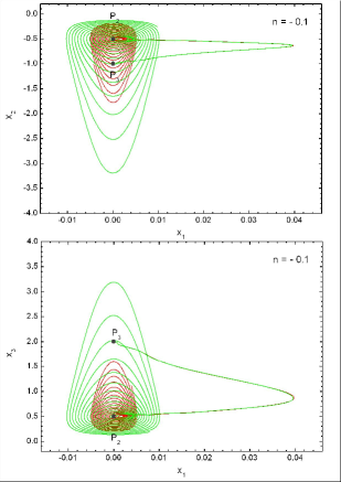
The dynamics of this system has been thoroughly investigated in Amendola (2006), here we just list the main results for the model $f(R)=R+\mu^{2(n+1)}/(-R)^{n}$ for the purpose of completeness. Firstly, it is easy to obtain

$$\left(\frac{\mu^{2}}{-R}\right)^{n+1} = \frac{x_{3}+x_{2}}{x_{3}-nx_{2}}$$ (43)

for the use in the numerical calculation. Secondly, the critical points and their properties of the system are listed in Table 1 where we have defined

$$\Omega_{\mathrm{m}} = \frac{\kappa\rho_{\mathrm{m}}}{3FH^{2}}=1-x_{1}-x_{2}-x_{3}-x_{4},$$ (44)

$$w_{\mathrm{eff}} = -\frac{2\dot{H}}{3H^{2}}-1.$$ (45)

Table 1: The critical points and their properties.

Point	$(x_{1},x_{2},x_{3},x_{4})$	$\Omega_{{}_{m}}$	$\Omega_{\mathrm{rad}}$	$w_{\mathrm{eff}}$
$P_{1}$	$(0,0,0,1)$	0	1	$\frac{1}{3}$
$P_{2}$	$(0,-\frac{1}{2},\frac{1}{2},0)$	1	0	0
$P_{3}$	$(0,-1,2,0)$	0	0	$-1$
$P_{4}$	$(-1,0,0,0)$	2	0	$\frac{1}{3}$
$P_{5}$	$(1,0,0,0)$	0	0	$\frac{1}{3}$
$P_{6}$	$\left(\frac{4(n+1)}{n},\frac{2(n+1)}{n^{2}},\frac{2(n+1)}{n},-\frac{5n^{2}+8n+2}{n^{2}}\right)$	0	$-\frac{5n^{2}+8n+2}{n^{2}}$	$-\frac{3n+4}{3n}$
$P_{7}$	$\left(\frac{3(n+1)}{n},\frac{4n+3}{2n^{2}},\frac{4n+3}{2n},0\right)$	$-\frac{8n^{2}+13n+3}{2n^{2}}$	0	$-\frac{n+1}{n}$
$P_{8}$	$\left(-\frac{2(n+2)}{2n+1},\frac{4n+5}{(2n+1)(n+1)},\frac{n(4n+5)}{(2n+1)(n+1)},0\right)$	0	0	$-\frac{6n^{2}+7n-1}{3(2n+1)(n+1)}$
$P_{9}$	$(-4,5,0,0)$	0	0	$\frac{1}{3}$

It is easy to see from Table 1 that the points $P_{1},P_{2},P_{3}$ correspond to a radiation-dominated era, a matter-dominated era and a de Sitter era, respectively, while $P_{4},P_{5},P_{9}$ cannot lead to any of these three eras and are excluded from further consideration. In Table 2, we summarise the stability and acceleration properties of the critical points other than $P_{4},P_{5},P_{9}$ (limited to the cases in which $-1<n<0$). From this table we see that, for general $-1<n<0,$ we can expect $P_{1},P_{2},P_{3}$ to give a viable cosmology provided that the initial conditions are chosen appropriately. In particular, around $P_{2}$, the evolutionary trajectory of the model is a damped oscillation, and it is finally attracted to the stable de Sitter point $P_{3}$. In Figure 1 we have plotted a phase portrait to illustrate this evolution: we see that evolutions with rather different initial conditions fall towards the vicinity of $P_{2}$ and finally pass it, being attracted to the de Sitter point $P_{3}$ along nearly the same trajectory (with this trajectory itself depending on the value of $n$). Depending on the initial conditions, the region of the oscillation could be very tiny; but the numerical simulation shows that, the oscillation of $x_{1}$ around $0$ is a general result, at least for some period of the evolution.

Figure 2: (Color online) The fractional energy densities $\Omega_{\mathrm{m}}$ (green lines), $\Omega_{\mathrm{rad}}$ (blue lines) and $\Omega_{\mathrm{DE}}\equiv 1-\Omega_{\mathrm{m}}-\Omega_{\mathrm{rad}}$ (red lines) as functions of redshift $z$. We plot the cases for $n=-0.01,-0.1,-0.2$ and $-0.5$ respectively. Note that in general $\Omega_{\mathrm{m0}}>0.3$ because we require $\kappa\rho_{\mathrm{m0}}/3H_{0}^{2}=0.3$ instead and because $F_{0}<1$.

Figure 3: (Color online) The same as FIG. 2, but for the case of $n=0$ ($\Lambda\mathrm{CDM}$).

One can recognise here the connection with our Einstein frame analysis. Note that $\varphi\propto\ln F$, so $\dot{\varphi}\propto\dot{F}/F$ and an oscillation of $x_{1}$ around $0$ corresponds to an oscillation of $\dot{F}$ around $0$, which in turn represents an oscillation of $\dot{\varphi}$ around $0$ (this is just the condition for a $\varphi$ oscillation). Furthermore, the final attraction of the trajectories towards $P_{3}$ is also consistent with our conclusion above, that the universe will finally evolve into a de Sitter stage.

Table 2: The stability and acceleration properties of the critical points ($-1<n<0$).

Point	Eigenvalues	Stability	Acceleration ?
$P_{1}$	$1,4,4,-1$	Saddle	No
$P_{2}$	$-1,\left[3+\frac{3n}{(1+m)^{2}},-\frac{3}{4}\pm\sqrt{-\frac{1}{m}}\right]_{m\rightarrow 0^{+}}$	Saddle	No
$P_{3}$	$-3,-4,-\frac{3}{2}\pm\frac{\sqrt{25+\frac{32}{n}}}{2}$	Stable	Yes
$P_{6}$	$1,4\left(1+\frac{1}{n}\right),\frac{1}{2}+\frac{1}{n}\pm\frac{\sqrt{81n^{2}+132n+36}}{2n}$	Saddle	No
$P_{7}$	$-1,3\left(1+\frac{1}{n}\right),\frac{3(n+1)\pm\sqrt{256n^{4}+864n^{3}+1025n^{2}+498n+81}}{4n(n+1)}$	Stable if $-\frac{3}{4}\leq n\leq\frac{\sqrt{73}-13}{16}$, saddle otherwise	No
$P_{8}$	$-\frac{4n+5}{n+1},-\frac{2(n+2)}{2n+1},-\frac{2(5n^{2}+8n+2)}{(2n+1)(n+1)},-\frac{8n^{2}+13n+3}{(2n+1)(n+1)}$	Stable if $n\geq\frac{\sqrt{73}-13}{16}$, saddle otherwise	$-1<n<-\frac{1}{2}$

Figure 4: (Color online) $F$ as a function of redshift. The red, green, blue and magenta curves are the cases for $n=-0.01,-0.1,-0.2$ and $-0.5$ respectively).

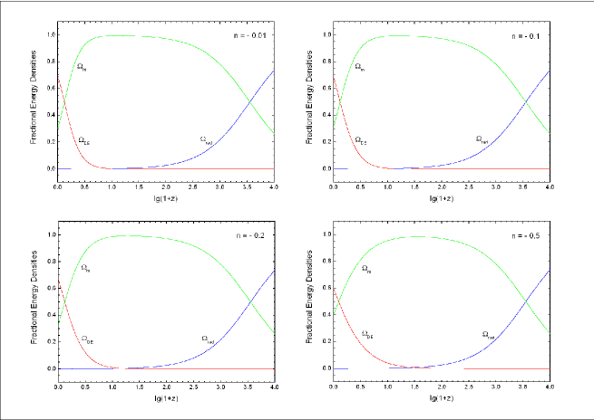
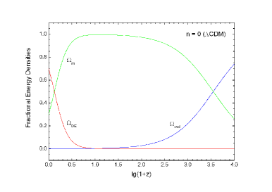
In order to go further, and solve the background equations numerically, we need the detailed initial conditions. One possible way to obtain these is to consider the evolution in the radiation-dominated era. For example, it is possible (in Einstein frame) that the field is frozen in this era Brax (2004) while settling in the vicinity of its effective potential minimum and then starting to oscillate as soon as the fractional matter energy density becomes significant. In our calculation, we use a trial and error method to find the initial conditions at some specified early time which reproduce the observational value $\kappa\rho_{\mathrm{m0}}/3H_{0}^{2}\simeq 0.3$ and $\kappa\rho_{\mathrm{rad0}}/3H_{0}^{2}\simeq 10^{-4},$ where subscript ’0’ denotes the present-day value (note that we are not using $\Omega_{\mathrm{m0}}\simeq 0.3,\Omega_{\mathrm{rad0}}\simeq 10^{-4}$ because of the different definitions Eqs. (36, 44) from conventional cosmology). The results for some specific choices of $n$ are given in Figure 2. Although the difference is not large in the plots, we can see that the $f(R)$ dark energy starts to be significant earlier for larger $|n|$’s. This is as expected because the ratio of correction term in $f(R)$ to $-R$ is given by $[\mu^{2}/(-R)]^{n+1}$ which becomes of order $1$ earlier if $n+1$ is closer to $0$. On the other hand, evolutions of the fractional energy densities are essentially the same as that for $\Lambda\mathrm{CDM}$ at early times when the $f(R)$ corrections are negligible. For reference, we also show the case of $\Lambda\mathrm{CDM}\ (n=0)$ in Figure 3.

Next, we outline the way to obtain all other background quantities from what has already been calculated. Firstly, from Eq. (43) we now have

$$F = (1+n)\frac{x_{3}}{x_{3}-nx_{2}}.$$ (46)

Secondly, from Eq. (36) we get

$$\frac{x_{4}}{x_{40}} = \frac{F_{0}H_{0}^{2}}{FH^{2}}a^{-4},$$

so that

$$H^{2} = \frac{F_{0}x_{40}}{Fx_{4}}a^{-4}H_{0}^{2}.$$ (47)

From Eqs. (33, 35) it follows that

$$\dot{F} = -x_{1}FH,$$ (48)

$$R = -6x_{3}H^{2},$$ (49)

$$\dot{H} = (x_{3}-2)H^{2}.$$ (50)

Finally, Eqs. (25, 26) give

$$\ddot{F} = (1+2x_{1}+3x_{2}+x_{3}-x_{4})FH^{2}.$$ (51)

Consequently, provided $H_{0}$ is known, we can compute any other background quantity.

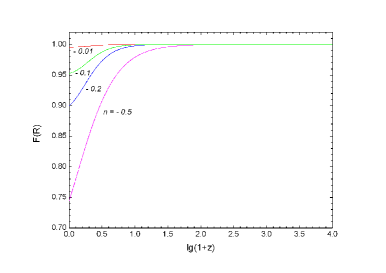
The value of $F$ plays an important role in the $f(R)$ cosmology and so we discuss it separately here. During the matter-dominated era, the trajectory oscillates around the point $P_{2}$, at which $F=1$ exactly. The relation $x_{2}+x_{3}=0$ holds approximately so that $F$ remains close to $1$. At the de Sitter attractor $P_{3}$, we have $x_{2}=-1$ and $x_{3}=2,$ so that $F=(2n+2)/(n+2)$ (corresponding to the potential minimum at $\bar{\varphi}_{0}$ in the Einstein frame). Since our universe has not yet reached $P_{3}$, we expect that $(2n+2)/(n+2)<F_{0}<1$ at present, which is confirmed in Figure 4, where we plot the time evolution of $F$ for the same choices of $n$ as above.

Thus far we have calculated the background quantities $x_{1},x_{2},x_{3},x_{4}$ at some predefined time grid points (scale factor values). Then, in the CAMB code, we can obtain the background quantities at arbitrary times (scale factor values) simply by interpolating between these grid points.

III.3 The CMB and Matter Power Spectra

In the metric $f(R)$ gravity theory, $F$ and $R$ are determined by the energy-momentum tensor $T_{ab}$ through a dynamic equation, as are the perturbations of them, $\hat{\nabla}_{a}F$ or $\hat{\nabla}_{a}R$. To see this, take the covariant spatial derivative of the structural equation and we get

$$\kappa(\hat{\nabla}_{a}\rho-3\hat{\nabla}_{a}p) = 3(\hat{\nabla}_{a}\ddot{F}+\theta\hat{\nabla}_{a}\dot{F}+\dot{F}\hat{\nabla}_{a}\theta+\hat{\nabla}_{a}\hat{\nabla}^{2}F)$$ (52)

$$+R\hat{\nabla}_{a}F-\frac{F}{F_{R}}\hat{\nabla}_{a}F,$$

which should be added to our set of perturbation equations. Since this is a second-order differential equation, we can recast it into two first-order differential equations, which means that we have two more quantities to evolve in the CAMB code, whose initial conditions also need to be specified.

Figure 5: (Color online) The CMB power spectra of the $f(R)$ model. The black, red, green, blue and magenta lines represent the cases of $n=0,-0.01,-0.1,-0.2$ and $-0.5$ respectively. For all the curves we have adopted the parameters $H_{0}=70\ \mathrm{km/s/Mpc}$ and $\kappa\rho_{\mathrm{m0}}/3H_{0}^{2}=0.3$.

Figure 6: (Color online) The potentials $\phi_{k}$ (see definition in text) as functions of the scale factor $a$ for various $k$ values. Only the cases of $\Lambda\mathrm{CDM}\ (n=0)$ (black curves), $n=-0.2$ (red curves) and $n=-0.5$ (green curves) are shown for clearness. The scales are chosen to be $k=0.0005,0.001,0.005,0.01\ \mathrm{Mpc}^{-1}$ as indicated beside the curves. For all the curves we have adopted the parameters $H_{0}=70\ \mathrm{km/s/Mpc}$ and $\kappa\rho_{\mathrm{m0}}=0.3$.

Making a harmonic expansion of $\hat{\nabla}_{a}F$ as

$$\hat{\nabla}_{a}F=\sum_{k}\frac{k\epsilon}{a}Q_{a}^{k},$$

where $Q_{a}^{k}=\frac{a}{k}\hat{\nabla}_{a}Q^{k}$ and $Q^{k}$ are the zero-order eigenvalues of the comoving Laplacian $a^{2}\hat{\nabla}^{2}$ so that $a^{2}\hat{\nabla}^{2}Q^{k}=k^{2}Q^{k}$ Lewis (2000), it is easy to show that

$$\hat{\nabla}_{a}\dot{F} = \sum_{k}\frac{k\dot{\epsilon}}{a}Q_{a}^{k},$$ (53)

$$\hat{\nabla}_{a}\ddot{F} = \sum_{k}\frac{k\ddot{\epsilon}}{a}Q_{a}^{k},$$ (54)

with the aid of

$$\hat{\nabla}_{a}\dot{\psi}\doteq(\hat{\nabla}_{a}\psi)^{\cdot}+\frac{1}{3}\theta\hat{\nabla}_{a}\psi$$

for any scalar $\psi$ (the $\doteq$ means that we obtain this relation in the frame where the acceleration $A_{a}=0$, see Lewis (2000)). At early times, when $F=1,\dot{F}=0$, Eq. (52) reduces to

$$\frac{\kappa(\mathcal{X}-3\mathcal{X}^{p})}{3H^{2}}$$ (55)

$$\approx \epsilon^{\star\star}+\frac{3}{2}\epsilon^{\star}+\left[\frac{R}{3H^{2}}\left(1-\frac{1}{RF_{R}}\right)+\frac{k^{2}}{a^{2}H^{2}}\right]\epsilon,$$

in which $\mathcal{X},\mathcal{X}^{p}$ are defined through the harmonic expansions $\hat{\nabla}_{a}\rho=\sum_{k}k\mathcal{X}Q_{a}^{k}/a$ and $\hat{\nabla}_{a}p=\sum_{k}k\mathcal{X}^{p}Q_{a}^{k}/a$, and a star denotes the derivative with respect to $\ln a$. Recall that in the matter-dominated era $|R/H^{2}|\sim 1$, $\kappa(\mathcal{X}-3\mathcal{X}^{p})/3H^{2}=\kappa\rho_{\mathrm{m}}\Delta_{\mathrm{m}}/3H^{2}\sim\Delta_{\mathrm{m}}$, where $\Delta_{\mathcal{\mathrm{m}}}$ is the fractional perturbation in non-relativistic matter components (the contribution from photons and massless neutrinos to this term is zero because $\mathcal{X}_{\gamma,\nu}^{p}=\mathcal{X}_{\gamma,\nu}/3$) and

$$1-\frac{1}{RF_{R}}=1+\frac{1}{n(n+1)\left(\frac{\mu^{2}}{-R}\right)^{n+1}}$$

tends to $-\infty$ (for $-1<n<0$) as $\mu^{2}/(-R)\rightarrow 0$. So, early in the matter-dominated era, the coefficient in front of $\epsilon$ becomes very large (remember again that $R<0$) and $\epsilon$ settles to $\sim\Delta_{\mathrm{m}}/|1-1/RF_{R}|$ within a short time Song (2006). This means that the actual result will be insensitive to the choice of initial conditions, a fact we have checked using the numerical code. Thus, for our calculation, we can simply set $\epsilon_{\mathrm{initial}}=\dot{\epsilon}_{\mathrm{initial}}=0$. In this model, the perturbation in $F$ is driven essentially to zero (compared with the matter perturbation) and finally grows as dark energy starts to drive the expansion of the universe. It is also interesting to note that according to the analysis above, when $n=0^{-}$ we have $F_{R}=0^{-}$ and so the perturbation, $\epsilon$, will stay zero all through cosmic history, which is consistent with the property of an effective cosmological constant.

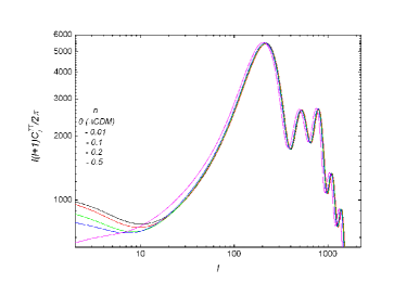
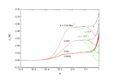
In Figure 5, we plot the CMB power spectrum of the model for different choices of $n$. For all of these plots we again adopt $H_{0}=70\ \mathrm{km/s/Mpc}$ and $\kappa\rho_{\mathrm{m0}}/3H_{0}^{2}=0.3$. Two effects can immediately be seen to occur in the spectrum. Firstly, the locations of the acoustic peaks move towards the lower $l$s as $|n|$ increases. This is because, for larger $|n|,$ the dark-energy term starts to be important earlier and, with $H_{0}$ fixed, the universe has a smaller age today, which causes the peaks to shift leftwards. This effect is not very significant when $n$ is small. Secondly, we see a reduction of power at low $l$s, which was also been found and discussed in Song (2006), although there the background expansion is fixed to match the $\Lambda\mathrm{CDM}$ cosmology. This reduction in low-$l$ power is caused by a weaker late-time decay of the large-scale potential $\phi_{k}$ (which is the coefficient of the harmonic expansion of $\mathcal{E}_{ab}$ as $\mathcal{E}_{ab}=-\sum_{k}k^{2}\phi_{k}Q_{ab}^{k}/a^{2}$ and related to the Newtonian potential $\Psi$ by $\Psi=\phi-\kappa\Pi a^{2}/2k^{2}$ for any specified $k$-mode where $\Pi$ is the anisotropic stress Lewis (2000)) compared with that in $\Lambda\mathrm{CDM}$, that leads to a suppression on the Integrated Sachs-Wolfe (ISW) effect and thus of the $C_{l}$ at low $l$s. In Figure 6 we give some plots for the evolution of the potential at different scales ($k$’s) in this model, which clearly show the slower decay at large scales Comment (2006). Note that this is remarkably different from the cases of Palatini $f(R)$ gravities, in which the potentials decay much more rapidly than that in $\Lambda\mathrm{CDM}$ Li (2006, 2006), leading to significant amplifications of the low-$l$ power. Also, we see that this model is potentially useful in reducing the difference between the predicted and measured CMB powers at low $l$.

Figure 7: (Color online) The matter power spectra of the $f(R)$ model. The black, red, green, blue and magenta lines represent the cases of $n=0,-0.01,-0.1,-0.2$ and $-0.5$ respectively. In all these plots we have adopted $H_{0}=70\ \mathrm{km/s/Mpc}$ and $\kappa\rho_{\mathrm{m0}}/3H_{0}^{2}=0.3$.

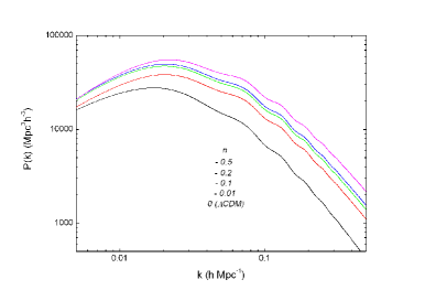
The linear matter power spectra at $z=0$ of the present models are shown in Figure 7. From this plot we can see that the matter power spectrum has similar behavior to those in the case of a general $f(R)$ model with $\Lambda\mathrm{CDM}$ background evolution Song (2006). On small scales the spectra arising in the $f(R)$ gravity theories we are considering have similar shapes to the case of the $\Lambda\mathrm{CDM}$ power spectrum, and this fact can be understood roughly, as follows. Consider for simplicity the growth of the dark-matter fractional density perturbation $\Delta_{\mathrm{c}},$ which is defined by $\rho_{\mathrm{c}}\Delta_{\mathrm{c}}=\mathcal{X}_{c}$ (essentially the $\delta_{\mathrm{c}}$ in CMBFAST), in a universe filled with cold dark matter and photons. After some manipulations of our set of perturbation equations it is easy to show that in metric $f(R)$ theories:

$$\Delta_{\mathrm{c}}^{\prime\prime}+\left(\mathcal{H}-\frac{F^{\prime}}{F}\right)\Delta_{\mathrm{c}}^{\prime}$$ (56)

$$= \frac{1}{F}\kappa\mathcal{X}a^{2}-\frac{1}{F}k^{2}\epsilon-\frac{3}{F}\mathcal{H}\epsilon^{\prime}-\frac{3}{2F}\frac{\mathcal{H}^{\prime\prime}+\frac{F^{\prime}}{F}\mathcal{H}^{\prime}}{\mathcal{H}+\frac{F^{\prime}}{2F}}\epsilon$$

$$+\frac{\frac{3\mathcal{H}}{F}(\mathcal{H}^{\prime}+\mathcal{H}^{2})\left(1-\frac{F}{RF_{R}}\right)}{\mathcal{H}+\frac{F^{\prime}}{2F}}\epsilon$$

where a prime represents the derivative with the conformal time $\tau$ ($ad\tau=dt$) and $\mathcal{H}=a^{\prime}/a$. At the same time, Eq. (52) can now be rewritten as

$$\kappa(\mathcal{X}-3\mathcal{X}^{p})a^{2} = 3(\epsilon^{\prime\prime}+2\mathcal{H}\epsilon^{\prime}+kF^{\prime}\mathcal{Z}+k^{2}\epsilon)$$ (57)

$$-6(\mathcal{H}^{\prime}+\mathcal{H}^{2})\left(1-\frac{F}{RF_{R}}\right)\epsilon$$

where $\mathcal{Z}$ is the harmonic expansion coefficient of $\hat{\nabla}_{a}\theta$ ($\hat{\nabla}_{a}\theta=\sum_{k}k^{2}\mathcal{Z}Q_{a}^{k}/a^{2}$). In the CDM frame (in which $v_{c}=0$) we have Lewis (2000)

$$\Delta_{\mathrm{c}}^{\prime} = -k\mathcal{Z}.$$ (58)

A similar analysis to that below Eq. (55) then shows that, for small scales which are characterised by $k^{2}/\mathcal{H}^{2}\gg 1$, the term $3k^{2}\epsilon$ dominates the right-hand side of Eq. (57) provided that $|F_{R}|$ is not too close to $0$, which is the case for the later stages in our $f(R)$ cosmology. Thus, we have now

$$\kappa(\mathcal{X}-3\mathcal{X}^{p})a^{2} \approx 3(kF^{\prime}\mathcal{Z}+k^{2}\epsilon),$$ (59)

which we have also verified numerically.

Substituting Eqs. (58, 59) into Eq. (56), we get (neglecting the contribution from relativistic energy components):

$$\Delta_{\mathrm{c}}^{\prime\prime}+\mathcal{H}\Delta_{\mathrm{c}}^{\prime}-\frac{2}{3F}\kappa\rho_{\mathrm{c}}\Delta_{\mathrm{c}}a^{2} \approx 0.$$ (60)

Interestingly, we have obtained a scale-independent behavior for the CDM density perturbation growth on small scales, similar to that of standard GR, where it is given by

$$\Delta_{\mathrm{c}}^{\prime\prime}+\mathcal{H}\Delta_{\mathrm{c}}^{\prime}-\frac{1}{2}\kappa\rho_{\mathrm{c}}\Delta_{\mathrm{c}}a^{2} \approx 0.$$ (61)

This explains why on small scales the shape of the $f(R)$ matter power spectrum is like that of $\Lambda\mathrm{CDM}$ (see Koivisto (2006) for a similar example). It also indicates that the growths of small-scale perturbations are governed by an effective gravitational constant given by $\kappa_{\mathrm{eff}}=4\kappa/3F>\kappa$. Notice that one should not simply try to put $F=1$ into Eq. (60) to get the $\Lambda\mathrm{CDM}$ limit, since under this condition the last term in Eq. (57) always dominates over $3k^{2}\epsilon$ and can never be neglected. The correct $\Lambda\mathrm{CDM}$ limit is recovered by setting $F^{\prime}=0,F=1,6(\mathcal{H}^{\prime}+\mathcal{H}^{2})(1-F/RF_{R})\epsilon=-\kappa(\mathcal{X}-3\mathcal{X}^{p})a^{2},$ (according to Eq. (57)) and all other terms relating $\epsilon$ and $\epsilon^{\prime}$ to $0$ in Eq. (56), which just leads to Eq. (61), and shows that the early-matter-era growth of perturbations is well described by GR.

Figure 8: (Color online) The dependence of the matter power spectra on $H_{0}$ (upper panel) and $\kappa\rho_{\mathrm{m0}}/3H_{0}^{2}$ (lower panel). Upper panel: the black, red, green solid curves represent $H_{0}=65,68,70\ \mathrm{km/s/Mpc}$ respectively ($\kappa\rho_{\mathrm{m0}}/3H_{0}^{2}=0.3$). Lower panel: the black, red, green curves represent $\kappa\rho_{\mathrm{m0}}/3H_{0}^{2}=0.25,0.27,0.30$ respectively ($H_{0}=70\ \mathrm{km/s/Mpc}$). Dashed curves are the spectra for the $\Lambda\mathrm{CDM}$ model. $n=-0.5$ is adopted for illustration. We see that a smaller $\kappa\rho_{\mathrm{m0}}/3H_{0}^{2}$ can bring the shape of the spectrum closer to the $\Lambda\mathrm{CDM}$ one: in this case data on large scale structure cannot place stringent constraints on the model.

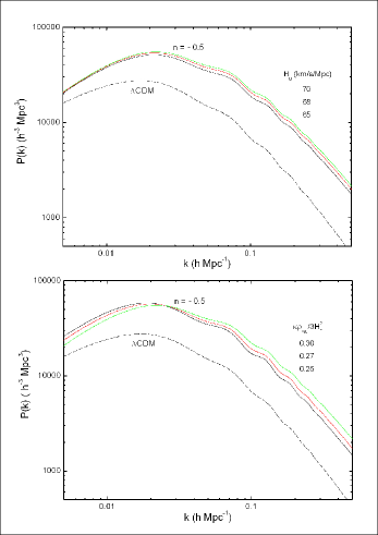
We can now make a comparison between the matter power spectra in metric and Palatini $f(R)$ cosmologies. In the later, it has been shown that any small deviation from GR will cause the small-scale spectra to differ from the GR one in observationally unacceptable ways, either blowing up or oscillating and being prevented from growing Koivisto (2006); Li (2006, 2006). This is because in the Palatini $f(R)$ gravity $F$ and $T$ satisfy an algebraic equation $F=F(T)$ such that those terms involving $\hat{\nabla}^{2}F$ can always be rewritten as $\propto\hat{\nabla}^{2}T\sim\hat{\nabla}^{2}\rho$ and consequently a term $\propto k^{2}\Delta_{\mathrm{c}}$ appears in the growth equation which makes the growths on small scales strongly scale-dependent. In the metric $f(R)$ gravity here, in contrast, $\epsilon$ is determined by the perturbations in $T$ through a differential equation Eq. (57). As $k$ increases, the value of the perturbation in $F(\epsilon)$ decreases, so that $k^{2}\epsilon$ does not exceed $\mathcal{O}(\kappa\mathcal{X}a^{2})$ and becomes $k$ independent, so its effect cannot be as exotic as that arising in Palatini $f(R)$ theories.

Before leaving this analysis, we want to briefly discuss the cosmological viability of the present model. A more rigorous analysis involves carefully searching the multidimensional parameter space (as in Li (2006)) and is beyond the scope of the present work. Firstly, we have seen that the background evolutions allowed by the model are rather close to the $\Lambda\mathrm{CDM}$ paradigm with particular choices of $n,$ and so could be consistent with the SNIa observations. The confrontation between predictions and the data on the linear power spectrum is a little more complicated. For the CMB spectrum, Figure 5 indicates that it is similar to the $\Lambda\mathrm{CDM}$ prediction at higher $l$’s and can also reduce the quadrupole power and bring it closer to the measured values Song (2006) (We have also checked that this low-$l$ power reduction is a general feature of the model and is insensitive to the values of $H_{0}$ and $\rho_{\mathrm{m}0}$). However, because of the limitation from cosmic variance, the influences on the likelihood analysis are expected to be small. For the matter spectrum, at small scales the power is significantly higher than for the $\Lambda\mathrm{CDM}$ case, yet the fact that it has similar shape to the latter indicates the possibility that a different choice of galaxy bias might be able to make the model’s predictions consistent with, for example, the Sloan Digital Sky Survey (SDSS) observations. However, we notice that at wavenumber $k\sim 0.05\ h\mathrm{Mpc^{-1}}$ deviations from the $\Lambda\mathrm{CDM}$ shape start to be significant, which might potentially be in conflict with the data; this could still be alleviated by reducing the quantity $\kappa\rho_{\mathrm{m0}}/3H_{0}^{2}$, as can be seen in Figure 8.

We conclude that constraints on this model from large-scale structure could be much weaker than those on the Palatini $f(R)$ models Li (2006, 2006). This said, it is still interesting to obtain quantitative joint constraints from background cosmology, CMB, and matter power spectra on the model, and examine whether it can be made consistent with other cosmological observations (such as considered in Song (2006)) in the future.

IV Discussion and Conclusions

To summarise: in this article we have considered the cosmology of a subclass of metric $f(R)$ gravity theories, that are characterised by $f(R)=R+\mu^{2(n+1)}/(-R)^{n}$, and have discussed both the flat background Friedmann universe and its inhomogeneous perturbations. For the background evolution, we address the problem in both the Jordan frame and the Einstein frame and find the correspondences between them. Generally, the evolution is attracted towards a saddle point in the phase space which has the characteristics of a matter-dominated era. If the initial conditions are chosen appropriately, the universe can stay in the vicinity of that point for a sufficiently long period of CDM-dominated evolution to occur. Finally, it always passes this saddle point and evolves to a stable de Sitter point. The cosmic expansion begins to accelerate during this transition period and a cosmic history that is consistent with observations is possible in this model, as expected from Amendola (2006). In the Einstein frame, the model reduces to one with a scalar field conformally coupled to (non-relativistic) matter, and it shares some of the properties of a chameleon field cosmologies. That cosmological model results in a matter-dominated era followed by an accelerating era can also be seen from the analysis in this frame. The $\Lambda\mathrm{CDM}$ limit of the model is also discussed.

We derive the covariant and gauge invariant perturbation equations for $f(R)$ gravity theories in general, which we believe to be rather convenient for numerical calculations, and applied them to the present model through a modified CAMB code. The linear spectra are obtained and discussed. The CMB power spectrum displays reductions in the low-$l$ power, which arises from a weakening of the ISW effect because of insufficient late-time decay of the large-scale potentials, as shown in the plots of the evolution. For the matter power spectrum, we find that on small scales the matter density growth is nearly scale-independent, making the shape of the spectrum at large $k$’s similar to that of the $\Lambda\mathrm{CDM}$ spectrum. Comparisons with the CMB and matter power spectra in Palatini $f(R)$ gravity theories are then made, which account for the dramatic differences between these two approaches to modify GR, despite the fact that they could have the same gravitational action.

Possible comparisons with different observational data sets are also briefly discussed. It is found that neither the data on background evolution, CMB spectrum, nor those on the matter power spectrum can be used to exclude the model. Their joint constraints on the model, however, could be complicated and involve making a numerical search of the parameter space, which is beyond the scope of the present work. However, we can see that constraints on this metric $f(R)$ model could be much weaker than those on the Palatini $f(R)$ theories, because for the later (1) the CMB power is largely amplified at low $l$’s and (2) the matter power spectrum at small scales is strongly scale dependent, both conflicting with observations on CMB anisotropies and large scale structure.

The form of $f(R)$ adopted here is one of the few which could produce a viable model for the entire cosmic history. In this model the modifications to GR take effect only at late times. Therefore, it is interesting to look for other models in which the modifications are significant at different times, along the lines of refs. Li (2006); Bean (2006). In Li (2006), a model with $f(R)=R+\lambda_{1}\exp(R/\lambda_{2})$ is considered in the Palatini approach and its effects on the linear power spectra are also discussed. In Bean (2006), this same model is investigated within the metric approach; however, it actually gives a $\phi$-matter-dominated era ($\phi\mathrm{MDE}$), Amendola (2006, 2000), rather than the standard matter-dominated era, and is not cosmologically viable. Thus, it may still be meaningful to look for viable early-time $f(R)$ cosmologies in the metric formalism. Another interesting issue to explore is whether the $f(R)$ gravity models might be more adapted to hot dark matter. These topics will be investigated elsewhere.

Notes Added: there is recently another paper Faulkner (2006) discussing the Chameleon properties of the $f(R)$ theories, but the emphasis is different from ours here. See also Navarro (2006).