Mining information from binary black hole mergers:
a comparison of estimation methods for complex exponentials in noise

Abstract

The ringdown phase following a binary black hole merger is usually assumed to be well described by a linear superposition of complex exponentials (quasinormal modes). In the strong-field conditions typical of a binary black hole merger, non-linear effects may produce mode coupling. Artificial mode coupling can also be induced by the black hole’s rotation, if the radiation field is expanded in terms of spin-weighted spherical harmonics (rather than spin-weighted spheroidal harmonics). Observing deviations from the predictions of linear black hole perturbation theory requires optimal fitting techniques to extract ringdown parameters from numerical waveforms, which are inevitably affected by numerical error. So far, non-linear least-squares fitting methods have been used as the standard workhorse to extract frequencies from ringdown waveforms. These methods are known not to be optimal for estimating parameters of complex exponentials. Furthermore, different fitting methods have different performance in the presence of noise. The main purpose of this paper is to introduce the gravitational wave community to modern variations of a linear parameter estimation technique first devised in 1795 by Prony: the Kumaresan-Tufts and matrix pencil methods. Using “test” damped sinusoidal signals in Gaussian white noise we illustrate the advantages of these methods, showing that they have variance and bias at least comparable to standard non-linear least-squares techniques. Then we compare the performance of different methods on unequal-mass binary black hole merger waveforms. The methods we discuss should be useful both theoretically (to monitor errors and search for non-linearities in numerical relativity simulations) and experimentally (for parameter estimation from ringdown signals after a gravitational wave detection).

I Introduction

The last year witnessed a remarkable breakthrough in numerical relativity. Many different groups were finally able to evolve black hole binaries through the last few cycles of inspiral, merger and ringdown and to extract gravitational waveforms from the evolutions Bruegmann:2003aw ; Pretorius:2005gq ; Campanelli2006 ; Baker2006 ; Herrmann:2006ks ; Sperhake:2006cy ; Scheel:2006gg ; Bruegmann:2006at ; Gonzalez:2006md ; Szilagyi:2006qy . If numerical simulations start out at large enough separation, it should be possible to match them with Post-Newtonian predictions for the inspiral signal. This is a very active research area Berti:2006bj ; Buonanno:2006ui ; Baker:2006ha . Studies of equal-mass merger simulations starting from different orbital separations (or produced by different numerical techniques) show that, independently of the waveform accuracy in the pre-merger phase, the strong-field waveform has a “universal” shape. Preliminary, “first order” explorations of the merger waveform for equal-mass black hole binaries indicate that the merger phase is short-lived, lasting only $\sim 0.5-0.75$ gravitational wave (GW) cycles Buonanno:2006ui . After this short merger the signal has the typical “ringdown” shape – i.e., it is well modelled by a superposition of complex exponentials, known as quasinormal modes (QNMs).

QNMs play a role in any astrophysical process involving stars and black holes. Oscillations of a relativistic star and of a black hole necessarily produce GWs KokkotasSchutz ; vish ; Leaver:1985ax . In linear perturbation theory the metric perturbations can usually be described by a single scalar function, which, in the ringdown phase, can be written as a superposition of complex exponentials:

$$\Psi_{lm}(t)=\sum_{n}A_{lmn}e^{(\alpha_{lmn}+i\omega_{lmn})t+i\varphi_{lmn}}\,.$$ (1)

Here $A_{lmn}$, $\varphi_{lmn}$, $\omega_{lmn}$ and $\tau_{lmn}=-\alpha_{lmn}^{-1}$ are the mode’s amplitude, phase, frequency and damping time respectively. The indices $(l\,,m)$ describe the angular dependence of the signal, and the index $n$ sorts the modes by the magnitude of their damping time. The amplitude and phase is determined by the specific process exciting the oscillations. Remarkably, in linear perturbation theory the QNM frequencies $\omega_{lmn}$ and damping times $\tau_{lmn}$ are uniquely determined by the mass and angular momentum of the black hole: this is a consequence of the so-called “no hair” theorem of general relativity. For this reason, accurate QNM measurements could provide the “smoking gun” for black holes and an important test of general relativity in the strong-field regime (see eg. bcw , listing the dominant QNM frequencies for rotating black holes and providing fits of the numerical results).

In the GW literature it is often claimed that “the ringdown phase is well described by (linear) black hole perturbation theory, and that the ringdown waveform is given by a simple superposition of damped exponentials” of the form (1). This statement is based on two tacit assumptions, that may well be false under the strong-field conditions typical of a binary black hole merger:

• Non-linearities are negligible, so that linear perturbation theory applies. However, non-linear effects should be present in binary black hole merger waveforms. Model problems show that non-linearities are responsible for a systematic shift in the quasinormal frequencies and, more interestingly, for mode coupling Zlochower:2003yh .

• Mode coupling is negligible. Even if assumption (i) above is valid and non-linear effects are small, different multipolar components can still be coupled. For example, artificial mode coupling can arise because of some commonly used approximations in the wave extraction process.

An important open problem in the interpretation of merger waveforms is to isolate general relativistic non-linearities from artificial effects induced by unwanted features of the numerical simulations, such as finite-differencing errors, errors due to the approximate nature of initial data or spurious rotational QNM coupling induced by the use of spin-weighted spherical harmonics in GW extraction. All of these effects depend on the details of the numerical implementation and of the wave extraction procedure. The ultimate goal of GW detection is to assess the validity of general relativity in the strong-field regime, so the relevance of this problem can hardly be underestimated. Understanding non-linear phenomena unique to general relativity is of paramount importance if we want to discriminate Einstein’s theory from alternative theories of gravity, that may give different predictions in strong-field situations. Since most of the strong-field waveform can be described as a QNM superposition, strong-field effects could well show up in the fine structure of this QNM superposition: in particular, non-linearities may manifest themselves as time variations of the ringdown frequencies, or as beating phenomena between different QNMs.

In this paper we take a first step towards the solution of this problem. We consider intrinsic limitations of the fitting routines used to extract quasinormal ringing parameters, exploring the properties of different fitting techniques for the extraction of ringdown parameters from numerical waveforms. This issue can be studied independently of the details of any given merger simulation. The idea is that, by quantifying the limitations of a given fitting method, we should be able to isolate systematic uncertainties (due to the fact that we are fitting noisy numerical waveforms) from possibly more interesting physical features of the waveforms themselves.

The problem of estimating the parameters of complex exponentials in noise has a long history in science and engineering. Damped sinusoidal signals are the “real-world counterpart” of the harmonic oscillators used in Fourier analysis. Therefore, estimating the parameters of damped sinusoids is of primary importance in physics. Examples include (i) speech and audio modelling audiom , (ii) angle-of-arrival estimation of plane waves impinging on sensor arrays for radar purposes or radio-astronomy, and antennae array processing antennae , (iii) estimation of lifetimes and intensities in radioactive decay positronlifetime , (iv) nuclear magnetic resonance and computer assisted medical diagnosis djermoune . This list can be extended to include spectroscopy, the study of mechanical vibrations (including seismic signal processing), the diffusion of chemical compounds, economics, and so on.

Fits of ringdown waveforms are usually performed using standard non-linear least-squares methods (see eg. Dorband:2006gg ; Buonanno:2006ui and references therein). These methods are known to fail in estimating parameters for a sum of damped exponentials. In this case, minimizing the squared error over the data requires the solution of highly non-linear expressions in terms of sums of powers of the damping coefficient. No analytic solution is available, and these expressions can usually be solved only with a good initial guess for the parameters marplebook . Even for a single damped exponential, if the initial guess is inaccurate the algorithm often fails to converge. Iterative algorithms, such as gradient descent procedures or Newton’s method, have been devised to minimize these non-linear expressions. Unfortunately the algorithms are computationally very expensive, sometimes requiring at each step the inversion of matrices of dimension as large as the number of data samples iterative . Furthermore, gradient descent algorithms for multimodal equations sometimes fail to converge to the global minimum.

Computational difficulties with non-linear least-squares methods led to the development of suboptimal estimation methods based on linear prediction equations marplebook ; djermoune . These methods are modern variations on a 1795 paper by Gaspard Riche, Baron de Prony prony , who introduced a procedure to exactly fit $N$ data points by as many purely damped exponentials as needed. Modern versions of Prony’s method generalize the original idea to damped sinusoidal models. They also make use of least-squares analysis to approximately fit an exponential model for cases where the data points cannot be fitted by the assumed number of exponential terms. Unfortunately, these “modified least-squares Prony methods” are very sensitive to numerical noise. Two successful improvements of these methods, the Kumaresan-Tufts (KT) kumaresantufts and matrix pencil (MP) matrixpencil techniques, make use of singular value decomposition to improve parameter estimation accuracy in the presence of noise. For excellent reviews of these and other estimation methods we refer the reader to the first chapter of djermoune (in French) and to Marple’s book marplebook . A purpose of this paper is to introduce these estimation methods to the GW community.

The plan of the paper is as follows. To put our problem in perspective, in Section II we describe the main features of our numerical simulations of binary black hole mergers and of the resulting waveforms. In Section III we summarize the theory behind different estimation methods, and in Section IV we list the numerical algorithms we implemented in our comparisons. In Section V we compare the performance of linear estimation methods (MP and KT) against non-linear least squares methods, by performing Monte Carlo simulations of damped sinusoidal signals in Gaussian white noise. In Section VI, we apply different fitting methods to selected waveforms generated by numerical relativity simulations. Finally we summarize our results and indicate possible directions for further research.

II Numerical simulations

In this Section we briefly describe the numerical simulations of non-spinning, unequal-mass black hole binaries previously presented in Gonzalez:2006md . The simulations were performed with the Bam code Bruegmann:2006at , using the so-called “moving puncture” method. This method, originally introduced in Refs. Campanelli2006 ; Baker2006 , is now being used almost routinely by various groups to successfully perform numerical simulations of inspiralling and merging black hole binaries. Our simulations of the inspiral of unequal-mass black hole binaries are the same used to study recoil in Ref. Gonzalez:2006md . Details of these simulations, of the numerical setup and of the Bam code are given in Refs. Bruegmann:2006at ; Gonzalez:2006md . The main purpose of this paper is to test fitting methods to extract QNMs from the simulations. Therefore we defer a detailed investigation of the unequal-mass waveforms and of their physical properties to a forthcoming publication follow-ups .

In the absence of spin, a standard conformally flat black hole binary initial data set is uniquely determined by the parameters $m_{1}$, $m_{2}$, $\vec{P}_{1}$, $\vec{P}_{2}$, $D$ which denote, in this order, the bare masses and linear momenta of the individual holes, and their coordinate separation. The specification of these parameters allows us to compute the total Arnowitt-Deser-Misner (ADM) mass $M$ of the system, the orbital angular momentum $L=(P_{1}+P_{2})D$, the individual black hole masses $M_{1}$, $M_{2}$ and the mass ratio $q=M_{1}/M_{2}$. Finally, the sum of the individual holes’ spins and of the orbital angular momentum gives the total ADM angular momentum $J$ of the system.

In the parameter study under consideration, the mass ratio $q$ was varied while keeping constant the initial coordinate separation $D=7\,M$ of the black holes. The linear momenta of the individual holes then follow from the requirement that the system represent a quasi-circular configuration. For a given separation $D$, the momentum of each puncture can thus be calculated to third-order post-Newtonian accuracy in the Arnowitt-Deser-Misner, transverse-traceless (ADMTT) gauge. The resulting relation is given by Eq. (64) in Bruegmann:2006at and forms the basis for all initial data sets discussed in this work. The parameters used in our simulations are summarized in Table 1.

Table 1: Total ADM mass, angular momentum and initial binding energy of the unequal mass binaries.

$q$	$M$	$J/M^{2}$	$-E_{\rm b}/M$
1.00	0.9935	0.8845	0.0140
1.49	1.2422	0.8494	0.0134
1.99	1.4914	0.7870	0.0124
2.48	1.7408	0.7232	0.0114
2.97	1.9904	0.6649	0.0104
3.46	2.2401	0.6132	0.0096
3.95	2.4899	0.5679	0.0089

In the notation of Ref. Bruegmann:2006at , the simulations have been performed using the $\chi_{\eta=2}$ approach of the moving puncture method with a number of grid points $i=56,~{}64,~{}72$ on the three innermost refinement levels, respectively. This corresponds to resolutions of $h=1/45$, $1/51$ and $1/58$. In this work we use the waveforms resulting from the low-resolution and high-resolution simulations, using $i=56$ and $i=72$ grid points, respectively. The wave extraction procedure is based on the Newman-Penrose formalism. The Weyl scalar $\Psi_{4}$ is extracted according to the method described in Sec. III A of Bruegmann:2006at . In all simulations presented in this work, $\Psi_{4}$ is calculated at extraction radius $r_{\rm ex}=30M$. Further details of the numerical setup are given in Ref. Gonzalez:2006md .

Figure 1: Real and imaginary parts of $rM\psi_{lm}$ for the two dominant multipoles. The binary has mass ratio $q=1.5$. The burst of radiation at early times is induced by the initial data. After the initial burst, the real and imaginary parts are simply related by a phase shift (i.e., the waveform is circularly polarized). The irregular behavior at late times is due to numerical noise.

Figure 2: $|rM\psi_{lm}|$ for different multipoles. The high-resolution $l=m=2$, $l=m=3$ and $l=m=4$ wave amplitudes have maxima at $t_{\rm peak}/M=236.4,~{}238.4$ and $~{}235.7$, respectively. Wiggles at late times are due to numerical noise, mainly caused by reflections from the boundaries.

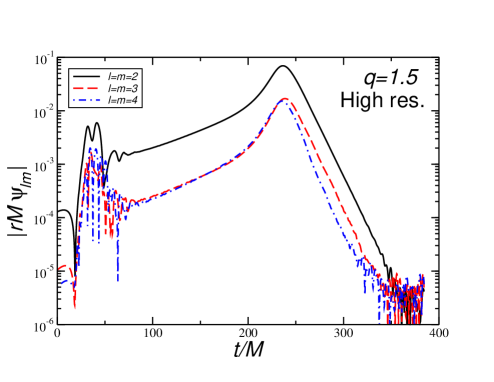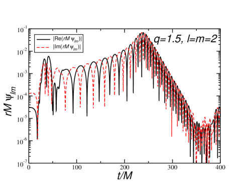
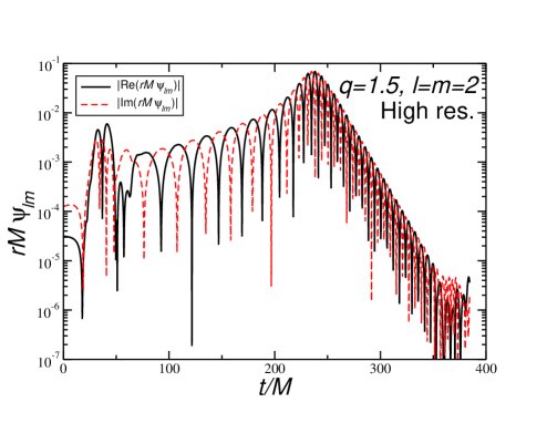
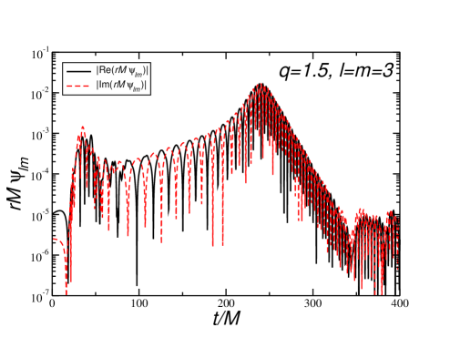
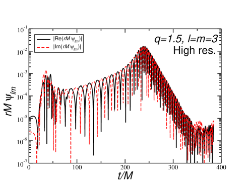
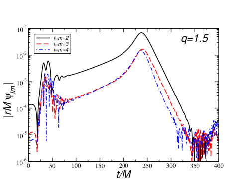
To illustrate some issues related with the extraction of ringdown information from numerical waveforms, in Fig. 1 and Fig. 2 we show the complex mode amplitudes $rM\psi_{lm}$ and their modulus $|rM\psi_{lm}|$ for the dominant components of the radiation emitted by a binary with mass ratio $q=1.5$. Because of the reflection symmetry of the system (see Bruegmann:2006at ), real and imaginary parts of the positive-$m$ and negative-$m$ components are related by

$$\psi_{l-m}=(-1)^{l}(\psi_{lm})^{*}\,.$$ (2)

Components with $|m|<l$ or $l>4$ usually contain significant numerical noise, and we will ignore them in the following.

At early times the waveform is contaminated by a spurious burst of radiation, due to the approximate nature of the initial data. After this initial data burst, the frequency and amplitude of the wave grow as the binary members come closer, producing the characteristic “chirping” gravitational waveform. Eventually the binary members merge, the wave amplitude reaches a maximum, and then it decays as the remnant black hole settles down to a stationary Kerr state, emitting ringdown waves. The final part of the ringdown waveform is visibly contaminated by some amount of numerical noise, that decreases as we increase the resolution. This noise is mainly due to radiation being reflected from the boundaries of the computational domain.

The plots clearly show that the real and imaginary parts of the waveform follow the same pattern, except for a (roughly) constant phase shift. This means that the waveform is circularly polarized Baker:2002qf . From the point of view of extracting information from the ringdown, circular polarization means that fitting the real or the imaginary part should make no difference: to a good approximation, we should get the same results for the oscillation frequencies and damping times. Fitting methods capable of directly dealing with complex waveforms (such as the Prony-type methods considered in this paper) should be particularly useful for waveforms with general polarization, such as those that should be emitted by the generic merger of spinning, precessing black holes.

Independently of the chosen fitting method, there is some arbitrariness in the choice of the time window $[t_{0},~{}t_{f}]$ used to perform the fit. A well-known problem with the transition merger-ringdown is that we do not know a priori when the ringdown starts (see Buonanno:2006ui ; Berti:2006wq ; Dorband:2006gg and references therein). Ideally, the starting time $t_{0}$ should be determined by a compromise between the following requirements: (i) $t_{0}$ should be small enough to include the largest possible number of data points: in particular, we do not want to miss the large amplitude, strong-field part of the waveform right after the merger; (ii) $t_{0}$ should be large enough that we do not include parts of the waveform which are not well described by a superposition of complex exponentials: the inclusion of inspiral and merger in the ringdown waveform would produce a bias in the QNM frequencies.

A judicious choice of $t_{f}$ is also necessary. Usually we would like the time window to be as large as possible, but a glance at Fig. 1 and Fig. 2 shows that the low amplitude, late-time signal is usually dominated by numerical noise, mainly caused by reflections from the boundaries. This noise can reduce the quality of the fit, especially for the subdominant components with $l>2$ and for large values of $t_{0}$. A practical criterion for the choice of $t_{f}$ is suggested by a look at Fig. 2. If the ringdown waveform were not affected by noise from boundary reflections, $|rM\psi_{lm}|$ should decay linearly on the logarithmic scale of the plots. At low signal amplitudes, we see boundary noise-induced wiggles superimposed on this linear decay: the first occurence of these wiggles is a good indicator of the time $t_{f}$ at which numerical results cannot be trusted anymore. To test the robustness of fitting results to late-time numerical noise, while at the same time keeping the largest number of data points in the waveform, we decided to use two different “cutoff criteria”:

• “Relative” cutoff: remove from the waveforms all data for times $t>t_{f}=t_{\rm rel}$, where $t_{\rm rel}$ is the time when the amplitude of each multipolar component $|rM\psi_{lm}|$ becomes less than some factor $\psi_{\rm cutoff}$ times the peak amplitude (at $t_{\rm peak}\sim 240M$ for the waveforms in Fig. 2):

  $$\frac{|rM\psi_{lm}(t_{\rm rel})|}{|rM\psi_{lm}(t_{\rm peak})|}<\psi_{\rm cutoff}\,.$$ (3)

• “Absolute” cutoff: remove from the fit all data with $t>t_{f}=t_{\rm abs}$, where $t_{\rm abs}$ is the time at which the absolute value of the amplitude $|rM\psi_{lm}|<\psi_{\rm cutoff}/10$.

The choice of the cutoff amplitude is somewhat arbitrary. We chose $\psi_{\rm cutoff}=10^{-3}$ for low resolution, and $\psi_{\rm cutoff}=10^{-4}$ for high resolution.

For each chosen $t_{f}$, we will look at the performance of the fitting routines as we let $t_{0}$ vary in the range $[t_{\rm peak},~{}t_{f}]$. We do this for two reasons. The first reason is physical: by monitoring the convergence of the QNM frequencies to some “asymptotic” value as $t_{0}\to\infty$, we can tell if the black hole settles down to a stationary Kerr state, or if, on the contrary, non-linearities and mode coupling are always present. The second reason is related with the main goal of this paper, which is to assess the performance of our fitting routines: as $t_{0}$ grows the signal amplitude decreases exponentially, and we effectively reduce the signal-to-noise ratio (SNR) in our fitting window. Robust fitting methods should give reasonable results even for large values of $t_{0}$ (that is, modest values of the SNR).

III A brief survey of estimation methods for damped sinusoids

In this Section we present a brief summary of the theory behind different estimation methods for damped sinusoidal signals. We consider only methods that make direct use of the data, by which we mean that no use is being made of the autocorrelation function. The measured signal $x$ is a linear superposition of the “true” waveform, $\Psi$, and noise, $\varpi$. We suppose we have $N$ samples of the signal, equally spaced in time with time sampling interval $T$, and we label each sample by an integer $n$:

$$x[n]=\Psi[n]+\varpi[n]\,,\quad n=1\,,...\,,N\,.$$ (4)

For simplicity we assume the noise $\varpi[n]$ to be white and Gaussian, with standard deviation $\sigma$ and mean $\mu=0$. We are interested in the ringdown waveform $\Psi[n]$, that we write as a superposition of $p$ complex exponentials with arbitrary amplitudes and phases:

$$\Psi[n]=\sum_{k=1}^{p}A_{k}e^{(\alpha_{k}+i\omega_{k})(n-1)T+i\varphi_{k}}\,.$$ (5)

It is useful to re-cast Eq. (5) in the slightly different form

$$\Psi[n]=\sum_{k=1}^{p}h_{k}z_{k}^{n-1}\,,$$ (6)

with

$$h_{k} = A_{k}e^{i\varphi_{k}}\,,$$ (7)

$$z_{k} = e^{(\alpha_{k}+i\omega_{k})T}\,.$$ (8)

Now the unknown complex parameters are $\{h_{k}\,,z_{k}\}$ ($k=1,\dots,p$), and possibly the number $p$ of damped sinusoids.

III.1 Non-linear least-squares

A popular estimation method is non-linear least-squares, which consists in minimizing the integrated squared error

$$\rho\equiv\sum_{n=1}^{N}|\varpi[n]|^{2}\,,$$ (9)

with $\varpi[n]=x[n]-\Psi[n]$. The method is very general, in the sense that (in principle) it can be applied to any model function $\Psi[n]$. For ringdown waveforms of the form (6) we must minimize over the $\{h_{k}\,,z_{k}\}$ parameter space (and possibly the $p-$space, if the number of damped exponentials is not known a priori) in an essentially non-trivial way. The procedure is computationally expensive and not always accurate: the solution may converge to a local (rather than a global) minimum of the integrated squared error. Experiments show that non-linear least-squares techniques perform badly in estimating the parameters of damped exponentials. The situation gets even worse in the presence of noise marplebook ; djermoune . In our numerical work, to minimize the integrated squared error we used the well-known Levenberg-Marquardt algorithm LM as implemented in the Fortran subroutine lmdif, which is part of the MINPACK library for solving systems of non-linear equations MINPACK .

III.2 Prony method

Computational difficulties with non-linear least-squares methods led to the development of suboptimal estimation methods, especially designed to deal with damped sinusoidal signals. The prototype of these estimation techniques is the Prony method, which is essentially a trick to reduce the non-linear minimization problem to a linear prediction problem. The method has been successfully tested in different branches of data analysis and signal processing. Some variants of the basic idea improve the variance and bias of parameter estimation in the presence of noise: we briefly discuss these variants in the following Sections. Our introduction to standard Prony methods parallels those by Marple marplebook and Djermoune djermoune . We refer the reader to those references for further details.

To start with, let us assume there is no noise in our data set. Let us also assume that there are as many data samples as there are complex exponential parameters $(h_{1},\dots,h_{p})$, $(z_{1},\dots,z_{p})$: $N=2p$. We are then fitting $x[n]$ to an exponential model,

$$x[n]=\sum_{k=1}^{p}h_{k}z_{k}^{n-1}\,.$$ (10)

For $1\leq n\leq p$ we can write this in matrix form as

$$\left(\begin{array}[]{ccccc}z_{1}^{0}&z_{2}^{0}&\cdots&z_{p}^{0}\\ z_{1}^{1}&z_{2}^{1}&\cdots&z_{p}^{1}\\ \vdots&\vdots&\ddots&\vdots\\ z_{1}^{p-1}&z_{2}^{p-1}&\cdots&z_{p}^{p-1}\end{array}\right)\left(\begin{array}[]{c}h_{1}\\ h_{2}\\ \vdots\\ h_{p}\\ \end{array}\right)=\left(\begin{array}[]{c}x[1]\\ x[2]\\ \vdots\\ x[p]\\ \end{array}\right){}\,.$$ (23)

If we can determine the $z_{k}$’s by some other procedure, then (23) is a set of linear equations for the complex amplitudes $h_{k}$. Prony’s method is in essence a trick to determine the $z_{k}$’s without the need for non-linear minimizations, as follows. Let us define a polynomial ${\bf A}(z)$ of degree $p$ which has the $z_{k}$’s as its roots:

$${\bf A}(z)=\prod_{k=1}^{p}(z-z_{k})\equiv\sum_{m=0}^{p}a[m]z^{p-m}\,,$$ (24)

Let us also normalize the complex coefficients $a[m]$ so that $a[0]=1$. By using Eq. (10) we can write

$$a[m]x[n-m]=a[m]\sum_{k=1}^{p}h_{k}z_{k}^{n-m-1}\,.$$ (25)

Summing this last equation from $m=0$ to $m=p$ we get, for $p+1\leq n\leq 2p$

$$\sum_{m=0}^{p}a[m]x[n-m]=\sum_{i=1}^{p}h_{i}z_{i}^{n-p}\sum_{m=0}^{p}a[m]z_{i}^{p-m-1}=0\,.$$ (26)

where the last equality follows from (24). This is a (forward) linear prediction equation. In matrix form it can be expressed as

$$\left(\begin{array}[]{ccccc}x[p]&x[p-1]&\cdots&x[1]\\ x[p+1]&x[p]&\cdots&x[2]\\ \vdots&\vdots&\ddots&\vdots\\ x[2p-1]&x[2p-2]&\cdots&x[p]\end{array}\right)\left(\begin{array}[]{c}a[1]\\ a[2]\\ \vdots\\ a[p]\\ \end{array}\right)=-\left(\begin{array}[]{c}x[p+1]\\ x[p+2]\\ \vdots\\ x[2p]\\ \end{array}\right){}\,.$$ (39)

This equation is the basic result of the Prony method: it shows that we can determine the $a[k]$’s from the data, decoupling the problem of determining the $h_{k}$ and $z_{k}$ parameters.

The original Prony procedure works as follows. First, given the data, solve (39) for the coefficients $a[m]$. Then determine the roots $z_{k}$ of the polynomial (24). The damping and frequency are obtained by inverting (8):

$$\alpha_{k} = \log|z_{k}|/T\,\,,$$ (40a)

$$\omega_{k} = \tan^{-1}\left[{\rm Im}(z_{k})/{\rm Re}(z_{k})\right]/T\,\,.$$ (40b)

Finally, solve (23) for the complex quantities $h_{k}$ and invert (7) to find amplitudes and phases:

$$A_{k} = |h_{k}|\,,$$ (41a)

$$\varphi_{k} = \tan^{-1}\left[{\rm Im}(h_{k})/{\rm Re}(h_{k})\right]\,.$$ (41b)

It should now be clear that the Prony algorithm reduces the non-linear fitting problem to the trivial, computationally inexpensive numerical tasks of (i) solving linear systems of equations, and (ii) finding the roots of a polynomial.

III.3 Modified least-squares Prony

For most situations of interest, there are more data points than there are exponential parameters: $N>2p$. In this case, Eq. (39) is modified to

$$\left(\begin{array}[]{ccccc}x[p]&x[p-1]&\cdots&x[1]\\ x[p+1]&x[p]&\cdots&x[2]\\ \vdots&\vdots&\ddots&\vdots\\ x[N-1]&x[N-2]&\cdots&x[N-p]\end{array}\right)\left(\begin{array}[]{c}a[1]\\ a[2]\\ \vdots\\ a[p]\\ \end{array}\right)=-\left(\begin{array}[]{c}x[p+1]\\ x[p+2]\\ \vdots\\ x[N]\\ \end{array}\right){}\,.$$ (54)

We can write this as a matrix equation,

$${\bf Xa}=-{\bf x}\,,$$ (55)

which can be solved in the least-squares sense

$${\bf a}=-\left({\bf X}^{H}{\bf X}\right)^{-1}{\bf X}^{H}{\bf x}\,,$$ (56)

where a superscript $H$ denotes Hermitian transpose: ${\bf X}^{H}=({\bf X}^{T})^{*}$. The important difference is that we must now minimize the linear prediction squared error, rather than the exponential approximation squared error of Eq. (9). Once we have determined the $a[k]$’s, the rest of the Prony method carries on in the same manner. Details of the implementation of this “least-squares Prony method” (which is sometimes called “extended Prony method”) can be found in marplebook .

III.4 Kumaresan-Tufts

Unfortunately, the original and least-squares Prony methods only work well in the absence of noise, or for large SNR. For small SNR, the estimation of the frequencies and damping times has large variance and bias marplebook ; marcosbook .

In the previous Section we explained how to estimate the exponential parameters by introducing the characteristic polynomial ${\bf A}(z)$, which has roots at $z_{k}\equiv e^{s_{k}}=e^{(\alpha_{k}+i\omega_{k})T}$. The coefficients $a[k]$ of ${\bf A}(z)$ are solutions of the forward linear prediction equation (26). These same exponentials can be generated in reverse time by the backward linear predictor marplebook

$$\sum_{m=0}^{p}b[m]x[n-p+m]=0\,.$$ (57)

in which $b[0]=1$. The characteristic polynomial

$${\bf B}(z)=\sum_{m=0}^{p}b^{*}[m]z^{p-m}\,,$$ (58)

has roots at $z_{k}=e^{-s^{*}_{k}}$. For damped sinusoids (${\rm Re}[\alpha_{k}]<0$) it can be shown that the roots of the forward linear prediction polynomial ${\bf A}(z)$ lie inside the unit $z-$plane circle, whereas those of the backward linear prediction polynomial ${\bf B}(z)$ lie outside the unit $z-$plane circle kumaresantufts ; marplebook .

Suppose now we superimpose to the signal complex additive Gaussian white noise. Noise causes a bias in the estimates of the true zeros of the polynomials, which translates into a bias in the estimates of frequencies and damping times. It was empirically observed that the bias may be significantly reduced by looking for a number of exponential components $L>p$, where $p$ is the actual number of exponentials present in the signal kumaresantufts . $L$ is called the prediction order of the model. Of course, the selection of a higher prediction order introduces additional zeroes due to noise, but these can be statistically separated by examining the zeroes of ${\bf A}(z)$ and ${\bf B}(z)$. For both polynomials, zeroes due to the noise tend to stay within the unit circle, whereas the true zeroes due to the exponential signal form complex-conjugate pairs inside and outside the unit circle. This is basically due to the fact that the statistics of a stationary random process do not change under time reversal. Using singular value decomposition (SVD) can provide further improvement kumaresantufts ; marplebook ; djermoune . Write ${\bf X}$ in (55) as

$${\bf X}={\bf USV}^{H}\,,$$ (59)

where ${\bf S}$ is a $(N-L)\times L$ dimensional matrix with the singular values on the diagonal $(s_{1}\,,...\,,s_{p}\,,s_{p+1}\,,...\,,s_{L})$ arranged in decreasing order. Noise can be reduced by considering the reduced rank approximation

$${\bf\hat{X}}={\bf U{\hat{S}}V}^{H}$$ (60)

with

$${\bf\hat{S}}=\left[\begin{array}[]{ccccc}{\bf S}_{p}&{\bf 0}\\ {\bf 0}&{\bf 0}\end{array}\right]_{(N-L)\times L}\,.$$ (63)

Here ${\bf S}_{p}$ is the top-left $p\times p$ minor of ${\bf S}$. An estimate for the coefficients $a[k]$ is then

$${\bf\hat{a}}=-{\bf\hat{X}}^{+}{\bf x}\,,$$ (64)

where ${\bf\hat{X}}^{+}$ is the pseudo-inverse of ${\bf\hat{X}}$. It was found kumaresantufts that the use of the truncated SVD greatly enhances the SNR, providing a better estimate of the vector ${\bf\hat{a}}$, and consequently of the exponential parameters. This is the basic idea underlying the Kumaresan-Tufts method. More details can be found in the original work kumaresantufts (see also marplebook ; djermoune ). For improvements of this method using total least-squares, see for instance ry .

The frequency variance depends on the prediction order $L$. For one undamped exponential ($\alpha=0$) of amplitude $h_{1}$ it can be shown matrixpencil ; predictionorder that the variance is given by

$${\rm var}(\omega) = \frac{2(2L+1)}{3(N-L)^{2}L(L+1)}\frac{\sigma^{2}}{|h_{1}|^{2}}\,\quad{\rm for}\quad L\leq N/2\,,$$ (65a)

$${\rm var}(\omega) = \frac{2[-(N-L)^{2}+3L^{2}+3L+1]}{3(N-L)L^{2}(L+1)^{2}}\frac{\sigma^{2}}{|h_{1}|^{2}}\,\quad{\rm for}\quad L\geq N/2\,.$$ (65b)

Minima are attained for $L\simeq N/3$ ($L\leq N/2$) and for $L\simeq 2N/3$ ($L\geq N/2$), these relations being exact in the limit $N\to\infty$. Correspondingly, the optimal frequency variance is

$${\rm var}(\omega)\simeq\frac{27}{4N^{3}}\frac{\sigma^{2}}{|h_{1}|^{2}}\,,$$ (66)

which is only slightly larger than the Cramer-Rao bound:

$${\rm CRB}(\omega)=\frac{6}{N(N^{2}-1)}\frac{\sigma^{2}}{|h_{1}|^{2}}\,,$$ (67)

the ratio being $9/8=1.125$ in the limit $N\to\infty$. For one damped exponential, closed-form expressions for the variance and bias of the damping time in the large SNR limit can be found in KTperformance ; djermouneKTMP .

III.5 Matrix Pencil

An alternative to estimate exponential parameters from noisy signals is the matrix pencil (MP) method matrixpencil . The MP method is in general more robust than the KT method, having a lower variance on the estimated parameters, but a slightly larger bias djermoune ; djermouneKTMP . For a detailed description of this method we refer the reader to matrixpencil . The following brief summary follows quite closely the treatment in djermoune . Let ${\bf X}_{0}$ and ${\bf X}_{1}$ be two matrices defined as

$${\bf X}_{0}=\left(\begin{array}[]{ccccc}x[0]&x[1]&\cdots&x[L-1]\\ x[1]&x[2]&\cdots&x[L]\\ \vdots&\vdots&\ddots&\vdots\\ x[N-L-1]&x[N-L]&\cdots&x[N-2]\end{array}\right)\,;\quad{\bf X}_{1}=\left(\begin{array}[]{ccccc}x[1]&x[2]&\cdots&x[L]\\ x[2]&x[3]&\cdots&x[L+1]\\ \vdots&\vdots&\ddots&\vdots\\ x[N-L]&x[N-L]&\cdots&x[N-1]\end{array}\right)\,.$$ (76)

Here $L$ is the pencil parameter: it plays the role of the prediction order parameter in the KT method. One can decompose ${\bf X}_{0}$ and ${\bf X}_{1}$ as

$${\bf X}_{0}={\bf Z}_{l}{\bf H}{\bf Z}_{r}\,,$$ (77)

$${\bf X}_{1}={\bf Z}_{l}{\bf H}{\bf Z}{\bf Z}_{r}\,,$$ (78)

where

$${\bf Z}_{l}=\left(\begin{array}[]{ccccc}1&1&\cdots&1\\ z_{1}&z_{2}&\cdots&z_{p}\\ \vdots&\vdots&\ddots&\vdots\\ z_{1}^{N-L-1}&z_{2}^{N-L-1}&\cdots&z_{p}^{N-L-1}\end{array}\right)\,;\quad{\bf Z}_{r}=\left(\begin{array}[]{ccccc}1&z_{1}&\cdots&z_{1}^{L-1}\\ 1&z_{2}&\cdots&z_{2}^{L-1}\\ \vdots&\vdots&\ddots&\vdots\\ 1&z_{p}&\cdots&z_{p}^{L-1}\end{array}\right)\,,$$ (87)

$${\bf H} = {\rm diag}(h_{1}\,,h_{2}\,,...\,,h_{p})\,,$$ (88)

$${\bf Z} = {\rm diag}(z_{1}\,,z_{2}\,,...\,,z_{p})\,.$$ (89)

Consider now the matrix pencil ${\bf X}_{1}-z{\bf X}_{0}$. We can write this as

$${\bf X}_{1}-z{\bf X}_{0}={\bf Z}_{l}{\bf H}\left({\bf Z}-z{\bf I}_{p}\right){\bf Z}_{r}\,.$$ (90)

When $z\neq z_{i}$, the matrix ${\bf Z}-z{\bf I}_{p}$ is of rank $p$. However, for $z=z_{i}$ it is of rank $p-1$. Therefore the poles of the signal reduce the rank of the matrix pencil for $p\leq L\leq N-p$. This is equivalent to saying that the poles $z_{i}$ are the generalized eigenvalues of $({\bf X}_{1}\,,{\bf X}_{0})$, in the sense that $({\bf X}_{1}-z{\bf X}_{0}){\bf v}=0$, with ${\bf v}$ an eigenvector of ${\bf X}_{1}-z{\bf X}_{0}$. To find the poles $z_{i}$ one can use the fact that ${\bf X}_{0}^{+}{\bf X}_{1}$ has $p$ eigenvalues equal to the poles $z_{i}$, and $L-p$ null eigenvalues djermoune . Here a dagger denotes the (Moore-Penrose) pseudo-inverse.

In practice we do not have access to the noiseless signal, therefore we must work directly with the noisy data. SVD is again necessary to select the singular values due to the signal. The basic steps of the MP method can be summarized as follows:

• Build the matrices ${\bf Y}_{0}$ and ${\bf Y}_{1}$ as in (76);

• Make a SVD of ${\bf Y}_{1}$: ${\bf Y}_{1}={\bf USV}^{T}$.

• Estimate the signal subspace of ${\bf Y}_{1}$ by considering the $p$ largest singular values of ${\bf S}$: ${\bf\tilde{Y}}_{1}={\bf U}_{p}{\bf S}_{p}{\bf V}_{p}^{H}$, where ${\bf U}_{p}$ and ${\bf V}_{p}$ are built from the first $p$ columns of ${\bf U}$ and ${\bf V}$, and ${\bf S}_{p}$ is the top-left $p\times p$ minor of ${\bf S}$.

• The matrix ${\bf Z}_{L}={\bf Y}_{1}^{+}{\bf Y}_{0}={\bf V}_{p}{\bf S}_{p}^{-1}{\bf U}_{p}^{T}{\bf Y}_{0}$ has $p$ eigenvalues which provide estimates of the inverse poles $1/z_{i}$; the other $L-p$ eigenvalues are zero. Since ${\bf Z}_{L}$ has only $p$ non-zero eigenvalues, it is convenient to restrict attention to a $p\times p$ matrix ${\bf Z}_{p}={\bf S}_{p}^{-1}{\bf U}_{p}^{T}{\bf Y}_{0}{\bf V}_{p}$ matrixpencil .

The MP technique exploits the matrix pencil structure of the underlying signal, rather than the prediction equations satisfied by it. Nevertheless, there are strong similarities between the MP and KT methods. An extensive comparison of their performance and theoretical properties can be found in matrixpencil ; djermouneKTMP ; djermoune .

As for the KT method, the variance of parameter estimation depends on $L$. For one undamped exponential of amplitude $h_{1}$ it can be shown matrixpencil that the variance is given by

$${\rm var}(\omega) = \frac{1}{(N-L)^{2}L}\frac{\sigma^{2}}{|h_{1}|^{2}}\quad{\rm for}\quad L\leq N/2\,,$$ (91a)

$${\rm var}(\omega) = \frac{1}{(N-L)L^{2}}\frac{\sigma^{2}}{|h_{1}|^{2}}\quad{\rm for}\quad L\geq N/2\,,$$ (91b)

i.e. it is always lower than the corresponding variance for the KT method, as given in Eq. (65). Choices minimizing the frequency variance are $L=N/3$ for $L\leq N/2$, and $L=2N/3$ for $L\geq N/2$, and the optimal frequency variance is

$${\rm var}(\omega)=\frac{27}{4N^{3}}\frac{\sigma^{2}}{|h_{1}|^{2}}\,,$$ (92)

as in the KT method. For one damped exponential, closed-form expressions for the variance and bias of the damping time in the large SNR limit have recently been derived and compared with Monte Carlo simulations djermouneKTMP . The results indicate that the MP method performs better (has smaller variance) than the KT method. For both methods the frequency estimate is unbiased, but the estimate of the damping time is biased. The bias is slightly larger for the MP method, the difference between the two methods becoming larger for small SNR.

IV Fitting algorithms considered in this paper

In the rest of this paper we will compare the performance of the four fitting algorithms described in the previous Section: Levenberg-Marquardt (LM), modified least-squares Prony, Kumaresan-Tufts (KT) and matrix pencil (MP). For quick reference, in Table 2 we list the original papers, along with web resources and publications providing software implementations of each algorithm (in Fortran, MATLAB or Mathematica). Below we give some details on our own practical implementation of the algorithms.

Table 2: Fitting methods used in this paper. El-Hadi Djermoune and Stanley Lawrence Marple Jr. kindly sent us up-to-date implementations of the codes described in djermoune and marplebook . We are also grateful to Gordon Smyth for providing us with a MATLAB routine to estimate parameters for purely damped exponentials, and to Boaz Porat for Mathematica packages to estimate parameters of undamped sinusoids using several methods (KT, maximum likelihood, Yule-Walker…): see porat .

Method	Reference	Software
Levenberg-Marquardt (LM)	LM	MINPACK ; wolfram
Modified least-squares Prony	marplebook	marplebook ; toolbox ; fdlib ; statbox
Kumaresan-Tufts (KT)	kumaresantufts	djermoune ; mcclellan
Matrix pencil (MP)	matrixpencil	djermoune

IV.1 Levenberg-Marquardt

The LM algorithm is more general than the other methods we consider in this paper, in the sense that fitting functions are not restricted to a simple sum of complex exponentials. A problem if we want to fit merger waveforms is that LM (like most non-linear least-squares methods) is designed to deal with real functions. For this reason the authors of Buonanno:2006ui , who studied waveforms similar to those in Fig. 1, fitted only the real (or imaginary) part of the signal. Some practice also shows that general non-linear least-squares methods (such as the LM algorithm) often fail to converge if the signal is given by a superposition of damped sinusoids, unless we provide very accurate initial guesses for the fitting parameters.

For simplicity, and to take into account these limitations of non-linear least-squares algorithms, in Section V we will compare the performance of different routines on a real ringdown signal with a single frequency and damping time. We choose some starting time $t_{0}$ and we fit the real signal by a four-parameter function:

$$\Psi(t)=Ae^{\alpha(t-t_{0})}\sin(\omega t+\varphi)\,,$$ (93)

The LM algorithm provides reasonable answers only if the four parameters $(A,~{}\varphi,~{}\omega,~{}\alpha)$ are reasonably close to their “true” values. In particular, an accurate initial guess for $A$ is necessary to avoid “hard failures” of the fitting routine: we choose as initial guess the value of the signal amplitude at $t_{0}$. We fix the tolerance parameter in the lmdif routine to be TOL$=10^{-12}$ (but this choice is not crucial).

As a final remark we point out that, by using a real signal, in a sense we are “biasing” our tests in favour of the LM method. The reason is that fitting a real signal requires the inclusion of at least two complex exponentials in the sum (5), unnecessarily doubling the number of unknown parameters to be searched for by Prony methods.

IV.2 Modified least-squares Prony, Kumaresan-Tufts and matrix pencil

A Fortran routine implementing modified least-squares Prony was kindly provided to us by Stanley Lawrence Marple Jr. marplebook . We tested the routine’s performance on noiseless “pure ringdown” waveforms obtained by superposing three damped exponentials with frequencies given by the first three QNMs $(n=0,~{}1,~{}2)$ of a Schwarzschild black hole bcw . For noiseless waveforms, the frequency and damping time of the fundamental mode ($n=0$) are typically determined with accuracies $\sim 10^{-6}$. The frequency and damping time of the two overtones usually have accuracies $\sim 10^{-5}$. Parameter estimation becomes much worse, as expected from the theory, when we add even a modest amount of noise to the waveforms.

Performance in the presence of noise gets much better when we use two MATLAB routines by El-Hadi Djermoune djermoune , implementing the Kumaresan-Tufts and matrix pencil methods. These routines require the specification of the prediction order (that we always choose to be $L=N/3$, where $N$ is the number of data points, in order to minimize the variance in parameter estimation). In addition, they also require the specification of the number of complex exponentials to be searched for. Djermoune kindly provided us with an additional routine to estimate the number of complex exponentials present in the signal, or (in more technical jargon) the “order of the exponential model”. The estimation routine is based on two criteria: Akaike’s information criterion (AIC) and the minimum description length (MDL) criterion reddybiradar ; waxkailath .

When tested on noiseless waveforms, Djermoune’s routines are remarkably successful at estimating the number of modes present in the signal. Frequencies and damping times for noiseless signals are typically determined to accuracies $\sim 10^{-15}$ (comparable to machine precision).

We will see in the following that MP and KT methods have essentially the same performance. In fact, in the next Section we will show by numerical experiments that MP methods have slightly smaller variance and bias in parameter estimation: this was pointed out also by Djermoune and collaborators (see eg. djermoune ; djermouneKTMP ; djermouneSNR ). Due to the similarity of the two techniques, and due to the slightly superior performance of MP over KT, we will usually compare MP and LM methods in our analysis of merger waveforms (Section VI below).

As a final remark, we point out that MP and KT have a variance in frequency estimation which is only $\simeq 9/8=1.125$ times larger than the Cramer-Rao bound. These algorithms may prove extremely useful not only to study the merger waveforms produced by numerical relativity (as we do here), but also to estimate the source parameters after GW detection. MP and KT algorithms are most effective and useful when we deal with noisy waveforms, and these situations are often the most interesting. For example, fitting the late-time, low-amplitude portion of a numerical relativity waveform yields the remnant black hole’s parameters. Fitting large-$l$ multipolar components (that carry little energy, hence are more affected by numerical noise) is necessary for tests of the general relativistic no-hair theorem bcw . Last but not least, the importance of parameter estimation from experimental, noisy GW data can hardly be underestimated.

V Comparison of different methods on noisy damped sinusoids

To test the performance of different fitting methods, we built model waveforms reproducing the essential features of the ringdown waveforms produced by binary black hole merger simulations (see Fig. 1). For simplicity, and to take into account the limitations of the LM algorithm, here we consider our “true” signal as consisting of a single damped sinusoid. We take the frequency and damping time to be those of a the fundamental ($n=0$) $l=m=2$ perturbations of a Kerr black hole, as listed in bcw . For a given oscillation frequency $\omega$, we produce a signal lasting five GW cycles: i.e. the signal length $t_{\rm fin}=5(2\pi/\omega)=5T_{\rm GW}$. The sampling time is taken to be $T=T_{\rm GW}/50$, so that the “full” waveform consists of 250 data points.

To this “true” signal we superimpose Gaussian white noise. In this Section we do not consider standard least-squares Prony, since it is outperformed by MP and KT algorithms in the presence of noise. The MP and KT algorithms are implemented in MATLAB. In this case, we produce Gaussian noise using the built-in function normrnd. For our Fortran implementation of the LM algorithm we generate noise as a random variable $\varpi$ with mean $\mu=0$ and standard deviation $\sigma$ using the Box-Müller method boxmuller : for each $t$, given two random numbers $u_{1}$ and $u_{2}$ uniformly distributed in $[0,~{}1]$ (as generated with the Numerical Recipes routine ran2 numrec ), we add to our signal

$$\varpi(t)=\mu+\sigma\sqrt{-2\ln(u_{1})}\cos(2\pi u_{2})\,.$$ (94)

Figure 3: QNM waveforms with and without Gaussian white noise. We normalize the time axis to the total duration of the signal $t_{\rm fin}$. The “pure” noiseless waveform (thick black line) has unit amplitude. Dashed (red), dotted (blue) and thin (green) lines are the same waveform superimposed to Gaussian white noise with $\sigma=10^{-4},~{}10^{-3},~{}10^{-2}$, respectively.

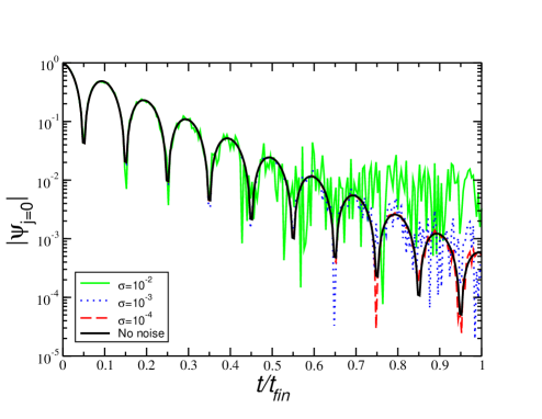
For illustration, in Fig. 3 we show a typical waveform generated in this way. The “true” signal (with $\sigma=0$) corresponds to a perturbed Schwarzschild black hole, i.e. the frequency and damping time correspond to the fundamental $l=m=2$ QNM for a black hole of dimensionless spin parameter $j=0$ bcw . For any given $\sigma$, the addition of Gaussian white noise has a less severe impact for large values of $j$. The reason is that the damping time of the $l=m=2$ mode grows with the rotation parameter $j$ (see eg. Table II in bcw ). A Schwarzschild waveform with $\sigma=10^{-3}$ is quite similar to the typical merger waveforms of Fig. 1, and for this reason we will use it to test the performance of the different fitting routines. Results for different values of $\sigma$ are qualitatively similar.

For each fitting algorithm, we perform Monte Carlo simulations to produce a large number ($N_{\rm noise}=100$) of realizations of the noise with $\sigma=10^{-3}$. For each realization of the noise ($\nu=1,\dots,N_{\rm noise}$) we fit the waveform varying the starting time from $t_{0}=0$ to $t_{0}=t_{\rm fin}$. Each fit yields a couple of values $\omega_{\nu}(t_{0}),~{}\alpha_{\nu}(t_{0})$, and from these we can deduce the quality factor of the oscillation $Q_{\nu}(t_{0})\equiv|\omega_{\nu}(t_{0})/[2\alpha_{\nu}(t_{0})]|$ bcw . For each $t_{0}$ we compute the standard deviation and bias of each of these fitted quantities $x$ ($=\omega,~{}\alpha$ or $Q$) from our Monte Carlo simulations:

$$\left.{\rm std}(x)\right|_{t_{0}} = \left\{\frac{1}{{N_{\rm noise}-1}}\sum_{\nu=1}^{N_{\rm noise}}[x_{\nu}(t_{0})-\bar{x}(t_{0})]^{2}\right\}^{1/2}\,,$$ (95)

$$\left.{\rm bias}(x)\right|_{t_{0}} = \bar{x}(t_{0})-x_{\rm true}\,,$$ (96)

where $x_{\rm true}$ is the known, true value of each quantity and a bar denotes the average over all noise realizations:

$$\bar{x}(t_{0})=\left[\frac{1}{N_{\rm noise}}\sum_{\nu=1}^{N_{\rm noise}}x_{\nu}(t_{0})\right]\,.$$ (97)

Figure 4: Standard deviation (left) and bias (right) in the estimate of frequency, damping time and quality factor (top to bottom). All quantities are given as functions of the starting time of the fit $t_{0}$ (normalized by the duration of the signal $t_{\rm fin}$); each point is the result of a Monte Carlo simulation obtained by adding $N_{\rm noise}=100$ realizations of Gaussian white noise with zero mean and $\sigma=10^{-3}$ to the $j=0$ waveform of Fig. 3. Solid (black), dashed (red) and dotted (blue) lines refer to the MP, KT and LM algorithms, respectively.

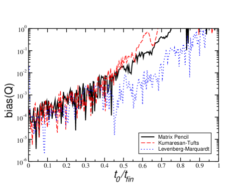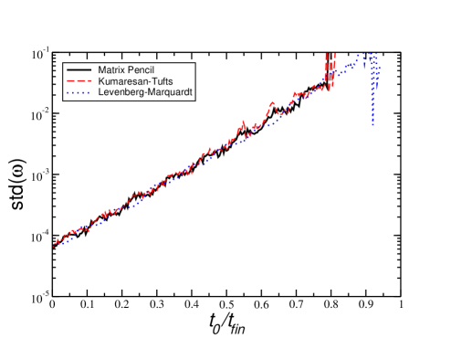
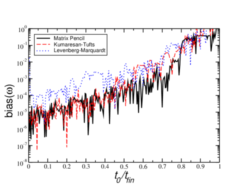
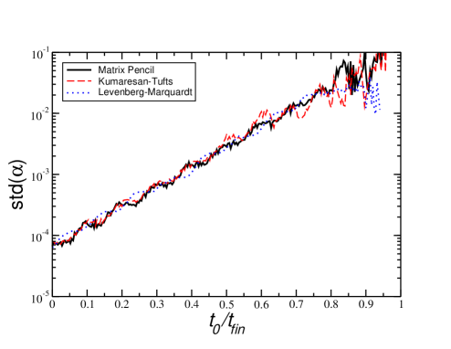
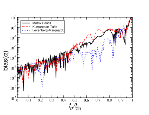
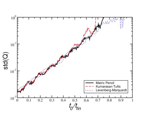
Results of these Monte Carlo simulations are shown in Fig. 4. There we see that all three methods (KT, MP and LM) are essentally equivalent in terms of variance. Standard deviation and bias grow sharply for $t_{0}/t_{\rm fin}\gtrsim 0.7$, when we are fitting that part of the signal which is buried in noise (compare Fig. 3). The bias is usually very small, but remarkably linear methods (KT, and especially MP) beat the non-linear LM fitting routine in terms of bias on the frequency. In terms of bias on the damping time, LM performs slightly better than MP and KT only for large values of $t_{0}$, when the SNR is very small.

When comparing the performance of the different methods it is useful to remember that LM only works if we give a good initial guess for the parameters we want to estimate, whereas MP and KT automatically find the values of these parameters, with no need for initial guesses. Our comparison is somehow “biased” in favour of the LM method in at least three ways: (i) we choose optimal initial guesses for the parameters, so that the LM algorithm is not “allowed” to converge to some wrong root; (ii) we choose a real signal rather than a complex signal, because the LM algorithm only works for real data sets; (iii) we only consider one damped exponential (LM often fails to converge if we include additional damped sinusoids, whereas Prony-type methods are still remarkably successful).

VI Application to merger waveforms

Here we turn to the problem that motivates the present analysis of fitting algorithms for complex exponentials in noise. If the ringdown radiation emitted as a result of a binary merger shows no signs of non-linearities or mode coupling, our fits should have a simple behavior: as we increase the starting time for the fit $t_{0}$, the black hole’s oscillation frequencies $\omega_{lmn}$ and damping factors $\alpha_{lmn}$ should asymptotically approach a constant, whose value is predicted by linear perturbation theory bcw .

Figure 5: Performance of different Prony methods in estimating the oscillation frequency $\omega$ (top) and damping factor $\alpha$ (bottom) for low and high-resolution runs (left and right, respectively). For concreteness we choose a binary with $q=1.5$ and consider the fundamental mode with $l=m=2$. Prony-type results refer to the complex waveform, while LM results are obtained by fitting the real part of the waveform only.

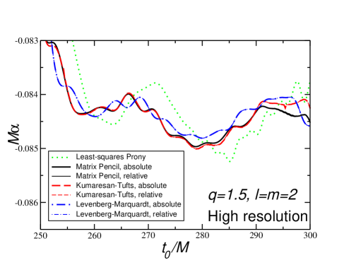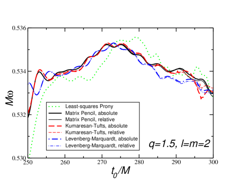
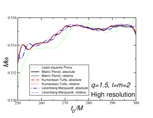
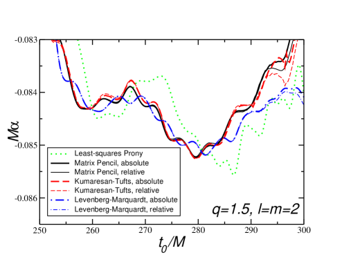
In Fig. 5 we show results of QNM fits performed on the $l=m=2$ component of low-resolution and high-resolution merger simulations with mass ratio $q=1.5$. Solid lines refer to the “absolute” truncation criterion of Section II, and dashed lines to the “relative” truncation criterion. Different truncation criteria affect the estimated parameters only for low-resolution simulations, and at late starting times ($t_{0}/M\gtrsim 290$). Results obtained fitting by a single complex exponential with standard least-squares Prony are slightly off from the “best” fitting methods (MP, KT and LM). Not surprisingly, there is remarkable agreement between KT and MP methods, and very good agreement between these two methods and the non-linear least-squares LM fit.

The main conclusion to be drawn from Fig. 5 is that all fitting routines consistently predict that frequencies and damping times have small (but non-trivial in structure) time variations. Relative variations in $\omega$ are of order $\sim 0.5\%$, with the frequency reaching a local maximum at $t_{0}/M\sim 272$. Relative variations in $\alpha$ are slightly larger (roughly $\sim 2.5\%$), with $|\alpha|$ attaining a maximum (and the damping time correspondingly attaining a minimum) for $t_{0}/M\sim 280$. Notice also that increasing the resolution sensibly reduces the irregularities in the predicted frequency at all times, and produces a flattening of the estimated parameters for $280\lesssim t_{0}/M\lesssim 300$. The decrease in $\omega$ and in $|\alpha|$ for $280\lesssim t_{0}/M\lesssim 300$, that are visible in the left panels, are clearly an artifact of insufficient resolution. It would be interesting to perform Richardson extrapolation of the numerical results to determine if oscillations in the estimated parameters (which could be a sign of “new” physics) disappear in the limit of infinite resolution. We plan to address this problem in the near future. An analysis of the fine structure of the signal, and of its implications for gravitational wave phenomenology, will be presented in a forthcoming publication follow-ups .

For the time being, we simply point out that such systematic variations in the oscillation frequency and/or damping time could be signs of non-linearities and/or mode coupling in the numerical simulations. Variations could be due to the black hole’s mass and angular momentum changing on a timescale which is longer than the QNM oscillation period, or to beating phenomena with other QNM frequencies. In our opinion, the fact that all fitting methods consistently predict the same “global” structure is convincing evidence that the existence of maxima and minima is not due to numerical errors in the fit.

Figure 6: Same as Fig. 5, but for the quality factor $Q$.

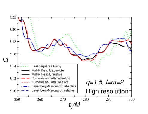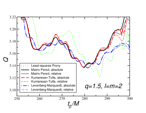
In Fig. 6 we plot the quality factor of the oscillations as a function of $t_{0}/M$. The time variation of $Q$ is basically dominated by the time variation of $\alpha$. This is quite obvious, since $Q=\omega/(2\alpha)$ and time variations in $\alpha$ are larger than time variations in $\omega$. The interest of plotting $Q(t_{0}/M)$ comes from the fact that, in linear theory and for $l=m$, $Q$ is a monotonic function of $j$ bcw . Roughly speaking, large variations in $Q$ for the fundamental oscillation mode could mean that the Kerr angular momentum parameter is changing in time, or that there are significant corrections to the linear approximation.

Figure 7: Oscillation frequency (top) and quality factor (bottom) for modes with $l=m=2$ and for low and high-resolution runs (left and right, respectively), as a function of the starting time of the fit. Thick lines use MP, thin lines use LM. Values of the quality factor for $t/M\lesssim 250$ are often unphysically large. We truncate the waveform at late times when the absolute value of the amplitude drops below $10^{-4}$ (for low resolution) or $10^{-5}$ (for high resolution). In each panel, lines from top to bottom refer to $q=1.0,~{}1.5,~{}2.0,~{}2.5,~{}3.0,~{}3.5,~{}4.0$.

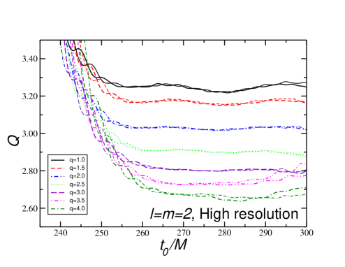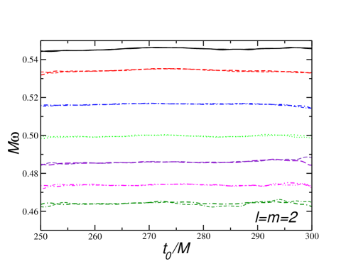
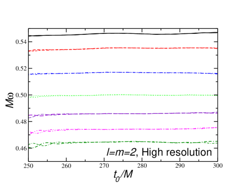
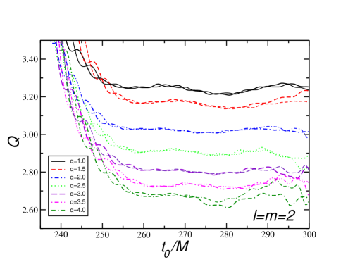
Finally, in Fig. 7 we compare the performance of our two “best” fitting methods (MP and LM) in estimating oscillation frequencies and quality factors for different mass ratios: $q=1.0,~{}1.5,~{}2.0,~{}2.5,~{}3.0,~{}3.5,~{}4.0$. Deviations in $Q$ between the two methods are quite significant, especially for large mass ratio, when the numerical simulations are less reliable. For $q=4.0$ and low resolution, the LM method shows larger variations in $\omega$ than the MP method. This could be an effect of the larger bias in frequency of the LM method, as compared with the MP method (cf. Fig. 4). Once again, increasing the resolution produces a flattening of all curves, the effect being more pronounced for large mass ratios. A more systematic analysis of simulations for different mass ratios will appear elsewhere follow-ups .

VII Conclusions and outlook

Our understanding of binary black hole mergers has recently been revolutionized by the success of numerical relativity simulations. A partial disappointment came from the remarkable simplicity of the inspiral-merger-ringdown transition: the non-linearities of Einstein’s theory do not seem to leave spectacular imprints on the merger, that seems to be a very short phase smoothly connecting the familiar “inspiral” and “ringdown” waveforms Buonanno:2006ui .

In this paper we argued that non-linearities could show up in the fine structure of the ringdown waveform, as systematic time variations of the ringdown frequencies and damping times. We also showed by explicit calculations that such time variations are actually present in numerical waveforms (see Figs. 5, 6 and 7). The variations we are looking for are typically $\sim 100$ times smaller than the QNM frequencies themselves. This smallness calls for accurate parameter estimation methods to extract ringdown frequencies from numerical simulations. We considered a class of well-studied and robust parameter estimation methods for complex exponentials in noise, which are modern variations of a linear parameter estimation technique first introduced in 1795 by Prony.

The comparison of different fitting methods can help resolve actual physical effects from systematic parameter estimation errors, due to the variance and bias of each particular fitting algorithm. For this reason we compared two variants of the original Prony algorithm (the Kumaresan-Tufts and matrix pencil methods kumaresantufts ; matrixpencil ) against standard non-linear least-squares techniques, such as the Levenberg-Marquardt algorithm. We found that the two classes of methods have comparable variance, but Prony-type methods tend to have slightly smaller bias. Prony methods have a number of advantages with respect to standard non-linear least-squares techniques:

• They do not require an initial guess of the fitting parameters.

• They provide us with a simple, efficient way to estimate QNM frequencies for the overtones, and even to estimate how many overtones are present in the signal reddybiradar ; waxkailath .

• They are explicitly designed to deal with complex signals, so they should be most useful for “generic” waveforms, such as those produced by spinning, precessing black hole binaries. In the case of non-trivial polarization of the gravitational radiation it might become crucial to fit simultaneously the real and imaginary parts of the signal to exploit optimally the information carried by both degrees of freedom.

• Statistical properties of Prony-based methods in the presence of noise (such as their variance and bias) are well studied and under control. Our Monte Carlo simulations suggest that the statistical properties of Prony-like methods as we vary the SNR are more consistent than for non-linear least-squares methods, even when we consider a single damped sinusoid (the dotted blue lines in Fig. 4 have a very irregular behavior).

The methods introduced in this paper should be useful both theoretically and experimentally. From a theoretical standpoint, besides helping in the search for non-linearities, Prony methods can also be used as “diagnostic tools” for numerical simulations. For example, monitoring the time variation of ringdown parameters from different multipolar components of the radiation we can check that the end-product of a merger is indeed consistent with the Kerr solution. An analysis of presently available numerical waveforms based on Prony methods is ongoing follow-ups .

So far, Prony algorithms have generally been overlooked by the GW data analysis community. We believe that the techniques presented in this paper should prove useful to extract science from noisy ringdown signals in the (hopefully not too distant) future, when GW detection will finally become a reality.

References

- (1) B. Brügmann, W. Tichy and N. Jansen, Phys. Rev. Lett. 92, 211101 (2004) [arXiv:gr-qc/0312112].
- (2) F. Pretorius, Phys. Rev. Lett. 95, 121101 (2005) [arXiv:gr-qc/0507014].
- (3) M. Campanelli, C. O. Lousto, P. Marronetti, and Y. Zlochower, Phys. Rev. Lett. 96, 111101 (2006) [arXiv:gr-qc/0511048].
- (4) J. G. Baker, J. Centrella, D.-I. Choi, M. Koppitz, and J. van Meter, Phys. Rev. Lett. 96, 111102 (2006) [arXiv:gr-qc/0511103].
- (5) F. Herrmann, D. Shoemaker and P. Laguna, arXiv:gr-qc/0601026.
- (6) U. Sperhake, arXiv:gr-qc/0606079.
- (7) M. A. Scheel, H. P. Pfeiffer, L. Lindblom, L. E. Kidder, O. Rinne and S. A. Teukolsky, Phys. Rev. D 74, 104006 (2006) [arXiv:gr-qc/0607056].
- (8) B. Brügmann, J. A. Gonzalez, M. Hannam, S. Husa, U. Sperhake and W. Tichy, arXiv:gr-qc/0610128.
- (9) J. A. Gonzalez, U. Sperhake, B. Brügmann, M. Hannam and S. Husa, arXiv:gr-qc/0610154.
- (10) B. Szilagyi, D. Pollney, L. Rezzolla, J. Thornburg and J. Winicour, arXiv:gr-qc/0612150.
- (11) E. Berti, S. Iyer and C. M. Will, Phys. Rev. D 74, 061503 (2006) [arXiv:gr-qc/0607047].
- (12) A. Buonanno, G. B. Cook and F. Pretorius, arXiv:gr-qc/0610122.
- (13) J. G. Baker, J. R. van Meter, S. T. McWilliams, J. Centrella and B. J. Kelly, arXiv:gr-qc/0612024.
- (14) K. D. Kokkotas and B. F. Schutz, Gen. Rel. Grav. 18, 913 (1986); K. D. Kokkotas and B. F. Schutz, Mon. Not. Roy. Astron. Soc. 225, 119 (1992).
- (15) C. V. Vishveshwara, Nature 227, 936 (1970); S. Chandrasekhar and S. Detweiler, Proc. R. Soc. London A344, 441 (1975); K. D. Kokkotas and B. G. Schmidt, Living Rev. Rel. 2, 2 (1999); H.-P. Nollert, Class. Quantum Grav. 16, R159 (1999).
- (16) E. W. Leaver, Proc. Roy. Soc. Lond. A 402, 285 (1985).
- (17) E. Berti, V. Cardoso and C. M. Will, Phys. Rev. D 73, 064030 (2006).
- (18) Y. Zlochower, R. Gomez, S. Husa, L. Lehner and J. Winicour, Phys. Rev. D 68, 084014 (2003) [arXiv:gr-qc/0306098].
- (19) E. Berti, V. Cardoso and M. Casals, Phys. Rev. D 73, 024013 (2006) [Erratum-ibid. D 73, 109902 (2006)] [arXiv:gr-qc/0511111].
- (20) E. N. Dorband, E. Berti, P. Diener, E. Schnetter and M. Tiglio, Phys. Rev. D 74, 084028 (2006) [arXiv:gr-qc/0608091].
- (21) R. Boyer and J. Rosier, Proc. of the Int. Conference on Digital Audio Effects (2002); K. Hermusa, W. Verhelstb, P. Lemmerlingc, P. Wambacq, S. Van Huffel, Signal processing 85(1), 163 (2005).
- (22) M. Wax and T. Kailath, IEEE Trans. Acoust., Speech, Signal Processing 33 (2), 387 (1985); J. J. Fuchs, IEEE Trans. Acoust., Speech, Signal Processing 36 (12), 1846 (1988).
- (23) A. I. Kul ment ev, Eur. Phys. J. Appl. Phys. 25, 191 (2004).
- (24) E.-H. Djermoune, Estimation des paramètres de sinusoides amorties par décomposition en sous-bandes adaptative. Application à la spectroscopie RMN, PhD thesis (Centre de Recherche en Automatique de Nancy, Université Henri Poincarè, 2003, unpublished).
- (25) S. L. Marple, Digital spectral analysis with applications, (Prentice-Hall, New Jersey, 1987).
- (26) R. N. McDonough and W. H Huggins, IEEE Trans. Autom. Control AC-13, 408 (1968); A. G. Evans and R. Fischl, IEEE Trans. Aerosp. Electron. Syst. AES-12, 583 (1976).
- (27) G. de Prony, Journal de l’École Polytechnique 1(2), 24 (1795).
- (28) R. Kumaresan and D. W. Tufts, IEEE Transaction on Acoustics, Speech and Signal Processing 30 (6), 833 (1982); D. W. Tufts and R. Kumaresan, Proceedings of the IEEE 70 (9), 975 (1982).
- (29) Y. Hua and T. K. Sarkar, IEEE Transaction on Acoustics, Speech and Signal Processing 38 (5), 814 (1990); T. K. Sarkar and O. Pereira, IEEE Antennas and Propagation Magazine 37(1), 48 (1995).
- (30) E. Berti, V. Cardoso, J. A. Gonzalez, U. Sperhake, M. Hannam, S. Husa and B. Brügmann, gr-qc/0703053.
- (31) J. G. Baker, M. Campanelli, C. O. Lousto and R. Takahashi, Phys. Rev. D 65, 124012 (2002) [arXiv:astro-ph/0202469].
- (32) E. Berti and V. Cardoso, Phys. Rev. D 74, 104020 (2006) [arXiv:gr-qc/0605118].
- (33) R. H. Price, Phys. Rev. D 5, 2419 (1972).
- (34) K. Levenberg, Quart. Appl. Math. 2, 164 (1944); D. Marquardt, SIAM J. Appl. Math. 11, 431 (1963).
- (35) J. J. Mor , D. C. Sorensen, K. E. Hillstrom, and B. S. Garbow, “The MINPACK Project,” in Sources and Development of Mathematical Software, W. J. Cowell, ed., Prentice-Hall, pp. 88-111 (1984).
- (36) http://www.wolfram.com/products/mathematica/index.html
- (37) S. Marcos, Les méthodes à la haute résolution: traitment dántennes et analyse spectrale (Hermès, Paris, 1998).
- (38) M. A. Rahman and K.-B. Yu, IEEE Transaction on Acoustics, Speech and Signal Processing 35 (10), 1440 (1987).
- (39) A. C. Kot, S. Parthasarathy, D. W. Tufts and R. J. Vaccaro, in Proceedings of the International Conference on Acoustics, Speech and Signal Processing, 1549 (1987).
- (40) B. Porat and B. Friedlander, IEEE Transaction on Acoustics, Speech and Signal Processing 35 (2), 231 (1987); Y. Hua and T. K. Sarkar, IEEE Transaction on Acoustics, Speech and Signal Processing 36 (2), 228 (1988); A. Okhovat and J. R. Cruz, in Proceedings of the International Conference on Acoustics, Speech and Signal Processing, 2286 (1989).
- (41) E.-H. Djermoune and M. Tomczak, 12th European Signal Processing Conference (EUSIPCO’04), Wien, Austria (2004).
- (42) B. Porat, Digital processing of random signal: theory and methods (Prentice Hall Information and System Sciences Series, 1993).
- (43) J. C.Hamann and S. Singh, http://www.engr.uconn.edu/~sas03013/pronytool/prony.html
- (44) C. Pozrikidis, http://dehesa.freeshell.org/SOFT/FDLIB/FDLIB/08_stab/prony/
- (45) G. Smyth, http://www.statsci.org/other/prony.html
- (46) J. H. McClellan, C. Sidney Burrus, A. V. Oppenheim, T. W. Parks, R. W. Schafer, H. W. Schuessessler, Computer Based Exercises for Signal Processing using MATLAB (Prentice Hall, 1997).
- (47) V. U. Reddy and L. S. Biradar, IEEE Transactions on Signal Processing, bf 41, 2872 (1993).
- (48) M. Wax and T. Kailath, IEEE Transactions on Acoustics, Speech and Signal Processing, ASSP-33, 387 (1985).
- (49) E.-H. Djermoune and M. Tomczak, 11th European Signal and Image Processing Conference (EUSIPCO’02), 139, Toulouse, France (2002).
- (50) G. E. P. Box and M. E. Muller, Ann. Math. Stat. 29, 610 (1958).
- (51) W. H. Press, S. A. Teukolsky, W. T. Vetterling and B. P. Flannery, Numerical Recipes in Fortran, Second Edition (Cambridge University Press, Cambridge, 1992).