Shedding Some New Lights upon the Stellar Quasi-Normal Modes

Abstract

In the current paper we present some new data on the issue of quasi-normal modes (QNMs) of uniform, neutron and quark stars. These questions have already been addressed in the literature before, but we have found some interesting features that have not been discussed so far. We have increased the range of frequency values for the scalar and axial perturbations of such stars and made a comparison between such QNMs and those of the very well-known Schwarzschild black holes. Also addressed in this work was the interesting feature of competing modes, which appear not only for uniform stars, but for quark stars as well.

I Introduction

Quasi normal modes (QNM’s) have been studied for quite a long time due to the possibility of gathering information from astrophysical objects in terms of their response to external perturbations, in the same sense as we may study a bell from its sound. For reviews and earlier notes see Chand-Ferr , Kokkotas , Price . They are particularly useful to grasp also general properties of the metric under consideration - see WMA , WLA , Kar .

Stellar QNM’s have been under considerable scrutiny over the last decades, since they provide not only a test for Einstein’s theory of General Relativity (GR), but also a look into the stellar structure and, indirectly, into the very nature of stellar matter and its properties, such as its equation of state (EOS).

Stars have an internal structure which must be accounted for when studying any kind of perturbation, be it a test scalar field or a gravitational perturbation. Among these, the axial perturbations are much easier to compute, since they do not mix with the fluid modes of the star Chand-FerrB . Such axial perturbations (along with the scalar and electromagnetic) can be described by a wave equation of the form

$$-\frac{\partial^{2}W}{\partial t^{2}}+\frac{\partial^{2}W}{\partial x^{2}}=VW,$$ (1)

where $W$ stands for the amplitude and $V$, for the perturbative potential. For details, see the Appendix.

The polar perturbations mix with the fluid modes and require a completely different approach in their numerical analysis and evolution, and are not dealt with here.

Uniform stars, that is, stars possessing a uniform density $\varepsilon=\varepsilon_{0}$ are idealized astrophysical objects, since they cannot exist in nature. Unrealistic as they may sound, though, such stars provide an interesting background in which some insight on the field dynamics in stellar geometries may be gained, since the physical quantities of relevance (mass, pressure and gravitational potentials of the metric) are very straightforward to evaluate. We begin with such stars, but we do not limit ourselves to them. We present some results for the neutron and quark stars and compare these results to those of the well-known Schwarzschild black holes.

For the neutron stars, we have dealt with the simplest model available, that of Oppenheimer and Volkov OV-39 , consisting of a pure Fermi gas of neutrons. For the quark stars, we have also used one of the simplest models available, the MIT Bag Model.

In this paper we consider QNMs of uniform, neutron and quark stars and compare with the analogous results for black holes, in an attempt to describe properties inherent of astrophysical objects.

In section II we present some results about uniform stars. Within that section, the question of secondary modes in such stars is discussed. In section III, we discuss neutron star QNMs and in section IV we do the same for quark stars. Comparative charts for all QNMs are available in section V and the remarks and conclusions are left for section VI.

Concerning units, we have used the geometric system of units, for which $\hbar=c=G=1$. This means that the masses have dimension of length and are measured in metres. The conversion factor from metres to kilograms is $c^{2}/G$. Before proceeding, we just recall a definition which will be very useful throughout this paper, that of compactness of a star. The compactness $c$ for a spherically symmetric star is defined in the literature as

$$c=\frac{r_{g}}{R},$$ (2)

in which $r_{g}=2M$ is the star’s gravitational radius and $R$ is its actual radius.

II QNMs of Uniform Stars - Some Results

We begin with a series of figures - from the data we have tabulated - on the frequencies of the QNMs for uniform stars, with some of the masses we have chosen for neutron and quark stars, namely $M=1048m$, $M=977m$, $M=665m$ and $M=330m$ (the first two were also used for neutron and quark stars), for the sake of comparison. One must bear in mind that such values are not special in any way, being just the results of star integrations for some particular choices of the central density $\varepsilon_{0}$, and even these latter choices are just choices - for more details on the matter, see section III. In what follows, $c$ stands for the compactness of the star, $\ell$ for the multipole index and $\omega_{R}$ and $\omega_{I}$ for the real and the imaginary part of the frequency, respectively.

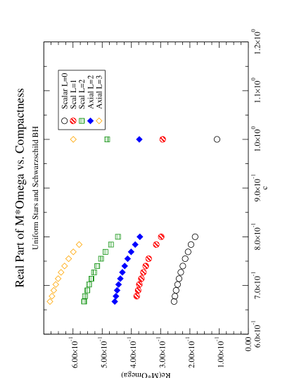
Figure 1: QNM frequencies (real part) for a uniform star, various fields, changing compactness. The $c=1$ mark is for the Schwarzschild BH.

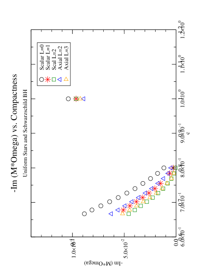
Figure 2: QNMs frequencies (negative of the imaginary part) for a uniform star, various fields, changing compactness. The $c=1$ mark is for the Schwarzschild BH.

From the data we have compiled, we can make a few initial remarks. First, we have noticed that $\omega\propto\frac{1}{M}$, as in the pure Schwarzschild case. Such a scaling property for $\omega$ in uniform stars was also explored in this work, and more data are left for subsection B. Second, increases of $\omega_{R}$ with $\ell$ (as expected). Moreover, all axial frequencies have smaller real parts than their scalar counterparts, given some $\ell$ (exactly like Schwarzschild). But $-\omega_{I}$ is higher for axial perturbations than for scalar ones (in contrast to the Schwarzschild case).

We shall illustrate our data with a set of graphics. We begin with the picture for the scalar $\ell=0$ case, which can be viewed in Fig. (3).

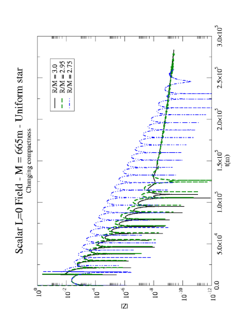
Figure 3: QNMs for a uniform compact star. Scalar $\ell=0$ case shown. $M=665m$.

In Fig. (3), the tail obeys a power-law, namely $t^{-4}$. A comparison between uniform star and Schwarzschild BH modes for the $\ell=0$ scalar field is provided in Fig. (4). Notice that the BH-background scalar field oscillates much less than in uniform stars, although the tail decays much in the same way, according to the same power law.

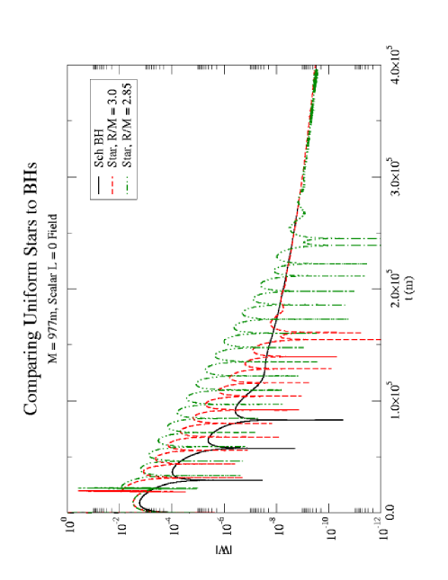
Figure 4: QNMs and tails for stars and Schwarzschild BHs. Scalar $\ell=0$ case shown. $M=977m$. The tails have the same qualitative behaviour.

II.1 QNM Overtones

We have detected, throughout our investigation of compact uniform stars, the presence of secondary modes which decay faster than the dominant ones. Since we have seen a similar behavior in the Schwarzschild BH context (see note at the end of this subsection) and we have checked these Schwarzschild BH data and concluded that they correspond to the first overtones, we can speak of overtones of the fundamental modes in the stellar context, also.

These overtones show themselves in the form of wiggles in the envelopes of the Misner curves characterising the QNMs, as if there were modes (actually, the overtones) competing with the dominant ones. This issue of competing modes deserves special attention, especially for - but not limiting to - high compactnesses ($c>0.76$), when these wiggles become clearer. Three examples of competing modes are provided in Figs. (5), (6) and (7).

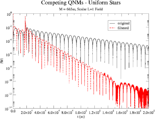
Figure 5: Competing QNMs for a uniform compact star, $c=0.741$. Scalar $\ell=1$, $M=665m$ case shown. The secondary mode decays much faster.

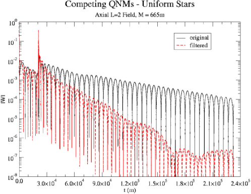
Figure 6: Competing QNMs for a uniform compact star, $c=0.769$. Axial $\ell=2$, $M=665m$ case shown.

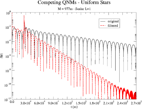
Figure 7: Competing QNMs for a uniform compact star, $c=0.741$. Scalar $\ell=1$, $M=977m$ case shown.

A comment is due on the method of extraction of such secondary modes: we have fitted a damped oscillating function to the original data, so that we could know the frequency $\omega$ of the dominant mode (the one with the weaker damping) - visible at the end of the time evolution in all figures - and subtracted the fitted function from the original data. The remaining mode is the competing mode we have just talked about. For some extra details on the method, see dgiugno-06 .

Our fittings are not always very precise, so that we give no more than 3 significant figures for them, in the dominant mode. The remaining mode is not always very easy to fit, primarily due to these precision limitations. This remaining mode may look as if it were trembling, but in some cases we can still made a (quite poor) fitting to it. We expect it to have a stronger - usually much stronger - decay, which was indeed the case.

In the few cases in which we have seen a somewhat clear secondary mode, we could notice also a slightly faster oscillation. For the modes seen on Fig. (5) we have, for instance, $M\omega=0.351-0.0204i$ for the dominant mode and $M\omega=0.47-0.087i$ for the secondary mode, whereas for those seen on Fig. (6) we have $M\omega=0.401-0.0120i$ for the dominant mode and $M\omega=0.49-0.042i$ for the competing mode, so that the latter has a much stronger decay. The number of significant figures for the latter was also reduced, since it was obtained after a three-figure fitting had been performed. More data are available in Table (1), for $\frac{R}{M}=2.6$.

These data simply confirm what we have said about the secondary modes in question: they oscillate somewhat faster (in contrast to their Schwarzschild counterparts) and decay much faster than the dominant ones (similarly to the Schwarzschild BH case). This behaviour is confirmed in Table (2), where the relation between the real and imaginary parts of $\omega$ for the dominant and the secondary modes is shown (for the scalar $\ell=1$ field and $M=977m$). The oscillations are about 30% faster for the secondary modes and this percentage seems to have a weak - if any - correlation to the compactness $c$, but the damping rates can be at least 4 times higher for the secondary modes, and sometimes up to 9 times, increasing sharply with $c$. For the Schwarzschild BH, at least for the $\ell=2$ and $\ell=3$ axial cases, the decay rate was around 3 times faster for the competing mode (the first overtone). As for the first overtones, we could see that $\omega_{R}\propto\frac{1}{M}$, but for $\omega_{I}$ the data seemed to fluctuate somewhat. This may be due to the fitting precision limitations to which we have referred earlier. See table (1).

$Mass(m)$	$field$	$\ell$	$M\omega^{DOM}$	$M\omega^{SEC}_{I}$
$1048$	$scal$	$1$	$0.329-0.0102i$	$0.42-0.056i$
$1048$	$axial$	$2$	$0.401-0.0121i$	$0.49-0.046i$
$977$	$scal$	$1$	$0.329-0.0102i$	$0.42-0.053i$
$977$	$axial$	$2$	$0.402-0.0120i$	$0.49-0.050i$
$665$	$scal$	$1$	$0.329-0.0102i$	$0.43-0.055i$
$665$	$axial$	$2$	$0.401-0.0120i$	$0.49-0.042i$

Table 1: Comparing dominant ($\omega^{DOM}$) and competing ($\omega^{SEC}$) mode frequencies for several masses of uniform stars with $R/M=2.6$ ($c=0.769$).

$c$	$M\omega^{DOM}_{R}$	$-M\omega^{DOM}_{I}$	$M\omega^{SEC}_{R}$	$-M\omega^{DOM}_{I}$	$\frac{\omega^{SEC}_{R}}{\omega^{DOM}_{R}}$	$\frac{\omega^{SEC}_{I}}{\omega^{DOM}_{I}}$
$0.727$	$0.359$	$0.0262$	$0.48$	$0.11$	$1.3$	$4.2$
$0.741$	$0.351$	$0.0204$	$0.47$	$0.087$	$1.3$	$4.3$
$0.755$	$0.341$	$0.0150$	$0.45$	$0.073$	$1.3$	$4.9$
$0.769$	$0.329$	$0.0102$	$0.43$	$0.055$	$1.3$	$5.4$
$0.784$	$0.316$	$0.00608$	$0.40$	$0.042$	$1.3$	$6.9$
$0.800$	$0.298$	$0.00272$	$0.39$	$0.025$	$1.3$	$9.2$

Table 2: Comparing dominant and secondary modes for the $\ell=1$ scalar field, for a uniform star with mass $M=665m$.

A brief remark on the Schwarzschild BH case: it is well-known Kokkotas that in their context, secondary modes (or first overtones) may indeed appear. The same holds for higher overtones. We have searched for them in the same context in order to test the procedure we have adopted to extract secondary modes from uniform compact stars. The data we got for the axial $\ell=2$ axial field, for instance, were compared to those of Kokkotas and we have found a good agreement between our results and theirs, indicating that our method, however simple-minded as it seems, may indeed yield interesting results. To be more precise, for the $n=0$ mode (the fundamental), they got $M\omega=0.37367-0.08896i$, the same as ours. For the first overtone ($n=1$) they had $M\omega=0.34671-0.27391i$ and we had $M\omega=0.352-0.272i$ for $M=1048m$. This agreement is not so good as that for the $n=0$ mode, but seems to be good enough for us, indicating that our numerical procedures are on the right track. No higher overtones ($n>1$) were detected in the present context. Again, see dgiugno-06 for closer details.

From the last paragraph, we may conclude that the first overtones decay faster in both the Schwarzschild case and the uniform compact star case, though in the latter case the decay rate depends on the compactness, being higher in more compact stars and usually higher than in the Schwarzschild context. One important difference between first overtones in Schwarzschild BHs and uniform stars backgrounds concerns their oscillations, which are slightly slower than in the fundamental mode for the former and somewhat faster (though not much) in the latter.

II.2 Scaling Properties and Other Comments

We can also check the dependence of the modes - for a given compactness and perturbation - on the mass, as shown in Fig. (8).

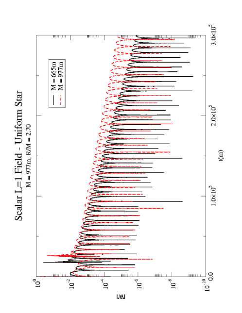
Figure 8: QNMs for a uniform compact star. The field oscillates and decays more slowly for a more massive star, exactly as one would expect from a Schwarzschild black hole.

Besides fig. (8), one may find an interesting scaling property for uniform star QNMs.

$Mass(m)$	$c$	$field$	$\ell$	$M\omega$
$1048$	$0.769$	$scal$	$1$	$0.329-0.0102i$
$1048$	$0.769$	$axial$	$2$	$0.401-0.0121i$
$977$	$0.769$	$scal$	$1$	$0.329-0.0102i$
$977$	$0.769$	$axial$	$2$	$0.402-0.0120i$
$665$	$0.769$	$scal$	$1$	$0.329-0.0102i$
$665$	$0.769$	$axial$	$2$	$0.401-0.0120i$
$1048$	$0.740$	$axial$	$2$	$0.422-0.0233i$
$977$	$0.740$	$axial$	$2$	$0.421-0.0234i$
$665$	$0.740$	$axial$	$2$	$0.423-0.0233i$
$977$	$0.769$	$scalar$	$2$	$0.489-0.00440i$
$665$	$0.769$	$scalar$	$2$	$0.489-0.00448i$

Table 3: Search for scaling properties of the QNM frequencies - Uniform Stars.

The table (3) shows that for a given field, compactness and $\ell$, the quantity $M\omega$ is practically constant. For instance, when $\ell=1$ for the scalar field and $c=0.769$ ($R/M=2.6$), one has $M\omega$ being $0.329-0.0102i$ for both $M=977m$ and $M=665m$, while for $c=0.740$ ($R/M=2.7$) one has $M\omega=0.351-0.0204i$ for $M=665m$, and almost the same ($M\omega=0.349-0.0205i$) for $M=977m$. This can be corroborated for a larger mass spectrum, different compactnesses, fields and $\ell$ values.

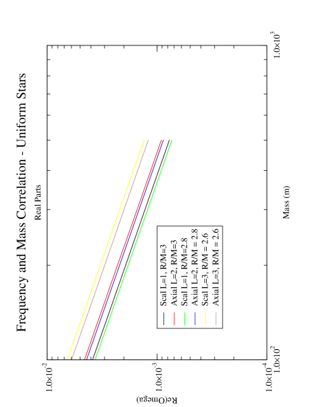
Figure 9: $\omega_{R}$ vs. the mass.

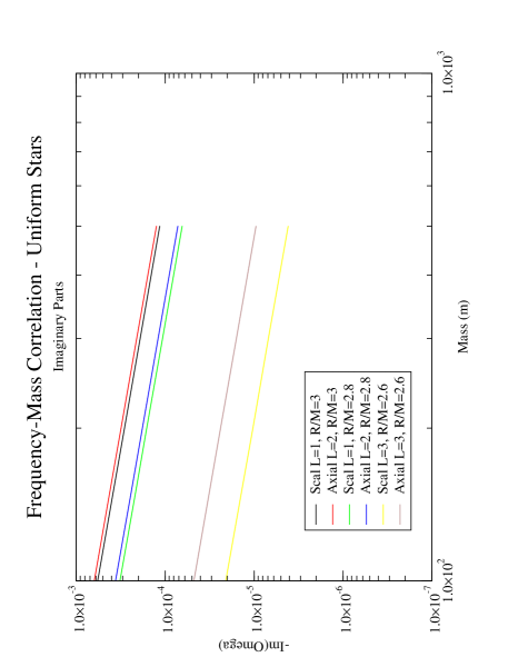
Figure 10: $-\omega_{I}$ vs. the mass.

III Neutron Stars

We have worked with the simplest model available for neutron stars, that of a noninteracting Fermi gas of neutrons. For those, the maximum mass is $0.72M_{s}$ Haensel , and we have selected a few values of neutron star masses to work with. For a brief description of the EOS involved, see Weinberg . Here we shall work on the QNMs and other features of the stellar perturbations. The masses we have selected for comparison with other kinds of stars were $M=1048m$, $M=977m$, $M=665m$ and $M=330m$. Such values are simply a matter of choice, having no special feature. They simply correspond to some particular choices of central density, $\varepsilon_{0}$, namely $4.0\cdot 10^{15}g/cm^{3}$, $1.5\cdot 10^{15}g/cm^{3}$, $3.0\cdot 10^{14}g/cm^{3}$ and $5.0\cdot 10^{13}g/cm^{3}$, respectively. These values, in turn, are also just a matter of choice. Further values could have been equally taken.

Some of our results are available in Figs. (11), (12) and (13).

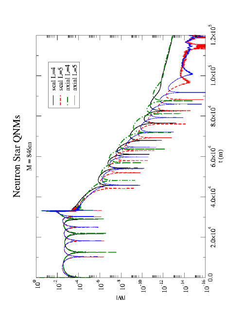
Figure 11: QNMs for the scalar and axial fields when $M=846m$, $\ell=4,5$.

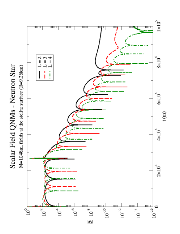
Figure 12: Scalar field QNMs when $M=1048m$, with changing $\ell$. As one would expect, fields oscillate faster for higher $\ell$.

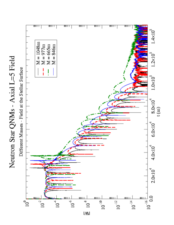
Figure 13: $\ell=5$ axial field, seen at the stellar surface. Several masses for neutron stars. Notice the increase in the oscillation rate with increasing $M$.

It would be interesting to compare these results to those coming from the Schwarzschild black hole QNM analysis. Some of our data on neutron stars can be seen in tables (4) and (5). These tables also display $M\omega$, and upon examining them we verify that the simple mass-frequency scaling property seen in the Schwarzschild BH and in the uniform star contexts did not show up here. The product $M\omega$ decreases with decreasing $M$, both for its real part and for the negative of its imaginary part.

$M(m)$	$\ell$	$\omega(\times 10^{-4})$	$M\omega$
$1048.25$	$2$	$3.78-2.86i$	$0.396-0.300i$
$1048.25$	$3$	$4.86-3.15i$	$0.509-0.330i$
$1048.25$	$4$	$5.91-3.58i$	$0.619-0.375i$
$1048.25$	$5$	$7.06-3.94i$	$0.740-0.413i$
$977.12$	$2$	$-$	$-$
$977.12$	$3$	$4.04-3.18i$	$0.395-0.311i$
$977.12$	$4$	$4.78-3.41i$	$0.467-0.333i$
$977.12$	$5$	$5.64-3.45i$	$0.551-0.337i$
$846.54$	$2$	$-$	$-$
$846.54$	$3$	$3.55-2.79i$	$0.300-0.236i$
$846.54$	$4$	$4.05-3.28i$	$0.343-0.277i$
$846.54$	$5$	$4.86-3.31i$	$0.411-0.280i$

Table 4: Frequency data on Neutron Stars, several masses, scalar field. Dashes indicate lack of reliable data. The $\ell=0,1$ modes showed very few oscillations before decaying to a power-law tail.

$Mass(m)$	$\ell$	$\omega^{surf}(\times 10^{-4})$	$M\omega$
$1048.25$	$2$	$2.81-2.49i$	$0.294-0.261i$
$1048.25$	$3$	$4.23-2.76i$	$0.443-0.289i$
$1048.25$	$4$	$5.61-3.45i$	$0.588-0.362i$
$1048.25$	$5$	$6.65-3.44i$	$0.697-0.361i$
$977.12$	$2$	$-$	$-$
$977.12$	$3$	$-$	$-$
$977.12$	$4$	$4.42-3.25i$	$0.432-0.318i$
$977.12$	$5$	$5.70-3.84i$	$0.557-0.372i$
$846.54$	$2$	$-$	$-$
$846.54$	$3$	$-$	$-$
$846.54$	$4$	$3.65-2.96i$	$0.309-0.250i$
$846.54$	$5$	$4.42-3.04i$	$0.374-0.257i$

Table 5: Frequency data on neutron stars. Axial field, different masses.

The corresponding frequencies for the Schwarzschild BH are available in Table (6). We have picked, for these, masses similar to those used for the neutron stars, and the data were taken from dgiugno-06 .

$field$	$\ell$	$M\omega$
$scalar$	$2$	$0.483644-0.0967590i$
$axial$	$2$	$0.37367-0.08896i$
$scalar$	$3$	$0.675367-0.0964997i$
$axial$	$3$	$0.599444-0.0927031i$
$scalar$	$4$	$0.867417-0.0963923i$
$axial$	$4$	$0.809180-0.0941643i$
$scalar$	$5$	$1.059614-0.0963337i$
$axial$	$5$	$1.012297-0.0948713i$

Table 6: QNM frequencies for the Schwarzschild BH, for the sake of comparison. We have chosen to show $M\omega$ due to the mass-frequency scaling property of such Schwarzschild BH modes.

The tables (4) and (5) show the stellar QNM frequencies obtained at the stellar surface. We must mention that the location of extraction - in the time domain - of the modes mattered in the final result, although it is not visible in tables (4) and (5), because we have taken average values, that is, the (arithmetic) average of several values measured at different time intervals. For example, for the case of a neutron star with $M=1048m$ and with an $\ell=4$ axial peturbation, we have gotten $\omega_{1}=5.55\cdot 10^{-4}-3.45\cdot 10^{-4}i$, $\omega_{2}=5.47\cdot 10^{-4}-3.32\cdot 10^{-4}i$ and $\omega_{3}=5.53\cdot 10^{-4}-3.39\cdot 10^{-4}i$ for the time intervals $t_{1}=60000-90000m$, $t_{2}=65000-85000m$ and $t_{3}=61000-91000m$, respectively, yielding an average value of $\omega=5.52\cdot 10^{-4}-3.39\cdot 10^{-4}i$. Similar variations were also seen for other $M,\ell$ values and fields. A similar phenomenon also happened for quark stars, although in a less pronounced way. No clear overtones were found in the neutron star context, while - in a few cases only - we could clearly find them in the quark star context (see next section).

From tables (4) and (5), we can draw a few conclusions. First, the axial modes have oscillated slowlier than their scalar counterparts, exactly as in the Schwarzschild BH case. But what has caught our attention, in fact, was the behavior of the oscillation rate ($Re(\omega)$) of the modes as a function of the stellar mass: the smaller the latter, the smaller the former, contrary to what is observed in the Schwarzschild case. More data are needed to clarify the matter.

Upon comparing the tables (4) and (5) to table (6), we may say that neutron star QNMs (at least in this simplified model we have dealt with) oscillate more slowly and decay considerably faster than Schwarzschild’s, at least for the few cases which we were able to study.

IV Quark Stars

In what follows, we deal with the issue of searching for and analysing the QNMs of very simple quark stars. The ones we have searched for obeyed a very simple EOS - the so-called MIT Bag Model - in which the pressure $p$ is given by

$$p=\frac{1}{3}(\varepsilon-4B),$$ (3)

where $B$ stands for the bag constant. For more details on this model see Weber04 , Glendenning and references therein. For further models of quark stars, see Glendenning and Su .

Upon dealing with the present class of stars, first of all, we have searched for values of $\varepsilon_{0}$ and $B$ which yielded masses very near those we had gotten for our neutron stars. For those, our limiting mass was around $0.72M_{s}$ and, according to Witten , there is an empirical expression for the maximum mass for a given $B$, namely,

$$M_{max}=\frac{1.96M_{s}}{\sqrt{B/B_{c}}},$$ (4)

where $B_{c}=60MeV/fm^{3}$. In order to have $M_{max}=0.72M_{s}$, one must choose $B=445MeV/fm^{3}$. Once we have found that, we just determine - by trial and error - the central densities $\varepsilon_{0}$ which yield the masses we want.

Once the stars were integrated, we had all the data on the perturbative potentials, as we did for the uniform and neutron stars, and the QNM-searching routine could be started to find the modes.

For these stars, we have some results, which can be seen in Figs. (14) and (15). A comparison between quark and neutron star modes is provided in Fig. (16).

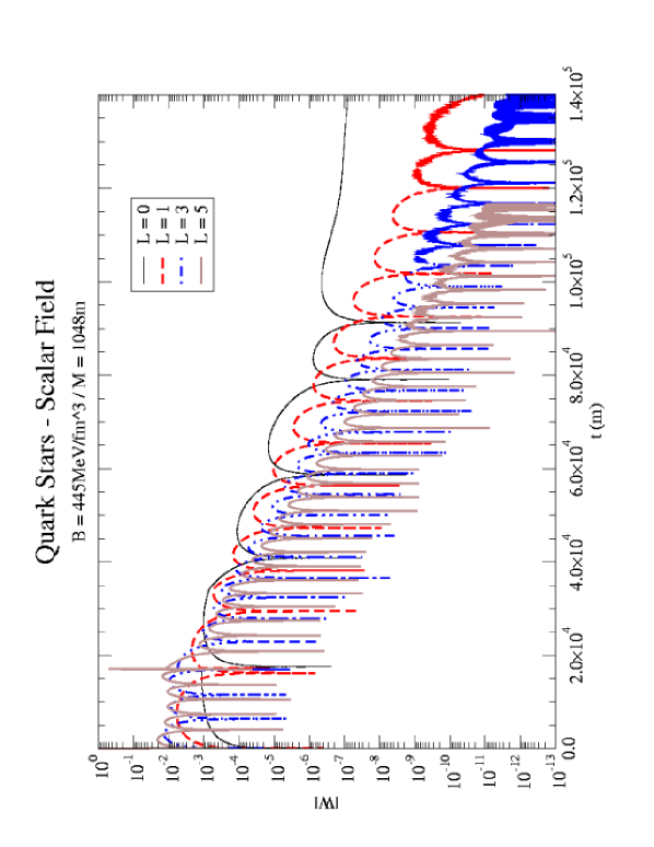
Figure 14: Scalar Field QNMs, Quark Stars, $B=445MeV/fm^{3}$ and $M=1048m$.

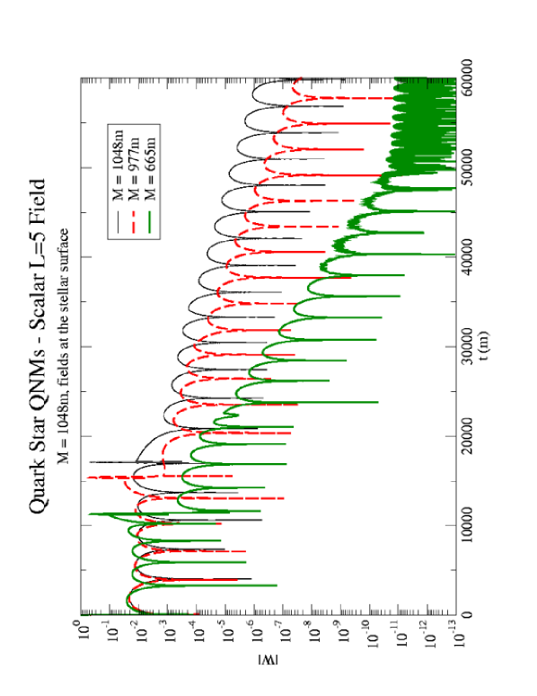
Figure 15: Scalar $\ell=5$ Field QNMs, Quark Stars, $B=445MeV/fm^{3}$ and different masses.

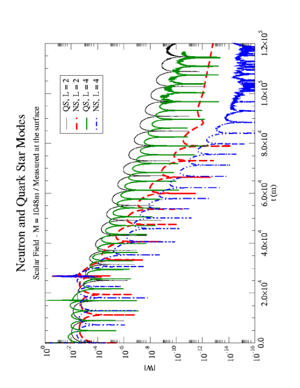
Figure 16: Comparing QNMs from Neutron and Quark Stars, $M=1048m$.

The figures above show that quark star modes, for a given mass, field type and $\ell$, oscillate considerably faster than neutron star modes, besides being less damped. Recall that the most massive neutron stars in this very simple model have a maximum mass of $1048m\thickapprox 0.72M_{s}$, and that they experience an increase in their oscillation rates for higher masses - just the opposite of quark stars. Thus, for any mass below this limit, neutron star modes will oscillate less than quark star modes.

$M(m)$	$\ell$	$\omega^{surf}(\times 10^{-4})$	$M\omega$
$1048$	$1$	$3.47-1.45i$	$0.364-0.152i$
$1048$	$2$	$5.26-1.63i$	$0.551-0.171i$
$1048$	$3$	$7.06-1.78i$	$0.740-0.187i$
$1048$	$4$	$8.85-1.92i$	$0.927-0.201i$
$1048$	$5$	$10.6-2.06i$	$1.11-0.216i$
$977$	$1$	$3.58-1.84i$	$0.350-0.180i$
$977$	$2$	$5.42-2.09i$	$0.530-0.204i$
$977$	$3$	$7.26-2.27i$	$0.709-0.220i$
$977$	$4$	$9.11-2.45i$	$0.890-0.239i$
$977$	$5$	$10.9-2.62i$	$1.06-0.254i$
$846$	$1$	$3.76-2.38i$	$0.318-0.201i$
$846$	$2$	$5.77-2.90i$	$0.488-0.245i$
$846$	$3$	$7.75-3.04i$	$0.656-0.257i$
$846$	$4$	$9.79-3.13i$	$0.828-0.265i$
$846$	$5$	$11.7-3.58i$	$0.990-0.303i$

Table 7: Frequency data for $B=445MeV/fm^{3}$ Quark Stars, several masses, scalar field. Dashes indicate the lack of reliable data.

As for our current data on the axial modes, they seemed not to be of good quality and we have yet to find out why.

One point should be stressed about the data in Table (7): as we had already commented on the neutron star context, depending on the region of the time domain used to make the fittings to find the QNM frequencies, the results differed a bit (not as much as for the neutron stars). We have decided to rely on the data obtained at the end of the time domain - because any overtone tends to show itself at the beginning of the wave profile - but before the onset of any instability (seen by the ’trembling’ data). After making such a fitting, we decided to subtract it from our original function (as we had done in dgiugno-06 , in another context). To our surprise, we could find a secondary mode in most cases, though only in a few cases it was possible to make a minimally reliable fitting to it. See Fig. (17).

An extra remark is due on the data in Table (7): we computed also $M\omega$, and we have not seen the same simple scaling property we had seen before for the Schwarzschild BH modes and for the uniform stars. The real part of $M\omega$ decreases with $M$, and the opposite holds for the imaginary part of $-M\omega$.

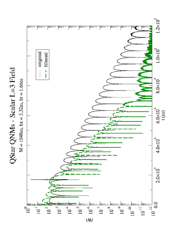
Figure 17: Scalar $\ell=3$ field, $M=1048m$. Notice the appearance of the first overtone, even if it looks somewhat irregular.

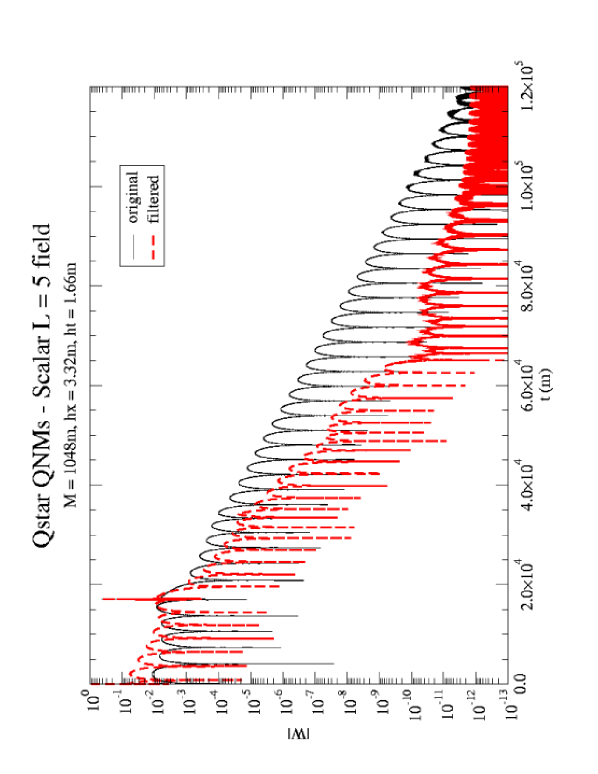
Figure 18: Scalar $\ell=5$ field, $M=1048m$. Notice the first overtone.

In Fig. (17), for example, one has a secondary mode with $\omega=0.00105-0.000400i$, compared to $\omega=0.000706-0.000178i$ for the fundamental mode. For the scalar $\ell=5$ field, in Fig. (18), the figures are $\omega=0.00135-0.000364i$ and $0.00106-0.000206i$, respectively. That is, overtones were a recurrent theme in our quest for stellar modes.

The oscillations become slower as the masses increase, and so does the damping rates, much as in the Schwarzschild BH case, and contrary to the neutron star case.

V Comparative Charts

In this section we compare all kinds of stars mentioned in this paper between themselves and to Schwarzschild BHs.

$Mass$	$Star/BH$	$\ell$	$\omega_{R}$	$-\omega_{I}$
$1048.25$	$NS$	$2$	$3.78E-4$	$2.86E-4$
$1048.25$	$NS$	$3$	$4.86E-4$	$3.15E-4$
$1048.25$	$NS$	$4$	$5.91E-4$	$3.58E-4$
$1048.25$	$NS$	$5$	$7.06E-4$	$3.94E-4$
$1048.25$	$QS$	$1$	$3.47E-4$	$1.45E-4$
$1048.25$	$QS$	$2$	$5.26E-4$	$1.63E-4$
$1048.29$	$QS$	$3$	$7.06E-4$	$1.78E-4$
$1048.29$	$QS$	$4$	$8.85E-4$	$1.92E-4$
$1048.25$	$QS$	$5$	$1.06E-3$	$2.06E-4$
$1048.25$	$SCH$	$3$	$6.4428E-4$	$9.206E-5$
$1048.25$	$SCH$	$4$	$8.2749E-4$	$9.196E-5$
$1048.25$	$SCH$	$5$	$1.0108E-3$	$9.190E-5$
$977.12$	$NS$	$1$	$-$	$-$
$977.12$	$NS$	$2$	$-$	$-$
$977.12$	$NS$	$3$	$4.04E-4$	$3.18E-4$
$977.12$	$NS$	$4$	$4.78E-4$	$3.41E-4$
$977.12$	$NS$	$5$	$5.64E-4$	$3.45E-4$
$977.12$	$QS$	$1$	$3.58E-4$	$1.84E-4$
$977.12$	$QS$	$2$	$5.42E-4$	$2.09E-4$
$977.12$	$QS$	$3$	$7.26E-4$	$2.27E-4$
$977.12$	$QS$	$4$	$9.11E-4$	$2.45E-4$
$977.12$	$QS$	$5$	$1.09E-3$	$2.62E-4$
$977.12$	$SCH$	$1$	$2.9980E-4$	$9.9953E-5$
$977.12$	$SCH$	$2$	$4.9497E-4$	$9.9025E-5$
$977.12$	$SCH$	$3$	$6.9118E-4$	$9.8759E-5$
$977.12$	$SCH$	$4$	$8.8773E-4$	$9.8649E-5$
$977.12$	$SCH$	$5$	$1.0844E-3$	$9.8589E-5$

Table 8: Comparing neutron stars (NS) to quark stars (QS) to Schwarzschild black holes (SCH), scalar field. Fields measured at the stellar surface, for stars.

$846.54$	$NS$	$1$	$-$	$-$
$846.54$	$NS$	$2$	$-$	$-$
$846.54$	$NS$	$3$	$3.55E-4$	$2.79E-4$
$846.54$	$NS$	$4$	$4.05E-4$	$3.28E-4$
$846.54$	$NS$	$5$	$4.86E-4$	$3.31E-4$
$846.54$	$QS$	$1$	$3.76E-4$	$2.38E-4$
$846.54$	$QS$	$2$	$5.77E-4$	$2.90E-4$
$846.54$	$QS$	$3$	$7.75E-4$	$3.04E-4$
$846.54$	$QS$	$4$	$9.79E-4$	$3.13E-4$
$846.54$	$QS$	$5$	$1.17E-3$	$3.58E-4$
$846.54$	$SCH$	$1$	$3.4604E-4$	$1.1537E-4$
$846.54$	$SCH$	$2$	$5.7132E-4$	$1.1430E-4$
$846.54$	$SCH$	$3$	$7.9780E-4$	$1.1399E-4$
$846.54$	$SCH$	$4$	$1.0247E-3$	$1.1387E-4$
$846.54$	$SCH$	$5$	$1.2517E-3$	$1.1380E-4$

Table 9: Continuation of the previous table.

$Mass$	$Star/BH$	$\ell$	$\Omega_{R}$	$-\Omega_{I}$
$1048.25$	$NS$	$2$	$2.81E-4$	$2.49E-4$
$1048.25$	$NS$	$3$	$4.23E-4$	$2.49E-4$
$1048.25$	$NS$	$4$	$5.61E-4$	$3.45E-4$
$1048.25$	$NS$	$5$	$6.65E-4$	$3.44E-4$
$1048.25$	$SCH$	$2$	$3.5647E-4$	$8.4865E-5$
$1048.25$	$SCH$	$3$	$5.7185E-4$	$8.8436E-5$
$1048.25$	$SCH$	$4$	$7.7193E-4$	$8.9829E-5$
$1048.25$	$SCH$	$5$	$9.6570E-4$	$9.0504E-5$
$977.12$	$NS$	$2$	$-$	$-$
$977.12$	$NS$	$3$	$3.25E-4$	$2.46E-4$
$977.12$	$NS$	$4$	$4.42E-4$	$3.25E-4$
$977.12$	$NS$	$5$	$5.70E-4$	$3.84E-4$
$977.12$	$SCH$	$2$	$3.8242E-4$	$9.1043E-5$
$977.12$	$SCH$	$3$	$6.1348E-4$	$9.4874E-5$
$977.12$	$SCH$	$4$	$8.2813E-4$	$9.6368E-5$
$977.12$	$SCH$	$5$	$1.0360E-3$	$9.7093E-4$
$846.54$	$NS$	$2$	$-$	$-$
$846.54$	$NS$	$3$	$-$	$-$
$846.54$	$NS$	$4$	$3.64E-4$	$2.96E-4$
$846.54$	$NS$	$5$	$4.42E-4$	$3.04E-4$
$846.54$	$SCH$	$2$	$4.4141E-4$	$1.0509E-4$
$846.54$	$SCH$	$3$	$7.0811E-4$	$1.0951E-4$
$846.54$	$SCH$	$4$	$9.5587E-4$	$1.1123E-4$
$846.54$	$SCH$	$5$	$1.1958E-3$	$1.1207E-4$

Table 10: Comparing neutron stars (NS) to Schwarzschild black holes (SCH), axial field. Fields measured at the stellar surface, for stars.

We did not place $M\omega$ in tables (8), (9) and (10) because the neutron and quark stars do not share the simple $\omega\propto\frac{1}{M}$ property with the Schwarzschild BHs, as seen in their respective sections. From the aforementioned tables we learn that the neutron stars modes are more strongly damped than its quark counterparts and these are, in turn, more damped than Schwarzschild modes. The Schwarzschild modes oscillate faster than the neutron star modes, but slightly less than the quark star modes.

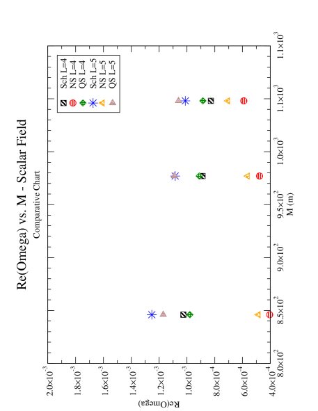
Figure 19: Comparing Frequencies. Real Part. Scalar Field.

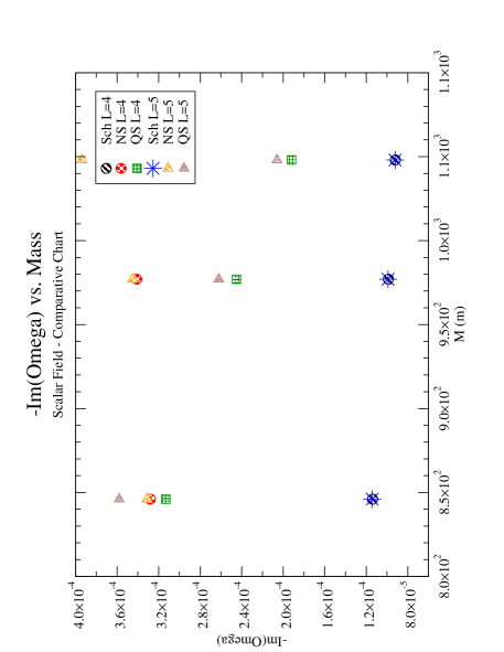
Figure 20: Comparing Frequencies. Imaginary Part. Scalar Field.

VI Final Remarks and Conclusions

First of all, the oscillating frequencies of the QNMs ($\omega_{R}$) increases with increasing $\ell$, for a given mass and perturbation, as in the black-hole case, irrespective of the star type. The damping $-\omega_{I}$ of the modes, however, decreases with increasing $\ell$, and does so very markedly, for all the masses and fields under study for uniform stars, whereas in the Schwarzschild black-hole (SchBH) case $-\omega_{I}$ has a very slight increase instead for the axial field, while also decreasing (very slightly, though) for the scalar field. This is an interesting contrast. And uniform stars showed stronger dampings for axial fields than for scalar fields, also contrary to SchBH.

The neutron stars (NS) and quark stars (QS) modes, in general, showed an increase in $-\omega_{I}$ with increased $\ell$ for scalar perturbations. For the axial modes, a similar trend could be detected for NS, and the only possible anomaly could be the $M=1048m$ case, when the $\ell=4$ mode had practically the same damping ratio as the $\ell=5$ mode, as can be seen at the end of the table (10).

There is also a clear dependence of the modes on the uniform star mass mass, for a given compactness and perturbation, as in the Schwarzschild case: the more massive a uniform star is, the slower is the oscillation of the field and the weaker is its damping. The same holds for the overtones we have found for them. As for the compactness $c$ itself, given a fixed mass, an increase in $c$ made both $Re(\omega)$ and $-Im(\omega)$ decrease, that is, more compact stars had slower and (much) less damped oscillations.

The case of competing modes (overtones) in stars needed our foremost attention, since it seems not to have been mentioned anywhere so far. We could detect such competing modes in very compact uniform stars, especially when $c\thickapprox 0.77$ onwards. And here comes another contrast: while in the Schwarzschild black hole context the overtones have oscillated more slowly than the fundamental mode (see Konoplya03 , dgiugno-06 ), for the uniform stars the opposite was true. A similar feature was detected for some QS modes in which the presence of overtones was detectable, although we could not find clear overtones for NS.

In general, leaving aside the uniform stars (UniS) due to their dependency on $c$, given some perturbation type, $M$ and $\ell$, QS modes tend to oscillate a bit faster than SchBH modes for higher masses and slightly slower for smaller masses, and these, in turn, oscillate faster than NS modes. When it comes to damping, though, the Sch BH modes are the least damped of all, followed by the QS modes (at least twice as damped) and by NS modes (the most damped of all). That is, NS modes are the slowest in oscillation rate and the most damped. At least, in the mass range under scrutiny.

Nevertheless, if UniS are considered, their modes have slightly higher $\omega_{R}$ than SchBHs, but their $-\omega_{I}$ can be much smaller than their Sch BH counterparts, so that these uniform stellar modes are, in fact, the LEAST damped of all modes, particularly when $c$ increases towards its limiting value of $8/9$.

The Sch BH and the uniform stars have a simple scaling property for $\omega$, namely $M\omega=k$, where $k$ is a constant depending on the perturbation, on $\ell$ and, for the uniform stars, $c$. Not so for the NS and QS modes, where we have not found so simple a correlation between $M$ and $\omega$. For QS at least, a decreasing $M$ meant an increasing $\omega$ (especially for $\omega_{R}$). For NS, a curious feature emerged: the larger $M$ is, the higher $\omega$ is, especially $\omega_{R}$, in sharp contrast to what has been seen for SchBH, UniS and QS. At any rate, however, in the mass range we have worked with, even the most massive NS have presented modes which were slower and more damped than the most massive SchBH, UniS and QS modes. We are still in the search for the reason(s) for such a behaviour.

Appendix A Brief Theory of Uniform Stars

Uniform stars are stars possessing a uniform density $\varepsilon_{0}$, and references abound in the literature, as in Weinberg . For these stars, computations are very easy, as we shall see.

The star mass function is simply

$$m(r)=4\pi\frac{\varepsilon_{0}r^{3}}{3},$$ (5)

if $r\leq R$ and $m(r)=M$ if $r>R$. Hence, in terms of the radius $R$ and the mass $M$ of the star, one has $\varepsilon_{0}=\frac{3M}{4\pi R^{3}}$.

The pressure is determined via the Oppenheimer-Volkov equation,

$$\frac{dp}{dr}=-\frac{(p+\varepsilon)(m+4\pi r^{3}p)}{r^{2}(1-\frac{2m}{r})},$$ (6)

and is given by

$$p(r)=\frac{3M}{4\pi R^{3}}[\frac{\sqrt{1-\frac{2M}{R}}-\sqrt{1-\frac{2Mr^{2}}{R^{3}}}}{\sqrt{1-\frac{2Mr^{2}}{R^{3}}}-3\sqrt{1-\frac{2M}{R}}}],$$ (7)

which approaches zero smoothly as $r\to R$. The $g_{tt}$ term of the metric is given by

$$g_{tt}=-\frac{1}{4}(3\sqrt{1-\frac{2M}{R}}-\sqrt{1-\frac{2Mr^{2}}{R^{3}}})^{2},$$ (8)

which reduces to the Schwarzschild $g_{tt}$ for $r>R$. One point is of utmost importance in what follows: the expression for $p$ becomes singular when $M/R>4/9$. Since the star pressure cannot be infinite anywhere, one concludes that there is an upper limit to the degree of compactness ($c=2M/R$) for any star. In fact, since $M/R$ cannot exceed $4/9$, no star can have $c>8/9$, so there’s a gap in $c$ between Schwarzschild black holes and spherically symmetric stars of any kind. This limitation stems from General Relativity itself, not from any particular stellar model.

From the existing literature Chand-Ferr ,Chand-FerrB we have the wave equation satisfied by the scalar and gravitational perturbations, namely

$$\frac{\partial^{2}W}{\partial x^{2}}-\frac{\partial^{2}W}{\partial t^{2}}=VW,$$ (9)

where $W$ stands for the perturbation amplitude and $V$, the perturbative potential. The latter is written as

$$V = \frac{1}{4}(3\sqrt{1-\frac{2M}{R}}-\sqrt{1-\frac{2Mr^{2}}{R^{3}}})^{2}[\frac{\ell(\ell+1)}{r^{2}}+\frac{2\sigma m(r)}{r^{3}}+4\pi(\varepsilon_{0}-p(r))]$$

$$V = (1-\frac{2M}{r})[\frac{\ell(\ell+1)}{r^{2}}+\frac{2\sigma M}{r^{3}}],$$ (10)

where $\sigma=1,0,-3$ depending on whether we are dealing with scalar, electromagnetic or axial perturbations. The first of these equations holds inside the star, and the latter holds outside.

We can now illustrate some of the potentials, and find out how they change with the compactness. Such an illustration is available in Fig. (21).

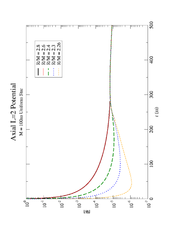
Figure 21: Graph of de $V$ vs. $r$ for a compact star. Axial $\ell=2$ case shown.

Appendix B The Numerical Method

We have employed a direct numerical method consisting of a grid in the tortise coordinate $x$ and the time coordinate $t$. Since $x$ runs from some finite $x_{0}$ at $r=0$ to $x\to\infty$ when $r\to\infty$, we start by specifying the field $W$ (scalar or axial) and its time derivative at $t=0$ in the region of interest in $x$ (usually a Gaussian wave packet centered around some $x_{1}>x_{0}$). The time evolution of the field is given by

$$\Psi(t_{0}+\delta t,x_{0}) = -\Psi(t_{0}-\delta t,x_{0})+(2-\delta^{2}xV(x_{0})-\frac{5\delta t^{2}}{2\delta x^{2}})\Psi(t_{0},x_{0})+$$ (11)

$$+ \frac{4\delta t^{2}[\Psi(t_{0},x_{0}+\delta x)+\Psi(t_{0},x_{0}-\delta x)]}{3\delta x^{2}}-$$

$$- \frac{\delta t^{2}[\Psi(t_{0},x_{0}-2\delta x)+\Psi(t_{0},x_{0}+2\delta x)]}{12\delta x^{2}},$$

in which $\delta x$ is the spacing in $x$ and $\delta t$ is the time step. Given the ratio $m=\frac{\delta t}{\delta x}$ (the so-called mesh ratio), one must have $m<1$ for the sake of convergence. We stop at some $t>t_{0}$ and analyse the data for all $x$ at that time. Reflection may occur at the borders of the grid.

References

- (1) Chandrasekhar, S. and Ferrari, V., Proc. R. Soc. Lond. A434 (1991) 449-457.
- (2) Chandrasekhar, S. and Ferrari, V., Proc. R. Soc. Lond.A 434 (1991) 247-279.
- (3) Kokkotas, K. D. and Schmidt, B. G., Living Relativity Review 2, 2(1999); Bin Wang Braz. J. Phys. 35 (2005) 1029, gr-qc/0511133.
- (4) Price, R. H., Phys. Rev. D5, 2419 (1972) and Phys. Rev. D5, 2439 (1972).
- (5) Wang, B., Molina, C. and Abdalla, E., Phys. Rev. D63, 084001 (2001).
- (6) Wang, B., Lin, C. and Abdalla, E., Phys. Lett. B481, 79 (2000).
- (7) Abdalla, E., Castello-Branco, K. H. C. and Lima-Santos, A., Phys. Rev. D66 104018 (2002).
- (8) Oppenheimer, J. R. and Volkov, G. M., Phys. Rev. 55, 374 (1939).
- (9) Weinberg, S. Gravitation and Cosmology, John Wiley and Sons (1972).
- (10) Haensel, P. Final Stages of Stellar Evolution, EAS Publication Series 7, 249-282 (2003).
- (11) Witten, E. Phys. Rev. D 30, 272 (1984).
- (12) Molina, C., Giugno, D., Abdalla, E. and Saa, A., Phys. Rev. D69, 104013 (2004).
- (13) R. A. Konoplya, Journal of Physical Studies 8 (2004) 93-100.
- (14) Abdalla, E. and Giugno, D., gr-qc/0611023.
- (15) Weber, F., Strange Quark Matter and Compact Stars, astro-ph/0407155.
- (16) Glendenning, N. K., Compact Stars - Nuclear Physics, Particle Physics and General Relativity, Second Edition, AA Library, Springer, 2000.
- (17) Zhang, Y. and Su, R.-K., Phys. Rev. C67, 015202 (2003).