Conditions for the cosmological viability of $f(R)$ dark energy models

Abstract

We derive the conditions under which dark energy models whose Lagrangian densities $f$ are written in terms of the Ricci scalar $R$ are cosmologically viable. We show that the cosmological behavior of $f(R)$ models can be understood by a geometrical approach consisting in studying the $m(r)$ curve on the $(r,m)$ plane, where $m\equiv Rf_{,RR}/f_{,R}$ and $r\equiv-Rf_{,R}/f$ with $f_{,R}\equiv{\rm d}f/{\rm d}R$. This allows us to classify the $f(R)$ models into four general classes, depending on the existence of a standard matter epoch and on the final accelerated stage. The existence of a viable matter dominated epoch prior to a late-time acceleration requires that the variable $m$ satisfies the conditions $m(r)\approx+0$ and ${\rm d}m/{\rm d}r>-1$ at $r\approx-1$. For the existence of a viable late-time acceleration we require instead either (i) $m=-r-1$ , $(\sqrt{3}-1)/2<m\leq 1$ and ${\rm d}m/{\rm d}r<-1$ or (ii) $0\leq m\leq 1$ at $r=-2$. These conditions identify two regions in the $(r,m)$ space, one for the matter era and the other for the acceleration. Only models with a $m(r)$ curve that connects these regions and satisfy the requirements above lead to an acceptable cosmology. The models of the type $f(R)=\alpha R^{-n}$ and $f=R+\alpha R^{-n}$ do not satisfy these conditions for any $n>0$ and $n<-1$ and are thus cosmologically unacceptable. Similar conclusions can be reached for many other examples discussed in the text. In most cases the standard matter era is replaced by a cosmic expansion with scale factor $a\propto t^{1/2}$. We also find that $f(R)$ models can have a strongly phantom attractor but in this case there is no acceptable matter era.

I Introduction

The late-time accelerated expansion of the universe is a major challenge to present-day cosmology (see Refs. review ; CST for review). A consistent picture, the concordance model, seems to emerge from the bulk of observations probing the background evolution of the universe as well as its inhomogeneities: Supernovae Ia SN , Cosmic Microwave Background anisotropies (CMB) CMB , Large Scale Structure formation (LSS) LSS , baryon oscillations BAO , weak lensing WL , etc. If one assumes today a flat universe with a cosmological constant $\Lambda$ and with pressureless matter, observations suggest the following cosmological parameters $\Omega_{\Lambda,0}\approx 0.7$, $\Omega_{{\rm m},0}\approx 0.3$ where $\Omega_{X,0}=\rho_{X,0}/\rho_{{\rm cr},0}$ for any component $X$, where the subscript $0$ stands for present-day values and $\rho_{{\rm cr}}$ is the critical density of the universe.

A cosmological constant term is the simplest possibility to explain the observational data. In fact the recent data analysis Sel combining the SNLS data Astier with CMB, LSS and the Lyman-$\alpha$ forest shows that, assuming $w_{{\rm DE}}$ is constant the equation of state parameter of Dark Energy (DE) is found to be $w_{{\rm DE}}=-1.04\pm 0.06$ and therefore consistent with a cosmological constant. However a cosmological constant suffers from an extreme fine-tuning problem of its energy scale if it originates from vacuum energy. For this reason several works have explored alternative explanations, i.e., dynamical forms of dark energy. In the absence of any compelling dynamical dark energy model, further insight can be gained by considering general models with constant equation of state or some fiducial parametrization, see e.g. CP01 , and SS06 for a recent review.

The first alternative possibility to a cosmological constant is a minimally coupled scalar field $\phi$, usually called quintessence quin . In analogy with inflationary scenarios, this scalar field would be responsible for a stage of accelerated expansion while in contrast to inflation this stage occurs in the late-time evolution of the universe. The energy density of the scalar field should therefore come to dominate over other components in the universe only recently. This is the so called cosmic coincidence problem faced by most dark energy models. In order to alleviate this problem various generalizations have been considered, like coupled quintessence models coupled in which matter and dark energy scale in the same way with time during some epochs. It is however still a challenging task to construct viable scaling models which give rise to a matter-dominated era followed by an accelerated scaling attractor AQTW .

An important limitation of standard quintessence models is that they do not allow for a phantom regime with $w_{{\rm DE}}<-1$. A phantom regime is allowed by observations and even favored by some analysis of the data Mel . To achieve $w_{{\rm DE}}<-1$, the scalar field should be endowed with a generalized kinetic term, for instance one with a sign opposite to the canonical one phantom . This intriguing possibility is however plagued by quantum instabilities Cline . A further interesting possibility is provided by non-minimally coupled scalar fields nonmin and scalar-tensor cosmology stensor ; Esp . Scalar-tensor DE models can have a consistent phantom regime and a modified growth rate of structure BEPS00 , see also GPRS06 for a systematic study of the low redshift structure of such theories including a detailed analysis of the possibility to have a phantom regime and the constraints from local gravity tests, and Peri for some concrete examples of this scenario. In scalar-tensor DE models gravity is modified by an additional dynamical degree of freedom, the scalar partner of the graviton.

Recently there has been a burst of activity dealing with so-called modified gravity DE models (see Ref. CST for recent review and references therein). In these theories one modifies the laws of gravity whereby a late-time accelerated expansion is produced without recourse to a DE component, a fact which renders these models very attractive. In some models one can have in addition a phantom regime, which might constitute an interesting feature.

The simplest family of modified gravity DE models is obtained by replacing the Ricci scalar $R$ in the usual Hilbert-Einstein Lagrangian density for some function $f(R)$. In the first models proposed in DE literature, where a term $1/R$ is added to $R$ Capo ; Carroll , one typically expects that as the universe expands the inverse curvature term will dominate and produce the desired late-time accelerated expansion (see Ref. coa for a pioneering work in the context of inflation). However it was quickly realized that local gravity constraints would make these models non viable Chiba (see also Ref. Dolgov ). Indeed, it was shown that $f(R)$ models are formally equivalent to scalar-tensor models with a vanishing Brans-Dicke parameter $\omega_{{\rm BD}}=0$. Clearly such models do not pass local gravity (solar system) constraints, in particular the post Newtonian parameter $\gamma_{{\rm PPN}}$ satisfies $\gamma_{{\rm PPN}}=1/2$ instead of being very close to 1 as required by observations.

However, the question of whether local gravity constraints rule out or not $f(R)$ models does not seem to be completely settled in the literature Faraoni . Several papers pointed out that local gravity constraints cannot yet rule out all possible forms of $f(R)$ theories. For instance, a model containing a particular combination of $1/R$ and $R^{2}$ terms was suggested NO03 and claimed by their authors to pass successfully the solar system constraints, due to a large (infinite) effective mass needed to satisfy solar system constraints, and also to produce a late-time accelerated expansion (though this latter property does not seem to have been demonstrated in a satisfactory way). Another original approach with negative and positive power terms was suggested recently where the positive power term would dominate on small scales while the negative power term dominates on large cosmic scales thereby producing the accelerated expansion Brook (see however nva ). See Refs. fRpapers for a list of recent research in $f(R)$ dark energy models. If $f(R)$ models are not ruled out by local gravity constraints it is important to understand their cosmological properties.

Recently three of the present authors APT have shown that the large redshift behavior of $f(R)=R+\alpha R^{-n}$ models generically lead to the “wrong” expansion law: indeed, the usual matter era preceding the late-time accelerated stage does not have the usual $a\propto t^{2/3}$ behavior but rather $a\propto t^{1/2}$ which would obviously make these models cosmologically unacceptable. This intriguing and quite unexpected property of these $f(R)$ models was overlooked in the literature. The absence of the standard matter epoch is associated with the fact that in the Einstein frame non-relativistic matter is strongly coupled to gravity except for the $f(R)$ theories which have a linear dependence of $R$ (including the $\Lambda$CDM model: $f(R)=R-\Lambda)$ APT .

In the Einstein frame the power-law models $f(R)\propto R^{-n}$ ($n\neq-1$) correspond to a coupled quintessence scenario with an exponential potential of a dynamical scalar field. In this case the standard matter era is replaced by a “$\phi$ matter-dominated epoch” ($\phi$MDE) in which the scale factor in the Einstein frame evolves as $a_{E}\propto t_{E}^{3/5}$ APT . Transforming back to the Jordan frame, this corresponds to a non-standard evolution $a\propto t^{1/2}$. We wish to stress here that cosmological dynamics obtained in the Jordan frame exhibits no difference from the one which is transformed to the Einstein frame and transformed back to the original frame. Hence in this paper we shall focus on the analysis in the Jordan frame without referring to the Einstein frame.

This paper is devoted to explaining in detail our previous result and, more importantly, to extend it to all well-behaved $f(R)$ Lagrangians. Despite almost thirty years of work on the cosmology of $f(R)$ models, there are in fact no general criteria in literature to gauge their validity as alternative cosmological models (see Ref. key-2 for one of the earliest attempt in this direction). We find the general conditions for a $f(R)$ theory to contain a standard matter era followed by an accelerated attractor in a spatially flat, homogeneous and isotropic background. The only conditions we assume throughout this paper, beside obviously a well-behaved function $f(R)$ continuous with all its derivatives, is that ${\rm d}f/{\rm d}R>0$, to maintain a positive effective gravitational constant in the limit of vanishing higher-order term. In some cases however we consider $f(R)$ models which violate this condition in some range of $R$, but not on the actual cosmological trajectories. The main result of this paper is that we are able to show analytically and numerically that all $f(R)$ models with an accelerated global attractor belong to one of four classes:

• Class I : Models of this class possess a peculiar scale factor behavior ($a\propto t^{1/2}$) just before the acceleration.

• Class II : Models of this class have a matter epoch and are asymptotically equivalent to (and hardly distinguishable from) the $\Lambda$CDM model ($w_{{\rm eff}}=-1$).

• Class III : Models of this class can possess an approximate matter era but this is a transient state which is rapidly followed by the final attractor. Technically, the eigenvalues of the matter saddle point diverge and is very difficult to find initial conditions that display the approximated matter epoch.

• Class IV : Models of this class behave in an acceptable way. They possess an approximate standard matter epoch followed by a non-phantom acceleration ($w_{{\rm eff}}>-1$).

We can then summarize our findings by saying that $f(R)$ dark energy models are either wrong (Class I), or asymptotically de-Sitter (Class II), or strongly phantom (Class III) or, finally, standard DE (Class IV). The second and fourth classes have some chance to be cosmologically acceptable, but even for these cases it is not an easy task to identify the basin of attraction of the acceptable trajectories. We fully specify the conditions under which any given $f(R)$ model belongs to one of the classes above and discuss analytically and numerically several examples belonging to all classes.

An important clarification is here in order. It is clear that $f(R)$ gravity models can be perfectly viable in different contexts. The most famous example is provided by Starobinsky’s model, $f(R)=R+\alpha R^{2}$ star , which has been the first internally consistent inflationary model. In this model, the $R^{2}$ term produces an accelerated stage in the early universe preceding the usual radiation and matter stages. A late-time acceleration in this model (after the matter dominated stage) requires a positive cosmological constant (or some other form of dark energy) in which case the $R^{2}$ term is no longer responsible for the late-time acceleration.

Our paper is organized in the following way. Section II contains the basic equations in the Jordan frame and introduces autonomous equations which are applicable to any forms of $f(R)$. In Sec. III we derive fixed points together with their stabilities and present the conditions for viable $f(R)$ DE models. In Sec. VI we classify $f(R)$ DE models into four classes depending upon the cosmological evolution which gives the late-time acceleration. In Sec. V we shall analytically show the cosmological viability for some of the $f(R)$ models by using the conditions found in Sec. III. Section VI is devoted to a numerical analysis for a number of $f(R)$ models to confirm the analytical results presented in the previous section. Finally we summarize our results in Section VII. We will always work in the Jordan frame, in order to show the properties of $f(R)$ models in the most direct way, without the need to convert back from the Einstein frame.

II $f(R)$ dark energy models

II.1 Definitions and equations

In this section we derive all basic equations in the Jordan frame (JF), the frame in which observations are performed. We will further define all fundamental quantities characterizing our system, in particular the equation of state of our system. Actually, as we will see below this is a subtle issue and we have to define what is meant by the Dark Energy (DE) equation of state.

We concentrate on spatially flat Friedman-Lemaître-Robertson-Walker (FLRW) universes with a time-dependent scale factor $a(t)$ and a metric

$${\rm d}s^{2}=-{\rm d}t^{2}+a^{2}(t)\,{\rm d}{\bf x}^{2}\,.$$ (1)

For this metric the Ricci scalar $R$ is given by

$$R=6\left(2H^{2}+\dot{H}\right)\,,$$ (2)

where $H\equiv\dot{a}/a$ is the Hubble rate and a dot stands for a derivative with respect to $t$.

We start with the following action in the JF

$$S=\int{\rm d}^{4}x\sqrt{-g}\left[\frac{1}{2\kappa^{2}}f(R)+{\mathcal{L}}_{{\rm rad}}+{\mathcal{L}}_{{\rm m}}\right]\,,$$ (3)

where $\kappa^{2}=8\pi G$ while $G$ is a bare gravitational constant, $f(R)$ is some arbitrary function of the Ricci scalar $R$, and ${\mathcal{L}}_{{\rm m}}$ and ${\mathcal{L}}_{{\rm rad}}$ are the Lagrangian densities of dust-like matter and radiation respectively. Note that $G$ is typically not Newton’s gravitational constant measured in the attraction between two test masses in Cavendish-type experiments (see e.g. Esp ). Then the following equations are obtained Jaichan

$$3FH^{2} = \kappa^{2}\,(\rho_{{\rm m}}+\rho_{{\rm rad}})+\frac{1}{2}(FR-f)-3H\dot{F}\,,$$ (4)

$$-2F\dot{H} = \kappa^{2}\left(\rho_{{\rm m}}+\frac{4}{3}\rho_{{\rm rad}}\right)+\ddot{F}-H\dot{F}\,,$$ (5)

where

$$F\equiv\frac{{\rm d}f}{{\rm d}R}\,.$$ (6)

In standard Einstein gravity ($f=R$) one has $F=1$. In what follows we shall consider the positive-definite forms of $F$ to avoid a singularity at $F=0$. The densities $\rho_{{\rm m}}$ and $\rho_{{\rm rad}}$ satisfy the usual conservation equations

$$\dot{\rho}_{{\rm m}}+3H\rho_{{\rm m}}=0\,,$$ (7)

$$\dot{\rho}_{{\rm rad}}+4H\rho_{{\rm rad}}=0\,.$$ (8)

We note that Eqs. (4) and (5) are similar to those obtained for scalar-tensor gravity BEPS00 with a vanishing Brans-Dicke parameter $\omega_{{\rm BD}}=0$ and a specific potential $U=(FR-f)/2$. Note that in scalar-tensor gravity we have $FR=L$ so that this term vanishes, while Eq. (5) is similar except for the fact that a kinematic term of the scalar field is absent. Hence we can define the DE equation of state in a way similar to that in scalar-tensor theories of gravity (see e.g., GPRS06 ; T02 ). With a straightforward redefinition of the quantities, we rewrite Eqs. (4) and (5) as follows

$$3F_{0}H^{2} = \kappa^{2}(\rho_{{\rm DE}}+\rho_{{\rm m}}+\rho_{{\rm rad}})\,,$$ (9)

$$-2F_{0}\dot{H} = \kappa^{2}\left(\rho_{{\rm m}}+\frac{4}{3}\rho_{{\rm rad}}+\rho_{{\rm DE}}+p_{{\rm DE}}\right)\,.$$ (10)

We then have the following equalities

$$\kappa^{2}\,\rho_{{\rm DE}} = \frac{1}{2}(FR-f)-3H\dot{F}+3H^{2}(F_{0}-F)\,,$$ (11)

$$\kappa^{2}\,p_{{\rm DE}} = \ddot{F}+2H\dot{F}-\frac{1}{2}(FR-f)-(2\dot{H}+3H^{2})(F_{0}-F)\,.$$ (12)

The energy density $\rho_{{\rm DE}}$ and the pressure density $p_{{\rm DE}}$ of DE defined in this way satisfy the usual conservation equation

$${\dot{\rho}_{{\rm DE}}}=-3H(\rho_{{\rm DE}}+p_{{\rm DE}})\,.$$ (13)

Hence the equation of state parameter $w_{{\rm DE}}$ defined through

$$w_{{\rm DE}}\equiv\frac{p_{{\rm DE}}}{\rho_{{\rm DE}}}=-1+\frac{2\ddot{F}-2H\dot{F}-4\dot{H}(F_{0}-F)}{(FR-f)-6H\dot{F}+6H^{2}(F_{0}-F)}\,,$$ (14)

acquires its usual physical meaning, in particular the time evolution of the DE sector is given by

$$\frac{\rho_{{\rm DE}}(z)}{\rho_{{\rm DE,0}}}=\exp\left[3\int_{0}^{z}{\rm d}z^{\prime}\leavevmode\nobreak\ \frac{1+w_{{\rm DE}}(z^{\prime})}{1+z^{\prime}}\right]\,,$$ (15)

where $z\equiv a_{0}/a-1$. Note that the subscript “0” stands for present values. It is $\rho_{{\rm DE}}$, as defined in Eq. (11) which is the quantity extracted from the observations and $w_{{\rm DE}}$ the corresponding DE equation of state parameter for which specific parametrizations are used.

Looking at Eqs. (9) and (LABEL:E20), one could introduce the cosmological parameters $\tilde{\Omega}_{X}=\kappa^{2}\rho_{X}/(3F_{0}H^{2})$ GPRS06 ; T02 . However here it turns out to be more convenient to work with the density parameters

$$\Omega_{X}\equiv\leavevmode\nobreak\ \frac{\kappa^{2}\rho_{X}}{3FH^{2}}\,,$$ (16)

where $X={\rm m},{\rm rad}$ or ${\rm DE}$. The quantity $w_{{\rm DE}}$ can further be obtained directly from the observations

$$w_{{\rm{DE}}} = \frac{(1+z)\,{\rm d}h^{2}/{\rm d}z-3h^{2}-\Omega_{{\rm rad,0}}(1+z)^{4}}{3[h^{2}-\Omega_{{\rm m},0}(1+z)^{3}-\Omega_{{\rm rad},0}(1+z)^{4}]}\,,$$ (17)

where $h\equiv H/H_{0}$. In the low-redshift region where the contribution of the radiation is negligible, we have

$$w_{{\rm{DE}}} = \frac{(1+z)\,{\rm d}h^{2}/{\rm d}z-3h^{2}}{3[h^{2}-\Omega_{{\rm m},0}(1+z)^{3}]}\,,\qquad z\ll z_{{\rm eq}}\,,$$ (18)

where $z_{{\rm eq}}$ is the redshift at which dust and radiation have equal energy densities. Equation (17) can be extended for spatially non-flat universes PR05 but we restrict ourselves to spatially flat universes. We also define the effective equation of state

$$w_{{\rm eff}}=-1-\frac{2\dot{H}}{3H^{2}}\,.$$ (19)

Note that the following equality holds

$$w_{{\rm eff}}=\tilde{\Omega}_{{\rm DE}}\leavevmode\nobreak\ w_{{\rm DE}}+\frac{1}{3}\tilde{\Omega}_{{\rm rad}}\,,$$ (20)

if we define $\tilde{\Omega}_{X}=\kappa^{2}\rho_{X}/(3F_{0}H^{2})$.

II.2 Autonomous equations

For a general $f(R)$ model it will be convenient to introduce the following (dimensionless) variables

$$x_{1} = -\frac{\dot{F}}{HF}\,,$$ (21)

$$x_{2} = -\frac{f}{6FH^{2}}\,,$$ (22)

$$x_{3} = \frac{R}{6H^{2}}=\frac{\dot{H}}{H^{2}}+2\,,$$ (23)

$$x_{4} = \leavevmode\nobreak\ \frac{\kappa^{2}\rho_{{\rm rad}}}{3FH^{2}}\,.$$ (24)

From Eq. (4) we have the algebraic identity

$$\Omega_{{\rm m}}\equiv\frac{\kappa^{2}\rho_{{\rm m}}}{3FH^{2}}=1-x_{1}-x_{2}-x_{3}-x_{4}\,.$$ (25)

It is then straightforward to obtain the following equations of motion

$$\frac{{\rm d}x_{1}}{{\rm d}N} = -1-x_{3}-3x_{2}+x_{1}^{2}-x_{1}x_{3}+x_{4}\leavevmode\nobreak\ ,$$ (26)

$$\frac{{\rm d}x_{2}}{{\rm d}N} = \frac{x_{1}x_{3}}{m}-x_{2}(2x_{3}-4-x_{1})\leavevmode\nobreak\ ,$$ (27)

$$\frac{{\rm d}x_{3}}{{\rm d}N} = -\frac{x_{1}x_{3}}{m}-2x_{3}(x_{3}-2)\leavevmode\nobreak\ ,$$ (28)

$$\frac{{\rm d}x_{4}}{{\rm d}N} = -2x_{3}x_{4}+x_{1}\,x_{4}\,,$$ (29)

where $N$ stands for $\ln a$ and

$$m \equiv \frac{{\rm d}\log F}{{\rm d}\log R}=\frac{Rf_{,RR}}{f_{,R}}\,,$$ (30)

$$r \equiv -\frac{{\rm d}\log f}{{\rm d}\log R}=-\frac{Rf_{,R}}{f}=\frac{x_{3}}{x_{2}}\,,$$ (31)

where $f_{,R}\equiv{\rm d}f/{\rm d}R$ and $f_{,RR}\equiv{\rm d}^{2}f/{\rm d}R^{2}$. Deriving $R$ as a function of $x_{3}/x_{2}$ from Eq. (31), one can express $m$ as a function of $x_{3}/x_{2}$ and obtain the function $m(r)$. For the power-law model with $f(R)=\alpha R^{-n}$ the variable $m$ is a constant ($m=-n-1$) with $r=n=x_{3}/x_{2}$. In this case the system reduces to a 3-dimensional one with variables $x_{1}$, $x_{2}$ and $x_{4}$. However for general $f(R)$ gravity models the variable $m$ depends upon $r$.

We also make use of these expressions:

$$w_{{\rm eff}} = -\frac{1}{3}(2x_{3}-1)\,,$$ (32)

$$w_{{\rm DE}} = \frac{1}{3}\frac{1-x_{4}y-2x_{3}}{1-y(1-x_{1}-x_{2}-x_{3})}\,,$$ (33)

where $y=F/F_{0}$.

III Cosmological dynamics of $f(R)$ gravity models

In this section we derive the analytical properties of the phase space.

III.1 Critical points and stability for a general $f(R)$

In the absence of radiation ($x_{4}=0$) the critical points for the system (26)-(28) for any $m(r)$ are

$$P_{1}:(x_{1},x_{2},x_{3})=(0,-1,2),\quad\Omega_{{\rm m}}=0,\quad w_{{\rm eff}}=-1\,,$$ (34)

$$P_{2}:(x_{1},x_{2},x_{3})=(-1,0,0),\quad\Omega_{{\rm m}}=2,\quad w_{{\rm eff}}=1/3\,,$$ (35)

$$P_{3}:(x_{1},x_{2},x_{3})=(1,0,0),\quad\Omega_{{\rm m}}=0,\quad w_{{\rm eff}}=1/3\,,$$ (36)

$$P_{4}:(x_{1},x_{2},x_{3})=(-4,5,0),\quad\Omega_{{\rm m}}=0,\quad w_{{\rm eff}}=1/3\,,$$ (37)

$$P_{5}:(x_{1},x_{2},x_{3})=\left(\frac{3m}{1+m},-\frac{1+4m}{2(1+m)^{2}},\frac{1+4m}{2(1+m)}\right),\quad\Omega_{{\rm m}}=1-\frac{m(7+10m)}{2(1+m)^{2}},\quad w_{{\rm eff}}=-\frac{m}{1+m}\,,$$ (38)

$$P_{6}:(x_{1},x_{2},x_{3})=\left(\frac{2(1-m)}{1+2m},\frac{1-4m}{m(1+2m)},-\frac{(1-4m)(1+m)}{m(1+2m)}\right),\quad\Omega_{{\rm m}}=0,\quad w_{{\rm eff}}=\frac{2-5m-6m^{2}}{3m(1+2m)}\,,$$ (39)

where here $\Omega_{{\rm m}}=1-x_{1}-x_{2}-x_{3}$.

The points $P_{5}$ and $P_{6}$ satisfy the equation $x_{3}=-(m(r)+1)x_{2}$, i.e.,

$$m(r)=-r-1\,.$$ (40)

When $m(r)$ is not a constant, one must solve this equation. For each root $r_{i}$ one gets a point of type $P_{5}$ or $P_{6}$ with $m=m(r_{i})$. For instance, the $f(R)=R+\alpha R^{-n}$ model corresponds to $m(r)=-n(1+r)/r$ as we will see later, which then gives $r_{1,2}=-1,n$ and $m_{1,2}=0,-1-n$. If we assume that $m={\rm constant}$ then the condition $x_{3}=-(m+1)x_{2}$ must hold from Eqs. (30) and (31). Hence for $m={\rm constant}$ the points $P_{2,3,5,6}$ always exist, while $P_{1}$ and $P_{4}$ are present for $m=1$ and $m=-1$ respectively. The solutions which give the exact equation of state of a matter era ($w_{{\rm eff}}=0$, i.e., $a\propto t^{2/3}$ or $x_{3}=1/2$) exist only for $m=0$ ($P_{5}$) or for $m=-(5\pm\sqrt{73})/12$ ($P_{6}$) Capo06 . However the latter case corresponds to $\Omega_{{\rm m}}=0$, so this does not give a standard matter era dominated by a non-relativistic fluid APT2 .

If $m(r)$ is not constant then there can be any number of distinct solutions, although only $P_{1}$ and those originating from $P_{5,6}$ can be accelerated and only $P_{2}$ and $P_{5}$ might give rise to matter eras. However $P_{2}$ corresponds to $w_{{\rm eff}}=1/3$ and therefore is ruled out as a correct matter era: this is in fact the $a\propto t^{1/2}$ behavior discussed in Ref. APT (and denoted as $\phi$MDE since it is in fact a field-matter dominated epoch in the Einstein frame). On the contrary, $P_{5}$ resembles a standard matter era, but only for $m$ close to 0. Hence a “good” cosmology would be given by any trajectory passing near $P_{5}$ with $m$ close to 0 and landing on an accelerated attractor. Any other behavior would not be consistent with observations.

It is important to realize that the surface $x_{2},x_{3}$ for which $m(r)=-r-1$ is a subspace of the system (26-29) and therefore it cannot be crossed. This can be seen by using the definition of $r$ and $m$ to derive the following equation for $r$:

$$\frac{{\rm d}r}{{\rm d}N}=r(1+m+r)\frac{\dot{R}}{HR}\,,$$ (41)

which shows explicitly that $m=-r-1$ implies ${\rm d}r/{\rm d}N=0$ as long as $\dot{R}/HR$ does not diverge. This means that the evolution of the system along the $m(r)$ line stops at the roots of the equation $m=-r-1$ so that every cosmological trajectory is trapped between successive roots.

In what follows we shall consider the properties of each fixed point in turn. We define $m_{i}\equiv m(P_{i})$ and will always assume a general $m=m(r)$.

• (1) $P_{1}$: de-Sitter point

  Since $w_{{\rm eff}}=-1$ the point $P_{1}$ corresponds to de-Sitter solutions ($\dot{H}=0$) and has eigenvalues

  $$-3,\leavevmode\nobreak\ \leavevmode\nobreak\ \leavevmode\nobreak\ -\frac{3}{2}\pm\frac{\sqrt{25-16/m_{1}}}{2}\,,$$ (42)

  where $m_{1}=m(r=-2)$. Hence $P_{1}$ is stable when $0<m_{1}\leq 1$ and a saddle point otherwise. Then the condition for the stability of the de-Sitter point is given by

  $$0\leq m(r=-2)\leq 1\,.$$ (43)

• (2) $P_{2}$: $\phi$MDE

  Point $P_{2}$ is characterized by a “kinetic” epoch in which matter and field co-exist with constant energy fractions. We denote it as a $\phi$-matter dominated epoch ($\phi$MDE) following Ref. coupled . The eigenvalues are given by

  $$-2,\leavevmode\nobreak\ \leavevmode\nobreak\ \frac{1}{2}\left[7+\frac{1}{m_{2}}-\frac{m_{2}^{\prime}}{m_{2}^{2}}r(1+r)\pm\sqrt{\left\{7+\frac{1}{m_{2}}-\frac{m_{2}^{\prime}}{m_{2}^{2}}r(1+r)\right\}^{2}-4\left\{12+\frac{3}{m_{2}}-\frac{m_{2}^{\prime}}{m_{2}^{2}}r(3+4r)\right\}}\right]\,,$$ (44)

  where a prime represents a derivative with respect to $r$. Hence $P_{2}$ is either a saddle or a stable node. If $m(r)$ is a constant the eigenvalues reduce to $-2,3,4+1/m_{2}$, in which case $P_{2}$ is a saddle point. Note that it is stable on the subspace $x_{3}=rx_{2}$ for $-1/4<m<0$. However, from Eqs. (27) and (28), one must ensure that the term $x_{3}/m_{2}$ vanishes. Then the necessary and sufficient condition for the existence of the point $P_{2}$ is expressed simply by

  $$\lim_{x_{2,3}\to 0}\frac{x_{3}}{m_{2}}=0\,,$$ (45)

  which amounts to

  $$\frac{f_{,R}}{H^{2}f_{,RR}}\to 0\,,$$ (46)

  for $R/H^{2}\to 0$ and $f/f_{,R}H^{2}\to 0$. This applies immediately to several models, like e.g., $f=\log R,R^{n},R+\alpha R^{n}$ and in general for any well-behaved $f(R)$, i.e., for all the functions that satisfy the condition of application of de l’Hopital rule. This shows that the “wrong” matter era is indeed generic to the $f(R)$ models.

• (3) $P_{3}$: Purely kinetic point

  This also corresponds to a “kinetic” epoch, but it is different from the point $P_{2}$ in the sense that the energy fraction of the matter vanishes. Point $P_{3}$ can be regarded as the special case of the point $P_{6}$ by setting $m=1/4$. The eigenvalues are given by

  $$2,\leavevmode\nobreak\ \leavevmode\nobreak\ \frac{1}{2}\left[9-\frac{1}{m_{3}}+\frac{m_{3}^{\prime}}{m_{3}^{2}}r(1+r)\pm\sqrt{\left\{9-\frac{1}{m_{3}}+\frac{m_{3}^{\prime}}{m_{3}^{2}}r(1+r)\right\}^{2}-4\left\{20-\frac{5}{m_{3}}+\frac{m_{3}^{\prime}}{m_{3}^{2}}r(5+4r)\right\}}\right]\,,$$ (47)

  which means that $P_{3}$ is either a saddle or an unstable node. If $m(r)$ is a constant the eigenvalues reduce to $2,5,4-1/m_{3}$. In this case $P_{3}$ is unstable for $m_{3}<0$ and $m_{3}>1/4$ and a saddle otherwise.

• (4) $P_{4}$

  This point has a similar property to $P_{3}$ because both ${\Omega}_{{\rm m}}$ and $w_{{\rm eff}}$ are the same as those of $P_{3}$. It is regarded as the special case of the point $P_{6}$ by setting $m=-1$. Point $P_{4}$ has eigenvalues

  $$-5,\leavevmode\nobreak\ \leavevmode\nobreak\ -3,\leavevmode\nobreak\ \leavevmode\nobreak\ 4\left(1+1/m_{4}\right)\,.$$ (48)

  Hence it is stable for $-1<m_{4}<0$ and a saddle otherwise. Neither of $P_{3}$ and $P_{4}$ can be used for the matter-dominated epoch nor for the accelerated epoch.

• (5) $P_{5}$: Scaling solutions

  Point $P_{5}$ corresponds to scaling solutions which give the constant ratio $\Omega_{{\rm m}}/\Omega_{{\rm DE}}$. In the limit $m_{5}\to 0$, it actually represents a standard matter era with $a\propto t^{2/3}$ and $\Omega_{{\rm m}}=1$. Hence the necessary condition for $P_{5}$ to exist as an exact standard matter era is given by

  $$m(r=-1)=0\,.$$ (49)

  The eigenvalues of $P_{5}$ are given by

  $$3(1+m_{5}^{\prime}),\leavevmode\nobreak\ \leavevmode\nobreak\ \frac{-3m_{5}\pm\sqrt{m_{5}(256m_{5}^{3}+160m_{5}^{2}-31m_{5}-16)}}{4m_{5}(m_{5}+1)}\,.$$ (50)

  In the limit $|m_{5}|\ll 1$ the eigenvalues approximately reduce to

  $$3(1+m_{5}^{\prime}),\leavevmode\nobreak\ \leavevmode\nobreak\ -\frac{3}{4}\pm\sqrt{-\frac{1}{m_{5}}}\,.$$ (51)

  The models with $m_{5}=Rf_{,RR}/f_{,R}<0$ exhibit the divergence of the eigenvalues as $m_{5}\to-0$, in which case the system cannot remain for a long time around the point $P_{5}$. For example the models $f(R)=R-\alpha/R^{n}$ with $n>0$ and $\alpha>0$ Capo ; Carroll fall into this category. An approximate matter era exists also if instead $m_{5}$ is negative and non-zero but then the eigenvalues are large and it is difficult to find initial conditions that remain close to it for a long time. We shall present such an example in a later section. Therefore generally speaking models with $m_{5}<0$ are not acceptable, except at most for a very narrow range of initial conditions. On the other hand, if $0<m_{5}<0.327$ the latter two eigenvalues in Eq. (50) are complex with negative real parts. Then, provided that $m_{5}^{\prime}>-1$, the point $P_{5}$ can be a saddle point with a damped oscillation. Hence in principle the universe can evolve toward the point $P_{5}$ and then leave for the late-time acceleration. Note that the point $P_{2}$ is also generally a saddle point except for some specific cases in which it is stable. Which trajectory ($P_{2}$ or $P_{5}$) is chosen depends upon initial conditions, so a numerical analysis is necessary.

  Note that from the relation (40) the condition $m(r)>0$ is equivalent to $r<-1$. Hence the criterion for the existence of a saddle matter epoch with a damped oscillation is given by

  $$m(r\leq-1)>0\,,\quad m^{\prime}(r\leq-1)>-1\,.$$ (52)

  Note that we also require the condition (49). In order to realize an accelerated stage after the matter era, additional conditions are necessary as we will discuss below. Finally, we remark that a special case occurs if $m={\rm const}$. This corresponds to $f(R)=-\Lambda+\alpha R^{-n}$. In this case the system contains a two-dimensional subspace $x_{3}=-(m+1)x_{2}=nx_{2}$ and on this subspace the stability of the latter two eigenvalues in Eq. (50) is sufficient to ensure the stability. Working with the $(x_{1},x_{2},x_{3})$ phase space the trajectories that start with $x_{3}=nx_{2}$, which implies $\Lambda=0$, remain on the subspace. Then the point is stable in the range $0<m_{5}<0.327$ . For $\Lambda\not=0$, the trajectories start off the subspace and follow the same criteria of stability as for the $m\not=$const. case. So there exists a standard saddle matter era for $f(R)=-\Lambda+\alpha R^{1+\epsilon}$ with $\epsilon$ small and positive.

• (6) $P_{6}$: Curvature-dominated point

  This corresponds to the curvature-dominated point whose effective equation of state depends upon the value $m$. It satisfies the condition for acceleration ($w_{{\rm eff}}<-1/3$) when $m_{6}<-(1+\sqrt{3})/2$, $-1/2<m_{6}<0$ and $m_{6}>(\sqrt{3}-1)/2$. In Fig. 1 we show the behavior of $w_{{\rm eff}}$ as a function of $m$. The eigenvalues are given by

  $$-4+\frac{1}{m_{6}},\leavevmode\nobreak\ \leavevmode\nobreak\ \frac{2-3m_{6}-8m_{6}^{2}}{m_{6}(1+2m_{6})},\leavevmode\nobreak\ \leavevmode\nobreak\ -\frac{2(m_{6}^{2}-1)(1+m^{\prime}_{6})}{m_{6}(1+2m_{6})}\,.$$ (53)

  Hence the stability of $P_{6}$ depends on both $m_{6}$ and $m^{\prime}_{6}$. In the limit $m_{6}\to\pm\infty$ we have $P_{6}\to(-1,0,2)$ with a de-Sitter equation of state ($w_{{\rm eff}}\to-1$). This point is stable provided that $m_{6}^{\prime}>-1$. $P_{6}$ is also a de-Sitter point for $m_{6}=1$, which coincides with $P_{1}$ and is marginally stable. Since $r=-2$ in this case, this point is characterized by

  $$m(r=-2)\to 1\,.$$ (54)

  It is instructive to see this property in the Einstein frame, i.e. performing a conformal transformation of the system APT . Then one obtains a scalar field with a potential $V=(FR-f)/|F|^{2}$. This shows that the condition $m(r=-2)=1$ corresponds to $V_{,R}=0$, i.e., the condition for the existence of a potential minimum.

  The point $P_{6}$ is both stable and accelerated in four distinct ranges.
  

  [I] $m_{6}^{\prime}>-1$

  When $m_{6}^{\prime}>-1$, $P_{6}$ is stable and accelerated in the following three regions:

  • (A) $m_{6}<-(1+\sqrt{3})/2$: $P_{6}$ is accelerated but not a phantom, i.e., $w_{{\rm eff}}>-1$. One has $w_{{\rm eff}}\to-1$ in the limit $m_{6}\to-\infty$.

  • (B) $-1/2<m_{6}<0$: $P_{6}$ is strongly phantom with $w_{{\rm eff}}<-7.6$.

  • (C) $m_{6}\geq 1$: $P_{6}$ is slightly phantom with $-1.07<w_{{\rm eff}}\leq-1$. One has $w_{{\rm eff}}\to-1$ in the limit $m_{6}\to+\infty$ and $m_{6}\to 1$.
    

  [II] $m_{6}^{\prime}<-1$

  When $m_{6}^{\prime}<-1$, the point $P_{6}$ is stable and accelerated in the region

  • (D) $(\sqrt{3}-1)/2<m_{6}<1$: here $P_{6}$ is a non-phantom, $w_{{\rm eff}}>-1$.

  Therefore from this we derive the first general conclusion concerning $f(R)$ models: the asymptotic acceleration cannot have an equation of state in the range $-7.6<w_{{\rm eff}}<-1.07$.

Figure 1: The effective equation of state $w_{{\rm eff}}$ for $P_{6}$ as a function of $m$. The point is stable and accelerated in the grayed regions. In the region (A) $m<-(\sqrt{3}+1)/2$ the point is always a non-phantom ($w_{{\rm eff}}>-1$); in the region (B) $-1/2<m<0$ it is strongly a phantom ($w_{{\rm eff}}<-7.6$); in the region (C) $m\geq 1$ it is slightly phantom ($-1.07<w_{{\rm eff}}\leq-1$) and in the region (D) is a non-phantom ($w_{{\rm eff}}>-1$). In all the other regions $P_{6}$ is either decelerated or unstable. Notice the gap between $w_{{\rm eff}}=-1.07$ and $-7.6$.

If one considers radiation in addition to $x_{1,2,3}$, then all the points $P_{1-6}$ remain the same (with $x_{4}=0$) and one obtains two additional points

$$\bullet (7)\leavevmode\nobreak\ \leavevmode\nobreak\ P_{7}:(x_{1},x_{2},x_{3},x_{4})=(0,0,0,1),\quad\Omega_{{\rm m}}=0,\quad w_{{\rm eff}}=1/3\,,$$ (55)

$$\bullet (8)\leavevmode\nobreak\ \leavevmode\nobreak\ P_{8}:(x_{1},x_{2},x_{3},x_{4})=\left(\frac{4m}{1+m},-\frac{2m}{(1+m)^{2}},\frac{2m}{1+m},\frac{1-2m-5m^{2}}{(1+m)^{2}}\right),\quad\Omega_{{\rm m}}=0\,,\quad w_{{\rm eff}}=\frac{1-3m}{3+3m}\,.$$ (56)

We see that $P_{7}$ is a standard radiation point. When $m(r)$ is a constant the eigenvalues of $P_{7}$ are given by $1,4,4,-1$, which means that $P_{7}$ is a saddle in this case. The point $P_{8}$ is a new radiation era (we call it “$\phi$ -radiation dominated epoch”) which contains non-zero dark energy. Since the effective equation of state is constrained by nucleosynthesis to be close to $1/3$, $P_{8}$ is acceptable as a radiation epoch only for $m_{8}$ close to 0.

The eigenvalues of $P_{8}$ are given by

$$1,\leavevmode\nobreak\ \leavevmode\nobreak\ 4(1+m_{8}^{\prime}),\leavevmode\nobreak\ \leavevmode\nobreak\ \frac{m_{8}-1\pm\sqrt{81m_{8}^{2}+30m_{8}-15}}{2(m_{8}+1)}\,.$$ (57)

In the limit $m_{8}\to 0$ the last two are complex with negative real parts, which then shows that $P_{8}$ is a saddle around the radiation point. Hence the solutions eventually repel away from the radiation era and are followed by one of the fixed points given above. Unlike the matter point $P_{5}$ there are no singularities for the eigenvalues of $P_{8}$ in the limit $m_{8}\to 0$. We also note that $P_{8}$ is on the line $m=-r-1$ as in the case of the matter point $P_{5}$. If the condition for the existence of the matter point $P_{5}$ is satisfied (i.e., $m\approx 0$ and $r\approx-1$), there exists a radiation point $P_{8}$ in the same region. Then a viable cosmological trajectory starts around the radiation point $P_{8}$ with $m\approx 0$ and then connects to the matter point $P_{5}$ with $m\approx 0$. Finally the solutions approach either of the accelerated points mentioned above.

IV Four classes of Models

For a cosmological model to work, it has to possess a matter dominated epoch followed by an accelerated expansion. In our scenarios this would be a stable acceleration (late-time attractor). We require that the matter era is long enough to allow for structure formation and that an effective equation of state is close to $w_{{\rm eff}}=0$ in order to match the observations of the diameter distance of acoustic peaks of CMB anisotropies, i.e., it has to expand as $a\sim t^{2/3}$. Now we study the conditions under which these requirements are met.

Let us recall again that $P_{2}$ exists as a saddle or a stable node. Then the $\phi$MDE is always present provided that the condition (45) is satisfied and only by a choice of initial conditions one can escape it. Hence below we examine the cases in which initial conditions exist such that the standard matter era $P_{5}$ for $|m|\ll 1$ is also a saddle. When this is possible, a numerical analysis is necessary to ascertain the basin of attraction of $P_{2}$ and $P_{5}$. In particular, it is necessary to see whether initial conditions that allow for a radiation epoch lead to $P_{2}$ or $P_{5}$. Then, if $P_{5}$ exists and is a saddle, we examine the conditions for a late-time accelerated attractor.

IV.1 Transition from the matter point $P_{5}$ to an accelerated point $P_{6}$ or $P_{1}$

The only point which allows for a standard matter era is $P_{5}$ when $m(-1)\to 0$, so this is the first condition for a theory to be acceptable. If $m(-1)$ is non-vanishing the matter epoch can be characterized by $a\sim t^{2(1+m)/3}$, which is still acceptable if $|m|\ll 1$. So from now on when we write $m(-1)\to 0$ we always mean $|m(-1)|\ll 1$. The corresponding point $P_{5}$ with $|m_{5}|\ll 1$ will be denoted as $P_{5}^{(0)}$. In the general case, Eq. (40) has several roots $r_{a,b..}$ and therefore $m_{a,b..}$ and correspondingly there will be several points $P_{5(a,b,...)},P_{6(a,b,..)}$ . Let us call the line $m=-r-1$ on the $(r,m)$ plane the critical line, since the points $P_{5}$ and $P_{6}$ lie on this line. From the matter epoch $P_{5}^{(0)}$at $(r,m)=(-1,0)$, the trajectories can reach an acceleration point at either $P_{1}$ or one of the points $P_{5}$ (beside $P_{5}^{(0)}$) or $P_{6}$, the only points that can be accelerated. The point $P_{1}$ is stable and accelerated only for $0<m_{1}\leq 1$. The point $P_{5}$ corresponds to an accelerated solution for $m_{5}>1/2$ and $m_{5}<-1$; however, it can be shown that it is not stable (saddle or unstable node) in both regions. Therefore we only need to study the transition from the matter point $P_{5}^{(0)}$ to the accelerated point $P_{6}$. Generally speaking, a $f(R)$ model is cosmologically viable if one of the transition $P_{5}^{(0)}\to P_{6}$ or $P_{5}^{(0)}\to P_{1}$ is possible.

The point $P_{5}^{(0)}:(r,m)=(-1,0)$ can be approached from the positive $m$ side or from the negative one. In the first case, two eigenvalues are complex while the real part of the eigenvalues remains finite and negative. Then the trajectory exhibits a damped oscillation around the matter point, before leaving for the acceleration. In the second case, the eigenvalues are real and diverge for $m\to-0$. Then the matter era is very short and it is very difficult to find initial conditions that lead to a successful cosmology. The pure power-law model $f(R)=\alpha R^{-n}$ is a special case because then $P_{5}^{(0)}$ is actually stable for $m=-1-n$ small and positive, so it is not possible to reach the acceleration at $P_{6}$ [note that in this case the system is two-dimensional with the latter two eigenvalues in Eq. (51)]. For the model $f(R)=-\Lambda+\alpha R^{1+\epsilon}$ with $\epsilon$ small and positive, the transition from $P_{5}^{(0)}$ to $P_{6}$ is instead possible and these models are cosmologically acceptable. This shows that a $\Lambda$CDM cosmology is recovered for this model in the limit $\epsilon\to+0$ but not $\epsilon\to-0$.

As we have seen in the previous section, the point $P_{6}$ is stable and accelerated in four distinct regions: (A) $m_{6}<-(1+\sqrt{3})/2$, (B) $-1/2<m_{6}<0$, (C) $m_{6}\geq 1$ (all these are stable if $m_{6}^{\prime}>-1$); and finally, if $m_{6}^{\prime}<-1$, (D) $(\sqrt{3}-1)/2<m_{6}<1$. In the regions (A) and (D) the point $P_{6}$ leads to a non-phantom acceleration with $w_{{\rm eff}}>-1$, whereas the region (B) corresponds to a strongly phantom ($w_{{\rm eff}}<-7.6$) and the region (C) to a slightly phantom ($-1.07<w_{{\rm eff}}\leq-1$). In what follows we shall discuss each case separately.

IV.1.1 From $P_{5}$ $(m_{5}^{\prime}>-1,m>0)$ to $P_{1}$ or to $P_{6}$ $(m_{6}^{\prime}>-1)$ in the regions (A), (B), (C)

In the positive $m$ region the matter point $P_{5}^{(0)}$ is a saddle for $m_{5}^{\prime}>-1$. We require the condition $m_{6}^{\prime}>-1$ for the stability of the point $P_{6}$ in the regions (A), (B) and (C). Let us then assume that beside the root at $m\approx+0$ there are three roots which exist in the regions (A), (B), (C), i.e. $m_{6a}$, $m_{6b}$, $m_{6c}$, respectively. A good cosmology goes from a saddle $P_{5}^{(0)}$ to a stable acceleration, either $P_{6a},P_{6b},P_{6c}$ or $P_{1}$. Now $P_{5}^{(0)}$ is a saddle if $m_{5}^{\prime}>-1$, while $P_{6}$ is stable if $m_{6}^{\prime}>-1$. This shows that the curve $m(r)$ must intersect the critical point line $m=-r-1$ with a derivative $m_{5,6}^{\prime}>-1$. If the intersection occurs with a derivative $m_{5,6}^{\prime}<-1$, the cosmological model is unacceptable, either because the matter era is stable or because the accelerated epoch is not stable.

We can therefore draw on the $(r,m)$ plane the “forbidden direction regions” around the critical points, i.e. the direction for a curve $m(r)$ intersecting the line $m=-r-1$ that must not be realized (see Fig. 2 where we plot several possible $m(r)$ that belongs to four general classes as detailed below). So, for any given $m(r)$ model, one has simply to look at the intersections of $m(r)$ with $m=-r-1$ to decide if that model passes the conditions for a standard matter-acceleration sequence. Generally speaking, if the $m(r)$ line connects the standard matter era $(r,m)=(-1,0)$ with an accelerated point $P_{6}$ or $P_{1}$ without entering the forbidden direction region, then that model is cosmologically viable. Otherwise, either because there is no connection at all or because the connection has the wrong direction, then the model is to be rejected.

In general, of course, any $m(r)$ line is possible. However, assuming $F>0$, one sees that $r(R)$ is a monotonic function, and therefore $m(r)$ is single-valued and non-singular (remember we are assuming a regular $f$ with all its derivatives). This simple property is what we need to demonstrate our claims. In fact, it is then simple to realize by an inspection of Fig. 2 that indeed it is impossible to connect points near $m=+0$ with points in (A), (B) or (C). To do so it would require in fact either entering the forbidden direction regions or a turn-around of $m(r)$, i.e. a multi-valued function, or a singularity of $m$ at finite $r$, or finally a crossing of the critical line. This simple argument shows that the matter era with $m\approx+0$ cannot connect to $P_{6}$ in the region (A), (B) or (C). Hence the only accelerated point left is $P_{1}$ (which is stable only for $0\leq m(r=-2)\leq 1$). Notice that this argument applies for any number of roots in (A), (B) or (C).

A connection to $P_{6}$ is however possible at $r\to\pm\infty$, with slope $m_{6}^{\prime}=-1$, i.e. when the curve $m(r)$ is asymptotically convergent on the $m=-r-1$ line. Even in this case, the final acceleration is de-Sitter, although with $(x_{1},x_{2},x_{3})=(-1,0,2)$ instead of $P_{1}:(x_{1},x_{2},x_{3})=(0,-1,2)$. To complete this demonstration we need also to ensure that although the $m(r)$ line can have any number of intersection with the critical line, no cosmological trajectory can actually cross it. This property is indeed guaranteed by Eq. (41): trajectories stop at the intersections of $m(r)$ with the critical line and remain trapped between successive roots.

IV.1.2 From $P_{5}$ $(m<0)$ to $P_{6}$ $(m_{6}^{\prime}>-1)$ in the region (B)

There is then a further option: $P_{5}^{(0)}$ in the (B) region, i.e. $m_{5}<0$. When $m$ is close to $-0$, one of the last two eigenvalues in Eq. (51) is positive whereas another is negative. This shows that in this case the point $P_{5}^{(0)}$ is a saddle independently of $m_{5}^{\prime}$. Note that the accelerated point $P_{6}$ in the region (B) is stable for $m_{6}^{\prime}>-1$.

Let us first consider the case $m_{5}^{\prime}>-1$. Then the same argument applies for the positive $m$ case discussed above. The $m(r)$ curves can not satisfy both the conditions $m_{5}^{\prime}>-1$ and $m_{6}^{\prime}>-1$ required for the existence of the stable accelerated point $P_{6}$ in the regions (A), (B) and (C). However there is one exception. If the matter root $m$ is small and strictly negative and $m_{5}^{\prime}>-1$, then $P_{6}$ for the same root lies in the (B) region and is a valid acceleration point. In other words, $P_{5}$ and $P_{6}$ coincide in the $(r,m)$ plane and are both acceptable since $m_{5,6}^{\prime}>-1$. The simplest possibility is $m={\rm const}\in(-1/2,0)$. For instance, for the power-law models $f(R)=\alpha R^{0.9}$ (i.e. $m=-0.1$), the transition from an approximately matter epoch $P_{5}^{(0)}$ to an accelerated era $P_{6}$ is possible. However the matter period is short because of real eigenvalues which diverge in the limit $m\to-0$, Another possibility is $m=a+br$, i.e. a straight line intersecting the critical line at some point with abscissa $(a-b)/(1+b)\in(-1/2,0)$ and a slope $b>-1$.

When $m_{5}^{\prime}<-1$ it is possible to reach the stable accelerated point $P_{6}$ in either of the regions (A), (B), (C) with $m_{6}^{\prime}>-1$. However the matter epoch does not last long in this case as well because we have seen an eigenvalue is very large. Moreover, by construction there will always be the final attractor $P_{6}$ in the region (B) for the same $m$, whose effective equation of state corresponds to a strongly phantom ($w_{{\rm eff}}<-7.6$).

Thus if the matter point $P_{5}^{(0)}$ exists in the region $m<0$, the models are hardly compatible with observations because the matter era is practically absent and because most trajectories will fall in a unacceptable strongly phantom era.

IV.1.3 From $P_{5}$ $(m_{5}^{\prime}>-1,m>0)$ to $P_{6}$ $(m_{6}^{\prime}<-1)$ in the region (D)

We come to the fourth range, i.e. the region (D). Now the situation is different for the point $P_{6}$, since $m_{6}^{\prime}$ has to be less than $-1$ in order to be stable. Then it is possible to leave the matter epoch $P_{5}^{(0)}$ (which satisfies $m_{5}^{\prime}>-1,m>0$) and to enter the accelerated epoch $P_{6}$ ($m_{6}^{\prime}<-1$) as we illustrate in Fig. 2 (Class IV panel). Therefore these models are compatible with standard cosmology: they have a matter era followed by a non-phantom acceleration with $w_{{\rm eff}}>-1$. Note that the saddle matter epoch needs to be sufficiently long for structure formation to occur. Later we shall provide an example of such models.

Finally, we must mention an exception to this general argument. If the $m(r)$ line has a derivative exactly $m^{\prime}=-1$ at the critical point, then that point is marginally stable and our linearized analysis breaks down. In this case, one has to go to a second-order analysis or to a numerical study. We will encounter such a situation for the model $f(R)=R\log(\alpha R)^{q}$ we study later. The same applies if $m^{\prime}\to\pm\infty$, i.e. for trajectories that lie on the borders of the forbidden regions.

Figure 2: The $(r,m)$ plane for the four classes of $f(R)$ models. In all panels, the straight diagonal line is the critical line $m=-r-1$. In the dotted ranges $P_{6}$ is not accelerated or is unstable, if we assume $m^{\prime}_{6}>-1$. In the thick ranges labelled by A,B and C, $P_{6}$ is accelerated and stable, again assuming $m^{\prime}_{6}>-1$ (we omit the region D for clarity except for the Class IV panel). The gray triangles represent the forbidden directions near the critical points. The dashed green lines are hypothetical $m(r)$ curves, intersecting the critical line in the critical points $P_{5}$ and $P_{6}$. The intersection at $(r,m)=(-1,0)$ (light gray triangles) corresponds to the standard matter epoch $P_{5}^{(0)}$. In Class I models, the $m(r)$ curve does not intersect $(r,m)=(-1,0)$ and therefore there is no standard matter era. In Class II models, the point $(r,m)=(-1,0)$ is connected to the $P_{1}$ de-Sitter point (along the segment $0<m\leq 1$ at $r=-2$) and therefore represents a viable cosmological solution. The two additional critical points in the regions A and C are unstable since the curve enters the forbidden triangles and are therefore not acceptable as final accelerated stages. In Class III models the $m(r)$ line with a slope $m^{\prime}>-1$ intersects the critical line at a negative $m$ in the strongly phantom range (B). Note that the curves with $m_{5}^{\prime}<-1$ which are attracted by $P_{6}$ in the region (A), (B), (C) are possible, but such cases are not viable because of the absence of a prolonged matter era for $m<0$. In Class IV models, the $m(r)$ curve connects the matter era with $m_{5}^{\prime}>-1$ to the region (D) with a derivative $m_{6}^{\prime}<-1$ and therefore represents a viable cosmology with a matter era followed by a stable acceleration ($w_{{\rm eff}}>-1$). No single trajectory can cross the critical line $m=-r-1$: each solution is trapped between two successive roots on the critical line.

IV.2 Classification of $f(R)$ models

These discussions show that we can classify the $f(R)$ models into four classes, as anticipated in Introduction. The classification can be based entirely upon the geometrical properties of the $m(r)$ curve and applies to all the cases in which an accelerated attractor exists (see Fig. 2).

• Class I :  This class of models covers all cases for which the curve $m(r)$ does not connect the accelerated attractor with the standard matter point $(r,m)=(-1,0)$, either because $m(r)$ does not pass near the matter point, i.e. $m(r\to-1)\not=0$ , or because the branch of $m(r)$ that accelerates is not connected to $(r,m)=(-1,0)$. Instead of having a standard matter phase, the solutions reach the $\phi$MDE fixed point $P_{2}$ with a “wrong” evolution of the scale factor ($a\propto t^{1/2}$) or bypass it altogether by falling on the final attractor without a matter epoch at all. The final accelerated fixed points, if they exist, can be in any of the three ranges of $P_{6}$.

• Class II :  For these models the $m(r)$ curve connects the upper vicinity of the point $(r,m)=(-1,0)$ (with $m>0$ and $m_{5}^{\prime}>-1$) to the point $P_{1}$ located on the segment $0\leq m\leq 1$ at $r=-2$, or asymptotically to $P_{6}(r\to\pm\infty)$. Since the approach to $P_{5}$ is on the positive side of $m$, the trajectory exhibits a damped oscillation around the matter point [see Eq. (51)], which is followed by the de-Sitter point $P_{1}$ or $P_{6}(r\to\pm\infty$). Models of the Class II are observationally acceptable and the final acceleration corresponds to a de-Sitter expansion.

• Class III: For these models the $m(r)$ curve intersects the critical line at $-1/2<m<0$ (i.e. region B). In all these cases the approximated matter era is a very fast transient and only a narrow range of initial conditions may allow it. Generically, the matter era is followed by a strongly phantom acceleration, although one could design models with the other ranges of the critical line. The closer to a standard matter epoch, the more phantom the final acceleration is ($w_{{\rm eff}}\to-\infty$ as $m\to-0$). Since the matter era is practically unstable and the highest effective equation of state is $-w_{{\rm eff}}=7.6$ (which implies $w_{{\rm DE}}\simeq w_{{\rm eff},0}/\Omega_{{\rm DE},0}$ even smaller), these models are generally ruled out by observations (although a more careful numerical analysis is required).

• Class IV :  For these models the $m(r)$ curve connects the upper vicinity of the point $(r,m)=(-1,0)$ (with $m^{\prime}_{5}>-1$, $m>0$) to the region (D) located on the critical line $m=-r-1$ (with $m_{6}^{\prime}<-1$). These models are observationally acceptable and the final acceleration corresponds to a non-phantom effective equation of state ($w_{{\rm eff}}>-1$).

In Fig. 3 we show a gallery of $m(r)$ curves for various $f(R)$ models. The above discussions clarify the conditions for which $f(R)$ dark energy models are acceptable. Only the Class II or Class IV models are in principle cosmologically viable. However we need to keep in mind that what we have discussed so far corresponds to the behavior only around critical points. One cannot exclude the possibility that single trajectories with some special initial conditions happen to reproduce an acceptable cosmology. It is therefore necessary to confirm our general analysis with a thorough numerical check; by its nature, this check can only be done on a case-by-case basis, and to this we turn our attention in the next sections.

Figure 3: This figure illustrates several possible $m(r)$ curves (thick dashed green line). Only the $f=R\log R$ and the $f=R\exp(1/R)$ models show an acceptable connection between the matter point $(r,m)=(-1,0)$ and the de-Sitter point $P_{1}$ along the dashed segment at $r=-2$. In all other cases, there is either no intersection of the $m(r)$ curves with the critical line $m=-r-1$ near $(r,m)=(-1,0)$ or the $m(r)$ curve enters the forbidden direction regions (the gray triangles). In all panels we show the forbidden regions for three points in the (A,B,C) ranges of $P_{6}$, even when there are no critical points in one of those regions. For clarity we omit the range (D).

V Specific models: analytical results

In this section we shall consider a number of $f(R)$ models in which $m$ can be explicitly written in terms of the function of $r$ and study the possibility to realize the matter era followed by a late-time acceleration. Most of the relevant properties of these models can be understood by looking at the $m(r)$ curves of Fig. 3.

V.0.1 $f(R)=\alpha R^{-n}$

This power-law model gives a constant $m$ from Eq. (30), namely

$$m=-n-1\,,$$ (58)

where $r=n$. The curve $m(r)$ degenerates therefore to a single point and this case reduces to a two-dimensional system in the absence of radiation because of the relation $x_{3}=nx_{2}$. Hence the condition $m(r=-1)=0$ is satisfied only for $n=-1$, i.e. Einstein gravity. Since the initial conditions around the end of the radiation era are given for positive $R$, the positivity of the term $f_{,R}=-n\alpha R^{-n-1}$ requires that $\alpha<0$ for $n>0$ and $\alpha>0$ for $n<0$. From Eq. (58) one has $m>0$ for $n<-1$ and $m<0$ for $n>-1$. Since the eigenvalues of $P_{5}$ for this model are given by the latter two in Eq. (50) APT2 , the matter point $P_{5}$ is a stable spiral for $n<-1$ (around $m\to+0$). Then the solutions do not leave the matter era for the late-time acceleration.

On the other hand, $P_{5}$ is a saddle point for $-1<n<-0.713$ while the $\phi$MDE point $P_{2}$ is stable in the overlapping range $-1<n<-3/4$. However one of the eigenvalues of $P_{5}$ exhibits a positive divergence in the limit $m\to-0$, which means that the matter point becomes repulsive if $m$ is very close to $-0$. As we anticipated, in the region around $m=-0$ the effective equation of state for $P_{6}$ corresponds to the strongly phantom type ($w_{{\rm eff}}<-7.6$), i.e., to our Class III models. APT2 . The above discussion shows that the saddle point $P_{5}$ is connected to either the $\phi$MDE point $P_{2}$ or the strongly phantom point $P_{6}$. The more one tries to get a standard matter era for $n\to-1$, the more phantom becomes the final acceleration and the more divergent becomes the eigenvalues. Moreover if we take into account radiation, the solutions tend to stay away from the point $P_{5}$.

So the models of this type are always in Class I except for (i) $-1<n<-0.713$ (Class III) and for (ii) $-1.327<n<-1$ (they are asymptotically not accelerated). Similar conclusions were found in Ref. clift .

The pure power-law models correspond to points $(r=-n,m=-1-n)$ in the $(r,m)$ plane. We can notice that the $\Lambda$CDM model $f=R-\Lambda$ corresponds to the horizontal line $m=0$, which connects the matter era at $(r,m)=(-1,0)$ with the de-Sitter acceleration $P_{1}$ at $(r,m)=(-2,0)$ and is therefore a valid Class II model. A possible generalization of $\Lambda$CDM is given by the models

$$f(R)=(R^{b}-\Lambda)^{c}\,,$$ (59)

which generate a tilted straight line $m(r)=r(1-c)/c+b-1$. If the intersection $m=-1+bc$ with the critical line is at $0<m\ll 1$ and the slope is given by $-1<(1-c)/c<0$, then the matter era is connected with $P_{1}$ and the model is acceptable (Class II).

V.0.2 $f(R)=R+\alpha R^{-n}$

This model was proposed in Refs. Capo ; Carroll to give rise to a late-time acceleration. From Eqs. (30) and (31) we obtain

$$m(r)=-\frac{n(1+r)}{r}\,.$$ (60)

Notice that $m(r)$ is independent of $\alpha$. Since $m(r=-1)=0$ the models satisfy the necessary condition for the existence of the matter point $P_{5}$.

Let us analytically study the attractor behavior of the model in more details. Substituting Eq. (40) for Eq. (60), we find the solutions $m_{a}=0$ or $m_{b}=-(n+1)$, which holds for the points $P_{5}$ and $P_{6}$. In this case the points $P_{5}$ and $P_{6}$ are characterized by

$$P_{5a}:\quad\left(0,-\frac{1}{2},\frac{1}{2}\right),\quad\Omega_{{\rm m}}=1,\quad w_{{\rm eff}}=0\,,$$ (61)

$$P_{5b}:\quad\left(-\frac{3(n+1)}{n},\frac{4n+3}{2n^{2}},\frac{4n+3}{2n}\right)\,,\quad\Omega_{{\rm m}}=-\frac{8n^{2}+13n+3}{2n^{2}}\,,\quad w_{{\rm eff}}=-1-\frac{1}{n}\,,$$ (62)

$$P_{6b}:\leavevmode\nobreak\ \leavevmode\nobreak\ \left(-\frac{2(n+2)}{2n+1},\frac{4n+5}{(n+1)(2n+1)},\frac{n(4n+5)}{(n+1)(2n+1)}\right)\,,\quad\Omega_{{\rm m}}=0\,,\quad w_{{\rm eff}}=-\frac{6n^{2}+7n-1}{3(n+1)(2n+1)}\,.$$ (63)

Note that for $m_{a}=0$, $P_{6a}$ goes to infinity. We are interested in the case where a (quasi) matter era is realized around $m_{5}\approx 0$.

This family of models splits into three cases: 1) $n<-1$, 2) $-1<n<0$, and 3) $n>0$. The intermediate cases $n=0,1$ are of course trivial.

• Case 1 ($n<-1$).

  Since $m^{\prime}=n/r^{2}$ we see that $m^{\prime}(-1)<-1$ and therefore the matter epoch around $m\approx+0$ is stable and no acceleration is found asymptotically ($P_{1}$ is stable as well for $-2<n<0$). The case $n=-2$ corresponds to Starobinsky’s inflation model and the accelerated phase exists in the asymptotic past rather than in the future. This case does not belong to one of our main classes since there is no future acceleration.

• Case 2 ($-1<n<0$).

  Then the condition at $r=-1$ is fulfilled for $R\to\infty$, and we see that $m=n(n+1)\alpha R^{-n-1}/(1-n\alpha R^{-n-1})$ approaches zero from the positive side if $\alpha<0$. In this case, there are damped oscillations around the standard matter era and the final stable de-Sitter point $P_{1}$ can be reached ($P_{6}$ is unstable): this is the Class II model. Notice that $F<0$ for small $R$, but $F>0$ along the cosmologically acceptable trajectory. When $\alpha>0$, two of the eigenvalues diverge as $m\to-0$ and the matter era becomes unstable.

• Case 3 ($n>0$).

  In this case the stable accelerated point $P_{6}$ exists in the non-phantom region (A) because of the condition $m=-n-1<-1$. If $\alpha>0$, $m$ approaches zero from the positive side. Then there are oscillations around the matter era but the accelerated point $P_{1}$ is unstable (since $m_{1}=-n/2<0$). Since $m_{5}^{\prime}=n>0$, the matter era corresponds to a saddle. However $P_{5}$ with $m_{5}^{\prime}>-1$ cannot be connected to $P_{6}$ in the region (A), as we showed in the previous section. Hence we do not have a stable accelerated attractor after the matter epoch. When $\alpha<0$, $m$ approaches zero on the negative side and here again the matter point becomes effectively unstable since one of the eigenvalues exhibits a positive divergence. Then this case does not possess a prolonged matter epoch and belongs to the Class I. The first panel of Fig. 3 shows graphically why models like $f(R)=R+\alpha/R$ cannot work as a viable cosmological model: the accelerated point is disconnected from the matter point.

In the next section we shall numerically confirm that the matter phase is in fact absent prior to the accelerated expansion except for models $f(R)=R+\alpha R^{-n}$ with $\alpha<0$ and $-1<n<0$. In any case, all these power-law cases are cosmologically unacceptable. These results fully confirm the conclusions of Ref. APT reached by studying the Einstein frame. The single exception pointed out above for $-1<n<0$ was not a part of the cases considered in Ref. APT , since $F<0$ for small $R$.

V.0.3 $f(R)=R^{p}\exp(qR)$

In this model $m$ is given by

$$m(r)=-r+\frac{p}{r}\,.$$ (64)

Notice that for the pure exponential case ($p=0$) we have $m=-r$ and $x_{3}/m\to x_{2}\to 0$ so that $P_{2}$ exists while $P_{5}$ does not. Otherwise the function $m$ vanishes for $r\to\pm\sqrt{p}$, which means that the condition (49) for the existence of the matter era holds only for $p=1$. However, since in this case $m^{\prime}(r=-1)=-2<-1$ , the point $P_{5}$ is a stable spiral for $m>0$. So the entire family of models is in fact ruled out.

In the limit $m\to+0$, $P_{6}$ can not be used for the late-time acceleration in addition to the fact that $P_{5}$ is stable. Moreover since $m(r=-2)=3/2$ for $p=1$, the de-Sitter point $P_{1}$ is not stable. We note that Eqs. (64) and (40) are satisfied in the limit $m\to+\infty$ and $r\to-\infty$, see Fig. 3. Since the eigenvalues in Eq. (53) are $-4,-4,0$ in this case, the point $P_{6}$: $(x_{1},x_{2},x_{3})=(-1,0,2)$ with $m\to+\infty$ is marginally stable with an effective equation of state $w_{{\rm eff}}\to-1$. In fact, when $m>0$, we have numerically checked that the final attractor is either the matter point $P_{5}$ or $P_{6}:\,(x_{1},x_{2},x_{3})=(-1,0,2)$ (but then without a preceding matter phase), depending upon initial conditions.

Thus models of this type do not have the sequence of matter and acceleration for $p=1$, whereas the models with $p\neq 1$ belong to Class I.

V.0.4 $f(R)=R^{p}(\log\alpha R)^{q}$

In this model we obtain the relation

$$m(r)=\frac{p^{2}+2pr-r(q-r+qr)}{qr}\,.$$ (65)

Since $m(r=-1)=-(p-1)^{2}/q$, the matter epoch exists only for $p=1$. When $p=1$ one has $m(r=-2)=1-1/(2q)$, which means that $P_{1}$ is stable for $q>0$ whereas it is not for $q<0$. The derivative term $m^{\prime}(r)$ is given by

$$m^{\prime}(r)=-1+\frac{r^{2}-1}{qr^{2}}\,.$$ (66)

Since $m^{\prime}(r=-1)=-1$ the point $P_{5}$ is marginally stable. However we have to caution that $m$ does not exactly become zero. In fact when $r<-1$ we have $m^{\prime}(r)>-1$ and $m(r)>0$ for $q>0$, which means that the quasi matter era with positive $m$ is a saddle point. Similarly the accelerated point $P_{6}$ in the region (C) is stable for $q>0$ whereas it is not for $q<0$. Hence both $P_{1}$ and $P_{6}$ are stable for positive $q$. However one can show that the function $m(r)$ given in Eq. (65) satisfies $m(r)<-r-1$ in the region $r<-1$ for $p=1$ and $q>0$. Hence the curve (65) does not cross the point $P_{6}$ in the region (C). Then the only possibility is the case in which the trajectories move from the quasi matter era $P_{5}$ to the de-Sitter point $P_{1}$. In the next section we shall numerically show that the sequence from $P_{5}$ to $P_{1}$ is in fact realized.

Thus when $p=1$ and $q>0$ the above model corresponds to the Class II, whereas the models with $p\neq 1$ are categorized as the Class I.

V.0.5 $f(R)=R^{p}\exp(q/R)$

This model gives the relation

$$m(r)=-\frac{p+r(2+r)}{r}\,,$$ (67)

which is independent of $q$. Here we have $m(r=-1)=p-1$, so a matter era exists for $p=1$. In this case one has $m(r)=-(r+1)^{2}/r>0$ for $r<0$. Since $m(r=-2)=1/2$ for $p=1$, the point $P_{1}$ is a stable spiral. The derivative term $m^{\prime}(r)$ is given by $m^{\prime}(r)=-1+1/r^{2}$, which then implies $m^{\prime}(r=-1)=0$ and $m^{\prime}(r<-1)>-1$. This shows that $P_{5}$ is a saddle whereas $P_{6}$ in the region (C) is stable. The curve (67) satisfies the relation $m(r)<-r-1$ in the region $r<-1$ for $p=1$ and also has an asymptotic behavior $m(r)\to-r$ in the limit $r\to-\infty$. Then in principle it is possible to have the sequence $P_{5}\to P_{6}(r\to-\infty)$, but the trajectory from the point $P_{5}$ is trapped by the stable de-Sitter point $P_{1}$ which exists at $(r,m)=(-2,1/2)$. We note that one of the eigenvalues for the point $P_{5}$ is large ($3(1+m_{5}^{\prime})=3$) compared to the model $f(R)=R(\log\alpha R)^{q}$ whose eigenvalue is close to 0 (but positive) around $m=0$. In such a case the system does not stay around the matter point $P_{5}$ for a long time as we will see later.

Thus the model with $p=1$ belongs to the Class II, whereas the models with $p\neq 1$ correspond to the Class I.

V.0.6 $f(R)=R+\alpha R^{2}-\Lambda$

In this case the function $m(r)$ is given by

$$m(r)=\frac{-1-r+A(r)}{1+A(r)}\,,$$ (68)

where

$$A(r)\equiv\sqrt{(1+r)^{2}+4\tilde{\alpha}r(2+r)}\,,\quad\tilde{\alpha}\equiv\alpha\Lambda\,.$$ (69)

Here we assume that $\alpha,\Lambda>0$. The equation, $m(r)=-1-r$, gives three solutions

$$r_{1,2}=-\frac{1+4\tilde{\alpha}\pm 2B}{1+4\tilde{\alpha}}\,,\quad r_{3}=-2\,,$$ (70)

where $B\equiv\sqrt{\tilde{\alpha}(1+4\tilde{\alpha})}$. Then we obtain three points $P_{5}$ and three $P_{6}$. For $P_{5}$ we have

$$P_{5a,b}:(x_{1},x_{2},x_{3})=\left(\frac{6\tilde{\alpha}}{2\tilde{\alpha}\pm B},-\frac{B(B\pm 8\tilde{\alpha})}{2(B\pm 2\tilde{\alpha})^{2}}\,,\frac{8\tilde{\alpha}\pm B}{4\tilde{\alpha}\pm 2B}\right)\,,$$ (71)

$$P_{5,c}:(x_{1},x_{2},x_{3})=\left(\frac{3}{2},-\frac{5}{8},\frac{5}{4}\right)\,.$$ (72)

The point $P_{5,c}$ is unphysical since $\Omega_{{\rm m}}<0$. The points $P_{5a,b}$ reduce to a matter point in the limit $\tilde{\alpha}\ll 1$. At the lowest order one has $w_{{\rm eff}}\approx\mp 4\sqrt{\tilde{\alpha}}/3$. This shows that a standard matter era can exist either for $\alpha\to 0$, i.e., for the $\Lambda$CDM model, or for $\Lambda\to 0$, i.e., for the Starobinsky’s model $f(R)=R+\alpha R^{2}$. In the limit $\tilde{\alpha}\to 0$ the only accelerated point is the de-Sitter point $P_{1}$. Since the condition $m(-2)=1$ is satisfied for any $\tilde{\alpha}$, we see that this $f(R)$ model is always attracted by the de-Sitter acceleration.

Models of this type belong to Class II.

V.0.7 $f(R)=R-\mu_{1}^{4}/R+\mu_{2}^{-2}R^{2}$

This model was proposed in Ref. NO03 . In this case Eq. (40) reads:

$$R^{3}\leavevmode\nobreak\ \frac{2+r}{\mu_{2}^{2}}+R^{2}\,(1+r)+\mu_{1}^{4}\,(1-r)=0\,,$$ (73)

where $R$ needs to be real solutions. Since the solutions for this equation are quite complicated, we will not write them down here. The necessary condition for the existence of the matter phase is as usual $m(-1)=0$. We have here

$$m(-1)=\frac{6}{3-(2\mu_{2}/\mu_{1})^{4/3}}\,.$$ (74)

Hence we see that $m(-1)$ tends to zero for $\mu_{1}\to 0$ but since it stays on the negative side, the matter era is unstable (one of the eigenvalues exhibits a positive divergence). So we can draw from Eq. (74) an important conclusion that the matter phase can only be obtained for $\mu_{1}=0$, i.e., the Starobinsky’s (inflation) model previously discussed.

In order to satisfy solar system constraints a particular version of this model was suggested with NO03

$$\mu_{2}=3^{3/4}\mu_{1}\,,\quad{\rm and}\quad R=\sqrt{3}\mu_{1}^{2}\,.$$ (75)

In that case, (74) yields $m(-1)\approx 3.40$ hence this case does not have a standard matter phase either.

The model has two accelerated attractors:

$$\left\{\begin{array}[]{ll}P_{6}:(x_{1},x_{2},x_{3})=(-2,3/2,3/2)\,,\quad w_{{\rm eff}}=-2/3\,,\\ P_{1}:(x_{1},x_{2},x_{3})=(0,-1,2)\,,\quad w_{{\rm eff}}=-1\,.\end{array}\right.$$ (76)

Thus depending upon the initial conditions the trajectories lie in the basin of attraction of either of these two points.

This model corresponds to Class I.

V.0.8 $m(r)=-0.2(1+r)(3.2+0.8r+r^{2})$

This model has been designed by hand to meet the condition for the Class IV. Note that this corresponds to the $m(r)$ curve in the Class IV case shown in Fig. 2. The corresponding $f(R)$ Lagrangians are the solutions of the differential equation

$$\frac{Rf_{,RR}}{f_{,R}}=m\left(-\frac{Rf_{,R}}{f}\right)\,,$$ (77)

which can be obtained numerically. This model obeys the conditions $m(-1)=0$ and $m_{5}^{\prime}>-1$ required for a saddle matter era $P_{5}$ as well as the conditions $(\sqrt{3}-1)/2<m_{6}=0.8<1$ and $m_{6}^{\prime}<-1$ required for a stable accelerated point $P_{6}$ in the region (D). The final accelerated attractor corresponds to the effective equation of state $w_{{\rm eff}}\approx-0.935$.

A model with similar properties but an analytical Lagrangian is $f(R)=R^{\frac{p}{p-1}}(R+C)^{\frac{1}{1-p}}$ ($C\not=0,\,p\not=1$) for which $m(r)=-p(r+1)^{2}/r$, whose $P_{6}$ intersection lies in the region (D) for $2<p<3.73$ with $w_{{\rm eff}}=\frac{1-9p+2p^{2}}{3(1+p)}$. Here however the matter era has large eigenvalues so in fact is of very little duration and hardly realistic. A generalization to $m(r)=-p(r+r_{0})^{2}/r$ with $r_{0}$ slightly less than 1 works much better but then the Lagrangian is very complicated.

V.0.9 Summary

In Table I we summarize the classification of most $f(R)$ dark energy models presented in this section. No model belongs to the Class IV except for the purposely designed cases given in the previous subsection, so we omit the Class IV column. The models which are classified in Class II at least satisfy the conditions to have a saddle matter era followed by a de-Sitter attractor. This includes models of the type $f=R+\alpha R^{-n}$ ($-1<n<0$, $\alpha<0$), $f=R(\log\alpha R)^{q}$ $(q>0)$ and $f=R+\alpha R^{2}-\Lambda$. However this does not necessarily mean that these models are cosmologically viable, since it can happen that the matter era is too short or too long to be compatible with observations. In the next section we shall numerically study the cosmological viability of the above models.

$f(R)$ models	$m(r)$	Class I	Class II	Class III
$\alpha R^{-n}$	$-1-n$	$n>-0.713$	–	$-1<n<-0.713$
$R+\alpha R^{-n}$	$-n\frac{(1+r)}{r}$	$n>0$	$-1<n<0,\quad\alpha<0$	–
$R^{p}(\log\alpha R)^{q}$	$\frac{p^{2}+2pr-r(q-r+qr)}{qr}$	$p\not=1$	$p=1,\quad q>0$	–
$R^{p}\exp qR$	$-r+\frac{p}{r}$	$p\not=1$	–	–
$R^{p}\exp(q/R)$	$-\frac{p+r(2+r)}{r}$	$p\not=1$	$p=1$	–
$R+\alpha R^{2}-\Lambda$	Eq. (68)	–	$\alpha\Lambda\ll 1$	–
$R-\mu_{1}^{2}/R+R^{2}/\mu_{2}^{2}$	Eq. (73)	always	–	–

Table 1: Classification of $f(R)$ dark energy models.

VI Specific cases: Numerical results

We will now use the equations derived in Section II in order to recover the cosmic history of given $f(R)$ DE models and confirm and extend our analytical results. In all cases, we include radiation and give initial conditions at an epoch deep into the radiation epoch. As our aim is to check their cosmological viability, we tune the initial conditions in order to produce observationally acceptable values, namely

$$\Omega_{{\rm m,0}}\approx 0.3\,,\qquad\Omega_{{\rm rad,0}}\approx 10^{-4}\,.$$ (78)

In some cases we plot a 2-dimensional projection of the 3-dimensional phase space $(x_{1},x_{2},x_{3}$) (no radiation) in Poincaré coordinates, obtained by the transformation $x_{i}^{({\rm P})}=x_{i}/(1+d)$ where $d=\sqrt{x_{1}^{2}+x_{2}^{2}+x_{3}^{3}}$.

VI.1 $f(R)=\alpha R^{-n}$

Since $m=-n-1$ in this case, the matter era is possible only when $n$ is close to $-1$. So let us consider the cosmological evolution around $n=-1$. As we already showed, the matter point $P_{5}$ is stable for $n<-1$. When $n>-1$, $P_{5}$ is a saddle and both $P_{2}$ and $P_{6}$ are stable. In Fig. 4 we show a 2-dimensional phase space plot for the model $n=-0.9$ in the absence of radiation. In fact the final attractors are either the $\phi$MDE point $P_{2}$ with $w_{{\rm eff}}=1/3$ or the phantom point $P_{6}$ with $w_{{\rm eff}}=-10.17$. The point $P_{5}$ with $w_{{\rm eff}}=1/9$ is in fact a saddle point. However, if we start from realistic initial conditions around $(x_{1},x_{2},x_{3},x_{4})=(0,0,0,1)$ with the inclusion of radiation, we have numerically found that the trajectories directly approach final attractors ($P_{2}$ or $P_{6}$) without reaching the vicinity of $P_{5}$. Moreover as we choose the values of $n$ closer to $-1$, the point $P_{5}$ becomes repulsive because of the positive divergence of an eigenvalue. These results show that the power-law models with $n>-1$ do not provide a prolonged matter era sandwiched by radiation and accelerated epochs in spite of the fact that the point $P_{5}$ can be a saddle.

Figure 4: Phase space in the plane $(x_{1},x_{2})$ in Poincaré coordinates for the model $f(R)=\alpha R^{0.9}$ in the absence of radiation. Here and in the following plot, the dotted lines correspond to trajectories at the early stage, the continuous lines to those at the final stage. The circles represent critical points. The solutions approach either the $\phi$MDE point $P_{2}$ or the phantom point $P_{6}$. The point $P_{5}$ is a saddle, but the trajectories do not approach this point if we take into account radiation. The point $P_{3}$ is an unstable node.

VI.2 $f(R)=R+\alpha R^{-n}$

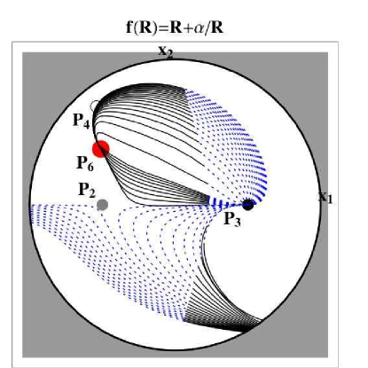
Figure 5: Phase space projected on the plane $(x_{1},x_{2})$ in Poincaré coordinates for the model $f(R)=R+\alpha/R$ in the absence of radiation. For the initial conditions $x_{2}>0$ there are two solutions: either (i) the solutions directly approach the accelerated attractor $P_{6}$ or (ii) they first approach the saddle $\phi$MDE point $P_{2}$ and then reach the attractor $P_{6}$. When $x_{2}<0$ initially, the trajectories moves toward $x_{2}\to-\infty$. Note that the point $P_{3}$ is unstable.

When $n>0$ one has $m=-n-1<-1$ and $m^{\prime}(r)=n/r^{2}>0$ for $P_{5}$ and $P_{6}$. In this case $P_{6}$ is a stable attractor whereas $P_{5}$ is a saddle. In the previous section we showed that the matter point $P_{5}$ is disconnected to the accelerated point $P_{6}$ since $P_{6}$ exists in the region (A). According to the results in Ref. APT we have only the following two cases: either (i) the matter era is replaced by the $\phi$MDE fixed point $P_{2}$ which is followed by the accelerated attractor $P_{6}$, or (ii) a rapid transition from the radiation era to the accelerated attractor $P_{6}$ without the $\phi$MDE. Which trajectories are chosen depend upon the model parameters and initial conditions. In Fig. 5 we depict a 2-dimensional phase space plot for the model $n=1$. This shows that the final attractor is in fact $P_{6}$ and that whether the solutions temporally approach the saddle point $P_{2}$ or not depends on initial conditions.

Figure 6: The cosmic evolution of various quantities is shown for the model $f(R)=R+\alpha/R^{2}$ with $\alpha=-\mu^{6}$, $\mu/H_{0}=11.04$. The standard matter era is replaced by the $\phi$MDE which corresponds to $a\propto t^{1/2}$, $w_{{\rm eff}}=1/3$ and $\Omega_{{\rm m}}=2$. The redshift $z_{a}$ at which acceleration starts is $z_{a}=0.4$ and we have asymptotically in the future $\Omega_{{\rm DE}}=1$ and $w_{{\rm eff}}=w_{{\rm DE}}=-0.82$ [see Eq. (63)].

In order to understand the evolution after the radiation era let us consider the model $n=1$ without radiation. From Eqs. (4) and (5) we find that the evolution of the scale factor during the $\phi$MDE is given by

$$a(t)=(t/t_{i})^{1/2}+\epsilon(t)(t/t_{i})^{9/4}\,,$$ (79)

where the subscript ‘i’ represents the value at the beginning of the $\phi$MDE. At first order in $\epsilon(t)$ we have

$$\epsilon(t)=\frac{\mu^{2}}{144H_{i}^{2}}\frac{1}{\sqrt{\rho_{m}^{(i)}/3H_{i}^{2}-(H/H_{i})^{1/2}}}\,.$$ (80)

Notice that $\mu$ is of order $H_{0}$ to realize the present acceleration. Since $H_{0}\ll H_{i}$ the parameter $\epsilon(t)$ is in fact much smaller than unity. The scale factor evolves as $a\propto t^{1/2}$ during the $\phi$MDE, but this epoch ends when the second term in Eq. (79) gets larger than the zero-th order term. Hence the end of the $\phi$MDE is characterized by

$$t\approx\left(\frac{144H_{i}^{2}}{\mu^{2}}\sqrt{\frac{\rho_{m}^{(i)}}{3H_{i}^{2}}}\right)^{4/7}\,t_{i}\,.$$ (81)

After that the solutions approach the accelerated attractor $P_{5}$. Equation (81) shows that the duration of the $\phi$MDE depends on $\mu$ together with the initial conditions $\rho_{m}^{(i)}$ and $H_{i}$. The similar argument can be applied for any $n<-1,n>-3/4$ with a correction growing as $t^{5/2-1/2(n+1)}$. In Fig. 6 we plot the evolution of various quantities for $n=2$. In this case the radiation era is followed by the $\phi$MDE saddle point $P_{2}$ with $\Omega_{{\rm m}}=2$ and $w_{{\rm eff}}=1/3$. The final attractor is the accelerated point $P_{6}$ with $\Omega_{{\rm DE}}=1$ and $w_{{\rm eff}}=-0.82$. As is clearly seen in the right panel of Fig. 6 we do not have a standard matter era with $w_{{\rm eff}}=0$.

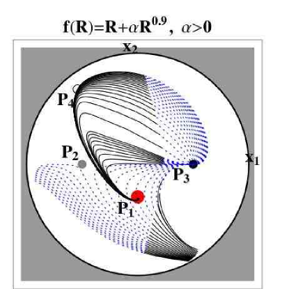
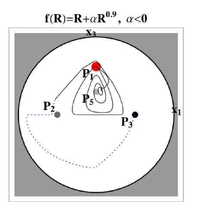
Figure 7: Projected phase space in Poincaré coordinates for the model $f(R)=R+\alpha R^{0.9}$ in the absence of radiation. The final attractor is the de-Sitter point $P_{1}:(x_{1},x_{2},x_{3})=(0,-1,2)$. Note that both $P_{2}$ and $P_{6}$ are not stable unlike the model $f(R)=\alpha R^{0.9}$. In the left panel, $\alpha>0$: here $P_{5}$ corresponds to $m<0$ with a large eigenvalue and therefore is unstable. In the right panel, $\alpha<0$: now the point $P_{5}$ is a saddle with positive $m$, so it is possible to have a sequence of an oscillating matter phase followed by the late-time acceleration. We plot a single curve for clarity.

Let us consider the case in which $n$ is close to $-1$. When $n<-1$ the point $P_{5}$ is a stable spiral, so the matter era is not followed by an accelerated expansion as is similar to the power-law models. If $n>-1$, the de-Sitter point $P_{1}$ is stable whereas the phantom point $P_{6}$ is not. In Fig. 7 we show the phase space plot in a two-dimensional plane for $n=-0.9$. When $\alpha>0$, although the point $P_{5}$ is a saddle, the solutions approach the attractor $P_{1}$ without staying the region around the point $P_{5}$ for a long time because $m$ is negative. This tendency is more significant if $n$ is chosen to be closer to $-1$, i.e. $m\to-0$. Hence one can not have a prolonged matter era in these cases as well. On the other hand, for $\alpha<0$, we have $m\to+0$ and there are oscillations around the matter era followed again by the attractor $P_{1}$. Then this latter case, belonging to Class II, can be cosmologically viable.

VI.3 $f(R)=R(\log\alpha R)^{q}$

When $q>0$, we showed that the point $P_{5}$ is a saddle for $m(r<-1)>0$ whereas both $P_{1}$ and $P_{6}$ are stable. In the previous section we showed that the only possibility is the trajectory from $P_{5}$ to $P_{1}$. Hence the solutions starting from the radiation era reach the saddle matter point $P_{5}$ first, which is followed by the de-Sitter point $P_{1}$.

In order to obtain a prolonged matter period, the variables $m$ and $r$ need to be close to $+0$ and $r=-1$, respectively, at the end of radiation era. If we integrate the autonomous equations with initial conditions $r=x_{3}/x_{2}\simeq-1$ (and smaller than $-1)$ and $x_{4}\simeq 1$, we find that the matter era is too long to be compatible with observations. In Fig. 8 we plot one example of such cosmological evolution for $q=1$. This shows that a prolonged (quasi) matter era certainly exists prior to the late-time acceleration. The final attractor is the de-Sitter point $P_{1}$ with $w_{{\rm eff}}=-1$. However in this case the beginning of the matter epoch corresponds to the redshift $z=1.1\times 10^{17}$, which is much larger compared to the standard value $z\sim 10^{3}$. The present value of the radiation energy fraction is $\Omega_{{\rm rad},0}=2.8\times 10^{-15}$ and is much smaller than the value given in Eq. (78).

This unusually long period of the matter era is associated with the fact that the point $P_{5}$ is a saddle in the region $r<-1$ but it is marginally stable in the limit $r\to-1$ (i.e. $m\to+0$). Hence as we choose the initial values of $r$ closer to $-1$, the duration of the matter period gets longer. In order to recover the present value of $\Omega_{{\rm rad}}$ given in Eq. (78), we have to make the matter period shorter by appropriately choosing initial conditions at the end of the radiation era. In Fig. 9 we plot the cosmological evolution in the case where the end of the radiation era corresponds to $z\sim 10^{3}$ with present values $\Omega_{{\rm m,0}}\approx 0.3$ and $\Omega_{{\rm rad,0}}\approx 10^{-4}$. The energy fraction of the matter is not large enough to dominate the universe after the radiation epoch. Hence this case is not compatible with observations as well.

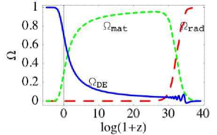
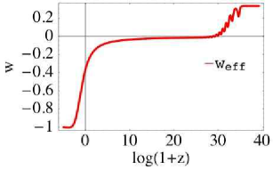
Figure 8: The cosmic evolution of various quantities for the model $f(R)=R{\rm log}\,\alpha R$ with initial conditions $x_{1}=10^{-5}$, $x_{2}=-10^{-10}$, $x_{3}=1.01\times 10^{-10}$ and $x_{4}=0.999$ at the redshift $z=1.1\times 10^{17}$, corresponding to $r=-1.01$. In this case the matter era is too long relative to the standard cosmology. In fact the energy fraction of the radiation at the present epoch is $\Omega_{{\rm rad},0}=2.8\times 10^{-15}$, which is much smaller than the standard value $\Omega_{{\rm rad},0}\approx 10^{-4}$.

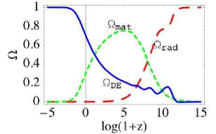
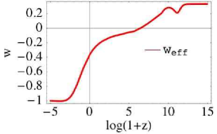
Figure 9: The cosmic evolution of various quantities for the model $f(R)=R{\rm log}\,\alpha R$ with initial conditions $x_{1}=10^{-10}$, $x_{2}=-10^{-7}$, $x_{3}=1.019\times 10^{-7}$ and $x_{4}=0.999$ at the redshift $z=3.15\times 10^{6}$, corresponding to $r=-1.019$. In this case we have $\Omega_{{\rm m,0}}\approx 0.3$ and $\Omega_{{\rm rad,0}}\approx 10^{-4}$ at the present epoch, but the matter era is practically absent.

VI.4 $f(R)=R\exp(q/R)$

In this case the matter point $P_{5}$ is a saddle, but one of the eigenvalues are 3 rather than close to 0. Numerically we find that the solutions do not reach the matter dominated epoch unlike the $f(R)=R(\log\alpha R)^{q}$ model with $q>0$. In Fig. 10 we plot the cosmological evolution for this model corresponding to the present values $\Omega_{{\rm m,0}}\approx 0.3,\Omega_{{\rm rad,0}}\approx 10^{-4}$. In this case the matter epoch is replaced by the $\phi$MDE. It is possible to find a situation in which there exists a short period of the matter era, but we find that this case does not satisfy the conditions given by (78). Thus this model is not cosmologically viable in spite of the fact that it belongs to the Class II.

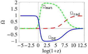
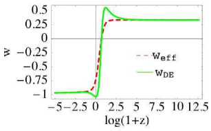
Figure 10: The cosmic evolution of various quantities for the model $f(R)=R\exp(q/R)$ with initial conditions $x_{1}=0$, $x_{2}=2.13\times 10^{-20}$, $x_{3}=5.33\times 10^{-21}$ and $x_{4}=0.99$ at the redshift $z=3\times 10^{5}$. We see that the matter era is absent and is replaced by the $\phi$MDE.

VI.5 $m(r)=-0.2(1+r)(3.2+0.8r+r^{2})$

This model belongs to the Class IV, so the cosmological trajectories can be acceptable. In Fig. 11 we find that the matter epoch is in fact followed by a stable acceleration with $w_{{\rm eff}}\approx-0.935$. The transition between the various eras is not very sharp compared to the $\Lambda$CDM model, so it is of interest to investigate in more detail whether this model can be really compatible with observations. However this is beyond the scope of this paper.

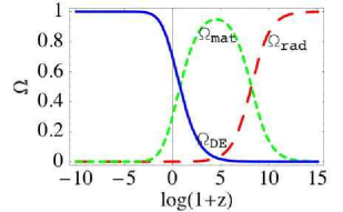
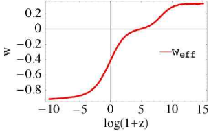
Figure 11: The cosmic evolution of various quantities for the model $m(r)=-0.2(1+r)(3.2+0.8r+r^{2})$ with initial conditions $x_{1}=10^{-10}$, $x_{2}=-10^{-7}$, $x_{3}=1.000007\times 10^{-7}$ and $x_{4}=0.999$ at the redshift $z=3.5\times 10^{6}$. The model has an approximate matter dominated epoch followed by a non-phantom accelerated universe with $w_{{\rm eff}}\approx-0.935$.

VII Conclusions

The $f(R)$ dark energy models are interesting and quite popular attempts to explain the late-time acceleration. However it was recently found that the popular model $f(R)=R+\alpha R^{-n}$ with $n>0$ is unable to produce a matter era prior to the accelerated epoch APT . In this paper we have attempted to clarify the conditions under which $f(R)$ dark energy models are cosmologically viable. We first derived the autonomous equations (26)-(29) which are applicable to general $f(R)$ models. In Sec. III all fixed points are derived in such an autonomous system. By considering linear perturbations about the fixed points, we have studied their stabilities to understand the cosmological evolution in $f(R)$ dark energy models.

The main result of this paper is that we have identified four classes of $f(R)$ models, depending on the existence of a standard or “wrong” matter era ($\phi$MDE) and on the final acceleration. In practice, we have shown that the cosmology of $f(R)$ models can be based on a study of the $m(r)$ curves in the $(r,m)$ plane and on its intersections with the critical line $m=-r-1$. This provides an extremely simple method to investigate the cosmological viability of such models. In particular, we find that the Class I models correspond to the type of models in which the final acceleration is preceded by a so-called $\phi$MDE phase characterized by $a\propto t^{1/2}$ or in which the matter phase does not exist at all prior to the accelerated epoch. These models are clearly ruled out, e.g. by the angular diameter distance of the CMB acoustic peaks, see Ref. APT . This is by far the largest class and only a few special cases belong to other three.

The general conditions for a successful $f(R)$ model can be summarized as follows:

• A $f(R)$ model has a standard matter dominated epoch only if it satisfies the conditions

  $$m(r)\approx+0\quad{\rm and}\quad m^{\prime}(r)>-1\quad{\rm at}\quad r\approx-1\,,$$ (82)

  where the second condition is required to leave the matter era for the late-time acceleration.

• The matter epoch is followed by a de-Sitter acceleration ($w_{{\rm eff}}=-1$) only if

  $$0\leq m(r)\leq 1\quad{\rm at}\quad r=-2\quad{\rm or}\quad m(r)=-r-1\to\pm\infty\quad({\rm Class\leavevmode\nobreak\ II})\,.$$ (83)

• The matter epoch is followed by a non-phantom accelerated attractor ($w_{{\rm eff}}\geq-1$) only if $m=-r-1$ and

  $$(\sqrt{3}-1)/2<m(r)\leq 1\quad{\rm and}\quad m^{\prime}(r)<-1\quad({\rm Class\leavevmode\nobreak\ IV})\,.$$ (84)

Moreover, the curve $m(r)$ must connect with continuity the vicinity of the matter point $P_{5}:(r,m)=(-1,0)$ with one of the accelerated regions. The Class II and IV models are characterized by $m(r)$ curves that satisfy these requirements and lead therefore to an acceptable cosmology.

In the Class III models the curve $m(r)$ intersects the critical line at $m$ small and negative. In this case the saddle eigenvalue takes a very large real value and the matter era is practically unstable and therefore generically very short. Moreover, most trajectories will be attracted by the strongly phantom attractor with $w_{{\rm eff}}<-7.6$ which is in contrast with observations.

The cases with $m^{\prime}(r)=-1$ or $m^{\prime}(r)\to\pm\infty$ at the critical points are not covered in our linear approach and a higher-order or numerical analysis is necessary. Also the power-law model $f(R)=R^{-n}$ is a rather special case in a sense that it gives a transition from the quasi matter era to the strongly phantom epoch with a constant negative $m$. However we showed that this model is not cosmologically acceptable because of the absence of the prolonged matter epoch. We have also studied analytically and numerically models like $f(R)=R+\alpha R^{-n},R^{p}(\log\alpha R)^{q},R^{p}\exp(qR),R^{p}\exp(q/R),(R^{a}-\Lambda)^{b}$ and others and have confirmed the conclusions drawn from the $m(r)$ approach. See Table I for the summary of the classification of a sample of $f(R)$ dark energy models.

As we have seen, the variable $m=Rf_{,RR}/f_{,R}$ plays a central role to determine the cosmological viability of $f(R)$ dark energy models. The $\Lambda$CDM model, $f(R)=R-\Lambda$, corresponds to $m=0$ at all times, which thus satisfies the condition for the existence of the matter era ($m\approx 0$) followed by the de-Sitter point at $m(r=-2)=0$. The difference from the line $m=0$ characterises the deviation from the $\Lambda$CDM model. If the devaition from $m=0$ is small, it is expected that such models are cosmologically viable.

We conclude with a comment concerning a possible signature of $f(R)$ cosmology. The standard matter era can be realized with $m\to\pm 0$. As we have seen, in all successful cases we analyzed in this work, the matter era is realized through damped oscillations with positive $m$. This raises the obvious question of whether such oscillations are observable and whether they could be taken as a signature of modified gravity. This question is left to future work. An additional interesting direction to investigate is the evolution of cosmological perturbations in $f(R)$ dark energy models in order to confront with the datasets of CMB and large scale structure along the lines of Refs. Song ; Bean ; FTBM06 .

References

- (1) V. Sahni and A. A. Starobinsky, Int. J. Mod. Phys. D 9, 373 (2000); S. M. Carroll, Living Rev. Rel. 4, 1 (2001); T. Padmanabhan, Phys. Rept. 380, 235 (2003); P. J. E. Peebles and B. Ratra, Rev. Mod. Phys. 75, 559 (2003); V. Sahni, Lect. Notes Phys. 653, 141 (2004) [arXiv:astro-ph/0403324].
- (2) E. J. Copeland, M. Sami and S. Tsujikawa, Int. J. Mod. Phys. D 15, 1753 (2006).
- (3) S. Perlmutter et al., Astrophys. J. 517, 565 (1999); A. G. Riess et al., Astron. J. 116, 1009 (1998); Astron. J. 117, 707 (1999); J. L. Tonry et al., Astrophys. J. 594, 1 (2003); R. A. Knop et al., Astrophys. J. 598, 102 (2003).
- (4) D. N. Spergel et al., Astrophys. J. Suppl. 148, 175 (2003); D. N. Spergel et al., arXiv:astro-ph/0603449.
- (5) M. Tegmark et al., Phys. Rev. D 69, 103501 (2004); U. Seljak et al., Phys. Rev. D 71, 103515 (2005).
- (6) D. J. Eisenstein et al., Astrophys. J. 633, 560 (2005); C. Blake, D. Parkinson, B. Bassett, K. Glazebrook, M. Kunz and R. C. Nichol, Mon. Not. Roy. Astron. Soc. 365, 255 (2006).
- (7) B. Jain and A. Taylor, Phys. Rev. Lett. 91, 141302 (2003).
- (8) U. Seljak, A. Slosar and P. McDonald, JCAP 0610, 014 (2006).
- (9) P. Astier et al., Astron. Astrophys. 447, 31 (2006).
- (10) M. Chevallier and D. Polarski, Int. J. Mod. Phys. D 10, 213 (2001).
- (11) V. Sahni and A. A. Starobinsky, arXiv:astro-ph/0610026.
- (12) Y. Fujii, Phys. Rev. D 26, 2580 (1982); L. H. Ford, Phys. Rev. D 35, 2339 (1987); C. Wetterich, Nucl. Phys B. 302, 668 (1988); B. Ratra and J. Peebles, Phys. Rev D 37, 321 (1988); Y. Fujii and T. Nishioka, Phys. Rev. D 42, 361 (1990); E. J. Copeland, A. R. Liddle, and D. Wands, Ann. N. Y. Acad. Sci. 688, 647 (1993); C. Wetterich, A&A 301, 321 (1995); P. G. Ferreira and M. Joyce, Phys. Rev. Lett. 79, 4740 (1997); Phys. Rev. D 58, 023503 (1998); R. R. Caldwell, R. Dave and P. J. Steinhardt, Phys. Rev. Lett. 80, 1582 (1998); I. Zlatev, L. M. Wang and P. J. Steinhardt, Phys. Rev. Lett. 82, 896 (1999); P. J. Steinhardt, L. M. Wang and I. Zlatev, Phys. Rev. D 59, 123504 (1999).
- (13) L. Amendola, Phys. Rev. D 62, 043511 (2000); L. Amendola and D. Tocchini-Valentini, Phys. Rev. D 64, 043509 (2001); L. Amendola and C. Quercellini, Phys. Rev. D 68, 023514 (2003).
- (14) L. Amendola, M. Quartin, S. Tsujikawa and I. Waga, Phys. Rev. D 74, 023525 (2006).
- (15) A. Melchiorri, L. Mersini-Houghton, C. J. Odman and M. Trodden, Phys. Rev. D 68, 043509 (2003); U. Alam, V. Sahni, T. D. Saini and A. A. Starobinsky, Mon. Not. Roy. Astron. Soc. 354, 275 (2004); B. A. Bassett, P. S. Corasaniti and M. Kunz, Astrophys. J. 617, L1 (2004).
- (16) R. R. Caldwell, Phys. Lett. B 545,23-29 (2002); R. R. Caldwell, M. Kamionkowski and N. N. Weinberg, Phys. Rev. Lett. 91, 071301 (2003); S. M. Carroll, M. Hoffman and M. Trodden, Phys. Rev. D 68, 023509 (2003); P. Singh, M. Sami and N. Dadhich, Phys. Rev. D 68 023522 (2003).
- (17) J. M. Cline, S. Jeon and G. D. Moore, Phys. Rev. D 70, 043543 (2004); N. Arkani-Hamed, H. C. Cheng, M. A. Luty and S. Mukohyama, JHEP 0405, 074 (2004); F. Piazza and S. Tsujikawa, JCAP 0407, 004 (2004).
- (18) J. P. Uzan, Phys. Rev. D 59, 123510 (1999); L. Amendola, Phys. Rev. D 60, 043501 (1999); T. Chiba, Phys. Rev. D 60, 083508 (1999);
- (19) Y. Fujii, Phys. Rev. D62, 044011 (2000); N. Bartolo and M. Pietroni, Phys. Rev. D 61 023518 (2000); F. Perrotta, C. Baccigalupi and S. Matarrese, Phys. Rev. D 61, 023507 (2000); A. Riazuelo & J.-P. Uzan, Phys.Rev. D66 (2002) 023525
- (20) G. Esposito-Farèse and D. Polarski, Phys. Rev. D 63 063504 (2001).
- (21) B. Boisseau, G. Esposito-Farèse, D. Polarski and A. A. Starobinsky, Phys. Rev. Lett. 85, 2236 (2000).
- (22) R. Gannouji, D. Polarski, A. Ranquet and A. A. Starobinsky, JCAP 0609, 016 (2006).
- (23) L. Perivolaropoulos, JCAP 0510, 001 (2005); S. Nesseris and L. Perivolaropoulos, arXiv:astro-ph/0610092.
- (24) S. Capozziello, V. F. Cardone, S. Carloni and A. Troisi, Int. J. Mod. Phys. D 12, 1969 (2003).
- (25) S. M. Carroll, V. Duvvuri, M. Trodden and M. S. Turner, Phys. Rev. D 70, 043528 (2004).
- (26) S. Capozziello, F. Occhionero and L. Amendola, Int. J. Mod. Phys. D 1 (1993) 615.
- (27) T. Chiba, Phys. Lett. B 575, 1 (2003).
- (28) A. D. Dolgov and M. Kawasaki, Phys. Lett. B 573, 1 (2003).
- (29) V. Faraoni, Phys. Rev. D 74, 023529 (2006).
- (30) S. Nojiri and S. D. Odintsov, Phys. Rev. D 68, 123512 (2003).
- (31) A. W. Brookfield, C. van de Bruck and L. M. H. Hall, Phys. Rev. D 74, 064028 (2006).
- (32) I. Navarro and K. Van Acoleyen, arXiv:gr-qc/0611127.
- (33) F. Perrotta and C. Baccigalupi, Phys. Rev. D 65, 123505 (2002); S. Nojiri and S. D. Odintsov, Gen. Rel. Grav. 36, 1765 (2004); M. E. Soussa and R. P. Woodard, Gen. Rel. Grav. 36, 855 (2004); G. Allemandi, A. Borowiec and M. Francaviglia, Phys. Rev. D 70, 103503 (2004); D. A. Easson, Int. J. Mod. Phys. A 19, 5343 (2004); S. M. Carroll, A. De Felice, V. Duvvuri, D. A. Easson, M. Trodden and M. S. Turner, Phys. Rev. D 71, 063513 (2005); S. Carloni, P. K. S. Dunsby, S. Capozziello and A. Troisi, Class. Quant. Grav. 22, 4839 (2005); S. Capozziello, V. F. Cardone and A. Troisi, Phys. Rev. D 71, 043503 (2005); G. Cognola, E. Elizalde, S. Nojiri, S. D. Odintsov and S. Zerbini, JCAP 0502, 010 (2005); S. Nojiri, S. D. Odintsov and S. Tsujikawa, Phys. Rev. D 71, 063004 (2005); M. C. B. Abdalla, S. Nojiri and S. D. Odintsov, arXiv:hep-th/0601213; R. P. Woodard, arXiv:astro-ph/0601672; S. Das, N. Banerjee and N. Dadhich, Class. Quant. Grav. 23, 4159 (2006); S. Capozziello, V. F. Cardone, E. Elizalde, S. Nojiri and S. D. Odintsov, Phys. Rev. D 73, 043512 (2006); S. K. Srivastava, arXiv:astro-ph/0602116; T. P. Sotiriou, Class. Quant. Grav. 23, 5117 (2006); arXiv:gr-qc/0611107; arXiv:gr-qc/0611158; T. P. Sotiriou and S. Liberati, arXiv:gr-qc/0604006; A. De Felice, M. Hindmarsh and M. Trodden, JCAP 0608, 005 (2006); S. Nojiri and S. D. Odintsov, Phys. Rev. D 74, 086005 (2006); A. de la Cruz-Dombriz and A. Dobado, Phys. Rev. D 74, 087501 (2006); S. Bludman, arXiv:astro-ph/0605198; S. M. Carroll, I. Sawicki, A. Silvestri and M. Trodden, New J. Phys. 8, 323 (2006); D. Huterer and E. V. Linder, Phys. Rev. D 75, 023519 (2007); V. Faraoni, Phys. Rev. D 74, 104017 (2006); V. Faraoni and S. Nadeau, Phys. Rev. D 75, 023501 (2007); X. h. Jin, D. j. Liu and X. z. Li, arXiv:astro-ph/0610854; N. J. Poplawski, Phys. Rev. D 74, 084032 (2006); arXiv:gr-qc/0610133; A. F. Zakharov, A. A. Nucita, F. De Paolis and G. Ingrosso, Phys. Rev. D 74, 107101 (2006); T. Chiba, T. L. Smith and A. L. Erickcek, arXiv:astro-ph/0611867; E. O. Kahya and V. K. Onemli, arXiv:gr-qc/0612026; S. Fay, R. Tavakol and S. Tsujikawa, arXiv:astro-ph/0701479; M. Fairbairn and S. Rydbeck, arXiv:astro-ph/0701900; G. Cognola, M. Gastaldi and S. Zerbini, arXiv:gr-qc/0701138; B. Li and J. D. Barrow, arXiv:gr-qc/0701111; T. Rador, arXiv:hep-th/0701267; I. Sawicki and W. Hu, arXiv:astro-ph/0702278; S. Fay, S. Nesseris and L. Perivolaropoulos, arXiv:gr-qc/0703006.
- (34) L. Amendola, D. Polarski and S. Tsujikawa, arXiv:astro-ph/0603703, Physical Review Letters to appear.
- (35) J. Barrow and A. Ottewill, J. Phys. A 16, 2757 (1983).
- (36) A. A. Starobinsky, Phys. Lett. B 91, 99 (1980).
- (37) J. c. Hwang, Astrophys. J. 375, 443 (1991).
- (38) D. F. Torres, Phys. Rev. D 66, 043522 (2002).
- (39) D. Polarski and A. Ranquet, Phys. Lett. B 627, 1 (2005).
- (40) S. Capozziello, S. Nojiri, S. D. Odintsov and A. Troisi, Phys. Lett. B 639, 135 (2006).
- (41) L. Amendola, D. Polarski and S. Tsujikawa, arXiv:astro-ph/0605384.
- (42) S. Capozziello, V. F. Cardone and A. Troisi, Phys. Rev. D 71, 043503 (2005).
- (43) J. Barrow and T. Clifton, Phys. Rev D 72, 103005 (2005).
- (44) Y. S. Song, W. Hu and I. Sawicki, arXiv:astro-ph/0610532.
- (45) R. Bean, D. Bernat, L. Pogosian, A. Silvestri and M. Trodden, arXiv:astro-ph/0611321.
- (46) T. Faulkner, M. Tegmark, E. F. Bunn and Y. Mao, arXiv:astro-ph/0612569.