General Relativistic Radiant Shock Waves in the Post-Quasistatic Approximation

Abstract

An evolution of radiant shock wave front is considered in the framework of a recently presented method to study self–gravitating relativistic spheres, whose rationale becomes intelligible and finds full justification within the context of a suitable definition of the post–quasistatic approximation. The spherical matter configuration is divided into two regions by the shock and each side of the interface having a different equation of state and anisotropic phase. In order to simulate dissipation effects due to the transfer of photons and/or neutrinos within the matter configuration, we introduce the flux factor, the variable Eddington factor and a closure relation between them. As we expected the strength of the shock increases the speed of the fluid to relativistic values and for some critical ones is larger than light speed. In addition, we find that energy conditions are very sensible to the anisotropy, specially the strong one. As a special feature of the model , we find that the contribution of the matter and radiation to the radial pressure are the same order of magnitude as in the mant as in the core, moreover, in the core radiation pressure is larger than matter pressure.

1 Introduction

During the implosion that forms a relativistic compact object, nearly all of its gravitational binding energy ($({GM^{2}})/{R}\sim 5\times 10^{53}$ ergs $\sim 0.2Mc^{2}$) is stored as internal energy of a proto-neutron star and driven by neutrino diffusion. Roughly speaking, there is a consensus that this collapsing scenario requires, three main “ingredients” [1]:

1. a copious emission of radiation, been a consequence of the microphysics of the system, tends to abandon the system, but the absorption and the scattering in the medium hinder it to escape freely.

2. phase transitions that can induce local anisotropic pressures (i.e. $P_{r}\neq P_{\perp}$). An increasing amount of theoretical evidence strongly suggests that, for certain density ranges, a variety of very interesting physical phenomena may take place giving rise to local anisotropy (see [2, 3] and [4, 5, 6, 7, 8, 9, 10, 11, 12, 13] for more recent studies ).

3. the formation and propagation of a surface of discontinuity: a shock wave, a detonation or combustion front (deflagration or slow combustion) having width very small compared to the size of the system.

Although now exist several independent numerical codes which provide accurate modeling of gravitational collapse in full General Relativity (see [14] for a good review on this subject and/or visit some these links concerning codes for simulations [15] ), none of these codes provide all the above mentioned “ingredient”.

In order to explore the influence that the scheme of radiation and the local anisotropy exert on the propagation of a surface of discontinuity, we shall follow a “seminumerical” approach which starting from a known interior (analytical) static spherically symmetric ( considered as “seed”) solution to the Tolman-Oppenheimer-Volkov equation. It can be considered as a continuation of previous studies [25, 26, 27]. This scheme transforms the Einstein partial differential equations into a system of ordinary differential equations for quantities evaluated at the surfaces (boundary & shock). It is an extension of the so called HJR method [16], which has been successfully applied to a variety of astrophysical scenarios (see [24] and references therein) and which has been recently revisited [17, 18, 19].

When considering the interaction between radiation and ultradense matter, we consider two quantities: the flux factor, $f={\mathcal{F}}/{\rho_{R}},$ and the variable Eddington factor, $\chi=P_{R}/{\rho_{R}},$ and a closure relation between them, i.e., $\chi=\chi(f)$ (see [20, 21, 22, 23] ), where ${\cal F}$, $\rho_{R}$ and $P_{R}$ are the radiation flux, and the contribution of the radiation to the energy density and radial pressure.

Here we shall show that the strength of the shock appears to be a very significant feature concerning the evolution of the distribution, because it drastically increases the fluid velocity behind the shock. We have also found that the energy conditions (specially the strong one) are very sensitive to the variation of the local anisotropy, and hydrodynamic & radiation pressures emerge of the same order of magnitude and even, at the core, radiation pressure is larger than that of matter counter part.

This paper is organized as follows: in section 2 the energy-momentum tensor and field equations for a non-static spherically symmetric fluid with matter and radiation are established. The Post-Quasistatic approximation is considered in section 3 Section 4 is devoted to describe the Taub junction conditions across the surface of discontinuity. Finally, we end this work with discussing some the results of the numerical simulations.

2 Matter, radiation and field equations

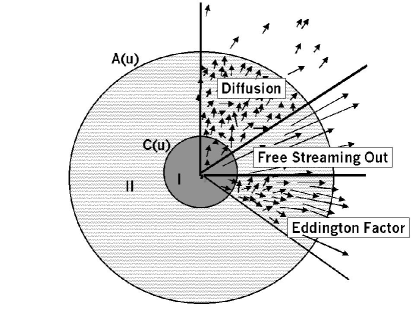
As it can be appreciated in Figure 1, the collapsing configuration is described by three regions: a core ($I$) as the more inner region, the mantle ($II$) in the middle, and the outer space labeled by ($III$).

Core and mantle are separated by mean of a shock (discontinuity hypersurface) and a boundary surface (hypersurface with velocity equal to the fluid in these point) is define the matter configuration. Both the shock and the boundary surface are time-like hypersurfaces and there only exists unpolarized radiation emerging which is modeled by the radiative Vaidya exterior metric.

Figure 1: Regions of the matter distribution. The core is labeled by $I$ is the more compact one; the mantle ($II$) is the region in the middle and the exterior space–time ($III$).

The line elements at each region are

$$ds^{2}_{I,II}=e^{\nu}dt^{2}-e^{\lambda}dr^{2}-r^{2}(d\theta^{2}+\sin^{2}\theta d\phi^{2}),$$ (1)

and

$$ds^{2}_{III}=\left(1-\frac{2M(u)}{R}\right)du^{2}+2dudR-R^{2}(d\theta^{2}+\sin^{2}\theta d\phi^{2})\,,$$ (2)

where $\nu$ and $\lambda$ are functions of $t$ and $r$, $u$ is the retarded time and $R$ is a null coordinate ($g_{RR}=0$).

For a comoving observer with radial velocity $\omega$ relative to local Minkowskian coordinates, the physical content of the fluid is represented by the radiation flux ${\cal F}$ in the radial direction; the energy density $\bar{\rho}$ and $\bar{P}_{r}$, and $\bar{P}_{\bot}$ as the radial and tangential pressures, respectively. The bar stands for the total (hydrodynamic $+$ radiation) contribution. Thus, the energy-momentum tensor for each region can be written as,

$$(T_{\alpha\beta})_{I,II} = (\bar{\rho}+\bar{P}_{\bot})u_{\alpha}u_{\beta}-\bar{P}_{\bot}g_{\alpha\beta}+(\bar{P}-\bar{P}_{\bot})\chi_{\alpha}\chi_{\beta}+2{\cal F}_{(\alpha}u_{\beta)}$$

$$(T_{\alpha\beta})_{III} = -\frac{1}{4\pi R^{2}}\frac{dM}{du}\delta^{0}_{\alpha}\delta^{0}_{\beta}$$ (3)

where [28]

$$\bar{\rho} = \rho+\rho_{R}\,,\quad\bar{P}=P_{r}+P_{R}\,,\quad\bar{P}_{\bot}=P_{\bot}+(P_{\bot})_{R}\,,\quad(P_{\bot})_{R}=\frac{\rho_{R}-P_{R}}{2}\,,$$ (4)

$$u_{\alpha} = \frac{e^{\nu/2}\delta^{0}_{\alpha}-\omega e^{\lambda/2}\delta^{1}_{\alpha}}{\sqrt{1-\omega^{2}}}\,,\quad\chi_{\alpha}=\frac{-\omega e^{\nu/2}\delta^{0}_{\alpha}+e^{\lambda/2}\delta^{1}_{\alpha}}{\sqrt{1-\omega^{2}}}\,,\quad{\cal F}_{\alpha}=-{\cal F}\chi_{\alpha}\,,$$ (5)

with the subscript $R$ denoting the contribution of the radiation.

For the above energy-momentum tensor, Einstein field equations $G^{\alpha}_{\hphantom{\alpha}\beta}=-8\pi T^{\alpha}_{\hphantom{\alpha}\beta}$ become

$$-8\pi\left(\frac{\bar{\rho}+\omega^{2}\bar{P}+2\omega{\cal F}}{1-\omega^{2}}\right)=-\frac{1}{r^{2}}+e^{-\lambda}\left(\frac{1}{r^{2}}-\frac{\lambda^{\prime}}{r}\right)\,,$$ (6)

$$-8\pi\left(\frac{\bar{P}+\omega^{2}\bar{\rho}+2\omega{\cal F}}{1-\omega^{2}}\right)=-\frac{1}{r^{2}}+e^{-\lambda}\left(\frac{1}{r^{2}}+\frac{\nu^{\prime}}{r}\right)\,,$$ (7)

$$-8\pi\bar{P}_{\bot}=\frac{e^{-\nu}}{4}\left[2\ddot{\lambda}+\dot{\lambda}(\dot{\lambda}-\dot{\nu})\right]-\frac{e^{-\lambda}}{4}\left[2\nu^{\prime\prime}+\left(\nu^{\prime}+\frac{2}{r}\right)(\nu^{\prime}-\lambda^{\prime})\right]\,,$$ (8)

$$-8\pi e^{\frac{\nu+\lambda}{2}}\left[\frac{\omega(\bar{\rho}+\bar{P})+(1+\omega^{2}){\cal F}}{1-\omega^{2}}\right]=\frac{\dot{\lambda}}{r}\,,$$ (9)

where dots and primes are denoting time and radial derivatives, respectively.

3 The Post–Quasistatic Approximation (PQA)

The quasistatic regime is “the next step coming out from hydrostatic equilibrium”. In this regime the distribution changes slowly in a typical time scale which is very long compared with the characteristic scale within the sphere reacts to a perturbation. Mathematically, it can be stated as [18] ${\cal O}(\omega^{2})=\ddot{\lambda}=\ddot{\nu}=\dot{\lambda}\dot{\nu}=\dot{\lambda}^{2}=\dot{\nu}^{2}=0\,.$

Now, we define the “efective variables”

$$\tilde{\rho}=\frac{\bar{\rho}+\bar{P}\omega^{2}+2\omega{\cal F}}{1-\omega^{2}}\qquad\mathrm{and}\qquad\tilde{P}=\frac{\bar{P}+\bar{\rho}\omega^{2}+2\omega{\cal F}}{1-\omega^{2}}\,,$$ (10)

which satisfy the same set of equations as their corresponding physical variables in the quasistatic case. Thus, Herrera et al. [18] define the post-quasistatic regime as that corresponding to a system out of equilibrium (or quasiequilibrium) but whose effective variables share the same radial dependence as the physical variables in the state of equilibrium (or quasi-equilibrium), i.e., is the closest possible situation to a quasistatic evolution.

In this effective variables, the field equations (6)–(9) can be written as

$$m = \int 4\pi r^{2}\tilde{\rho}dr\,,$$ (11)

$$\nu = \int\frac{2(4\pi r^{3}\tilde{P}+m)}{r(r-2m)}dr\,,$$ (12)

$$-8\pi\bar{P}_{\bot} = \frac{e^{-\nu}}{4}\left[2\ddot{\lambda}+\dot{\lambda}(\dot{\lambda}-\dot{\nu})\right]-\frac{e^{-\lambda}}{4}\left[2\nu^{\prime\prime}+\left(\nu^{\prime}+\frac{2}{r}\right)(\nu^{\prime}-\lambda^{\prime})\right]\,,$$ (13)

$$\dot{m} = -\frac{4\pi r^{2}e^{\frac{\nu-\lambda}{2}}}{1+\omega^{2}}[\omega(\tilde{\rho}+\tilde{P})+(1-\omega^{2}){\cal F}]\,,$$ (14)

where the mass function is defined by $e^{-\lambda}=1-\frac{2m(t,r)}{r}\,.$

4 Collapsing Model with Shock wave in the PQA

4.1 The regions and the equations of state

Following Herrera and collaborators [25, 27], we consider the core equation of state inspired by the anisotropic Schwarzschild-like interior solution, i.e. [2, 29]

$$\tilde{\rho}_{I}=f(t)\qquad\mathrm{and}\qquad\tilde{P}_{I}=\tilde{\rho}_{I}\left\{\frac{3(1-8/3\pi r^{2}\tilde{\rho}_{I})^{\xi_{I/2}}k(t)-1}{3-(1-8/3\pi r^{2}\tilde{\rho}_{I})^{\xi_{I/2}}k(t)}\right\}\,,$$ (15)

where $\xi_{I}=1-2h_{I}$ is the anisotropic parameter with $h_{I}=0$ corresponding to an isotropic model. For the mantle we have an anisotropic Tolman VI-like solution, i.e.

$$\tilde{\rho}_{II}=\frac{3g(t)}{r^{2}}\qquad\mathrm{and}\qquad\tilde{P}_{II}=\frac{\tilde{\rho}_{II}}{3}\left[\frac{1-9D(t)r^{\sqrt{4-3\xi_{II}}}}{1-D(t)r^{\sqrt{4-3\xi_{II}}}}\right]\,.$$ (16)

again, $h_{II}$ (or $\xi_{II}=1-2h_{II}$) is the parameter messuring the anisotropy of this region and the time-dependent functions $f(t),k(t),g(t)$ and $D(t)$, are obtained from boundary conditions.

4.2 Junction Conditions

The matching across the boundary surface to the Vaidya metric is obtained though the Darmois-Lichnerowicz junction conditions [30], while across the shock front via relativistic Rankine-Hugoniot conditions [31]. As it was pointed out by Bonnor and Vickers some years ago [30], Darmois-Lichnerowicz conditions are not equivalent to the O’Brien and Synge ones. In the present case, O’Brien and Synge conditions lead to a contact discontinuity (not a shock) forcing the fluid velocity to be continuos across the surface $r=c(t)$. Thus denoting the boundary surface by $\Sigma=r-a(t)=0$, the matching conditions lead

$$e^{\nu_{a(t)}}=e^{-\lambda_{a(t)}}=1-\frac{2M(u)}{a(u)}\qquad\mathrm{and}\qquad\bar{P}_{a(t)}={\cal F}_{a(t)}.$$ (17)

Now, if the shock front is described by $\Gamma=r-c(t)=0$, the continuity of the second fundamental form implies the continuity of the mass flux across the shock, and the continuity of the first fundamental form and the Rankine-Hugoniot conditions, lead to

$$[\nu]_{c(t)}=[\lambda]_{c(t)}=0\,,\qquad\left[e^{(\nu-\lambda)/2}\left\{\frac{\omega(\bar{\rho}+\bar{P})+(1+\omega^{2}){\cal F}}{1-\omega^{2}}\right\}-\dot{c}\tilde{\rho}\right]_{c(t)}=0$$ (18)

$$\mathrm{and}\qquad\left[\dot{c}e^{(\lambda-\nu)/2}\left\{\frac{\omega(\bar{\rho}+\bar{P})+(1+\omega^{2}){\cal F}}{1-\omega^{2}}\right\}-\tilde{P}\right]_{c(t)}=0\,,$$ (19)

with $[X]_{c(t)}\equiv X|_{r=c(t)+}-X|_{r=c(t)-}$, where $+$ stands for ahead from the front shock and $-$ for behind. Now, by using the field equation (14) in equations (18) and (19) we obtain

$$[\dot{m}+4\pi r^{2}\dot{c}\tilde{\rho}]_{c(t)}=0\qquad\mathrm{and}\qquad[\dot{m}\dot{c}e^{\lambda-\nu}+4\pi r^{2}\tilde{P}]_{c(t)}=0\,.$$ (20)

Expanding the mass function in a Taylor series about the shock front, we can get a relation between time and radial derivatives and it implies the jump of the time-derivative of the mass across the shock. i.e.

$$\dot{m}(t,r)|_{c(t)}=\dot{m}(t,c)-\dot{c}m^{\prime}(t,r)|_{c(t)}\quad\Longrightarrow[\dot{m}]_{c(t)}=[-4\pi r^{2}\dot{c}\tilde{\rho}]_{c(t)}\,,$$ (21)

and by using (20) we obtain

$$\dot{c}=e^{\frac{\nu_{c(t)}-\lambda_{c(t)}}{2}}\sqrt{\frac{[\tilde{P}]_{c(t)}}{[\tilde{\rho}]_{c(t)}}}\,.$$ (22)

4.3 Metric Functions and Effective Variables

Let us to introduce the dimensionless variables

$$M=\frac{m_{a}}{m_{a}(0)}\,,\quad A=\frac{a}{m_{a}(0)}\,,\quad F=1-\frac{2M}{A}\,,\quad\Omega=\omega_{a}\,,\quad\mathrm{and}\quad t\to\frac{t}{m_{a}(0)}\,,$$ (23)

where $m_{a}(0)$ is the total initial mass of the distribution, and the physical variables

$$\hat{E}=4\pi a^{2}{\cal F}_{a}\,,\quad L=-\dot{M}\,,\quad\mathrm{and}\quad E=-\frac{\dot{M}}{F}\,,$$ (24)

with $\hat{E}$ the luminosity for a (non)comoving observer and $L$ the luminosity at infinity.

All physical variables can be obtained as functions of the above surface variables $A,F,$ and $\Omega$. Thus, from the boundary conditions (17) we get

$$m_{II}=\frac{Mr}{A}\,,\qquad E=(1+\Omega)\hat{E}\,,$$ (25)

$$\tilde{\rho}_{II}=\frac{1-F}{8\pi r^{2}}\,,\qquad\tilde{P}_{II}=\frac{1-F}{24\pi r^{2}}\left[\frac{\psi-9\chi(r/a)^{\sqrt{4-3\xi_{II}}}}{\psi-\chi(r/a)^{\sqrt{4-3\xi_{II}}}}\right]\,,$$ (26)

$$e^{-\lambda_{II}}=F\,,\qquad e^{\nu_{II}}=F\left\{\frac{r}{a}\left[\frac{\psi-\chi(r/a)^{\sqrt{4-3\xi_{II}}}}{\psi-\chi}\right]^{2/{\sqrt{4-3\xi_{II}}}}\right\}^{\frac{4(1-F)}{3F}}\,,$$ (27)

where

$$\psi=3(3+\Omega)(1-F)6(1+\Omega)E\,,\qquad\chi=(1+3\Omega)(1-F)-6(1+\Omega)E\,.$$

Now, by introducing the shock “force” parameter $N$ $(\tilde{P}_{I})_{c}=N(\tilde{P}_{II})_{c}$, we obtain

$$m_{I}=\frac{Mc}{A}(r/c)^{3}\,,\qquad\tilde{\rho}_{I}=\frac{3M}{4\pi c^{2}A}\,,\qquad\tilde{P}_{I}=\tilde{\rho}_{I}\left\{\frac{3u^{\xi_{I/2}}k(t)-1}{3-u^{\xi_{I/2}}k(t)}\right\}\,,$$ (28)

$$e^{-\lambda_{I}}=1-\frac{2Mc}{Ar}(r/c)^{3}\,,\qquad e^{\nu_{I}}=Hu^{\Phi}(3-ku^{\xi_{I}/2})^{8/\xi_{I}}\,,$$ (29)

where

$$k=\frac{24\pi c^{2}\tilde{\rho}_{I}\beta+3N\alpha(1-F)}{F^{\xi_{I}/2}[72\pi c^{2}\tilde{\rho}_{I}\beta+N\alpha(1-F)]}\,,\quad H=\frac{F^{1-\Phi}\left\{\frac{c}{A}\left[\frac{\beta}{8(F-1)}\right]^{2/\sqrt{4-3\xi_{II}}}\right\}^{\frac{4(1-F)}{3F}}}{(3-kF^{\xi_{I}/2})^{8/\xi_{I}}}\,,$$

$$u=1-\frac{8\pi r^{2}\tilde{\rho}_{I}}{3}\,,\quad\Phi=\frac{1}{2}-\frac{3(1-F)}{16\pi c^{2}\tilde{\rho}_{I}}\,,\quad\alpha=\psi-9\chi(c/A)^{\sqrt{4-3\xi_{II}}}\,,\quad\beta=\psi-\chi(c/A)^{\sqrt{4-3\xi_{II}}}\,.$$

Again, all effective variables and metric functions depend on $t$ through the surface variables $A,F$, $\Omega$ and $L$.

4.4 The Surface Equations

In order to find the evolution of the surface variables, we have to integrate a system of ordinary differential equations on $A,F,\Omega$ and $L$, i.e. the surface equations. The first surface equation can be obtained from the relation between the coordinate velocity and the velocity of the comoving observer $\dot{r}=e^{\frac{\nu-\lambda}{2}}\omega\,,$ evaluated on $\Sigma$. The second equation emerges from time derivative of $F$ and by using the definition of the luminosity $L$

$$\dot{A}=F\Omega\,,\qquad\dot{F}=\frac{(1-F)F\Omega+2L}{A}\,,$$ (30)

where we have used the junction condition on $\lambda$ and $\nu$ (17) and the dimensionless variables (23).

The differential equation for $\Omega$ is obtained evaluating the conservation law $T^{\alpha}_{r;\alpha}=0$, on $\Sigma$, i.e

$$\tilde{P}^{\prime}+\frac{(\tilde{\rho}+\tilde{P})(4\pi r^{3}\tilde{P}+m)}{r(r-2m)}=\frac{2(\bar{P}_{\bot}-\tilde{P})}{r}+\frac{e^{-\nu}}{4\pi r(r-2m)}\left(\ddot{m}+\frac{3\dot{m}^{2}}{r-2m}-\frac{\dot{m}\dot{\nu}}{2}\right)\,,$$ (31)

but we do not write it for its cumbersome form.

Because this system is overdeterminate, we should introduce one of the “surface” functions. Since the only observable quantity entering a “real” gravitational collapse is the luminosity, it seems reasonable to provide such a profile as an input for our modeling. Therefore, we select the luminosity profile to be a Gaussian pulse centered at $t=t_{0}$

$$-\dot{M}=L=\frac{\Delta M_{rad}}{s\sqrt{2\pi}}\exp\left[-\frac{1}{2}\left(\frac{t-t_{0}}{s}\right)^{2}\right]\,,$$ (32)

where $s$ is the width of the pulse and $\Delta M_{rad}$ is the total mass lost in the process.

4.5 The radiation hydrodynamic environment

Conscious of the difficulties to cope with dissipation due to the emission of photons and/or neutrinos, and aware of the uncertainties of the microphysics when considering the interaction between radiation and ultradense matter, we introduce a relation between the radiation energy flux density and the radiation energy density, i.e. the flux factor, $f={\cal F}/\rho_{R}$ , and the so called variable Eddington factor, $\chi=P_{R}/\rho_{R}$, relating the radiation pressure and the radiation energy density.

There are several of those closure relations reported in the literature (see two recent comprehensive discussions on this subject in [21, 22]). Few of them are simply ad hoc relations that smoothly interpolate the radiation field between the diffusive and free-streaming regimes. Others, are derived from a maximum entropy principle [20] or assuming, angular dependence of the radiative distribution functions. Even one of them has been motivated from direct transport calculations.

For our simulations we shall use the Lorentz–Eddington closure relation

$$\chi(f)=\frac{5}{3}-\frac{2}{3}\sqrt{4-3f^{2}}\,.$$ (33)

Thus, we can to simulate any radiation phase between diffusion limit and streaming out limit. Knowing radiation variables, the field equations (6)–(9) together with the anisotropic equation of state, the physical variables $\rho$, $P_{r}$, $P_{\bot}$, $\omega$, and ${\cal F}$ can be determined

5 Analysis, and some prelimary results

We integrate the surface equations for

$$A(0)=10.67\quad\Omega(0)=-0.008\quad c(0)=2.6$$ (34)

with

$$N=2.8\quad\xi_{I}=1.0\quad\xi_{II}=0.8\quad f_{I}=0.001\quad f_{II}=1.0$$ (35)

and

$$M(0)=2.04\times 10^{5}M_{\bigodot},\quad\Delta M_{rad}=0.01M(0),\quad t_{0}=15\;s\quad\mathrm{and}\quad s=0.25\;s$$ (36)

Figure 2: Hydrodynamic & radiation pressures at both sides of the shock front. Notice that both pressures have the same order of magnitude and, at the core radiation pressure is larger.

Figure 3: Fluid velocity at $r=a(t)$. Notice that the boundary surface bounces and expands.

Our simulations show the energy conditions (specially the strong one) are very sensitive to the variation of the local anisotropy. We have found that the possible range for the anisotropic parameter is $1\leq\xi\leq 4/3$, with $\xi=1$ representing the isotropic limit. Because the energy conditions, the behavior of the distribution is different for the same absolute value of the difference of anisotropy between the mantle and core $|\xi_{I}-\xi_{II}|$ depending on which region is more anisotropic. This was found for the case $\xi_{I}=0.78$ and $\xi_{II}=0.98$ but not for the inverse model ( $\xi_{I}=0.98$ and $\xi_{II}=0.78$). In addition, for the same reason a very anisotropic core is not able to maintain a very isotropic mantle.

Another special feature is that anisotropic cores force radiation flux to decay slower than in the isotropic case and the velocity of the fluid is slower than of the corresponding isotropic case. It seams to indicate that anisotropy slows down the condensation at the core, maintaining it in non-ultrarelativistic regimes. This situation has to be further explored in forthcoming studies.

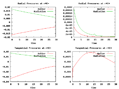
As it can be appreciated from figure 3, it is found that the hydrodynamic & radiation pressures become of same order of magnitude and at the core, radiation pressure is larger. This is consistent with the picture we expect for the radiation hydrodynamics within a general relativistic gravitational collapse [28]. Figure (3) shows how the shock front bounces, from a collapsing core it turns to expand violently.

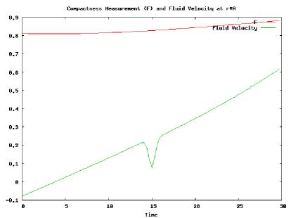
The shock strength, $N$, also appears to be a very significant feature concerning the evolution of the distribution, because it drastically increases the fluid velocity behind the shock. From equation (22) we undertand that this parameter cannot to be less than one because it leads to imaginary speed of the shock. The reason is that the fraction When we raise the shock force parameter, the fluid velocity increases faster to relativistic values and even for certain critical value (it depends on the whole set of initial conditions) it reaches light speed rapidly.

As we have stressed, these are preliminary results that should deserve further simulations.

References

- [1] Bruenn, SW, De Nisco, KR, and Mezzacappa, A (2001) Astrophys J., 560, 326. (Preprint: astro-ph 0101400)
- [2] Bower, R and Liang, EP (1974), Astrophys. J., 188, 657.
- [3] Herrera, L and Santos NO (1997), Physics Reports, 286, 53.
- [4] Herrera, L, Martín J and Ospino J (2002) J. Math. Phys. 43, 4889. (Preprint: gr-qc 0207040)
- [5] Herrera,L, DiPrisco, A, Martin, J, Ospino, J, Santos, NO and Troconis, O (2004) Phys. Rev. D 69, 84026. (Preprint: gr-qc 0403006.
- [6] Chaisi, M and Maharaj, SD (2005) Gen. Rel. Grav. 37 1177. (Preprint: gr-qc 0504098)
- [7] Chaisi, M and Maharaj, SD (2006) Pramana - J. Phys. 37 609. (Preprint: gr-qc 0504098)
- [8] Dev, K and Gleiser, M (2002) Gen. Relativ. Gravit. 34, 1793.
- [9] Dev, K and Gleiser, M (2003) Gen. Relativ. Gravit. 35, 1435. (Preprint: gr-qc 0303077)
- [10] Ivanov, BV (2002) Phys. Rev. D 65, 10411. (Preprint: gr-qc 0203070)
- [11] Mak, MK and Harko, T (2002) Chin. J. Astron. Astrophys. 2, 248.
- [12] Mak, MK and Harko, T (2003) Proc. Roy. Soc. Lond. A 459, 393 (Preprint: gr-qc 0110103).
- [13] Sharma, R and Mukherjee, S (2002) Mod. Phys. Lett. A 17, 2535.
- [14] Font, J (2003) “Numerical Hydrodynamics in General Relativity”, Living Rev. Relativity 6, 4. On line article: http://www.livingreviews.org/lrr-2003-4/ ( (Preprint: gr-qc 0003101)
- [15] The code GR Astro and its documentation can be found at http://wugrav.wustl.edu/Codes/GR3D Also see CACTUS http://www.cactuscode.org
- [16] Herrera, L, Jiménez, J and Ruggeri, G (1980) Phys. Rev. D22, 2305.
- [17] Barreto,W, Martínez, H and Rodríguez B (2002) Ap. Space Sc. 282 581 (Preprint: gr-qc 0211033)
- [18] Herrera L, Barreto W, Di Prisco A, and Santos NO (2002) Phys. Rev. D65, 104004. (Preprint: gr-qc 0202051)
- [19] Herrera, L, DiPrisco A and Barreto, W (2006) Phys.Rev. D 73, 024008 (Preprint: gr-qc 0512032)
- [20] Domínguez Cascante, R (1997) Jour. of Phys A, 30 7707 (Preprint: cond-mat 9709104)
- [21] Pons, JA, Ibañez, JMa and Miralles JA (2000) Mon. Not. R. Astr. Soc, 317, 550 (Preprint: astro-ph 0005310)
- [22] Smit, JM, Van den Horn, LJ and Bludman, SA (2000) Astron. Astrophys. 356, 559.
- [23] Aguirre, F, Núñez, LA and Soldovieri T (2005) Variable Eddington Factor and Radiating Slowly Rotating Bodies in General Relativity. Preprint gr-qc 0503085.
- [24] Herrera, L and Núñez, LA (1990) Fund. Cosmic Phys. 14, 235.
- [25] Herrera, L and Núñez, LA (1987), Astrophys. J., 319: 868.
- [26] Herrera L and Núñez L (1989) Astrophys. J., 339 339.
- [27] Herrera, L, Barreto, W and Núñez LA (1991) Astrophys. J., 375, 663.
- [28] Mihalas, D and Weibel Mihalas, B (1984) Foundations of Radiation Hydrodynamics (Oxford University Press).
- [29] Cosenza, M, Herrera, L, Esculpi, M and Witten, L (1980) J. Math. Phys., 22, 118.
- [30] Bonnor, WB and Vickers, PA (1981) Gen. Relativ. Gravit. 13, 29.
- [31] Taub, AH (1948) Phys. Rev. 74, 328.