Inside the BTZ black hole

Abstract

We consider static circularly symmetric solution of three-dimensional Einstein’s equations with negative cosmological constant (the BTZ black hole). The case of zero cosmological constant corresponding to the interior region of a black hole is analyzed in detail. We prove that the maximally extended BTZ solution with zero cosmological constant coincides with flat three-dimensional Minkowskian space-time without any singularity and horizons. The Euclidean version of this solution is shown to have physical interpretation in the geometric theory of defects in solids describing combined wedge and screw dislocations.

1 Introduction

Three-dimensional static circularly symmetric solution of three-dimensional Einstein’s equations (the BTZ black hole [1]) attracted much interest last years, and is believed to be a good relatively simple laboratory for analyzing general aspects of black hole physics. The BTZ solution is the most general black hole solution in three dimensions, which is guaranteed by the three-dimensional version of Birkhoff’s theorem [2]. It has very interesting classical and quantum properties (for review see, i.e. [3]).

Global structure of the BTZ solution was analyzed in [4, 5]. In these articles the black hole space-time was considered as the quotient space of the anti-de Sitter space by the action of the discrete transformation group. This approach deserves a deeper analysis because the transformation group has fixed points, and therefore the quotient space is not a manifold. The situation is unclear especially in the interior region of the black hole. To clarify the global structure of the interior region, we consider the BTZ solution for zero cosmological constant. In this simple case, all coordinate transformations can be written explicitly, and behavior of geodesics is analyzed. We prove that the maximally extended (along geodesics) BTZ solution for zero cosmological constant coincides with flat Minkowskian space-time without any singularity and horizons for infinite range of the angle coordinate $\varphi$. The BTZ solution in the original coordinates covers only one half of the Minkowskian space-time, and the two planes corresponding to $r=0$ are just coordinate singularities. Two copies of the BTZ solution cover the whole Minkowskian space-time and are smoothly glued at $r=0$.

If we make the angle identification $\varphi\sim\varphi+2\pi$ than four cones with the same vertex appear in the interior region of the BTZ black hole located at the inner horizon $r_{-}$.

Next we analyze the Euclidean version of the BTZ solution. In this case the solution has physical interpretation in solid state physics. In the geometric theory of defects developed in [6, 7, 8, 9] (for review see [10]) it depends on the Poisson ratio and describes combined wedge and screw dislocations.

2 The BTZ solution

We consider a three-dimensional manifold ${\mathbb{M}}$ with local coordinates $x^{\mu}$, $\mu=0,1,2$. Suppose it is endowed with a Lorentzian signature metric $g_{\mu\nu}(x)$, ${\sf\,sign\,}g_{\mu\nu}=(+--)$, which satisfies Einstein’s equations

$$R_{\mu\nu}=\Lambda g_{\mu\nu}$$ (1)

with a cosmological constant $\Lambda=-2/l^{2}$. In three dimensions the full curvature tensor is defined by its Ricci tensor

$$R_{\mu\nu\rho\sigma}=-\varepsilon_{\mu\nu\lambda}\varepsilon_{\rho\sigma\zeta}R^{\lambda\zeta},~{}~{}~{}~{}R_{\mu\nu}=R_{\mu\rho\nu}{}^{\rho}$$

where $\epsilon_{\mu\nu\lambda}$ is the totally antisymmetric tensor, $\epsilon_{012}=\sqrt{\det g_{\mu\nu}}$. Therefore, any smooth solution of Einstein’s equations on a manifold (by solution we mean a pair $({\mathbb{M}},g)$) is a space-time of constant curvature. The universal covering spaces for positive, zero, and negative cosmological constant are respectively de Sitter, Euclidean, and anti de Sitter spaces. All other smooth solutions $({\mathbb{M}},g)$ are obtained from these solutions by an action of an isometry transformation group which acts freely and properly discontinuous (see, i.e. [11]). Afterwards, a solution will be isometric to some fundamental domain of de Sitter, Euclidean, or anti de Sitter space with properly identified boundaries. These solutions are considered as known ones though explicit action of a transformation group may be quite complicated. All these solutions are smooth, have no singularities and horizons, and therefore do not describe black holes.

Theory becomes much richer if we admit the existence of singularities at points, lines, or surfaces in ${\mathbb{M}}$. The famous BTZ solution is [1]

$$\begin{split}ds^{2}&=\left(-M+\frac{J^{2}}{4r^{2}}+\frac{r^{2}}{l^{2}}\right)dt^{2}-\frac{dr^{2}}{\left(-M+\frac{J^{2}}{4r^{2}}+\frac{r^{2}}{l^{2}}\right)}-r^{2}\left(d\varphi-\frac{J}{2r^{2}}dt\right)^{2},\\ &=\left(-M+\frac{r^{2}}{l^{2}}\right)dt^{2}-\frac{dr^{2}}{\left(-M+\frac{J^{2}}{4r^{2}}+\frac{r^{2}}{l^{2}}\right)}-r^{2}d\varphi^{2}+Jdtd\varphi,\end{split}$$ (2)

where $M$ and $J$ are two integration constants, having physical interpretation of the mass and angular momentum of the black hole. We shall see later that the inner horizon $r_{-}$ becomes a line in ${\mathbb{M}}$ with four cones at each point. This solution is supposed to be written in cylindrical coordinate system

$$t\in(-\infty,\infty),~{}~{}r\in(0,\infty),~{}~{}\varphi\in(0,2\pi).$$ (3)

Metric (2) has two commuting Killing vector fields: $K_{1}=\partial_{t}$ and $K_{2}=\partial_{\varphi}$.

Outer $r_{+}$ and inner $r_{-}$ horizons of the BTZ solution

$$r^{2}_{\pm}=\frac{Ml^{2}}{2}\left(1\pm\sqrt{1-\frac{J^{2}}{M^{2}l^{2}}}\right)$$

are defined by two positive zeroes of the function

$$N(r)=-M+\frac{J^{2}}{4r^{2}}+\frac{r^{2}}{l^{2}}=0.$$

Here we assume that $|J|<Ml$.

We make four comments on the form of this solution.

1) The space-time $(M,g)$ with metric (2), (3) is not locally a constant curvature space, because any point lying in the singularity $r=r_{-}$ do not have a neighborhood of constant curvature. Here we consider singular points $(t,r=r_{-},\varphi)$ belonging to ${\mathbb{M}}$. In fact, we shall see that points $r=r_{-}$ are not points of a manifold, and do not have neighborhoods diffeomorphic to a ball at all.

2) The range of $\varphi$ is determined by its interpretation as an angle in the region $r\to\infty$ where the space-time becomes asymptotically anti-de Sitter. The mass is supposed to be positive, because otherwise there is no horizon. The case $M<0$ and $\Lambda>0$, corresponding to de Sitter asymptotic (which has a horizon) is not considered because $\varphi$ can not be interpreted as the angle coordinate in this case. The sign of $J$ corresponds to left and right rotations and does not contribute to the global structure of the solution. Thus, range of coordinates (3) and the signs of the cosmological constant and the mass are uniquely determined by two requirements: (i) $\varphi$ is an angle in the asymptotic region $r\to\infty$ and (ii) the solution has at least one horizon.

3) For zero cosmological constant $\Lambda=0$ and angular momentum $J=0$ the metric is

$$ds^{2}=-Mdt^{2}+\frac{dr^{2}}{M}-r^{2}d\varphi^{2}.$$

For positive mass $M>0$, it has no conical singularity at $r=0$ because now $r$ and $\varphi$ are coordinates on the two-dimensional Minkowskian space-time of signature $(+-)$ but not on the Euclidean plane. This is in contrast with a common belief that static point particles in three-dimensional gravity are described by conical singularities, distributed on a space-like section of ${\mathbb{M}}$ [12, 13, 14].

4) There are four regions of $r$ where coordinate lines $t,r$, and $\varphi$ have different types of tangent vectors. Coordinate lines $t$ and $r$ may be either timelike or spacelike, depending on range of $r$ which has three distinguished points: $r_{+},r_{-}$, and $r_{3}=Ml^{2}$. The coordinate line $\varphi$ is always spacelike. We summarize different properties of coordinates in the Table, where plus and minus signs denote respectively timelike and spacelike character of coordinates.

	$t$	$r$	$\varphi$
$r_{3}<r<\infty$	$+$	$-$	$-$
$r_{+}<r<r_{3}$	$-$	$-$	$-$
$r_{-}<r<r_{+}$	$-$	$+$	$-$
$0<r<r_{-}$	$-$	$-$	$-$

Table 1: Timelike “$+$” and spacelike “$-$” character of coordinate lines in different regions of $r$.

We see that the coordinate $t$ is timelike only for large $r>r_{3}$. In two regions, $r_{+}<r<r_{3}$ and $0<r<r_{-}$, all coordinates are spacelike.

Global structure of solution (2) was described in [4] in terms of the quotient space of the anti-de Sitter space, and the Carter–Penrose diagrams were drawn for the metric

$$dl^{2}=Ndt^{2}-N^{-1}dr^{2}.$$ (4)

This description deserves a deeper analysis especially at the vicinity of the singularity for two reasons. First, the transformation group used to obtain the quotient of the anti-de Sitter space in [4] does not act freely because it has fixed points [5]. Second, the coordinate lines have different character, and the induced metric on sections of ${\mathbb{M}}$ corresponding to constant angle $\varphi={\sf\,const}$ differs essentially from (4). Therefore we can not say that the global solution is topologically the product of the Carter–Penrose diagram on a circle. In the next section we give a different description of the global structure in terms of the product of real line $t^{\prime}\in{\mathbb{R}}$ on the corresponding Carter–Penrose diagram.

3 The interior region of the BTZ black hole

By global solution we mean a pair $({\mathbb{M}},g)$ where (i) the metric satisfies Einstein’s equations and (ii) any extremal (geodesic) either can be continued in both directions to an infinite value of the canonical parameter or it ends up at a singular point at a finite value. This solution is also called maximally extended. To construct a maximally extended solution for BTZ metric (2) we shall use a conformal block method described in [15] which was developed for two-dimensional metrics having one Killing vector field.

To analyze global structure of the interior region of the BTZ black hole, we assume that cosmological constant is zero, $\Lambda=0$ or $l\to\infty$. This assumption simplifies essentially formulae, which now may be written explicitly. Moreover, in this case the solution has direct interpretation in the geometric theory of defects describing a linear dislocation which is a combination of screw and wedge dislocations (see section 5).

For later comparison, we draw the Carter–Penrose diagram for two-dimensional metric (4) with

$$N(r)=-\alpha^{2}+\frac{c^{2}}{r^{2}},$$ (5)

where for simplicity we introduced new notations $M=\alpha^{2}$ and $c=J/2$. In the geometric theory of defects, $\alpha=1+\theta$, where $\theta$ is the deficit angle of the wedge dislocation, and $c=b/2\pi$, where $b$ is the Burgers vector of the screw dislocation. The function (5) becomes a conformal factor in coordinates $t,r^{\prime}$ where new radial coordinate $r^{\prime}$ is determined by the ordinary differential equation

$$\frac{dr}{dr^{\prime}}=N(r).$$

In these coordinates, the global structure is easily analyzed [15], and the Carter–Penrose diagram for the surface with metric (4), (5) is shown in Fig. 1

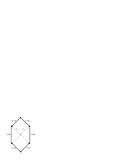
Figure 1: The Carter–Penrose diagram corresponding to a surface with metric (4), (5). Solid lines denote complete null infinity. The timelike boundary $r=0$ is incomplete, and the two-dimensional curvature is singular here. Filled circles denote complete space and time infinities.

It has one horizon at $r_{-}$. In the limit $l\to\infty$ the outer horizon $r_{+}$ moves to infinity and the boundary $r=\infty$ becomes geodesically complete which is shown by solid thick lines. At the boundaries $r=0$, the two dimensional curvature for metric (4), (5) is singular. Filled circles denote complete future, past and right, left “infinities”. A circle in the center denotes incomplete vertex of conformal blocks. Unfortunately, the induced metric on sections of ${\mathbb{M}}$ corresponding to $\varphi={\sf\,const}$

$$dl^{2}=-\alpha^{2}dt^{2}-\frac{dr^{2}}{-\alpha^{2}+\frac{c^{2}}{r^{2}}}$$

is quite different from (4), (5). This metric is degenerate at the horizon $r_{-}=c/\alpha$, where it changes signature. Therefore, we are not able to draw at least one Carter–Penrose diagram for it.

To avoid this difficulty, we draw the Carter–Penrose diagram for sections of constant “time” which is a spacelike coordinate inside the BTZ black hole. First, we diagonalize the metric on ${\mathbb{M}}$

$$ds^{2}=-\alpha^{2}dt^{2}-\frac{dr^{2}}{-\alpha^{2}+\frac{c^{2}}{r^{2}}}-r^{2}d\varphi^{2}+2cd\varphi dt.$$ (6)

Performing the linear nondegenerate coordinate transformation

$$t=t^{\prime}+\frac{c}{\alpha^{2}}\varphi,$$ (7)

and keeping coordinates $r$ and $\varphi$ untouched, we obtain

$$ds^{2}=-\alpha^{2}dt^{\prime 2}-\frac{dr^{2}}{-\alpha^{2}+\frac{c^{2}}{r^{2}}}-\left(r^{2}-\frac{c^{2}}{\alpha^{2}}\right)d\varphi^{2}.$$ (8)

Now the three-dimensional space-time can be represented as a product ${\mathbb{M}}={\mathbb{R}}\times{\mathbb{U}}$ where $t^{\prime}\in{\mathbb{R}}$ and $(r,\varphi)\in{\mathbb{U}}$. The two-dimensional surface ${\mathbb{U}}$ (sections of ${\mathbb{M}}$ corresponding to $t^{\prime}={\sf\,const}$) possesses the induced metric of Lorentzian signature. At this point we assume that $\varphi\in{\mathbb{R}}$ making the identification $\varphi\sim\varphi+2\pi$ afterwards. Changing the radial coordinate,

$$r=\sqrt{2\alpha\sigma},~{}~{}~{}~{}\sigma>0~{}~{}\text{for}~{}~{}\alpha>0,$$ (9)

the induced metric on ${\mathbb{U}}$ becomes

$$dl^{2}=-\frac{\alpha^{2}d\sigma^{2}}{c^{2}-2\alpha^{3}\sigma}+\frac{c^{2}-2\alpha^{3}\sigma}{\alpha^{2}}d\varphi^{2}.$$ (10)

The conformal factor for the induced metric $N(\sigma)=(c^{2}-2\alpha^{3}\sigma)/\alpha^{2}$ is a linear function of $\sigma$ and therefore describes a surface of zero two-dimensional curvature. It has one horizon at $\sigma_{-}=c^{2}/2\alpha^{3}$ corresponding to inner horizon $r_{-}$. The maximally extended surfaces $(\sigma,\varphi)\in{\mathbb{U}}$ is represented by the Carter–Penrose diagram in Fig. 2.

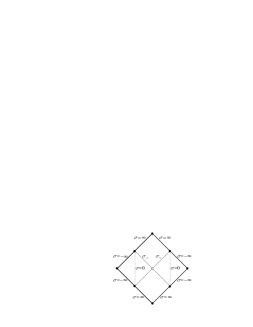
Figure 2: The Carter–Penrose diagram corresponding to the surface ${\mathbb{U}}$ with metric (10). It represents two-dimensional flat Minkowskian plane in $\sigma,\varphi$ coordinates. The boundary is complete. Two copies of the BTZ solution are smoothly glued together along timelike dashed lines $\sigma=0$.

Here the maximal extension requires the infinite range of coordinates $\sigma\in{\mathbb{R}}$ and $\varphi\in{\mathbb{R}}$. To consolidate this range of coordinates with the original radial coordinate (9) we assume that $\sigma>0$ for $\alpha>0$ and $\sigma<0$ for $\alpha<0$, and make the identification $(\sigma,\alpha)\sim(-\sigma,-\alpha)$. We see that after the identification we must consider two-dimensional surfaces $r=0$ for ${\mathbb{M}}$ as the boundary.

3.1 Geodesics

The behavior of geodesics for the BTZ solution was considered in [16, 17]. In the case of zero cosmological constant equations for geodesics are greatly simplified, and a general solution can be written in elementary functions and analyzed in detail.

To understand the nature of the singularity at $r_{-}$ we analyze the behavior of geodesics $x^{\mu}(\tau)=\left(\vphantom{\frac{a}{b}}t(\tau),r(\tau),\varphi(\tau)\right)$ for metric (6) in this section. The only nonzero Christoffel’s symbols are

$$\Gamma_{11}{}^{1} =-\frac{c^{2}}{r(\alpha^{2}r^{2}-c^{2})}, \qquad\Gamma_{12}{}^{0}=\Gamma_{21}{}^{0} =\frac{cr}{\alpha^{2}r^{2}-c^{2}},$$

$$\Gamma_{22}{}^{1} =\frac{\alpha^{2}r^{2}-c^{2}}{r}, \qquad\Gamma_{12}{}^{2}=\Gamma_{21}{}^{2} =\frac{\alpha^{2}r}{\alpha^{2}r^{2}-c^{2}}.$$

The equations for geodesics

$$\ddot{x}^{\mu}=-\Gamma_{\nu\rho}{}^{\mu}\dot{x}^{\nu}\dot{x}^{\rho},$$ (11)

where dots denote differentiation with respect to the canonical parameter $\tau$, become

$$\begin{split}\ddot{t}&=-2\frac{cr}{\alpha^{2}r^{2}-c^{2}}\dot{r}\dot{\varphi},\\ \ddot{r}&=\frac{c^{2}}{r(\alpha^{2}r^{2}-c^{2})}\dot{r}^{2}-\frac{\alpha^{2}r^{2}-c^{2}}{r}\dot{\varphi}^{2},\\ \ddot{\varphi}&=-2\frac{\alpha^{2}r}{\alpha^{2}r^{2}-c^{2}}\dot{r}\dot{\varphi}.\end{split}$$ (12)

These equations can be integrated in elementary functions. First, we note that any system of equations for geodesics has a conserved quantity: the length of a tangent vector $C_{0}=g_{\mu\nu}\dot{x}^{\mu}\dot{x}^{\nu}$. It corresponds to conservation of energy of a point particle which, by assumption, moves along a geodesic line

$$C_{0}=-\alpha^{2}\dot{t}^{2}+\frac{r^{2}}{\alpha^{2}r^{2}-c^{2}}\dot{r}^{2}-r^{2}\dot{\varphi}^{2}+2c\dot{t}\dot{\varphi}.$$ (13)

Another two conservations laws $C_{1,2}=g_{\mu\nu}\dot{x}^{\mu}K_{1,2}^{\nu}$ correspond to the symmetry of the metric, generated by two Killing vector fields: $K_{1}=\partial_{t}$ and $K_{2}=\partial_{\varphi}$. They describe respectively conservation of momenta and angular momenta

$$C_{1} =-\alpha^{2}\dot{t}+c\dot{\varphi},$$ (14)

$$C_{2} =~{}~{}c\dot{t}-r^{2}\dot{\varphi}.$$ (15)

Conservation laws (13)–(15) can be easily solved with respect to the first derivatives

$$\begin{split}\dot{t}&=-\frac{r^{2}C_{1}+cC_{2}}{\alpha^{2}r^{2}-c^{2}},\\ \dot{r}^{2}&=\frac{\alpha^{2}r^{2}-c^{2}}{r^{2}}C_{0}+\frac{r^{2}C_{1}^{2}+2cC_{1}C_{2}+\alpha^{2}C_{2}^{2}}{r^{2}},\\ \dot{\varphi}&=-\frac{cC_{1}+\alpha^{2}C_{2}}{\alpha^{2}r^{2}-c^{2}}.\end{split}$$ (16)

These equations are compared with their Euclidean counterpart in section 4.2. We show that the connected Lorentzian manifold breaks into disconnected pieces along horizons in the Euclidean case.

Equations for geodesics (16) can be integrated explicitly. To make clear further integration we perform the transformation to Cartesian coordinates.

3.2 Transformation to Cartesian coordinates

In this section we perform the coordinate transformation which brings the metric (8) into the usual Lorentzian form and shows that the Carter–Penrose diagram in Fig.2 represents the Minkowskian plane. We consider three-dimensional Minkowskian space ${\mathbb{R}}^{1,2}$ with the Lorentz metric in Cartesian coordinates

$$ds^{2}=dT^{2}-dX^{2}-dY^{2}.$$ (17)

We introduce polar coordinates $0<R<\infty,-\infty<\Phi<\infty$ in each of the four quadrants in the $T,X$ plane (see Fig.3)

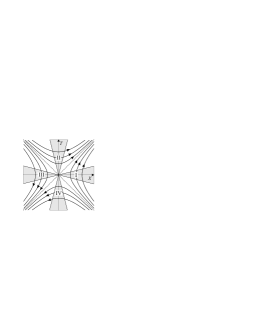
Figure 3: Polar coordinates in the Minkowskian plane. Solid lines are hyperbolas of constant $R$. Arrows show increasing of the angle $\Phi$. Shadowed regions denote the fundamental domain of the transformation group $\Phi\rightarrow\Phi+2\pi\alpha$.

$$\begin{split}\text{I}:~{}~{}&T=~{}~{}R\sinh\Phi,\\ &X=~{}~{}R\cosh\Phi,\\ \text{III}:~{}~{}&T=-R\sinh\Phi,\\ &X=-R\cosh\Phi,\end{split}\qquad\begin{split}\text{II}:~{}~{}&T=~{}~{}R\cosh\Phi,\\ &X=~{}~{}R\sinh\Phi,\\ \text{IV}:~{}~{}&T=-R\cosh\Phi,\\ &X=-R\sinh\Phi.\end{split}$$

This transformation is degenerate on two lines $R=0$, and metric on the $T,X$ plane becomes

$$\begin{split}\text{I,III}:\quad dl^{2}&=-dR^{2}+R^{2}d\Phi^{2},\\ \text{II,IV}:\quad dl^{2}&=dR^{2}-R^{2}d\Phi^{2}.\end{split}$$ (18)

Performing the further transformation

$$\text{I,III}:\quad R =\frac{\sqrt{c^{2}-2\alpha^{3}\sigma}}{\alpha^{2}}, \quad\sigma <\frac{c^{2}}{2\alpha^{3}}$$

$$\text{II,IV}:\quad R =\frac{\sqrt{2\alpha^{3}\sigma-c^{2}}}{\alpha^{2}}, \quad\sigma >\frac{c^{2}}{2\alpha^{3}}$$

$$\text{I--IV}:\quad \Phi =\alpha\varphi, \quad-\infty <\varphi<\infty,$$

$$Y =\alpha t^{\prime}, -\infty <t^{\prime}<\infty,$$

we arrive precisely to metric (8), (10).

Now integrating equations (11) for geodesics becomes trivial. A general solution is

$$\begin{split}T&=t_{0}+v_{0}\tau,\\ X&=x_{0}+v_{1}\tau,\\ Y&=y_{0}+v_{2}\tau,\end{split}$$

and depends on six arbitrary constants: a position of a point in the Minkowskian space $t_{0},x_{0},y_{0}$ and a velocity $v_{0},v_{1},v_{2}$ of the geodesic which goes through this point. The inverse transformation, for example, in the first quadrant is

$$\begin{split}t&=\frac{1}{\alpha}\left[Y+\frac{c}{\alpha^{2}}{\sf\,arcth\,}\left(\frac{T}{X}\right)\right],\\ r&=\frac{1}{\alpha}\sqrt{c^{2}-\alpha^{4}(X^{2}-T^{2})},\\ \varphi&=\frac{1}{\alpha}{\sf\,arcth\,}\left(\frac{T}{X}\right).\end{split}$$

Elementary analysis shows that constants of integration (13)–(15) are

$$\begin{split}C_{0}&=v_{0}^{2}-v_{1}^{2}-v_{2}^{2},\\ C_{1}&=-\alpha v_{2},\\ C_{2}&=\frac{cv_{2}}{\alpha}+\alpha(x_{0}v_{0}-t_{0}v_{1}).\end{split}$$

The considered coordinate transformations prove that the Carter–Penrose diagram in Fig.2 represents a Minkowskian plane ${\mathbb{R}}^{1,1}$. The global BTZ solution with zero cosmological constant is thus a product ${\mathbb{R}}\times{\mathbb{R}}^{1,1}={\mathbb{R}}^{1,2}$, i.e. a flat three-dimensional Minkowskian space-time.

Now the maximally extended BTZ solution with zero cosmological constant (6) and infinite range of $\varphi$ becomes transparent: it is a flat three-dimensional Minkowskian space-time ${\mathbb{R}}^{1,2}$ without any singularity and horizons. BTZ solution (6) covers only one half of it. Maximal extension means that the BTZ solution for $0<\sigma<\infty$ is prolonged to negative values $-\infty<\sigma<\infty$. For negative $\sigma$ we can define new coordinate $r=\sqrt{2\alpha\sigma}$, $\sigma<0$ and $\alpha<0$ and again arrive at the BTZ solution. Thus, two copies of BTZ solution cover the whole Minkowskian space-time ${\mathbb{R}}^{1,2}$ and are smoothly glued together at $r=0$. The “singularity” at $r=0$ is a purely coordinate one which is clear from the transformation (9). We stress that the above analysis was performed for the whole range of the angle $\varphi\in{\mathbb{R}}$. The periodicity of the angle will be considered in the next section.

3.3 Periodicity of $\varphi$

Having in mind that the coordinate $\varphi$ is interpreted as the angle $0<\varphi<2\pi$ in the exterior region of the BTZ solution with negative cosmological constant, we assume that the identification $\varphi\sim\varphi+2\pi$ takes also place for zero cosmological constant. The transformation group ${\mathbb{G}}:~{}\varphi\rightarrow\varphi+2\pi$ acts freely and properly discontinuous on a line $\varphi\in{\mathbb{R}}$ but not in the Minkowskian space-time ${\mathbb{R}}^{1,2}$. In the last case it has fixed points and the quotient space ${\mathbb{R}}^{1,2}/{\mathbb{G}}$ itself is not a manifold.

Periodicity in $\varphi$ means periodicity in the polar angle $\Phi\sim\Phi+2\pi\alpha$ in the Minkowskian plane $T,X$ considered in the previous section. The transformation group identifies points along hyperbolas $R={\sf\,const}$ corresponding to different polar angles $\Phi\sim\Phi+2\pi\alpha$. Its action is not defined on two lines $R=0$ where polar coordinates are degenerate. Considering these lines as the limit of hyperbolas, we assume that all their points are mapped into the origin under the action of the transformation group ${\mathbb{G}}$. Then the transformation group acting in the $T,X$ plane has the fundamental domain consisting of four wedges with identified boundaries shown by shadowed regions in Fig. 3. We denote them by I-IV according to the number of the corresponding quadrant. Identifying boundaries of the wedge makes it a cone. The vertexes of cones are glued in the origin of the Cartesian coordinate system. The origin is a fixed point for the transformation group and not a point of a manifold. Indeed, it does not have a neighborhood diffeomorphic to a disc. At the same time, it can not be excluded from the space-time because it lies at a finite distance. Thus, we have four cones in the Minkowskian plane with the common vertex in the origin. They are not conical singularities because the plane is equipped with the Lorentzian signature metric.

The Killing vector $K_{2}=\partial_{\varphi}=\alpha\partial_{\Phi}$ of the whole three-dimensional metric (6) is also the Killing vector for two-dimensional metric (18). Hence, the transformation group ${\mathbb{G}}$ is the isometry for two-dimensional Minkowskian plane $T,X$.

The identification $\varphi\sim\varphi+2\pi$ acts also nontrivially on the third “time” coordinate $t^{\prime}$ in (7), but it remains well defined.

Now we analyze the behavior of geodesics in the $T,X$ plane. They are clearly straight lines before the identification. Let us fix an arbitrary fundamental domain $(\Phi_{0},\Phi_{0}+2\pi\alpha)$ and a timelike geodesic $1$, shown in Fig. 4. Particle moving along geodesic 1 in the $T,X$ plane wraps around a cone. Its trajectory is represented by the sequence of segments of straight lines in the fundamental domain, each segment representing one rotation around the cone. The equation of geodesic 1 in polar coordinates in the first quadrant is

$$R=R_{0}\frac{\tan\gamma_{1}\cosh\Phi_{0}-\sinh\Phi_{0}}{\tan\gamma_{1}\cosh\Phi-\sinh\Phi},$$

where $\gamma_{1}$ is the inclination of the line $1$. Its segment from $R_{0}$ to

$$R_{1}=R_{0}\frac{\tan\gamma_{1}\cosh\Phi_{0}-\sinh\Phi_{0}}{\tan\gamma_{1}\cosh(\Phi+2\pi\alpha)-\sinh(\Phi_{0}+2\pi\alpha)}$$

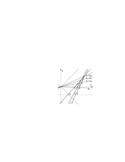
Figure 4: The image of the geodesic $1$ in the fundamental domain $\Phi_{0},\Phi_{0}+2\pi\alpha$. It consists of segments of straight lines with inclinations $\gamma_{1},\gamma_{2},\gamma_{3},\dotsc$ which cross the line $\Phi_{0}$ respectively at points $R_{0},R_{1},R_{2},\dotsc$.

belongs to the fundamental domain. The next segment corresponding to polar angle $\Phi\in(\Phi_{0}+2\pi\alpha,\Phi_{0}+4\pi\alpha)$ is identified with the segment of line $2$ lying in the fundamental domain $(\Phi_{0},\Phi_{0}+2\pi\alpha)$ but having different inclination $\gamma_{2}$. Continuing this procedure, we obtain equation for the $k$-th line

$$R=R_{k-1}\frac{\tan\gamma_{k}\cosh\Phi_{0}-\sinh\Phi_{0}}{\tan\gamma_{k}\cosh\Phi-\sinh\Phi},$$

where

$$R_{k}=R_{0}\frac{\tan\gamma_{1}\cosh\Phi_{0}-\sinh\Phi_{0}}{\tan\gamma_{1}\cosh(\Phi_{0}+\alpha_{k})-\sinh(\Phi_{0}+\alpha_{k})},$$ (19)

and we introduced shorthand notation

$$\alpha_{k}=2\pi\alpha k,~{}~{}~{}~{}k=0,\pm 1,\pm 2,\dotsc.$$

On the other hand, the segment of line $k$ in the fundamental domain can be obtained as the projection of the segment of the previous line $k-1$

$$R_{k}=R_{k-1}\frac{\tan\gamma_{k}\cosh\Phi_{0}-\sinh\Phi_{0}}{\tan\gamma_{k}\cosh(\Phi_{0}+\alpha_{1})-\sinh(\Phi_{0}+\alpha_{1})}.$$ (20)

Comparing Eqs. (19) and (20), we express the inclination angle $\gamma_{k}$ of the $k$-th line through the original inclination angle $\gamma_{1}$

$$\tan\gamma_{k}=\frac{\tan\gamma_{1}-\tanh\alpha_{k-1}}{1-\tan\gamma_{1}\tanh\alpha_{k-1}}.$$ (21)

It is important that the inclination angles of segments depend only on the original inclination angle $\gamma_{1}$. They do not depend on the fundamental domain characterized by the angle $\Phi_{0}$ and the distance from the origin $R_{0}$.

Equation (21) is also valid for lightlike and spacelike geodesics.

As the consequence of Eq.(21), we see that segments of all lightlike geodesics $\tan\gamma_{1}=\pm 1$ remain lightlike $\tan\gamma_{k}=\pm 1$. All segments for timelike and spacelike geodesics are respectively timelike and spacelike having the same limit

$$\lim_{k\to\pm\infty}\tan\gamma_{k}=\mp 1.$$

We see also that there are no closed timelike geodesics.

To get a deeper insight into the behavior of geodesics we consider $\alpha_{k}$ as a continuous variable

$$\tan\gamma_{\alpha}=\frac{\tan\gamma_{1}-\tanh\alpha}{1-\tan\gamma_{1}\tanh\alpha}.$$

This function is plotted in Fig.5. For timelike geodesics $|\tan\gamma_{1}|>1$ it is singular when

$$\tanh\alpha\tan\gamma_{1}=1$$ (22)

and has two branches.

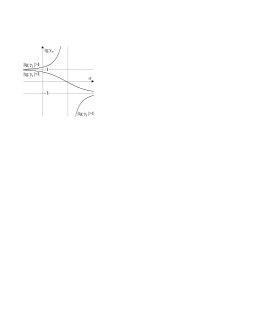
Figure 5: The inclination of the trajectory segment versus continuous parameter $\alpha_{k}\rightarrow\alpha$. For timelike geodesics $|\tan\gamma_{1}|>1$, it has two branches with the singularity at $\tanh\alpha\tan\gamma_{1}=1$, corresponding to the turning point. The dependence is smooth for spacelike geodesics $|\tan\gamma_{1}|<1$.

The upper and lower branches correspond to the motion of a particle respectively to the right and left in the first quadrant, the singularity (22) being the turning point.

All timelike geodesics start and end at the origin of the Cartesian coordinate system at finite values of proper time parameter making infinite number of rotations around the cone. Spacelike geodesics which do not lie entirely in one fundamental region approach the origin on the left making infinite number of rotations at a finite value of canonical parameter and go to the right space infinity.

To understand the behavior of geodesics in other quadrants, it is sufficient to rotate the picture on ninety degrees.

The behavior of geodesics at the origin of Cartesian coordinates is not defined. It can be naturally done by unfolding the cones and going back to Minkowskian plane $T,X$. Then timelike geodesics which do not cross boundary of the fundamental region IV are continued to the fundamental region II. Those timelike geodesics which cross the boundary of the fundamental region IV are continued to the fundamental domain I or III depending on the inclination. In the region I they move to the right at a finite distance, then return back to the origin, and are continued to the fundamental domain II. We draw trajectory of a static particle in the $T,X$ plane after the identification in Fig.6.

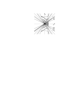
Figure 6: The trajectory of a static particle in the $T,X$ plane. The fundamental domain is chosen symmetrically $(-\pi,\pi)$ in each quadrant. After the identification $\varphi\sim\varphi+2\pi$ it makes infinite number of rotations around the cone in the fourth quadrant at a finite proper time. Afterwards it moves to the right in the first quadrant, returns back, making also an infinite number of rotations near the cone vertex, and goes to the second quadrant. There, after an infinite number of rotations, it goes to infinity.

Timelike curves $R={\sf\,const}$ (which are not geodesics) are closed loops after the identification $\Phi\sim\Phi+2\pi\alpha$. Thus, any particle with constant acceleration (in terms of Cartesian coordinates) has a closed timelike world line at regions I,III.

To conclude this section, we draw the Carter–Penrose diagram for the Minkowskian plane after the polar angle identification $\Phi\sim\Phi+2\pi\alpha$ in Fig.7. It looks like a flower.

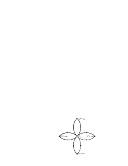
Figure 7: The Carter–Penrose diagram for the Minkowskian plane after the polar angle identification $\Phi\sim\Phi+2\pi\alpha$.

4 Euclidean version of the interior of the BTZ solution

The Euclidean version of the BTZ solution was considered in [18] when analyzing its thermodynamical properties. In this section we analyze global structure and geodesics of the Euclidean BTZ solution for zero cosmological constant.

Here, we use many notations from the previous section though their meaning in the Euclidean case is often different. We hope that this step does not cause any inconvenience and simplifies the comparison of the two cases.

The Euclidean counterpart of the BTZ metric (2) is given by the transformation $r\rightarrow ir$, $l\rightarrow il$, and $J\rightarrow-J$. Then the BTZ metric becomes

$$ds^{2}=\left(-\alpha^{2}-\frac{c^{2}}{r^{2}}+\frac{r^{2}}{l^{2}}\right)dt^{2}+\frac{dr^{2}}{-\alpha^{2}-\frac{c^{2}}{r^{2}}+\frac{r^{2}}{l^{2}}}+r^{2}\left(d\varphi-\frac{c}{r^{2}}dt\right)^{2}.$$ (23)

Let $r_{\pm}$ denote two positive roots

$$r_{\pm}^{2}=\frac{\alpha^{2}l^{2}}{2}\left(\sqrt{1+\frac{4c^{2}}{\alpha^{4}l^{2}}}\pm 1\right).$$

Then metric (23) is degenerate at $r=r_{+}$, has Euclidean signature $(+++)$ for $r_{+}<r<\infty$, and Lorentzian signature $(+--)$ for $0<r<r_{+}$. In fact, this metric describes two disjoint spaces: one for $r_{+}<r<\infty$ with the Euclidean signature metric, and the other for $0<r<r_{+}$ with the Lorentzian metric. This phenomena was demonstrated in the two-dimensional case where connected Lorentzian surface breaks into disconnected Euclidean pieces along horizons when going to the Euclidean signature metric [19], horizons giving rise to possible conical singularities. The absence of conical singularities is precisely the definition of the Hawking temperature. The same phenomenon occurs also for zero cosmological constant (see Sec. 4.2).

In the limit $l\rightarrow\infty$, metric (23) reduces to the metric having Lorentzian signature everywhere and cannot be considered as the Euclidean version of (6). The Euclidean counterpart of the BTZ metric for zero cosmological constant (6) is given by the transformation $t\rightarrow iz$, $\varphi\rightarrow i\varphi$:

$$ds^{2}=\alpha^{2}dz^{2}+\frac{dr^{2}}{\alpha^{2}-\frac{c^{2}}{r^{2}}}+r^{2}d\varphi^{2}-2cd\varphi dz.$$ (24)

The range of coordinates is taken as

$$r\in(0,\infty),~{}~{}~{}~{}\varphi\in(0,2\pi),~{}~{}~{}~{}z\in(-\infty,\infty).$$ (25)

This metric is degenerate at the horizon $r_{-}=c/\alpha$, has Euclidean signature $(+++)$ for outer region $r_{-}<r<\infty$, and Lorentzian signature $(+--)$ for inner region $0<r<r_{-}$.

So, our starting point is metric (24), (25) which is the Euclidean version of (6). The problem is to find the space described by this metric. We show below that it describes two disjoint maximally extended manifolds, each being topologically equivalent to the Euclidean space ${\mathbb{R}}^{3}$ with the wedge cut out or added to it.

4.1 Transformation to Cartesian coordinates

First, we consider the region $c/\alpha<r<\infty$, where metric (24) has Euclidean signature. This domain can be easily shown to be diffeomorphic to the whole Euclidean space ${\mathbb{R}}^{3}$ with the wedge of angle $2\pi\theta$, where $\theta=\alpha-1$, cut out or added. For negative and positive $\theta$ the wedge is respectively cut out or added to ${\mathbb{R}}^{3}$.

Let $X,Y,Z$ be Cartesian coordinates in ${\mathbb{R}}^{3}$

$$ds^{2}=dX^{2}+dY^{2}+dZ^{2}=dR^{2}+R^{2}d\Phi^{2}+dZ^{2},$$ (26)

where $R,\Phi$ are polar coordinates in the $X,Y$ plane. Then the coordinate transformation:

$$R =\frac{r}{\alpha}\sqrt{1-\frac{c^{2}}{\alpha^{2}r^{2}}}, ~{}~{}~{}~{}\frac{c}{\alpha} <r<\infty,$$ (27)

$$\Phi =\alpha\varphi, 0 <\Phi<2\pi\alpha,$$

$$Z =\alpha z-\frac{c}{\alpha}\varphi, -\infty <z<\infty,$$

brings metric to the form (24). The wedge is cut out or added to the Euclidean space because the angle $\Phi$ ranges from $0$ to $2\pi\alpha$. This is determined by the original range of coordinates (25). The sides of the wedge are identified (glued together). The axis $R=0$ is mapped into the horizon $r_{-}$ which is now the surface of the cylinder.

The inverse transformation to (27) is

$$\begin{split}z&=\frac{1}{\alpha}\left[Z+\frac{c}{\alpha^{2}}\arctan\left(\frac{Y}{X}\right)\right],\\ r&=\frac{1}{\alpha}\sqrt{c^{2}+\alpha^{4}(X^{2}+Y^{2})},\\ \varphi&=\frac{1}{\alpha}\arctan\left(\frac{Y}{X}\right).\end{split}$$

The inner region $0<r<r_{-}$ is diffeomorphic to the Minkowskian space-time ${\mathbb{R}}^{1,2}$ with the metric

$$ds^{2}=-dX^{2}-dY^{2}+dZ^{2}=-R^{2}d\Phi^{2}-R^{2}d\Phi^{2}+dZ^{2}.$$ (28)

The coordinate transformation

$$R =\frac{r}{\alpha}\sqrt{\frac{c^{2}}{\alpha^{2}r^{2}}-1}, ~{}~{}~{}~{}0 <r<\frac{c}{\alpha},$$ (29)

$$\Phi =\alpha\varphi, 0 <\Phi<2\pi\alpha,$$

$$Z =\alpha z-\frac{c}{\alpha}\varphi, -\infty <z<\infty.$$

transforms metric (28) also in the form (24). The range of the angle $\Phi$ differs from $2\pi$. Therefore, the wedge is cut out or added to the Minkowskian space-time as in the previous case. The axis $R=0$ and infinity $R=\infty$ are respectively mapped into the horizon $r_{-}$ and the axis $r=0$.

4.2 Geodesics

To answer the question what is described by metric (24), (25), we must analyze the behavior of geodesics. Equations for geodesics (12) are

$$\begin{split}\ddot{z}&=-2\frac{cr}{\alpha^{2}r^{2}-c^{2}}\dot{r}\dot{\varphi},\\ \ddot{r}&=\frac{c^{2}}{r(\alpha^{2}r^{2}-c^{2})}\dot{r}^{2}+\frac{\alpha^{2}r^{2}-c^{2}}{r}\dot{\varphi}^{2},\\ \ddot{\varphi}&=-2\frac{\alpha^{2}r}{\alpha^{2}r^{2}-c^{2}}\dot{r}\dot{\varphi}.\end{split}$$ (30)

The only difference from Eqs.(11) is the substitution $t\rightarrow z$ and the sign before the second term in the second equation.

There are three conservation laws:

$$\begin{split}C_{0}&=\alpha^{2}\dot{z}^{2}+\frac{r^{2}}{\alpha^{2}r^{2}-c^{2}}\dot{r}^{2}+r^{2}\dot{\varphi}^{2}-2c\dot{\varphi}\dot{z},\\ C_{1}&=~{}\alpha^{2}\dot{z}-c\dot{\varphi},\\ C_{2}&=-c\dot{z}+r^{2}\dot{\varphi}.\end{split}$$ (31)

The last two conservation laws correspond to two Killing vectors $K_{1}=\partial_{z}$ and $K_{2}=\partial_{\varphi}$.

A general solution of Eqs.(30)

$$\begin{split}X&=x_{0}+v_{1}\tau,\\ Y&=y_{0}+v_{2}\tau,\\ Z&=z_{0}+v_{3}\tau,\end{split}$$

depends on six arbitrary constants $(x_{0},y_{0},z_{0})$ and $(v_{1},v_{2},v_{3})$ parameterizing the point and the direction of a geodesic at this point. Elementary analysis shows that

$$\begin{split}C_{0}&=v_{1}^{2}+v_{2}^{2}+v_{3}^{2},\\ C_{1}&=\alpha v_{3},\\ C_{2}&=-\frac{c}{\alpha}v_{3}+\alpha(x_{0}v_{2}-y_{0}v_{1}).\end{split}$$

To make the difference between Lorentzian and Euclidean cases clear, we solve Eqs. (31) with respect to the first derivatives

$$\begin{split}\dot{z}&=\frac{r^{2}C_{1}+cC_{2}}{\alpha^{2}r^{2}-c^{2}},\\ \dot{r}^{2}&=\frac{\alpha^{2}r^{2}-c^{2}}{r^{2}}C_{0}-\frac{r^{2}C_{1}^{2}+2cC_{1}C_{2}+\alpha^{2}C_{2}^{2}}{r^{2}},\\ \dot{\varphi}&=\frac{cC_{1}+\alpha^{2}C_{2}}{\alpha^{2}r^{2}-c^{2}}.\end{split}$$ (32)

The essential difference from the Lorentzian case (16) is the sign before the second term in the expression for $\dot{r}^{2}$. At the horizon $r_{-}=c/\alpha$ we have

$$\dot{r}^{2}=-\frac{(cC_{1}+\alpha^{2}C_{2})^{2}}{c^{2}}$$

We see that horizon is reached only by geodesics with $cC_{1}+\alpha^{2}C_{2}=0$ because the right hand side of this equation must be positive. For these geodesics

$$\dot{\varphi}=0,~{}~{}~{}~{}\dot{z}=-\frac{C_{2}}{c}.$$

This means that in each plane $z={\sf\,const}$ only radial geodesics reach the surface of the cylinder $r=r_{-}$. Therefore, there are not enough geodesics to consider the boundary of the cylinder as a two-dimensional surface. Moreover, the circumference of the cylinder measured with metric (24) is zero. We conclude that the boundary of the cylinder $r=r_{-}$ is, in fact, a line. For the Lorentzian signature metric, there is no restriction on geodesics which reach the horizon due to the difference in signs.

Previous analysis indicates that the connected Lorentzian manifold breaks into disconnected pieces along horizons for the Euclidean case. To prove this, we consider another coordinate transformation $R,\Phi,Z\rightarrow f,\psi,\zeta$:

$$\begin{split}R&=\frac{f}{\alpha},\\ \Phi&=\alpha\psi,\\ Z&=\zeta-c\psi.\end{split}$$ (33)

In these coordinates the flat metric (26) becomes

$$ds^{2}=\frac{1}{\alpha^{2}}df^{2}+(f^{2}+c^{2})d\psi^{2}+d\zeta^{2}-2cd\zeta d\psi,$$ (34)

but now the angle range is $\psi\in(0,2\pi)$, and coordinates $f,\psi,\zeta$ cover the whole ${\mathbb{R}}^{3}$ and nothing else. (We use the unusual notation $f$ for the radial coordinate because in the next section it is transformed $f=f(\rho)$.) This metric describes the space which is topologically ${\mathbb{R}}^{3}$ with the “shifted” conical singularities along the $\zeta$ axis. In the case $c=0$, we have ordinary conical singularity in each section $\zeta={\sf\,const}$. This space is geodesically complete at infinity $f\rightarrow\infty$ because all geodesics in the original $X,Y,Z$ coordinate are complete. Thus, the exterior region $r_{-}<r<\infty$ of the Euclidean BTZ metric for zero cosmological constant describes Euclidean space with “shifted” conical singularities at the $\zeta$ axis. It is the maximally extended manifold.

Metric (34) is the Euclidean version of the metric considered in [14] and has straightforward interpretation in solid state physics considered in the next section.

Similar analysis can be performed for the interior region, and we do not repeat it here. In fact, it is obvious from coordinate transformation (29) that the axis $z$ for metric (24) represents infinity and the surface of the cylinder is the “shifted” conical singularity at the $Z$ axis of three-dimensional Minkowskian space-time (28). This manifold is also maximally extended.

Therefore metric (24), (25) describes two disjoint maximally extended manifolds: the Euclidean space ${\mathbb{R}}^{3}$ and the Minkowskian space-time ${\mathbb{R}}^{1,2}$ with “shifted” conical singularities at the $Z$ axis.

5 Solid state physics interpretation

In the geometric theory of defects (for review see [10]) pure elastic deformations describe diffeomorphisms of the flat Euclidean space ${\mathbb{R}}^{3}$. The presence of defects: dislocations (defects in elastic media) and disclinations (defects in the spin structure), gives rise to nontrivial Riemann–Cartan geometry in ${\mathbb{R}}^{3}$, the curvature and torsion tensor being interpreted as the surface density of Burgers and Frank vectors, respectively. In the absence of disclinations, curvature is equal to zero, and we have the space of absolute parallelism characterized only by nontrivial torsion. In this case, the ${\mathbb{S}}{\mathbb{O}}(3)$-connection is a pure gauge defined by the gauge conditions, and torsion is given by the triad field $e_{\mu}{}^{i}$ which satisfies Euclidean Einstein’s equations with nontrivial sources (energy-momentum tensor). The corresponding Einstein’s equations are written for the induced metric

$$g_{\mu\nu}=e_{\mu}{}^{i}e_{\nu}{}^{j}\delta_{ij},~{}~{}~{}~{}\delta_{ij}={\sf\,diag\,}(+++),$$

while the curvature tensor for the ${\mathbb{S}}{\mathbb{O}}(3)$-connection remains identically equal to zero. For continuous distribution of dislocations, the sources are described by continuous functions, and for single defects, we have $\delta$-function type sources in the right hand side of Euclidean Einstein’s equations.

Metric (34) satisfies free Euclidean Einstein’s equations everywhere except the $\zeta$ axis, where we have a “shifted” conical singularity. We do not analyze the corresponding source here but simply give physical interpretation of this solution.

The coordinate transformation from the flat Euclidean space (33) has the following interpretation in solid state physics. At the beginning, we have undeformed elastic media which is the flat Euclidean space ${\mathbb{R}}^{3}$. For negative deficit angle $2\pi\theta$, the wedge with the edge along the $Z$ axis and the angle $2\pi|\theta|$ is cut out from the media (see Fig.). For positive deficit angle, the wedge of the same media is added.

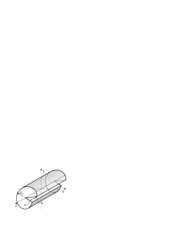
Figure 8: The combined wedge and screw dislocation. The picture is drawn for negative deficit angle $\theta$ and the Burgers vector $b$ which is antiparallel to the $Z$ axis.

Then the lower side of the cut is moved along the $Z$ axis in the opposite direction on the distance $b=2\pi c$, where $b$ is the Burgers vector, and both sides of the cut are glued together. The cut out or added wedge of media corresponds to the wedge dislocation, and the displacement of the lower side of the cut along the $Z$ axis describes the screw dislocation. Both types of dislocations are experimentally observed defects in real crystals (see i.e. [20]). Thus, metric (34) qualitatively describes nontrivial geometry around combined wedge and screw dislocations. For this metric, we can construct triad field and the corresponding torsion tensor which is equal to the surface density of the Burgers vector.

We used the word “qualitatively” because a solution of Einstein’s equations can be written in an arbitrary coordinate system and does not depend on Lame coefficients which characterize the elastic properties of media. The coordinate transformation (33) describes only cut and paste process of defect creation. In reality, the media comes to the equilibrium state after gluing both sides of the cut, and this process is driven by the elasticity theory equations. Therefore, the induced metric must depend on Lame coefficients. To consolidate gravity and elasticity theories we proposed to use the elastic gauge [8]. It is given by the following construction. First, we fix the cylindrical coordinates $\rho,\psi,\zeta$ in the Euclidean space related to the considered problem. The flat metric and the triad field are marked with a circle over a symbol

$$\begin{split}ds^{2}&=\overset{\circ}{g}{}_{\mu\nu}dx^{\mu}dx^{\nu}=d\rho^{2}+\rho^{2}d\psi^{2}+d\zeta^{2},\\ \overset{\circ}{e}{}_{\mu}{}^{i}&=\begin{pmatrix}1&0&0\\ 0&\rho&0\\ 0&0&1\end{pmatrix}\end{split}$$

Then the elastic gauge is chosen to be

$$\overset{\circ}{g}{}^{\mu\nu}\overset{\circ}{\nabla}_{\mu}e_{\nu i}+\frac{\sigma}{1-2\sigma}\overset{\circ}{e}{}^{\mu}{}_{i}\overset{\circ}{\nabla}_{\mu}e^{T}=0,$$ (35)

where a circle over the covariant derivative $\overset{\circ}{\nabla}{}_{\mu}$ means that it is constructed for flat metric $\overset{\circ}{g}{}_{\mu\nu}$; $e^{T}=\overset{\circ}{e}{}^{\mu}{}_{i}e_{\mu}{}^{i}$, and $\sigma={\sf\,const}$ is the Poisson ratio defined by the Lame coefficients [22].

Physical meaning of this gauge condition is based on the linear approximation. Suppose defects are absent, and we have only elastic deformations described by the displacement vector field $u^{i}(x)$ which parameterizes diffeomorphisms of ${\mathbb{R}}^{3}$. For simplicity, we assume that it is given in the Cartesian coordinate system. Than, for small relative displacements $|\partial_{\mu}u^{i}|\ll 1$, the induced triad field can be chosen in the form (there is a freedom in local ${\mathbb{S}}{\mathbb{O}}(3)$ rotations):

$$e_{\mu i}\approx\delta_{\mu i}-\frac{1}{2}(\partial_{\mu}u_{i}+\partial_{i}u_{\mu}).$$ (36)

In the linear approximation in Cartesian coordinates, Latin and Greek indices may be identified. Then the elastic gauge condition (35) reduces to the usual linear elasticity theory equations for the displacement vector field [22]

$$(1-2\sigma)\triangle u_{i}+\partial_{i}\partial_{j}u^{j}=0,$$ (37)

and the reduction of Eq. (35) to Eq. (37) is quite obvious. Introduction of flat covariant derivatives in the elastic gauge (35) allows us to use arbitrary coordinate systems.

The triad field corresponding to metric (34) is

$$e_{\mu}{}^{i}=\begin{pmatrix}\dfrac{\raise-3.01385pt\hbox{$1$}}{\raise 3.01385pt\hbox{$\alpha$}}&0&0\\ 0&f&-c\\ 0&0&1\end{pmatrix}.$$ (38)

The $f,\psi$ part of the triad corresponds to the symmetrized linear approximation (36), and the constant unsymmetrical $\psi$ part does not alter the form of the elastic gauge condition. We change the radial coordinate $f=f(\rho)$ to rewrite the triad in the elastic gauge. Then the elastic gauge condition (35) reduces to the Euler ordinary differential equation

$$\frac{f^{\prime\prime}}{\alpha}\left(1+\frac{\sigma}{1-2\sigma}\right)+\frac{f^{\prime}}{\rho}\left(\frac{1}{\alpha}+\frac{\sigma}{1-2\sigma}\right)-\frac{f}{\rho^{2}}\left(1+\frac{\sigma}{1-2\sigma}\right)=0.$$ (39)

This is the same equation which arises for pure wedge dislocation [8] (the interested reader can find more details there). To uniquely fix the solution of this equation, we suppose that the media fills only the cylinder of finite radius $R_{0}$ (this is needed to avoid divergences) and impose two additional gauge conditions

$$e_{\rho}{}^{\rho}|_{\rho=R_{0}}=1,~{}~{}~{}~{}e_{\psi}{}^{\psi}|_{\rho=0}=0.$$

The first gauge condition means the absence of external forces on the surface of the cylinder, and the second one corresponds to the absence of the angular component of the deformation tensor at the core of dislocation. Afterwards, the solution of Eq.(39) is uniquely defined

$$f=\frac{\alpha}{\gamma R_{0}^{\gamma-1}}\rho^{\gamma},$$

where

$$\gamma=-\theta B+\sqrt{\theta^{2}B^{2}+1+\theta},~{}~{}~{}~{}B=\frac{\sigma}{2(1-\sigma)}.$$

Thus, the Euclidean version of the BTZ solution for zero cosmological constant (34) in the elastic gauge (35) becomes

$$ds^{2}=\left(\frac{\rho}{R_{0}}\right)^{2(\gamma-1)}d\rho^{2}+\left(\frac{\alpha^{2}}{\gamma^{2}}\left(\frac{\rho}{R_{0}}\right)^{2(\gamma-1)}\rho^{2}+c^{2}\right)d\psi^{2}+d\zeta^{2}-2cd\zeta d\psi.$$ (40)

This is the exact solution of the Euclidean Einstein equations written in the elastic gauge. It describes the induced metric around combined wedge and screw dislocations and nontrivially depends on the Poisson ratio characterizing the elastic properties of media. Below, this solution is compared with the result obtained entirely within the elasticity theory without referring to Einstein equations.

The wedge and screw dislocations are relatively simple linear defects in solids, and the corresponding displacement vector field can be explicitly found as the solution to the linear elasticity field equations (37). The results are well known, and we skip their derivation. The displacement vector field for the wedge dislocation in cylindrical coordinates $R,\Phi,Z$ is [21]

$$u_{R}^{(\text{wedge})}=-\theta\frac{1-2\sigma}{2(1-\sigma)}\rho\ln\frac{\rho}{{\sf\,e}R_{0}},~{}~{}~{}~{}u_{\Psi}^{(\text{wedge})}=-\theta\rho\phi,~{}~{}~{}~{}u_{Z}^{(\text{wedge})}=0,$$ (41)

where ${\sf\,e}$ is the base of the natural logarithm. The displacement vector field for the screw dislocation is [22]

$$u_{R}^{(\text{screw})}=u_{\Phi}^{(\text{screw})}=0,~{}~{}~{}~{}u_{Z}^{(\text{screw})}=c\phi=\frac{b}{2\pi}\phi,$$ (42)

where $b$ is the Burgers vector. The displacements vectors can be added in the linear elasticity theory, and the total displacement vector for combined wedge and screw dislocations becomes

$$u=u^{(\text{wedge})}+u^{(\text{screw})}.$$

In our notations, the coordinate transformation corresponding to this displacement vector field is

$$R=\rho-u_{R},~{}~{}~{}~{}\Phi=\phi-\frac{1}{\rho}u_{\Phi},~{}~{}~{}~{}Z=\zeta-u_{Z}.$$

The induced metric within the elasticity theory becomes

$$\begin{split}ds^{2}_{\text{(elastic)}}&=dR^{2}+R^{2}d\Phi^{2}+dZ^{2}=\\ &=\left(1+\theta\frac{1-2\sigma}{1-\sigma}\ln\frac{\rho}{R_{0}}\right)d\rho^{2}+\left[\rho^{2}\left(1+\theta\frac{1-2\sigma}{1-\sigma}\ln\frac{\rho}{R_{0}}+\theta\frac{1}{1-\sigma}\right)+c^{2}\right]d\phi^{2}\\ &+d\zeta^{2}-2cd\zeta d\phi.\end{split}$$ (43)

The linear elasticity theory equations are valid for small relative displacements $\partial_{\mu}u^{i}\ll 1$. Therefore, the induced metric in the elasticity theory is expected to give correct answer for small deficit angle $\theta\ll 1$, small Burgers vector $b/R_{0}\ll 1$, and near the surface of the cylinder $\rho\sim R_{0}$.

To compare metrics (40) and (43), it is enough to consider small deficit angles. For $\theta\ll 1$,

$$\gamma\approx 1+\theta\frac{1-2\sigma}{2(1-\sigma)}.$$

Expanding expression (40) in $\theta$, we obtain metric (43) in the linear approximation.

So, the elasticity theory induced metric reproduces only the linear approximation of the exact solution of the Euclidean Einstein’s equations within the geometric theory of defects. Metric (40) obtained within the geometric approach is simpler in its form, valid for the whole range of radius $0<\rho<R_{0}$, all deficit angles $-1<\theta<\infty$, and Burgers vectors $b$. The components of the induced metric are proportional to the stress tensor of media. Therefore, the result obtained within the geometric theory of defects can be verified experimentally.

6 Conclusion

We considered the BTZ black hole solution for zero cosmological constant in detail. This case describes the interior region of the BTZ black hole and is simple enough to perform all calculation explicitly. We showed that points at $r=0$ are just coordinate singularities, and all geometric quantities are regular there, while the line $r=r_{-}$ corresponding to the inner horizon is singular: these points are not points of a manifold. There are four cones at each point of the line $r=r_{-}$. The singularity arises only after the identification of the polar angle $\varphi\sim\varphi+2\pi$.

The singularity structure is probably the same in a general case for negative cosmological constant, though it is analyzed only for zero cosmological constant.

In the Euclidean case, the BTZ solution for zero cosmological constant breaks into two disjoint manifolds along the horizon $r=r_{-}$ with Euclidean and Lorentzian signature metrics. The manifold with the Euclidean signature metric has straightforward physical interpretation in the geometric theory of defects describing combined wedge and screw dislocations in crystals. We showed that the induced metric obtained entirely within the ordinary elasticity theory provides only the linear approximation for the exact solution of Einstein’s equations. The Euclidean metric in the elastic gauge obtained from the BTZ solution depends nontrivially on Lame coefficients and can be measured experimentally.

The Euclidean version of the BTZ solution for negative cosmological constant has also straightforward interpretation in the geometric theory of defects, but in this case it describes continuous distribution of dislocations and is not so visual.

Acknowledgments. We are grateful to I. L. Shapiro for discussions. One of the authors (M.K.) thanks the Universidade Federal de Juiz de Fora for the hospitality, the FAPEMIG, the Russian Foundation of Basic Research (Grant No. 05-01-00884), and the Program for Supporting Leading Scientific Schools (Grant No. NSh-6705.2006.1) for financial support.

References

- [1] M. Bañados, C. Teitelboim, and J. Zanelli. Black hole in three-dimensional spacetime. Phys. Rev. Lett., 69(13):1849–1851, 1992.
- [2] E. Ayon-Beato, C. Martinez, and J. Zanelli. Phys. Rev. D70, 044027, 2004.
- [3] S. Carlip. Quantum Gravity in Dimensions. Cambridge University Press, Cambridge, 1998.
- [4] M. Bañados, M. Henneaux, C. Teitelboim, and J. Zanelli. Geometry of the black hole. Phys. Rev., D48(4):1506–1525, 1993.
- [5] A. R. Steif. Supergeometry of three-dimensional black holes. Phys. Rev. D, 53(10):5521–5526, 1996.
- [6] M. O. Katanaev and I. V. Volovich. Theory of defects in solids and three-dimensional gravity. Ann. Phys., 216(1):1–28, 1992.
- [7] M. O. Katanaev and I. V. Volovich. Scattering on dislocations and cosmic strings in the geometric theory of defects. Ann. Phys., 271:203–232, 1999.
- [8] M. O. Katanaev. Wedge dislocation in the geometric theory of defects. Theor. Math. Phys., 135(2):733–744, 2003.
- [9] M. O. Katanaev. One-dimensional topologically nontrivial solutions in the Skyrme model. Theor. Math. Phys., 138(2):163–176, 2004.
- [10] M. O. Katanaev. Geometric theory of defects. Physics – Uspekhi, 48(7):675–701, 2005.
- [11] J. A. Wolf. Spaces of constant curvature. University of California, Berkley, California, 1972.
- [12] A. Staruszkiewicz. Gravitational theory in three-dimensional space. Acta Phys. Polon., 24(6(12)):735–740, 1963.
- [13] G. Clemént. Field–theoretic particles in two space dimensions. Nucl. Phys., B114:437–448, 1976.
- [14] S. Deser, R. Jackiw, and G. ’t Hooft. Three-dimensional Einstein gravity: Dynamics of flat space. Ann. Phys., 152(1):220–235, 1984.
- [15] M. O. Katanaev. Global solutions in gravity. Lorentzian signature. Proc. Steklov Inst. Math., 228:158–183, 2000.
- [16] C. Farina, J. Gamboa, and A. J. Seguí-Santonja. Motion and trajectories of particles around three-dimensional black holes. Class. Quantum Grav., 10(11):L193–L200, 1993.
- [17] N. Cruz, C. Martínez, and L. Peña. Geodesic structure of the black hole. Class. Quantum Grav., 11(11):2731–2740, 1994.
- [18] S. Carlip and C. Teitelboim. Aspects of black hole quantum mechanics and thermodynamics in 2+1 dimensions. Phys. Rev. D, 51(2):622–631, 1995.
- [19] M. O. Katanaev, T. Klösch, and W. Kummer. Global properties of warped solutions in general relativity. Ann. Phys., 276:191–222, 1999.
- [20] S. Amelinckx. The direct observation of dislocations. Academic Press, New York and London, 1964.
- [21] A. M. Kosevich. Physical mechanics of real crystals. Naukova dumka, Kiev, 1981. [in Russian].
- [22] L. D. Landau and E. M. Lifshits. Theory of Elasticity. Pergamon, Oxford, 1970.