RADIATION AND POTENTIAL BARRIERS OF A 5D BLACK STRING SOLUTION

Abstract

By using a massless scalar field we examine the effect of an extra dimension on black hole radiation. Because the equations are coupled, we find that the structure of the fifth dimension (as for membrane and induced-matter theory) affects the nature of the radiation observed in four-dimensional spacetime. In the case of the Schwarzschild-de Sitter solution embedded in a Randall-Sundrum brane model, the extension of the black hole along the fifth dimension looks like a black string. Then it is shown that, on the brane, the potential barrier surrounding the black hole has a quantized as well as a continuous spectrum. In principle, Hawking radiation may thus provide a probe for higher dimensions.

PACS Nos.: 04.70.Dy, 04.50.+h

1 Introduction

Hawking radiation is one of the most important predictions in black hole physics. A simple proof of it was given by Damour and Ruffini [1] who used a tortoise coordinate to write the radial part of the Klein-Gordon equation in the form of the $Schr\ddot{o}dinger-like$ equation, and then found that there is a potential barrier outside the horizon, and hence implies that black holes can radiate. There is a long list of research papers on this in the literature [2] [3] [4]. In the presence of a cosmological constant $\Lambda$, the Schwarzschild solution is replaced by the Schwarzschild-de Sitter solution which contains two event horizons — an inner black hole horizon and an outer cosmological horizon. We are living in between these two horizons. It is known that Hawking radiation also exists in this case [5] [6] [7]. However, because $\Lambda$ is small, its influence on the radiation is expected to be small, too.

In Kaluza-Klein as well as string/brane theories, it is assumed that there exists compact or non-compact extra spatial dimensions. It is known that the 4D Schwarzschild-de Sitter black hole solution can be embedded into a 5D Ricci-flat manifold with the following metric [8] [9] [10]

$$dS^{2}=\frac{\Lambda\xi^{2}}{3}\left[f(r)dt^{2}-\frac{1}{f(r)}dr^{2}-r^{2}\left(d\theta^{2}+\sin^{2}\theta d\phi^{2}\right)\right]-d\xi^{2},$$ (1)

where

$$f(r)=1-\frac{2M}{r}-\frac{\Lambda}{3}r^{2}.$$ (2)

The term inside the square bracket is exactly the same line-element as the 4D Schwarzschild-de Sitter solution. Therefore, when viewed from a $\xi=constant$ hypersurface, the 4D line-element represents exactly the Schwarzschild-de Sitter black hole. However, when viewed from 5D, the horizon does not form a 4D sphere. It looks like a black string lying along the fifth dimension. Usually, people call the solution of the 5D equation $R_{AB}=\Lambda g_{AB}$ the 5D Schwarzschild-de Sitter solution. Therefore, to distinguish it, we call the solution (1) a black string, or more precisely, a 5D Ricci-flat Schwarzschild-de Sitter solution, because (1) satisfies the 5D vacuum equation $R_{AB}=0$. So, for (1) there is no cosmological constant when viewed from 5D. However, when viewed from 4D, there is an effective cosmological constant. This solution has been studied in many works [11] [12] [13] [14] focusing mainly on the induced cosmological constant, the extra force and so on. To our knowledge, no one has studied the radiation of this 5D solution before. Because the black hole radiation could hopefully be detected in the near future, and because recent cosmological observations favor the $\Lambda$ model for dark energy, here we will study the black hole radiation of this 5D solution.

This paper is organized as follows. In Section 2, we use the method of separation of variables to analyze the 5D Klein-Gordon equation. In section 3, we use the R-S type brane model as a boundary condition to solve the equation for the fifth dimension. In section 4, we return to the radial equation and obtain the potential barrier and analyze its spectrum. Section 5 is a discussion.

2 The Klein-Gordon Equation in the 5D Schwarzschild-de Sitter Solution

We use a coordinate transformation

$$\xi=\sqrt{\frac{3}{\Lambda}}e^{\sqrt{\frac{\Lambda}{3}}y}$$ (3)

and rewrite the 5D metric (1) as

$$dS^{2}=e^{2\sqrt{\frac{\Lambda}{3}}y}\left[f(r)dt^{2}-\frac{1}{f(r)}dr^{2}-r^{2}\left(d\theta^{2}+\sin^{2}\theta d\phi^{2}\right)-dy^{2}\right],$$ (4)

where y is the new coordinate of the fifth dimension. The horizons of the 5D metric (4) are on the hypersurface $f(r)=0$, which has three solutions

$$f(r)=\frac{\Lambda}{3r}(r-r_{e})(r_{c}-r)(r-r_{o}).$$ (5)

Here $r_{e}$ is the black hole horizon, $r_{c}$ is the cosmological horizon, and we are living in between these two horizons. Another solution $r_{o}=-(r_{e}+r_{c})$ is negative and physically meaningless.

We consider a massless scalar field $\Phi$ in the 5D spacetime (4). The Klein-Gordon equation for $\Phi$ is

$$\square\Phi=0,$$ (6)

where $\square=\frac{1}{\sqrt{g}}\frac{\partial}{\partial x^{A}}\left(\sqrt{g}g^{AB}\frac{\partial}{\partial{x^{B}}}\right)$ is the 5D d’Alembertian operator. Using the method of separation of variables, we make the ansatz [15]

$$\Phi=\frac{1}{\sqrt{4\pi\omega}}\frac{1}{r}R_{\omega}(r,t)L(y)Y_{lm}(\theta,\phi).$$ (7)

Then Eq. (6) reduces to three equations:

$$\frac{d^{2}L(y)}{dy^{2}}+\sqrt{3\Lambda}\frac{dL(y)}{dy}+\Omega L(y)=0,$$ (8)

$$-\frac{1}{f(r)}r^{2}\frac{\partial^{2}}{\partial t^{2}}\left(\frac{R_{\omega}}{r}\right)+\frac{\partial}{\partial r}\left(r^{2}f(r)\frac{\partial}{\partial{r}}\left(\frac{R_{\omega}}{r}\right)\right)-\left[\Omega r^{2}+l(l+1)\right]\frac{R_{\omega}}{r}=0,$$ (9)

$$\frac{1}{\sin\theta}\frac{\partial}{\partial\theta}\left(\sin\theta\frac{\partial{Y_{lm}}}{\partial\theta}\right)+\frac{1}{\sin^{2}\theta}\frac{\partial^{2}Y_{lm}}{\partial{\phi^{2}}}=-l(l+1)Y_{lm},$$ (10)

where $\Omega$ and $\l$ are the two separation constants to be determined later, after the application of a boundary condition.

3 The Wave Function $L(y)$

The wave function $L(y)$ is governed by Eq. (8) which is a linear second-order differential equation with constant coefficients and can be rewritten as

$$\frac{d^{2}}{dy^{2}}[e^{\frac{\sqrt{3\Lambda}}{2}y}L(y)]+(\Omega-\frac{3\Lambda}{4})[e^{\frac{\sqrt{3\Lambda}}{2}y}L(y)]=0.\\$$ (11)

Then, for the three cases $\Omega>\frac{3\Lambda}{4}$, $\Omega=\frac{3\Lambda}{4}$, and $\Omega<\frac{3\Lambda}{4}$, we obtain

$$L(y)=\left\{\begin{array}[]{c}Ce^{-\frac{\sqrt{3\Lambda}}{2}y}\cos\left[\sqrt{\Omega-\frac{3}{4}\Lambda}(y-y_{0})\right],{\ \ \ \ \ }{\ \ \ }\text{\ for }\Omega>\frac{3\Lambda}{4},\\ \left(C_{1}+C_{2}y\right)e^{-\frac{\sqrt{3\Lambda}}{2}y},{\ \ \ \ \ \ \ \ \ \ \ \ \ \ }{\ \ \ \ \ \ \ \ \ \ \ \ \ }\text{\ for }\Omega=\frac{3\Lambda}{4},\\ C_{3}e^{\frac{-\sqrt{3\Lambda}+\sqrt{3\Lambda-4\Omega}}{2}y}+C_{4}e^{\frac{-\sqrt{3\Lambda}-\sqrt{3\Lambda-4\Omega}}{2}y},\text{\ \ \ \ for }\Omega<\frac{3\Lambda}{4},\\ \end{array}\right.$$ (12)

where $(C,y_{0})$, $(C_{1},C_{2})$ and $(C_{3},C_{4})$ are the three pairs of integration constants for the three equations in Eqs. (12), respectively.

Because $L(y)$ represents the wave function along the $y$-direction for a massless scalar particle and $|L(y)|^{2}$ represents the probability of finding the particle, a boundary condition should be used to make $L(y)$ finite everywhere. A simple way is to use the R-S two-brane model [16] [17], in which the fifth dimension is a line segment. The length of this line could be very small [16], or could be very large [17]. We suppose that the two branes are at $y=0$ and $y=y_{1}$, respectively, and that we live on the $y=0$ brane. Then $L(y)$ should reach its maximum at $y=0$. It is shown that the first equation in Eqs. (12) gives a discrete spectrum for $L(y)$, and the second and third equations give continuous spectra. We discuss them in the following subsections.

3.1 Discrete Spectra $(\Omega>\frac{3\Lambda}{4})$

For the first solution of Eqs. (12), it is expected that the wave function $L(y)$ should reach its maximum on our brane $y=0$, and hence $y_{0}=0$ is obtained. Then we expect that the cosine function in Eqs. (12) looks like a standing wave between the two branes, so we have

$$y_{1}\sqrt{\Omega-\frac{3}{4}\Lambda}=n\pi,{\ \ \ }n=1,2,3\cdots,\\$$ (13)

and the quantized discrete spectra for $\Omega$ and $L(y)$ are obtained as follows:

$$\Omega_{n} = \frac{n^{2}\pi^{2}}{y_{1}^{2}}+\frac{3}{4}\Lambda,{\ \ \ }n=1,2,3\cdots,$$ (14)

$$L_{n}(\phi) = Ce^{-\frac{\sqrt{3\Lambda}}{2}y}\cos\left(n\pi\frac{y}{y_{1}}\right),{\ \ \ }n=1,2,3\cdots,$$ (15)

It is easy to verify that the corresponding eigenvalue equation and the operator for $\Omega_{n}$ are

$$\hat{\Omega}L_{n}(y)=\Omega_{n}L_{n}(y),{\ \ \ }\hat{\Omega}=-\frac{d}{dy}\left(\frac{d}{dy}+\sqrt{3\Lambda}\right).$$ (16)

For $n=1$, the first (ground) eigenfunction is $L_{1}(y)=Ce^{-\frac{\sqrt{3\Lambda}}{2}y}\cos(\frac{\pi{y}}{y_{1}})$. For $n=2$ and $n=3$, the second and third eigenfunctions are $L_{2}=Ce^{-\frac{\sqrt{3\Lambda}}{2}y}\cos(\frac{2\pi{y}}{y_{1}})$ and $L_{3}(y)=Ce^{-\frac{\sqrt{3\Lambda}}{2}y}\cos(\frac{3\pi{y}}{y_{1}})$, respectively. These three eigenfunctions are plotted in Fig. 1. It is clear that $L_{n}(y)$ starts from the value $L_{n}(y)=1$ but does not end exactly at the value $L_{n}(y)=\pm 1$. This is due to the effect of the exponential factor $e^{-\frac{\sqrt{3\Lambda}}{2}y}$ in $L_{n}(y)$ in Eq. (15).

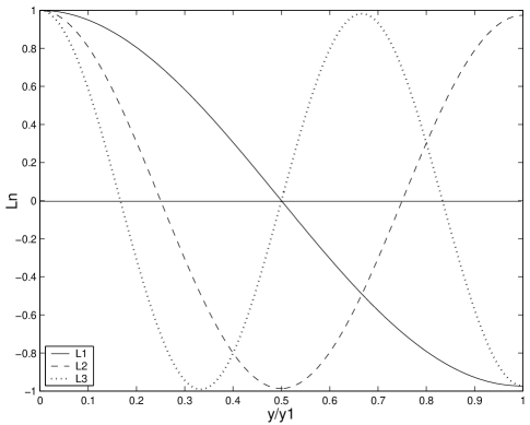
Figure 1: The first three eigenfunctions of $L_{n}(y)$: $L_{1}$(solid), $L_{2}$(dashed), and $L_{3}$(dotted) with $C=1$ and $\Lambda=10^{-3}$. For illustration, a very large 5th dimension with $y_{1}=1$ is used here.

3.2 Continuous Spectra $(\Omega\leq\frac{3\Lambda}{4})$

For $\Omega\leq\frac{3}{4}\Lambda$, the wave function $L(y)$ is given by the last two equations in Eqs. (12). We rewrite these as follow:

$$L(y)=\left\{\begin{array}[]{c}\left(C_{1}+C_{2}y\right)e^{-\frac{\sqrt{3\Lambda}}{2}y},\text{ \ \ }\text{ \ \ }\text{ \ \ \ }\text{ \ \ \ \ \ \ }\text{ \ \ \ \ \ }\text{ \ for }{\ \ }\Omega=\frac{3}{4}\Lambda,\\ C_{3}e^{\frac{-\sqrt{3\Lambda}+\sqrt{3\Lambda-4\Omega}}{2}y}+C_{4}e^{\frac{-\sqrt{3\Lambda}-\sqrt{3\Lambda-4\Omega}}{2}y},\text{ \ for }{\ \ }\Omega<\frac{3}{4}\Lambda.\\ \end{array}\right.$$ (17)

Because $\Omega$ is continuous, the wave function $L(y)$ is also continuous. Here, just as the discrete case, we require that the wave function $L(y)$ starts from the maximum on the $y=0$ brane and decreases as $y$ increases. Under this requirement the case $\Omega=\frac{3}{4}\Lambda$ contains two modes: for ($C_{1}=1,C_{2}=0$), $L(y)$ decreases slightly because of the small $\Lambda$. For ($C_{1}=0,C_{2}<0$), it decreases almost linearly to $y$. The $\Omega<\frac{3}{4}\Lambda$ case is a little more complicated because both $y$ and $\Omega$ can vary. The significant variation can be illustrated in Fig. 2 where $C_{1}=-1$, $C_{2}=2$ and $y_{1}=1$ are chosen.

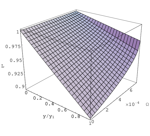
Figure 2: The continuous wave function L(y,$\Omega$) for $\Omega<\frac{3}{4}\Lambda$ with $C_{3}=-1$, $C_{4}=2$, $\Lambda=10^{-3}$ and $y_{1}=1$ (a very large 5th dimension).

4 The Radial Equation and Quantized Potential

Now we return to the radial Eq. (9). Here $t$ can be eliminated by using

$$R_{\omega}(r,t)\rightarrow\Psi_{\omega l}(r)e^{-i\omega t},$$ (18)

and hence Eq. (9) is rewritten as

$$\left[-f(r)\frac{d}{dr}(f(r)\frac{d}{dr})+V(r)\right]\Psi_{\omega l}(r)=\omega^{2}\Psi_{\omega l}(r),$$ (19)

where the potential is given by

$$V(r)=f(r)\left[\frac{1}{r}\frac{df(r)}{dr}+\frac{l(l+1)}{r^{2}}+\Omega\right].$$ (20)

Furthermore, we introduce the tortoise coordinate

$$x=\frac{1}{2M}\int\frac{dr}{f(r)}.$$ (21)

Integrating this equation shows that $x$ can be expressed explicitly in the following form:

$$x=\frac{1}{2M}\left[\frac{1}{2K_{e}}\ln\left(\frac{r}{r_{e}}-1\right)-\frac{1}{2K_{c}}\ln\left(1-\frac{r}{r_{c}}\right)+\frac{1}{2k_{o}}\ln\left(1-\frac{r}{r_{o}}\right)\right],$$ (22)

where

$$K_{i}=\frac{1}{2}\left|\frac{df}{dr}\right|_{r=r_{i}},$$ (23)

explicitly as

$$K_{e}=\frac{(r_{c}-r_{e})(r_{e}-r_{o})}{6r_{e}}\Lambda,$$ (24)

$$K_{c}=\frac{(r_{c}-r_{e})(r_{c}-r_{o})}{6r_{c}}\Lambda,$$ (25)

$$K_{o}=\frac{(r_{o}-r_{e})(r_{c}-r_{o})}{6r_{o}}\Lambda.$$ (26)

Under the tortoise coordinate transformation (21), the radial Eq. (19) reads

$$\left[-\frac{d^{2}}{dx^{2}}+4M^{2}V(r)\right]\Psi_{\omega l}(x)=4M^{2}\omega^{2}\Psi_{\omega l}(x).$$ (27)

This is a $Schr\ddot{o}dinger-like$ equation which describes a one-dimensional wave propagating between the black hole horizon $r_{e}$ and the cosmological horizon $r_{c}$. The potential barrier $V(r)$ determines the reflection and the transmission coefficients of the scalar massless particles, and the non-zero reflection coefficient indicates the existence of Hawking radiation.

Now we consider the potential barrier $V(r)$ (20) where $\Omega$ can take a continues value if $\Omega\leq\frac{3}{4}\Lambda$, or a discrete value if $\Omega>\frac{3}{4}\Lambda$. In the latter discrete case, $V(r)$ takes the form

$$V_{n}(r)=f(r)\left[\frac{1}{r}\frac{df(r)}{dr}+\frac{l(l+1)}{r^{2}}+\frac{n^{2}\pi^{2}}{y_{1}^{2}}+\frac{3}{4}\Lambda\right].$$ (28)

From this equation it is obvious that if $y_{1}$ is very small, the potential barrier $V_{n}$ will be very large. However, the potential barrier for the 4D Schwarzschild-de Sitter solution corresponds to $\Omega=0$. To make the 5D and 4D cases comparable, a very large 5th dimension for $y_{1}$ have to be chosen. This enables us to plot the first three quantized potential barriers $V_{n}(r)$, as well as the 4D ($\Omega=0$) case, in Fig. 3.

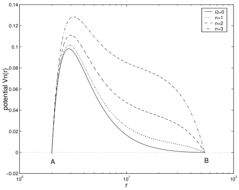
Figure 3: The first three potential barriers $V_{n}(r)$ with $n=1$ (dotted), $n=2$ (dashed), and $n=3$ (dash-dot) with $l=1$, $M=1$, $\Lambda=10^{-3}$ and $y_{1}=10^{3/2}$ (a very large 5th dimension). The potential barriers of the corresponding 4D solution ($\Omega=0$) is also plotted for comparison. The black hole horizon (point A) has $r_{e}\sim 2$ and the cosmological horizon (point B) has $r_{c}\sim 54$ and the potential tends to zero quickly as $x\rightarrow\pm\infty.$

5 Discussion

The 4D Schwarzschild-de Sitter black hole solution can be embedded into the 5D Ricci-flat solution (1). We have analyzed the nature of a massless scalar particle moving in the 5D solution (1), by solving the corresponding 5D Klein-Gordon Eq. (6) under the assumption of separability. We have assigned boundary condition in the 5th dimension by using a two-brane Randall-Sundrum model. The separation constant $\Omega$ in Eq. (8) for the extra dimension plays a critical role, since its value leads to both quantized and continuous spectra. When $\Omega$ is inserted into the radial Eq. (9), we find that by using the tortoise coordinate (21) we obtain a one-dimensional $Schr\ddot{o}dinger-like$ Eq. (27) in which quantized potential barriers differ significantly from the usual 4D case. (The latter is recovered for $\Omega=0$, whereas in the 5D case $\Omega$ takes discrete values for $\Omega>3\Lambda/4$ and continuous values for $\Omega\leq 3\Lambda/4$.) Now in a usual language, as the potential barrier becomes higher, the reflection of waves become more efficient and the black hole radiation is more intensive. Thus we conclude that the existence and structure of the 5th dimension can in principle be investigated by data about the 4D Hawking radiation around black hole.

Here we should emphasize that in the brane-world scenario, all standard particles and forces, except gravity, are confined on the branes. This implies that the 5D energy and pressure densities (including a possible positive or negative cosmological constant) are singular at the branes. Usually, this is treated by using their 4D counterparts (which are finite) multiplied by a delta function. It is known that a delta function can be approximately described by a series of periodic function. In this case, although the delta function itself is singular at the brane, each of its component function is not necessarily be singular there. In other words, if we only focus on a single mode of the series, the wave function for this mode may reach the maximum value but keep smooth and finite at the brane. With this purpose in mind, we have used the RS2-type brane model to give the required boundary conditions. This is because in the RS2 brane model, the 5th dimension $y$ could be very large and the second brane could be pushed far away even to infinity. This is just what we want in our paper because the potential barrier $V_{n}(r)$ tends to its 4D GR value for $y_{1}\rightarrow\infty$ as can be seen from Eq. (28). Meanwhile, the 4D spacetime on the brane in our case takes exactly the same form as the 4D Schwarzschild-de Sitter solution which is 5D empty. Therefore, there would be no brane if we do not consider the contribution of the wave function of the scalar field. The wave function, especially $L(y)$, plays the role to provide a kind of brane which is similar to the one in the RS2 model. For instance, a suitable superposition of some of the quantized or/and continuous components of $L(y)$ may provide a wave function which is very large at $y=0$ and drops rapidly for $y\neq 0$ and thus forms a practical brane at the $y=0$ hypersurface.

6 Acknowledgments

We are grateful to Feng Luo for valuable discussions. This work was supported by NSF(10573003) and NBRP(2003CB716300) of P. R. China and by NSERC of Canada. Xu was supported in part by DUT 893321.

7 References

References

- [1] T. Damour, R. Ruffini, Phys. Rev. D 14, 332 (1976).
- [2] Don N. Page, New J. Phys. 7, 203 (2005), (hep-th/0409024) and references therein.
- [3] A. Higuchi, G.E.A. Matsas, D. Sudarsky, Phys. Rev. D 58, 104021 (1998), gr-qc/9806093.
- [4] L.C.B. Crispino, A. Higuchi, G.E.A. Matsas, Class. Quant. Grav. 17, 19 (2000).
- [5] P.R. Brady, C.M. Chambers, W.G. Laarakkers, E. Poission, Phys. Rev. D 60, 064003 (1999), gr-qc/9902010.
- [6] I. Brevik, B. Simonsen, Gen. Rel. Grav. 33, 1839 (2001).
- [7] J.X. Tian, Y.X. Gui, G.H. Guo, Gen. Rel. Grav. 35, 1471 (2003).
- [8] B. Mashhoon, H.Y. Liu, P.S. Wesson, Phys. Lett. B. 331, 305 (1994).
- [9] H.Y. Liu, Gen. Rel. Grav. 23, 759 (1991).
- [10] P.S. Wesson, Space-Time-Matter (World Scientific, Singarpore, 1999).
- [11] B. Mashhoon, P.S. Wesson, H.Y. Liu, Gen. Rel. Grav. 30, 555 (1998).
- [12] P.S. Wesson, B. Mashhoon, H.Y. Liu, W.N. Sajko, Phys. Lett. B 456, 34 (1999).
- [13] H.Y. Liu, B. Mashhoon, Phys. Lett. A 272, 26 (2000), gr-qc/0005079.
- [14] B. Mashhoon, P.S. Wesson, Class. Quant. Grav. 21, 3611 (2004), gr-qc/0401002.
- [15] B.P. Jensen, P. Candelas, Phys. Rev. D 33, (1986) 1590.
- [16] L. Randall, R. Sundrum, Phys. Rev. Lett. 83, 3370 (1999), hep-ph/9905221.
- [17] L. Randall, R. Sundrum, Phys. Rev. Lett. 83, 4690 (1999), hep-th/9906064.