Thin Shell Wormhole in Heterotic String Theory

Abstract

Using ’ Cut and Paste ’ technique, we develop a thin shell wormhole in heterotic string theory. We determine the surface stresses, which are localized in the shell, by using Darmois-Israel formalism. The linearized stability of this thin wormhole is also analyzed.

Introduction:

Recently, several Physicists have given their attention to develop thin shell wormhole Models. Visser, the pioneer, presented this new class of wormholes by using ’Cut and Paste’ technique [1]. The model is constructed by surgically grafting two Schwarzschild spacetimes together in such a way that no event horizon is permitted to form . Taking two copies of region from Schwarzschild geometry with $r\geq a$ : $M^{\pm}\equiv(x|r\geq a)$ where $a>r_{h}$ [ $r_{h}$ = radius of event horizon and $\pm$ indicates two copies ], one can paste two copies $M^{\pm}$ together at the hypersurface $\Sigma=\Sigma^{\pm}=(x|r=a)$ results in a geodesically complete regions to make a thin shell wormhole. This construction creates a geodesically complete manifold $M=M^{+}\bigcup M^{-}$ with two asymptotically flat regions connected by a throat placed at $\Sigma$. In this case, the surface energy density of the shell is found to be negative (one can use Israel-Darmois [2] formalism to prove it). This indicates the presence of exotic matter in the throat. After some years of this proposal, Visser with his collaborator Poisson had analyzed the stability of thin shell wormhole constructed by joining the two Schwarzschild geometries [3]. Ishak and Lake have examined the stability of transparent spherical symmetric thin-shell wormholes [4] .

Eiroa and Romero [5] have studied the linear stability of charged thin shell wormholes constructed by joining the two Reissner-Nordström spacetimes under spherically symmetric perturbations. Lobo and Crawford [6] have extended the linear stability analysis to the thin shell wormholes with Cosmological Constant.
Eiroa and Simeone [7] have studied cylindrically symmetric thin shell wormhole geometries associated to gauge cosmic strings. Also, the same authors have constructed a charged thin shell wormhole in dilaton gravity and they have shown that the reduction of the total amount of exotic matter is dependent on the Dilaton-Maxwell coupling parameter [8]. The five dimensional thin shell wormholes in Einstein-Maxwell theory with a Gauss Bonnet term has been studied by Thibeault et al [9]. They have made a linearized stability analysis under radial perturbations. Recently, the present authors have studied thin shell wormholes in higher dimensional Einstein-Maxwell theory which is constructed by Cutting and Pasting two metrics corresponding to a higher dimensional Reissner-Nordström black hole [10].
Super string theory plays an important role to unify gravity with all other fundamental interactions in nature. In recent past, the general dyonic black hole solutions to the heterotic string theory were obtained by Jhatkar et al [11] and Cvetic et al [12]. They had given a general black hole solution to the Heterotic string compactified on a four dimensional torus. These black hole solutions exhibit several different properties compared to the Reissner-Nordström black holes. After the publication of the paper by Visser [1], there has been a growing interest in the study of thin shell wormholes constructed by black holes. And since, the charged black holes of general relativity and string theory are qualitatively different, it is expected that thin shell wormhole constructed by black holes in string theory will give new features. The purpose of this article is to study thin shell wormhole in heterotic string theory. We develop the model by cutting and pasting two metrics corresponding to a four dimensional dyonic black hole solution of toroidally compactified heterotic string theory. The linearized stability is analyzed under radial perturbations around static solutions.
The paper is organized as follows: The black hole solution in heterotic string theory is rewritten in section 2. In section 3, thin shell wormhole has been constructed by means of the Cut and Paste tactics. A linearized stability analysis is studied in section 4. In section 5, the total amount of exotic matter has been calculated. Section 6 is devoted to a brief summary and discussion.

2.Dyonic black holes in heterotic string theory

Following [11-13], we consider the metric which can be associated to a four dimensional Dyonic black hole solution of toroidally compactified heterotic string theory as

$$ds^{2}=-f(r)dt^{2}+\frac{dr^{2}}{f(r)}+h(r)d\Omega_{2}^{2}$$ (1)

where

$$f(r)=\frac{(r+b)(r-b)}{h(r)}$$ (2)

$$h^{2}(r)=(r+\hat{Q_{1}})(r+\hat{Q_{2}})(r+\hat{P_{1}})(r+\hat{P_{2}})$$ (3)

$$\hat{Q_{1}}=\sqrt{Q_{1}^{2}+b^{2}}$$ (4)

etc..

The above black hole consists with two independent electric charges $Q_{1}$ and $Q_{2}$ ( same signs ) as well as two independent magnetic charges $P_{1}$ and $P_{2}$. The position of the horizon is specified by the real positive parameter ’b’.
For the sake of simplicity, we do not include the 28 gauge fields to which the 28 components of charges are coupled.
The dilaton field takes the form [13]

$$e^{2\phi}=\frac{(r+\hat{P_{1}})(r+\hat{P_{2}})}{(r+\hat{Q_{1}})(r+\hat{Q_{2}})}$$ (5)

The above expression indicates that the dilaton field does not in general vanish for these solutions. It tends to zero asymptotically as $r\rightarrow\infty$ .

When $Q_{i}=P_{i}=0$, then the metric (1) reduces to Schwarzschild geometry:

$ds^{2}=-(1-\frac{2b}{R})dt^{2}+(1-\frac{2b}{R})^{-1}dR^{2}+R^{2}d\Omega_{2}^{2}$

While for $Q=Q_{i}=P_{i}\neq 0$, one can obtain

$ds^{2}=-(1-\frac{2\sqrt{Q^{2}+b^{2}}}{R}+\frac{b^{2}}{R^{2}})dt^{2}+(1-\frac{2\sqrt{Q^{2}+b^{2}}}{R}+\frac{b^{2}}{R^{2}})^{-1}dR^{2}+R^{2}d\Omega_{2}^{2}$,

which corresponds to Reissner-Nordström black hole geometry.

3. The Darmois-Israel formalism and Cut and Paste construction:

As we are interested to construct thin shell wormhole in heterotic string theory by using Cut and Paste technique, from the geometry (1), we take two copies of the region with $r\geq a$: $M^{\pm}=(x\mid r\geq a)$ where $a\geq r_{h}=b$ ( position of event horizon ) and paste the two pieces together at the hypersurface $\Sigma=\Sigma^{\pm}=(x\mid r=a)$.

This new construction results in a geodesically complete manifold $M=M^{+}\bigcup M^{-}$ with a matter shell at the surface $r=a$ , where the throat of the wormhole is located. Thus a single manifold M is obtained which connects two asymptotically flat regions at their boundaries $\Sigma$ and the throat is placed at $\Sigma$(here $\Sigma$ is a synchronous time like hypersurface). Following Darmois-Israel formalism, we shall determine the surface stresses at the junction boundary. The intrinsic coordinates in $\Sigma$ are taken as $\xi^{i}=(\tau,{\theta},\phi)$ with $\tau$ is the proper time on the shell. To understand the dynamics of the wormhole, we assume the radius of the throat be a function of the proper time $a=a(\tau)$. The parametric equation for $\Sigma$ is defined by

$$\Sigma:F(r,\tau)=r-a(\tau)$$ (6)

The second fundamental form ( extrinsic curvature ) associated with the two sides of the shell are

$$K_{ij}^{\pm}=-n_{\nu}^{\pm}\ [\frac{\partial^{2}X_{\nu}}{\partial\xi^{i}\partial\xi^{j}}+\Gamma_{\alpha\beta}^{\nu}\frac{\partial X^{\alpha}}{\partial\xi^{i}}\frac{\partial X^{\beta}}{\partial\xi^{j}}]|_{\Sigma}$$ (7)

where $n_{\nu}^{\pm}\$ are the unit normals to $\Sigma$ in M:

$$n_{\nu}^{\pm}=\pm|g^{\alpha\beta}\frac{\partial F}{\partial X^{\alpha}}\frac{\partial F}{\partial X^{\beta}}|^{-\frac{1}{2}}\frac{\partial F}{\partial X^{\nu}}$$ (8)

[ $i,j=1,2,3$ corresponding to boundary $\Sigma$ ; $\alpha,\beta=1,2,3,4$ corresponding to original spacetime ] with $n^{\mu}n_{\mu}=1$.

The intrinsic metric at $\Sigma$ is given by

$$ds^{2}=-d\tau^{2}+a(\tau)^{2}d\Omega^{2}$$ (9)

The position of the throat of the wormhole is described by $X^{\mu}=(t,a(t),\theta,\phi)$. The unit normal to $\Sigma$ is given by

$$n^{\nu}=(\frac{\dot{a}}{f(a)},\sqrt{(f(a)+\dot{a}^{2})},0,0)$$ (10)

Now using equations (1), (7) and (10), the non trivial components of the extrinsic curvature are given by

$$K_{\tau\tau}^{\pm}=\mp\frac{\frac{1}{2}f^{\prime}(a)+\ddot{a}}{\sqrt{(f(a)+\dot{a}^{2})}}$$ (11)

$$K_{\theta\theta}^{\pm}=K_{\phi\phi}^{\pm}=\pm\frac{h^{\prime}(a)}{2h(a)}\sqrt{(f(a)+\dot{a}^{2})}$$ (12)

We define jump of the discontinuity of the extrinsic curvature of the two sides of $\Sigma$ as $[K_{ij}]=K_{ij}^{+}-K_{ij}^{-}$ and $K=[K_{i}^{i}]=trace[K_{ij}]$.

The Ricci tensor at the throat can be calculated in terms of the discontinuity of the second fundamental forms ( extrinsic curvature ). This jump discontinuity, together with Einstein field equations, provides the stress energy tensor of $\Sigma$, where throat is localized: $T^{\mu\nu}=S^{\mu\nu}\delta(\eta)$ [ $\eta$ denotes the proper distance away from the throat ( in the normal direction )] with,

$$S_{j}^{i}=-\frac{1}{8\pi}([K_{j}^{i}]-\delta_{j}^{i}K)$$ (13)

where $S_{j}^{i}=diag(-\sigma,p_{\theta},p_{\phi})$ is the surface energy tensor with $\sigma$ , the surface density and $p_{\theta}$ and $p_{\phi}$, the surface pressures.

Now taking into account the equation (13), one can find

$$\sigma=-\frac{1}{4\pi}\frac{h^{\prime}(a)}{h(a)}\sqrt{f(a)+\dot{a}^{2}}$$ (14)

$$p_{\theta}=p_{\phi}=p=\frac{1}{8\pi}\frac{h^{\prime}(a)}{h(a)}\sqrt{f(a)+\dot{a}^{2}}+\frac{1}{8\pi}\frac{2\ddot{a}+f^{\prime}(a)}{\sqrt{f(a)+\dot{a}^{2}}}$$ (15)

[ over dot and prime mean, respectively, the derivatives with respect to $\tau$ and a ]

From equations (14) and (15), one can verify the energy conservation equation:

$$\frac{d}{d\tau}(\sigma h(a))+p\frac{d}{d\tau}(h(a))=0$$ (16)

or

$$\dot{\sigma}+\frac{\dot{h}(a)}{h(a)}(p+\sigma)=0$$ (17)

The first term represents the variation of the internal energy of the throat and the second term is the work done by the throat’s internal forces. Negative energy density in (14) implies the existence of exotic matter at the shell.

4. Linearized Stability Analysis:

Rearranging equation (14), we obtain the thin shell’s equation of motion

$$\dot{a}^{2}+V(a)=0$$ (18)

Here the potential is defined as

$$V(a)=f(a)-[\frac{4\pi h(a)\sigma(a)}{h^{\prime}(a)}]^{2}$$ (19)

4.1 Static Solution:

The above single dynamical equation (18) completely determines the motion of the wormhole throat. One can consider a linear perturbation around a static solution with radius $a_{0}$. We are trying to find a condition, for which stress energy tensor components at $a_{0}$ will obey null energy condition. For a static configuration of radius $a_{0}$, we obtain respective values of the surface energy density and the surface pressure by using the explicit form (1) of the metric as

$$\sigma_{0}=-\frac{1}{8\pi}\frac{\sqrt{(a_{0}+b)(a_{0}-b)}}{[(a_{0}+\hat{Q_{1}})(a_{0}+\hat{Q_{2}})(a_{0}+\hat{P_{1}})(a_{0}+\hat{P_{2}})]^{\frac{1}{4}}}[\frac{1}{(a_{0}+\hat{Q_{1}})}+\frac{1}{(a_{0}+\hat{Q_{2}})}+\frac{1}{(a_{0}+\hat{P_{1}})}+\frac{1}{(a_{0}+\hat{P_{2}})}]$$ (20)

$$p_{0}=\frac{1}{8\pi}\frac{\sqrt{(a_{0}+b)(a_{0}-b)}}{[(a_{0}+\hat{Q_{1}})(a_{0}+\hat{Q_{2}})(a_{0}+\hat{P_{1}})(a_{0}+\hat{P_{2}})]^{\frac{1}{4}}}[\frac{2a_{0}}{a_{0}^{2}-b^{2}}]$$ (21)

One can see that surface energy density is always negative, implying the violation of weak and dominating energy conditions. The null energy condition will satisfy if $\sigma_{0}+p_{0}>0$ i.e.

$\frac{1}{8\pi}\frac{\sqrt{(a_{0}+b)(a_{0}-b)}}{[(a_{0}+\hat{Q_{1}})(a_{0}+\hat{Q_{2}})(a_{0}+\hat{P_{1}})(a_{0}+\hat{P_{2}})]^{\frac{1}{4}}}[\frac{2a_{0}}{a_{0}^{2}-b^{2}}-(\frac{1}{(a_{0}+\hat{Q_{1}})}+\frac{1}{(a_{0}+\hat{Q_{2}})}+\frac{1}{(a_{0}+\hat{P_{1}})}+\frac{1}{(a_{0}+\hat{P_{2}})})]>0$

Thus null energy condition is obeyed if

$$\frac{2a_{0}}{a_{0}^{2}-b^{2}}>(\frac{1}{(a_{0}+\hat{Q_{1}})}+\frac{1}{(a_{0}+\hat{Q_{2}})}+\frac{1}{(a_{0}+\hat{P_{1}})}+\frac{1}{(a_{0}+\hat{P_{2}})})$$ (22)

In particular if $Q_{i}=P_{i}=0$, then inequality (22) implies $a_{0}<2b=r_{h}$( the position of the event horizon of Schwarzschild black hole). Hence for the thin shell wormhole constructed by joining the Schwarzschild geometries, the null energy condition is always violated ( as we have considered $a_{0}>2b=r_{h}$ ).

Also, if we take $Q=Q_{i}=P_{i}\neq 0$, then inequality (22) implies

$a_{0}<\frac{\sqrt{Q^{2}+b^{2}}}{2}+\frac{\sqrt{Q^{2}+9b^{2}}}{2}$.

When, $Q=Q_{i}=P_{i}\neq 0$, the metric (1) reduces to the Reissner-Nordström geometry having the position of event horizon $r_{h}=\sqrt{Q^{2}+b^{2}}+2Q^{2}$.

Since we have considered $a_{0}>r_{h}$, then the null energy energy condition is satisfied if

$\sqrt{Q^{2}+b^{2}}+2Q^{2}<a_{0}<\frac{\sqrt{Q^{2}+b^{2}}}{2}+\frac{\sqrt{Q^{2}+9b^{2}}}{2}$.

4.2 Stability Analysis:

Linearizing around a static solution situated at $a_{0}$, one can expand V(a) around $a_{0}$ to yield

$$V=V(a_{0})+V^{\prime}(a_{0})(a-a_{0})+\frac{1}{2}V^{\prime\prime}(a_{0})(a-a_{0})^{2}+0[(a-a_{0})^{3}]$$ (23)

where prime denotes derivative with respect to $a$.

Since we are linearizing around a static solution at $a=a_{0}$, we have $V(a_{0})=0$ and $V^{\prime}(a_{0})=0$. The stable equilibrium configurations correspond to the condition $V^{\prime\prime}(a_{0})>0$. Now we define a parameter $\beta$, which is interpreted as the speed of sound, by the relation

$$\beta^{2}(\sigma)=\frac{\partial p}{\partial\sigma}|_{\sigma}$$ (24)

Using conservation equation (16), we have

$V^{\prime\prime}(a)=f^{\prime\prime}-\frac{32\pi^{2}h^{2}(\sigma^{\prime})^{2}}{(h^{\prime})^{2}}-\frac{128\pi^{2}a\sigma\sigma^{\prime}h}{h^{\prime}}-\frac{32\pi^{2}h^{2}\sigma}{(h^{\prime})^{2}}[(\frac{(h^{\prime})^{2}}{h^{2}}-\frac{h^{\prime\prime}}{h})(p+\sigma)-\frac{h^{\prime}}{h}\sigma^{\prime}(1+\beta^{2})]+\frac{128\pi^{2}\sigma\sigma^{\prime}h^{2}h^{\prime\prime}}{(h^{\prime})^{3}}+\frac{96\pi^{2}\sigma^{2}hh^{\prime\prime}}{(h^{\prime})^{2}}+\frac{32\pi^{2}\sigma^{2}h^{2}h^{\prime\prime\prime}}{(h^{\prime})^{3}}-\frac{96\pi^{2}\sigma^{2}h^{2}(h^{\prime\prime})^{2}}{(h^{\prime})^{4}}-32\pi^{2}\sigma^{2}$

The wormhole solution is stable if $V^{\prime\prime}(a_{0})>0$ i.e. if

$$\beta_{0}^{2}<[\frac{\frac{5h_{0}^{\prime\prime}f_{0}}{h_{0}}+\frac{h_{0}^{\prime}f_{0}^{\prime}}{h_{0}}+\frac{(f_{0}^{\prime})^{2}}{2f_{0}}-\frac{2h_{0}^{\prime\prime\prime}f_{0}}{h_{0}^{\prime}}-\frac{h_{0}^{\prime\prime}f_{0}^{\prime}}{h_{0}^{\prime}}-\frac{3(h_{0}^{\prime})^{2}f_{0}}{h_{0}^{2}}-f_{0}^{\prime\prime}}{\frac{2h_{0}^{\prime\prime}h_{0}^{\prime}\sqrt{f_{0}}}{h_{0}^{2}}+\frac{(h_{0}^{\prime})^{2}f_{0}^{\prime}}{h_{0}^{2}\sqrt{f_{0}}}-\frac{(h_{0}^{\prime})^{3}\sqrt{f_{0}}}{h_{0}^{3}}}]-1$$ (25)

or

$$\beta_{0}^{2}<\frac{A+B+C-D-E-G-H}{M+N-L}-1$$ (26)

where A, B, C, D, E, G, H, M, N, L are given in the appendix.

Thus if one treats $a_{0}$, b, $Q_{i}$ and $P_{i}$ are specified quantities, then the stability of the configuration requires the above restriction on the parameter $\beta_{0}$. This means there exists some part of the parameter space, where the throat location is stable. The dependence of the regions of stability will vary with different choices of the parameters.

5. Total amount of exotic matter:

To characterize the viability of traversable wormhole, it is important to quantify the total amount of exotic matter. Now, we shall determine the total amount of exotic matter for the thin wormhole in heterotic string theory. The total amount of exotic matter can be quantified by the integrals ( In this case radial pressure $p_{r}=0$ and we have $\sigma<0,\sigma+p_{r}<0$ i.e. both energy conditions are violated. The transverse pressure is $p=p_{t}$ and one can see from (22) that the sign of $\sigma+p_{t}$ is not fixed but depends on the value of the parameters )

$$\Omega=\int[\sigma+p_{r}]\sqrt{-g}d^{3}x$$ (27)

Following Eiroa and Simone [8-9] , we introduce a new radial coordinate $R=\pm(r-a)$ in M ( $\pm$ for $M^{\pm}$ respectively ) so that

$$\Omega=\int_{0}^{2\pi}\int_{0}^{\pi}\int_{-\infty}^{\infty}[\sigma+p_{r}]\sqrt{-g}dRd{\theta}d{\phi}$$ (28)

Since the shell does not exert radial pressure and the energy density is located on a thin shell surface, so that $\sigma=\delta(R)\sigma_{0}$, then we have

$\Omega=\int_{0}^{2\pi}\int_{0}^{\pi}[\sigma\sqrt{-g}]|_{r=a_{0}}d{\theta}d{\phi}=4\pi h(a_{0})\sigma(a_{0})$.

Thus one gets, $\Omega=-\frac{1}{2}\sqrt{(a_{0}+b)(a_{0}-b)}[(a_{0}+\hat{Q_{1}})(a_{0}+\hat{Q_{2}})(a_{0}+\hat{P_{1}})(a_{0}+\hat{P_{2}})]^{\frac{1}{4}}[\frac{1}{(a_{0}+\hat{Q_{1}})}+\frac{1}{(a_{0}+\hat{Q_{2}})}+\frac{1}{(a_{0}+\hat{P_{1}})}+\frac{1}{(a_{0}+\hat{P_{2}})}]$

Now, we shall consider two cases (i) the variation of $\Omega$ with respect to b (ii) the variation of $\Omega$ with respect to Q , where Q is understood to include both electric and both magnetic charges.

Case-I :

For a lot of useful information, the variation of $\frac{\Omega}{a_{0}}$ with $\frac{b}{a_{0}}$ for different values of charges ( electrical and magnetic ) is depicted in the fig-I.

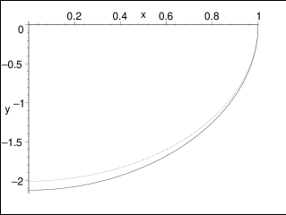
Figure 1: We choose two cases as : $\frac{Q^{2}_{1}}{a^{2}_{0}}=1$ , $\frac{Q^{2}_{2}}{a^{2}_{0}}=2^{2}$, $\frac{P^{2}_{1}}{a^{2}_{0}}=3^{2}$, $\frac{P^{2}_{2}}{a^{2}_{0}}=4^{2}$ (for solid line) and $\frac{Q^{2}_{1}}{a^{2}_{0}}=(.1)^{2}$ , $\frac{Q^{2}_{2}}{a^{2}_{0}}=(.2)^{2}$, $\frac{P^{2}_{1}}{a^{2}_{0}}=(.3)^{2}$, $\frac{P^{2}_{2}}{a^{2}_{0}}=(.4)^{2}$( for dotted line ). We define $\frac{b}{a_{0}}=x$ , $\frac{\Omega}{a_{0}}=y$ and plot y Vs. x . The variation of total amount of exotic matter on the shell with respect to the parameter b is shown in the figure.

If $a_{0},P_{i},Q_{i}>>b$, then

$\Omega=-\frac{1}{2}a_{0}[(a_{0}+{Q_{1}})(a_{0}+{Q_{2}})(a_{0}+{P_{1}})(a_{0}+{P_{2}})]^{\frac{1}{4}}[\frac{1}{(a_{0}+{Q_{1}})}+\frac{1}{(a_{0}+{Q_{2}})}+\frac{1}{(a_{0}+{P_{1}})}+\frac{1}{(a_{0}+{P_{2}})}]$

Also, if one considers, $P_{i}=Q_{i}=Q$, then $\Omega=-2\sqrt{(a_{0}+b)(a_{0}-b)}$.

The variation of $\frac{\Omega}{a_{0}}$ with respect to the parameter $\frac{b}{a_{0}}$ is shown in fig-II.

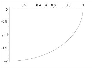
Figure 2: We define $\frac{b}{a_{0}}=x$ , $\frac{\Omega}{a_{0}}=y$ and plot y Vs. x . For the case, $P_{i}=Q_{i}=Q$, the variation of total amount of exotic matter on the shell with respect to the parameter b is shown in the figure.

The above equations describing $\Omega$ indicate that the total amount of exotic matter can be reduced by taking the wormhole radius close to parameter ’b’.

Case-II :

In this case, we shall treat b as a fixed constant. Now,for large Q, the expression of $\Omega$ will take the following form,

$\Omega=-\frac{1}{2}\sqrt{(a_{0}+b)(a_{0}-b)}[\prod{Q^{\frac{1}{4}}}(1+\frac{a_{0}}{4Q}+\frac{4b^{2}-3a_{0}^{2}}{Q^{2}}+0(\frac{1}{Q^{3}}))][\sum(\frac{1}{Q}-\frac{a_{0}}{Q^{2}}+0(\frac{1}{Q^{3}}))]$

The above expression indicates that the total amount of exotic matter will be needed more with the increase of Q. Thus required exotic matter is minimum, when Q takes its minimum values, say $Q=Q_{min}$ .

6. Concluding remarks:

In recent years, string theory has become an active area of research because it generalizes the Einstein theory in many ways. It is of interest to investigate how the properties of black holes are modified when the black holes of the effective four dimensional heterotic string theory compactified on a six torus are considered [14-15]. So black hole solution arising from toroidally compactified heterotic string theory has been an intriguing subject for researchers. In this article we have constructed a new class of thin wormhole by surgically grafting two black hole spacetimes arising from heterotic string theory on a six torus. We have given our attention only how to get the geometry of the thin wormhole. We have analyzed the dynamical stability of the thin shell, considering linearized radial perturbations around stable solution. To analyze this, we define a parameter $\beta^{2}=\frac{p^{\prime}}{\sigma^{\prime}}$ as a parametrization of the stability of equilibrium. We have obtained a restriction on $\beta^{2}$ to get stable equilibrium of the thin wormhole( see eq.(26)). It is shown that the matter within the shell violates the weak energy condition but that matter may obey null energy condition. Although it is not possible to provide the mechanism that provide the exotic matter but rather we have calculated an integral measuring of the total amount of exotic matter. Finally, we have shown that total amount of exotic matter needed to support traversable wormhole can be reduced as desired with the suitable choice of the parameters.

Acknowledgments

F.R. is thankful to Jadavpur University and DST , Government of India for providing financial support under Potential Excellence and Young Scientist scheme . MK has been partially supported by UGC, Government of India under Minor Research Project scheme. We are also grateful to the anonymous referee for his valuable comments and constructive suggestions.

Appendix

$A=5[(\frac{-1}{2(a_{0}+\hat{Q_{1}})^{2}}+\frac{-1}{2(a_{0}+\hat{Q_{2}})^{2}}+\frac{-1}{2(a_{0}+\hat{P_{1}})^{2}}+\frac{-1}{2(a_{0}+\hat{P_{2}})^{2}})+\frac{1}{4}(\frac{1}{(a_{0}+\hat{Q_{1}})}+\frac{1}{(a_{0}+\hat{Q_{2}})}+\frac{1}{(a_{0}+\hat{P_{1}})}+\frac{1}{(a_{0}+\hat{P_{2}})})^{2}][\frac{(a_{0}+b)(a_{0}-b)}{[(a_{0}+\hat{Q_{1}})(a_{0}+\hat{Q_{2}})(a_{0}+\hat{P_{1}})(a_{0}+\hat{P_{2}})]^{\frac{1}{2}}}]$

$B=[\frac{1}{2(a_{0}+\hat{Q_{1}})}+\frac{1}{2(a_{0}+\hat{Q_{2}})}+\frac{1}{2(a_{0}+\hat{P_{1}})}+\frac{1}{2(a_{0}+\hat{P_{2}})}][\frac{2a_{0}}{a_{0}^{2}-b^{2}}-\frac{1}{2}(\frac{1}{(a_{0}+\hat{Q_{1}})}+\frac{1}{(a_{0}+\hat{Q_{2}})}+\frac{1}{(a_{0}+\hat{P_{1}})}+\frac{1}{(a_{0}+\hat{P_{2}})})][\frac{(a_{0}+b)(a_{0}-b)}{[(a_{0}+\hat{Q_{1}})(a_{0}+\hat{Q_{2}})(a_{0}+\hat{P_{1}})(a_{0}+\hat{P_{2}})]^{\frac{1}{2}}}]$

$C=\frac{1}{2}[\frac{2a_{0}}{a_{0}^{2}-b^{2}}-\frac{1}{2}(\frac{1}{(a_{0}+\hat{Q_{1}})}+\frac{1}{(a_{0}+\hat{Q_{2}})}+\frac{1}{(a_{0}+\hat{P_{1}})}+\frac{1}{(a_{0}+\hat{P_{2}})})]^{2}[\frac{(a_{0}+b)(a_{0}-b)}{[(a_{0}+\hat{Q_{1}})(a_{0}+\hat{Q_{2}})(a_{0}+\hat{P_{1}})(a_{0}+\hat{P_{2}})]^{\frac{1}{2}}}]$

$D=\frac{2(a_{0}+b)(a_{0}-b)}{[(a_{0}+\hat{Q_{1}})(a_{0}+\hat{Q_{2}})(a_{0}+\hat{P_{1}})(a_{0}+\hat{P_{2}})]^{\frac{1}{2}}}[(\frac{1}{(a_{0}+\hat{Q_{1}})}+\frac{1}{(a_{0}+\hat{Q_{2}})}+\frac{1}{(a_{0}+\hat{P_{1}})}+\frac{1}{(a_{0}+\hat{P_{2}})})(\frac{1}{4}[\frac{1}{(a_{0}+\hat{Q_{1}})}+\frac{1}{(a_{0}+\hat{Q_{2}})}+\frac{1}{(a_{0}+\hat{P_{1}})}+\frac{1}{(a_{0}+\hat{P_{2}})}]^{2}+\frac{-1}{2(a_{0}+\hat{Q_{1}})^{2}}+\frac{-1}{2(a_{0}+\hat{Q_{2}})^{2}}+\frac{-1}{2(a_{0}+\hat{P_{1}})^{2}}+\frac{-1}{2(a_{0}+\hat{P_{2}})^{2}})+\frac{1}{(a_{0}+\hat{Q_{1}})^{3}}+\frac{1}{(a_{0}+\hat{Q_{2}})^{3}}+\frac{1}{(a_{0}+\hat{P_{1}})^{3}}+\frac{1}{(a_{0}+\hat{P_{2}})^{3}}+(\frac{-1}{2(a_{0}+\hat{Q_{1}})^{2}}+\frac{-1}{2(a_{0}+\hat{Q_{2}})^{2}}+\frac{-1}{2(a_{0}+\hat{P_{1}})^{2}}+\frac{-1}{2(a_{0}+\hat{P_{2}})^{2}})(\frac{1}{(a_{0}+\hat{Q_{1}})}+\frac{1}{(a_{0}+\hat{Q_{2}})}+\frac{1}{(a_{0}+\hat{P_{1}})}+\frac{1}{(a_{0}+\hat{P_{2}})})]$

$E=\frac{[\frac{2a_{0}}{a_{0}^{2}-b^{2}}-\frac{1}{2}(\frac{1}{(a_{0}+\hat{Q_{1}})}+\frac{1}{(a_{0}+\hat{Q_{2}})}+\frac{1}{(a_{0}+\hat{P_{1}})}+\frac{1}{(a_{0}+\hat{P_{2}})})][\frac{(a_{0}+b)(a_{0}-b)}{[(a_{0}+\hat{Q_{1}})(a_{0}+\hat{Q_{2}})(a_{0}+\hat{P_{1}})(a_{0}+\hat{P_{2}})]^{\frac{1}{2}}}]}{(\frac{1}{2(a_{0}+\hat{Q_{1}})}+\frac{1}{2(a_{0}+\hat{Q_{2}})}+\frac{1}{2(a_{0}+\hat{P_{1}})}+\frac{1}{2(a_{0}+\hat{P_{2}})})}[(\frac{-1}{2(a_{0}+\hat{Q_{1}})^{2}}+\frac{-1}{2(a_{0}+\hat{Q_{2}})^{2}}+\frac{-1}{2(a_{0}+\hat{P_{1}})^{2}}+\frac{-1}{2(a_{0}+\hat{P_{2}})^{2}})+\frac{1}{4}(\frac{1}{(a_{0}+\hat{Q_{1}})}+\frac{1}{(a_{0}+\hat{Q_{2}})}+\frac{1}{(a_{0}+\hat{P_{1}})}+\frac{1}{(a_{0}+\hat{P_{2}})})^{2}]$

$G=3[\frac{1}{2(a_{0}+\hat{Q_{1}})}+\frac{1}{2(a_{0}+\hat{Q_{2}})}+\frac{1}{2(a_{0}+\hat{P_{1}})}+\frac{1}{2(a_{0}+\hat{P_{2}})}]^{2}[\frac{(a_{0}+b)(a_{0}-b)}{[(a_{0}+\hat{Q_{1}})(a_{0}+\hat{Q_{2}})(a_{0}+\hat{P_{1}})(a_{0}+\hat{P_{2}})]^{\frac{1}{2}}}]$

$H=[\frac{(a_{0}+b)(a_{0}-b)}{[(a_{0}+\hat{Q_{1}})(a_{0}+\hat{Q_{2}})(a_{0}+\hat{P_{1}})(a_{0}+\hat{P_{2}})]^{\frac{1}{2}}}][(\frac{2a_{0}}{a_{0}^{2}-b^{2}}-\frac{1}{2}(\frac{1}{(a_{0}+\hat{Q_{1}})}+\frac{1}{(a_{0}+\hat{Q_{2}})}+\frac{1}{(a_{0}+\hat{P_{1}})}+\frac{1}{(a_{0}+\hat{P_{2}})}))^{2}-\frac{1}{(a_{0}+b)^{2}}-\frac{1}{(a_{0}-b)^{2}}+\frac{1}{2}(\frac{1}{(a_{0}+\hat{Q_{1}})^{2}}+\frac{1}{(a_{0}+\hat{Q_{2}})^{2}}+\frac{1}{(a_{0}+\hat{P_{1}})^{2}}+\frac{1}{(a_{0}+\hat{P_{2}})^{2}})]$

$M=2[(\frac{-1}{2(a_{0}+\hat{Q_{1}})^{2}}+\frac{-1}{2(a_{0}+\hat{Q_{2}})^{2}}+\frac{-1}{2(a_{0}+\hat{P_{1}})^{2}}+\frac{-1}{2(a_{0}+\hat{P_{2}})^{2}})+\frac{1}{4}(\frac{1}{(a_{0}+\hat{Q_{1}})}+\frac{1}{(a_{0}+\hat{Q_{2}})}+\frac{1}{(a_{0}+\hat{P_{1}})}+\frac{1}{(a_{0}+\hat{P_{2}})})^{2}]\sqrt{[\frac{(a_{0}+b)(a_{0}-b)}{[(a_{0}+\hat{Q_{1}})(a_{0}+\hat{Q_{2}})(a_{0}+\hat{P_{1}})(a_{0}+\hat{P_{2}})]^{\frac{1}{2}}}]}[\frac{1}{2(a_{0}+\hat{Q_{1}})}+\frac{1}{2(a_{0}+\hat{Q_{2}})}+\frac{1}{2(a_{0}+\hat{P_{1}})}+\frac{1}{2(a_{0}+\hat{P_{2}})}]$

$N=\sqrt{[\frac{(a_{0}+b)(a_{0}-b)}{[(a_{0}+\hat{Q_{1}})(a_{0}+\hat{Q_{2}})(a_{0}+\hat{P_{1}})(a_{0}+\hat{P_{2}})]^{\frac{1}{2}}}]}[\frac{2a_{0}}{a_{0}^{2}-b^{2}}-\frac{1}{2}(\frac{1}{(a_{0}+\hat{Q_{1}})}+\frac{1}{(a_{0}+\hat{Q_{2}})}+\frac{1}{(a_{0}+\hat{P_{1}})}+\frac{1}{(a_{0}+\hat{P_{2}})})][\frac{1}{2(a_{0}+\hat{Q_{1}})}+\frac{1}{2(a_{0}+\hat{Q_{2}})}+\frac{1}{2(a_{0}+\hat{P_{1}})}+\frac{1}{2(a_{0}+\hat{P_{2}})}]^{2}$

$L=[\frac{1}{2(a_{0}+\hat{Q_{1}})}+\frac{1}{2(a_{0}+\hat{Q_{2}})}+\frac{1}{2(a_{0}+\hat{P_{1}})}+\frac{1}{2(a_{0}+\hat{P_{2}})}]^{3}\sqrt{[\frac{(a_{0}+b)(a_{0}-b)}{[(a_{0}+\hat{Q_{1}})(a_{0}+\hat{Q_{2}})(a_{0}+\hat{P_{1}})(a_{0}+\hat{P_{2}})]^{\frac{1}{2}}}]}$

References

[1] M Visser, Nucl.Phys.B 328, 203 (1989)
[2] W Israel, Nuovo Cimento 44B , 1 (1966) ; erratum -
ibid. 48B, 463 (1967)
[3] E Poisson and M Visser,
Phys.Rev.D 52, 7318 (1995) [arXiv: gr-qc / 9506083]
[4] M Ishak and K Lake, Phys.Rev.D 65, 044011 (2002)
[5] E Eiroa and G Romero,
Gen.Rel.Grav. 36, 651 (2004)[arXiv: gr-qc / 0303093]
[6] F Lobo and P Crawford, Class.Quan.Grav. 21,
391 (2004)
[7] E Eiroa and C Simeone, Phys.Rev.D 70, 044008
(2004)
[8] E Eiroa and C Simeone, Phys.Rev.D 71, 127501 (2005) [arXiv: gr-qc
/ 0502073]
[9] M Thibeault , C Simeone and E Eiroa, gr-qc /
0512029
[10] F Rahaman, M Kalam and S Chakraborty, gr-qc/ 0607061
[11] D Jatkar, S Mukherji and S Panda, Nucl. Phys. B 484,
223 ( 1997)
[12] M Cvetic and D Youm, Nucl. Phys. B 472,
249 ( 1996)
[13] P Mitra,
Phys.Rev.D 57, 7369(1998)
[14] A Sen, Nucl.Phys.B 440, 421 (1995)
[15] M Cvetic and D Youm, Phys.Rev.D 53,
R584 ( 1996)