Frankenstein’s Glue:
Transition functions for approximate solutions

Abstract

Approximations are commonly employed to find approximate solutions to the Einstein equations. These solutions, however, are usually only valid in some specific spacetime region. A global solution can be constructed by gluing approximate solutions together, but this procedure is difficult because discontinuities can arise, leading to large violations of the Einstein equations. In this paper, we provide an attempt to formalize this gluing scheme by studying transition functions that join approximate analytic solutions together. In particular, we propose certain sufficient conditions on these functions and proof that these conditions guarantee that the joined solution still satisfies the Einstein equations analytically to the same order as the approximate ones. An example is also provided for a binary system of non-spinning black holes, where the approximate solutions are taken to be given by a post-Newtonian expansion and a perturbed Schwarzschild solution. For this specific case, we show that if the transition functions satisfy the proposed conditions, the joined solution does not contain any violations to the Einstein equations larger than those already inherent in the approximations. We further show that if these functions violate the proposed conditions, then the matter content of the spacetime is modified by the introduction of a matter-shell, whose stress-energy tensor depends on derivatives of these functions.

1 Introduction

The detection and modeling of gravitational radiation is currently one of the primary driving forces in classical general relativity due to the advent of ground-based [1, 2, 3, 4] and space-born detectors [5, 6]. This radiation is generated in highly dynamical spacetimes, whose exact metric has not yet been found. Approximate solutions to the Einstein equations, both analytical (such as post-Newtonian solutions [7]) and numerical, have served to provide insight on the dynamics of such spacetimes and the character of the radiation produced. These approximations, however, have inherent uncontrolled remainders, or errors, due to truncation of certain higher order terms in the analytical case, or discretization error in the numerical case. An approximate global solution, then, could be constructed by joining several approximate solutions together in some overlap region [8, 9].

Before proceeding, we must distinguish between two different kinds of joined solutions: mixed ones, where one joins an analytical solution to a numerical one; and pure ones, where one joins two analytical solutions that have different but overlapping regions of validity. A special kind of mixed joined solutions have been created in the context of the effective-one-body formalism [10, 11], with the motivation of providing accurate waveform templates to gravitational wave interferometers. Pure joined solutions have been discussed in the context of asymptotic matching, where one of the motivations is to use the joined solution as initial data for relativistic simulations [8, 9]. In this paper, we concentrate on pure joined solutions, although the methods and conditions we find can be straightforwardly extended to mixed joined solutions.

The construction of pure joined solutions is not always simple because approximation methods tend to break down in highly dynamical spacetimes. The main difficulty lies in that approximate solutions usually depend on the existence of a background about which to perturb the solution. However, in highly dynamical spacetimes, such a background cannot usually be constructed. Thus, in those scenarios, the region of validity of the different approximations tends not to overlap. In slightly less dynamical cases, the regions of validity can overlap, but the different approximate metrics usually describe the spacetime in different coordinates and parameters. Patching [12] could be used to relate the different approximate solutions, but this method usually leads to an overdetermined system if we require the patched metric to be differentiable at the junction. A better alternative is to relate the approximate solutions via asymptotic matching, which guarantees that adjacent metrics and their derivatives be asymptotic to each other in some overlap region.

Asymptotic matching was developed as a technique of multiple-scale analysis to solve non-linear partial differential equations [12, 13]. In general relativity, this method was first studied in [14, 15, 16, 17, 18] and it has recently had important applications to post-Newtonian theory [7], black hole perturbation theory [19] and initial data constructions [8, 9]. Asymptotic matching requires that we compare the asymptotic expansions of the approximate solutions inside the region of the manifold where the regions of validity of the approximations overlap (the buffer zone.) This method then provides a coordinate and parameter transformation that relates the approximate metrics, such that adjacent metrics and their derivatives become asymptotic to each other inside the buffer zone. In essence, asymptotically matched approximations are guaranteed to represent the same metric components in the same coordinate system inside the buffer zone.

After matching has been carried out, there is still freedom as to how to join the matched approximate solutions together. The simplest way to do so is through a weighted linear combination of approximate solutions with transition functions. This method was first considered in depth in [8, 9], where a binary black hole system was studied to construct initial data for numerical simulations (the so-called Frankenstein approach). In that work, only broad comments were made as to the type of allowed transition functions, requiring only that the functions be “differentiable enough,” and the the properties and conditions these functions must satisfy were not studied. A priori, it might not be clear which functions are allowed such that the global metric still approximately solves the Einstein equations. For instance, it might seem natural to use Heaviside functions to join the metrics together at a hypersurface, as is done in the standard junction conditions of general relativity [20, 21, 22, 23, 24, 25, 26, 27, 28]. These joining procedure works well when dealing with exact solutions to the Einstein equations, in the sense that the joined solution is itself also a solution. As we show in this paper, however, when working with approximate solutions better transition functions need to be found.

The purpose of this paper is to study whether a global approximate solution to the Einstein equations, be it pure or mixed, can be constructed directly from a weighted linear superposition of approximate solutions with transition functions. We thus refine, prove and verify many of the broad statements made in [8, 9] regarding transition functions. This goal is achieved by constraining the family of allowed transition functions for pure joined solutions via certain sufficient asymptotic differentiability conditions. These conditions are independent of the perturbative order to which asymptotic matching is carried out and the location in which the transition occurs, as long as it is inside the buffer zone. We then derive and prove theorems that guarantee that pure joined solutions constructed with this restricted family of transition functions satisfy the Einstein equations to the same order as the approximations. Moreover, we also show that if the transition functions do not satisfy the proposed conditions, their derivatives modify the energy-matter content of the spacetime by introducing a non-negligible stress-energy tensor. Finally, we extend these theorems to solutions projected onto spatial hypersurfaces, so that they can be directly applied to initial data construction schemes. These theorems then allow for the systematic construction of pure joined solutions and they can be straightforwardly extended to mixed joined solutions.

An example of the proposed theorems and allowed transition functions is then provided by studying a binary system of non-spinning black holes, where the approximate solutions are taken to be given by a post-Newtonian expansion and a linearly perturbed Schwarzschild solution. We shall not perform a systematic study of transition functions here, but instead we pick functions that are variations of those chosen in [8, 9] in order to illustrate how the gluing procedure works and how it breaks down. We explicitly show that if the transition functions satisfy the proposed conditions, the $4$-Ricci scalar calculated with the pure joined solution vanishes to the same order as the uncontrolled remainders in the approximations. In particular, we explicitly show that derivatives of the pure joined approximate solution built with appropriate transition functions are equal to derivatives of both original approximate solutions up to the uncontrolled remainders in the approximations. We also numerically show that if the transition functions violate the proposed conditions, their derivatives modify the matter content of the spacetime by introducing a shell of matter. In this manner, we explicitly verify, both analytically and numerically, that a pure joined solution does represent the same spacetime as that of the original approximate solutions in their respective regions of validity up to the accuracy of the approximations used.

This paper is divided as follows: in section 2 we review the standard junction conditions at a hypersurface, so that we can extend them to the case where the solutions used are approximate instead of exact, provided the existence of a buffer zone; in section 3 we study how to join approximate solutions with transition function and derive conditions such that a pure joined solution satisfies the Einstein equations to the same order as the approximations used; in this section, we also study projections of these pure joined solutions to a Cauchy hypersurface in order to develop conditions for transition functions that can be used in initial data construction schemes; in section 4 we study an example of the theorems formulated by considering a binary system of non-spinning black hole, constructing approximate global metrics with different transition function, and explicitly calculating the $4$-Ricci scalar; in section 5 we conclude and point to future research.

The notation of this paper is as follows: Greek indices range over all spacetime indices, while Latin indices range only over spatial indices; the symbol ${\cal{O}}(A)$ stands for terms of order $A$ at most, while the symbol ${\cal{O}}(A,B)$ stands for remainders of order $A$ or $B$ at most, where $A$ and $B$ are dimensionless; a tilde superscript $\widetilde{A}$ stands for the asymptotic expansion of $A$ as defined in [12, 13]; the relation $A=B+{\cal{O}}(C)$ means that $A$ is asymptotic to $B$ with uncontrolled remainders of order $C$ (the so-called Landau or asymptotic notation); we use units where $c=G=1$. Symbolic calculations are performed with either Mathematica or Maple.

2 Junction Conditions at a Hypersurface

In this section, we review a variation of the standard junction conditions of general relativity. These conditions have been discussed extensively in the literature (see [20, 21, 22, 23, 24, 25, 26, 27, 28] and references therein.) Here, we review only those concepts important to the understanding of this paper, following in particular [28]. Certain departures from the notation of [28] are so that the generalization to the case of approximate solutions in the next section becomes easier.

Let us first set up the problem. Consider a spatial (or timelike) hypersurface $\cal{J}$ that divides spacetime into two regions: ${\cal{C}}_{1}$ and ${\cal{C}}_{2}$. Each of these regions possesses an associated metric and coordinates, $\{g_{\mu\nu}^{(1)},x_{(1)}^{\alpha}\}$ and $\{g_{\mu\nu}^{(2)},x_{(2)}^{\alpha}\}$, such that these metrics solve the Einstein equations exactly in their respective regions. In the literature, this exact solutions and coordinate systems are also sometimes referred to as $\{g_{\mu\mu}^{\pm},x_{\pm}^{\alpha}\}$. Let us further assume that an overlapping coordinate system $x^{\alpha}$ exists in a neighbourhood of ${\cal{J}}$. The problem is to formulate junction conditions on ${\cal{J}}$ that guarantee that the joined $4$-metric satisfies the Einstein equations.

Let us make these statements more precise by considering a congruence of geodesics piercing ${\cal{J}}$ defined with respect to first metric in ${\cal{C}}_{1}$ and the second metric in ${\cal{C}}_{2}$ (see [28] for a detailed definition of such congruence.) Let then $\ell$ denote the proper time (or proper distance) along the geodesics, such that $\ell=0$ corresponds to when the geodesics reach ${\cal{J}}$. The joined solution then takes the following form [28]:

$$g_{\mu\nu}=\Theta(\ell)g_{\mu\nu}^{(1)}+\Theta(-\ell)g_{\mu\nu}^{(2)},$$ (1)

where $\Theta(\cdot)$ is the Heaviside function. Equation (1) implicitly uses coordinates $x^{\alpha}$ that overlap both the coordinates local to ${\cal{C}}_{1}$ and ${\cal{C}}_{2}$ in a neighbourhood of ${\cal{J}}$.

We now proceed to formulate the junction conditions. The first junction condition arises by requiring that the $4$-metric be continuous across ${\cal{J}}$, in a coordinate system $x^{\alpha}$ that overlaps both $x^{\alpha}_{1}$ and $x^{\alpha}_{2}$ in an open region that contains this hypersurface. This condition can be expressed in a coordinate-independent way by projecting it to ${\cal{J}}$. Then, in terms of $3$-tensors this condition becomes

$$\left.h_{ab}^{(1)}\right|_{{\cal{J}}}=\left.h_{ab}^{(2)}\right|_{{\cal{J}}},$$ (2)

where here $h_{ab}$ is the $3$-metric associated with the junction hypersurface, i.e.

$$h_{\mu\nu}=g_{\mu\nu}+e_{\pm}n_{\mu}n_{\nu},$$ (3)

with $n_{a}$ normal to ${\cal{J}}$ and $e_{\pm}=\pm 1$ depending on whether ${\cal{J}}$ is spatial ($-$) or timelike ($+$.) Equation (2) guarantees that the hypersurface ${\cal{J}}$ has a well-defined geometry. These equations also imply that the metric is differentiable across ${\cal{J}}$, except for its normal derivative to ${\cal{J}}$ that in general is discontinuous.

The second junction condition arises by requiring that this normal derivative does not lead to violations of the Einstein equations across ${\cal{J}}$. In terms of $3$-tensors on ${\cal{J}}$, this condition becomes

$$\left.K_{ab}^{(1)}\right|_{{\cal{J}}}=\left.K_{ab}^{(2)}\right|_{{\cal{J}}}.$$ (4)

One can show that the failure of these equations to be satisfied changes the distribution of energy-momentum tensor of the spacetime and gives raise to a shell of matter with stress-energy tensor [28]

$$S_{ab}=-\frac{\epsilon}{8\pi}\left[\left.K_{ab}^{(1)}\right|_{\cal{J}}-\left.K_{ab}^{(2)}\right|_{\cal{J}}-h_{ab}\left(\left.K^{(1)}\right|_{\cal{J}}-\left.K^{(2)}\right|_{\cal{J}}\right)\right].$$ (5)

In the next section, we shall be mostly interested in vacuum spacetimes, for which such a stress-energy tensor should vanish.

The satisfaction of the Einstein equations out of ${\cal{J}}$ by (1) and the absence of a stress-energy tensor as in (5) then guarantees that the junction conditions [(2) and (4)] are also satisfied. Exact solutions, however, are rarely available for astrophysically realistic scenarios. In that case, one must rely on approximate solutions, for which similar conditions to those discussed here can be found, as we shall study in the next section.

3 Pure joined solutions

In this section we build a pure joined solution by extending the standard junction conditions to the case where the metrics $g_{\mu\nu}^{(1,2)}$ are only approximate solutions to the Einstein equations. For simplicity, we assume a vacuum spacetime and that there exists analytic approximate expressions for $g_{\mu\nu}^{(1,2)}$, such that pure joined solutions are sought. The conclusions of this section, however, can straightforwardly be extended to other cases, where numerical solutions are available instead of analytical ones, provided information about first and second derivatives of the numerical solutions is also available (note that for numerical solutions the continuum derivative operator must be replaced by its finite counterpart.) As shown in [8, 9], the first step in joining approximate solutions is to apply asymptotic matching inside some overlap region. Once this has been done, one can search for conditions such that the pure joined metric tensor satisfies the Einstein equations to the same order as $g_{\mu\nu}^{(1,2)}$. We here first present the basics of asymptotic matching as applicable to this problem [7, 8]. We then search for asymptotic junction conditions (or buffer zone conditions), which are asymptotic in the sense of [12, 13] and, thus, are to be understood only approximately to within some uncontrolled remainder.

3.1 Asymptotically matched metrics

Consider then a manifold ${\cal{M}}$ that can be divided into two submanifolds with boundary $C_{1}$ and $C_{2}$, each equipped with a approximate metrics $g_{\mu\nu}^{(1)}$ and $g_{\bar{\mu}\bar{\nu}}^{(2)}$ and a coordinate system $x^{\alpha}$ and $x^{\bar{\alpha}}$ respectively. These metrics are approximate in the sense that they solve the Einstein equations to ${\cal{O}}(\epsilon_{n}^{\ell_{n}})$ for some $l\in\mathbb{N}$ in their respective submanifolds, e.g. in vacuum

$$G_{\mu\nu}[g_{\mu\nu}^{(n)}]={\cal{O}}(\epsilon_{n}^{\ell_{n}+1}),$$ (6)

where $n=\{1,2\}$, $(\ell_{1},\ell_{2})$ are real numbers greater than zero, and $\epsilon_{n}\ll 1$ is some dimensionless combination of parameters and coordinates relative to the $n$-th submanifold. The symbol ${\cal{O}}(\epsilon_{n}^{\ell_{n}+1})$ refers to terms of relative order $\epsilon_{n}^{\ell_{n}+1}$ with respect to the leading order term in the approximate solution $g_{\mu\nu}^{(n)}$. In principle, there could be logarithms of $\epsilon_{n}$ present in the remainders, such as in high-order post-Newtonian expansions, but we neglect such terms here because they shall not affect the analysis of this paper. Notice that we use here bars to denote the different coordinate systems (as opposed to numbers, as in the previous section) because we must be more careful about the coordinates used in these approximate metric components. For concreteness, let the region of validity of $g_{\mu\nu}^{(1)}(x^{\alpha})$ be defined by $x^{\alpha}\gg x^{\alpha}_{in}$ and that of $g_{\mu\nu}^{(2)}(x^{\bar{\alpha}})$ by $x^{\bar{\alpha}}\ll x^{\bar{\alpha}}_{out}$. These inequalities define a spacetime region of validity, since the approximate metric might not be valid for all times. For example, such is the case for the post-Newtonian metric of two point particles in quasi-circular orbit, which is valid only for times $t\ll t_{c}$, where $t_{c}$ is the time of coalescence.

Let us further assume that these submanifolds overlap in some $4$-volume, defined by the intersection ${\cal{B}}=C_{1}\cap C_{2}$, and sometimes referred to as the overlap region or buffer zone. The boundary of the buffer zone, $\partial{\cal{B}}$, cannot be determined exactly, because it is inherently tied to the regions of validity of the approximate solutions, which themselves are only defined approximately. With this in mind, let us further assume that the charts $\{x^{\alpha}\}$ and $\{x^{\bar{\alpha}}\}$ are defined in the neighbourhood of any field point in the buffer zone and that they satisfy $x^{\bar{\alpha}}=x^{\alpha}+{\cal{O}}(\epsilon_{1}^{\ell_{1}+1},\epsilon_{2}^{\ell_{2}+1})$. The buffer zone can then be asymptotically defined by the following condition: $(x^{\alpha}_{in}x_{\alpha}^{in})^{1/2}\ll(x^{\alpha}x_{\alpha})^{1/2}\ll(x^{\alpha}_{out}x_{\alpha}^{out})^{1/2}$, where indeces are raised or lowered with the local metric to ${\cal{C}}_{1,2}$. Wherever possible, we use the Landau notation, which specifically specifies the behavior of the remainder. The definition of the boundary of the buffer zone should be understood only in an asymptotic sense, as defined in [12, 13]. This boundary is made up of two disconnected pieces, $\partial{\cal{B}}_{-}$ and $\partial{\cal{B}}_{+}$, defined via $x^{\alpha}=x_{in}^{\alpha}+{\cal{O}}(\epsilon_{1}^{\ell_{1}+1},\epsilon_{2}^{\ell_{2}+1})$ and $x^{\alpha}=x_{out}^{\alpha}+{\cal{O}}(\epsilon_{1}^{\ell_{1}+1},\epsilon_{2}^{\ell_{2}+1})$ respectively. The definition of the buffer zone can be thought of in terms of a simplistic spherically symmetric static example, where $x^{\alpha}\to r$, $\partial{\cal{B}}$ is a spherical shell and $\partial{\cal{B}}_{\pm}$ are $2$-spheres. However, in practical examples, such as binary black hole spacetimes, the boundary of the buffer zone is not simply a spherical shell, but instead it acquires some deformation in accordance with the deformation of the spacetime that is being modeled.

Before proceeding with the description of asymptotic matching, let us make some comments on the approach adopted in this paper. In the previous paragraphs and in what shall follow, we have not adopted a rigorous geometrical approach in the description of asymptotic matching, the definition of the buffer zone and the submanifolds. A rigorous geometrical approach, for example, would impose other constraints on ${\cal{B}}$, such that it is properly embedded in ${\cal{C}}_{1}$ and ${\cal{C}}_{2}$. Furthermore, such an approach would describe the conditions under which asymptotic matching can be performed, since in general this method is valid only locally. Instead of such an approach, in this paper we adopt an analytical one, where we only provide a minimal amount of details in order to make the presentation simpler. For example, we shall restrict our attention to coordinate grids that coincide when both $\epsilon_{1}\to 0$ and $\epsilon_{2}\to 0$ and, henceforth, we shall call ${\cal{C}}_{1,2}$ regions instead of submanifolds. Such an approach is adopted because the aim of this paper is not to provide a detailed geometrical account of asymptotic matching, but instead to study transition functions and approximate joined solutions (see [29] and references therein for a more detailed and rigorous geometric account of asymptotic matching.)

The approximate metrics live in different regions and depend on different coordinates ($x^{\alpha}$,$x^{\bar{\alpha}}$) and local parameters ($\theta^{\alpha}$,$\theta^{\bar{\alpha}}$.) Examples of these parameters are the mass of the system and its velocity. However, since both $g_{\mu\nu}^{(n)}$ are valid in ${\cal{B}}$, both coordinate systems must be valid in the buffer zone (i.e., the charts of $C_{n}$ overlap in ${\cal{B}}$.) Using the uniqueness theorems of asymptotic expansions [12, 13], one can find a coordinate and parameter transformation to relate adjacent regions inside ${\cal{B}}$. In order to achieve this, one must first compute the asymptotic expansions of the approximate line elements, $\widetilde{ds}^{2}_{(n)}$, near the boundaries of the buffer zone, $\partial{\cal{B}}$, and then compare them inside ${\cal{B}}$ but yet away from $\partial{\cal{B}}$, i.e.

$$\widetilde{ds}^{2}_{(1)}-\widetilde{ds}^{2}_{(2)}={\cal{O}}(\epsilon_{1}^{\ell_{1}+1},\epsilon_{2}^{\ell_{2}+1}),\qquad\textrm{\mbox{in}}\quad{\cal{B}}\;\backslash\;{\partial{\cal{B}}},$$ (7)

where the $\backslash$ symbol is the standard exclusion symbol of set theory and where ${\cal{O}}(\epsilon_{1}^{\ell_{1}+1},\epsilon_{2}^{\ell_{2}+1})$ stands for uncontrolled remainders of order $\epsilon_{1}^{\ell_{1}+1}$ or $\epsilon_{2}^{\ell_{2}+1}$ as defined at the end of Sec. 1. Using (7), a coordinate transformation $\psi:x^{\bar{\alpha}}\to x^{\alpha}$ and a parameter transformation $\phi:\theta^{\bar{\alpha}}\to\theta^{\alpha}$ can be found inside ${\cal{B}}$. We have written (7) in terms of the line element, but we could have easily written it in terms of the metric components. In fact, depending on the calculation, it might be necessary to asymptotically match different components of the metric to different order. For example, for the construction of initial data, the $g_{00}$ and $g_{ij}$ components of the metric need to be matched to lower order than the $g_{0i}$ components [8, 9]. In what follows, we will assume that all metric components have been asymptotically matched to the same order. When this is not the case, the conditions that we shall propose on transition functions can be adapted by noting that one must use the highest order to which metric components have been asymptotically matched.

These transformations guarantee that all components of adjacent $4$-metrics are asymptotic to each other inside the buffer zone [12, 13]. This fact implies that the derivatives of adjacent metrics are also asymptotic to each other

$$\frac{\partial^{m}}{\partial x^{\alpha_{1}}\ldots\partial x^{\alpha_{m}}}g_{\mu\nu}^{(1)}-\frac{\partial^{m}}{\partial x^{\alpha_{1}}\ldots\partial x^{\alpha_{m}}}g_{\mu\nu}^{(2)}={\cal{O}}(\epsilon_{1}^{\ell_{1}+1-m},\epsilon_{2}^{\ell_{2}+1-m}),$$ (8)

for all $m<l$. However, the relative order to which the derivatives of adjacent metrics are asymptotic to each other is in general not the same as the relative order to which the adjacent metrics themselves are asymptotic to each other. This reduction in matching accuracy is due to the implicit assumption that asymptotic matching is carried out to some finite order. In (8), we have assumed that this decrease in accuracy occurs in single powers of $\epsilon_{1,2}$, but if this is not the case the results of this paper can be rescaled appropriately.

Let us provide a general example of such matching accuracy reduction, without specifying a particular spacetime (for a more detailed example see [8, 9].) Consider a post-Newtonian expression that is known to ${\cal{O}}(1/c^{4})$ and that is asymptotically matched to a perturbed black hole solution in some buffer zone to ${\cal{O}}(1/c^{4},\epsilon^{2})$, where $c$ is here the speed of light and $\epsilon$ is the black hole perturbation theory expansion parameter. Let us now take the time derivative of the post-Newtonian expression, which results in a term of ${\cal{O}}(1/c^{5})$. In post-Newtonian theory, one would never truncate the differentiated term at ${\cal{O}}(1/c^{4})$. However, in the theory of asymptotic matching to a finite order, the time derivative of the post-Newtonian quantity remains matched only to ${\cal{O}}(1/c^{4},\epsilon^{2})$, and thus it will disagree with the perturbed black hole quantity at ${\cal{O}}(1/c^{5})$. It is in this sense that differentiation usually decreases the relative order to which two expression have been asymptotically matched (we should note that when asymptotic matching is carried out to all orders, then this reduction in matching accuracy disappears [29].)

Let us provide a more explicit example that, although similar in spirit to the one described above, does not require general relativity. Consider two functions

$$f(t)=\left[f_{0}^{2}+2f_{1}^{2}\epsilon_{1}x(\omega\;t)\right]^{1/2},\qquad g(t)=\frac{9}{9+\epsilon_{2}y(\Omega\;t)},$$ (9)

where $f_{0,1}$ are constants and $x(\omega t)$ and $y(\Omega t)$ are periodic funtions of time with period $1/\omega$ and $1/\Omega$ respectively. Let us pretend that $f(t)$ and $g(t)$ are approximate solutions to the same differential equation in the limits $\epsilon_{1}\ll 1$ and $\epsilon_{2}\ll 1$ respectively. If we asymptotically match these functions in a buffer zone where both $\epsilon_{1}\ll 1$ and $\epsilon_{2}\ll 1$ up to uncontrolled remainders of ${\cal{O}}(\epsilon_{1}^{2},\epsilon_{2}^{2})$, we discover that at $t=0$ the constants are $f_{0}=1$ and $f_{1}=y(0)/[9x(0)]$. If we now study their time derivatives, we find that at $t=0$

$$\frac{\partial f}{\partial t}=\epsilon_{1}\frac{y(0)}{9x(0)}\omega\left(\frac{\partial x}{\partial t}\right)_{t=0},\qquad\frac{\partial g}{\partial t}=\frac{\epsilon_{2}}{9}\Omega\left(\frac{\partial y}{\partial t}\right)_{t=0},$$ (10)

with uncontrolled remainders of ${\cal{O}}(\epsilon_{1}^{2},\epsilon_{2}^{2})$. Note that the derivatives are not equal to each other to this order because the velocities $\omega$ and $\Omega$ have not yet been determined via asymptotic matching. The reduction in matching accuracy is here explicit since, while $f(t)$ and $g(t)$ have been asymptotically matched up to uncontrolled remainders of ${\cal{O}}(\epsilon_{1}^{2},\epsilon_{2}^{2})$, their time derivatives match only up to uncontrolled remainders of ${\cal{O}}(\epsilon_{1},\epsilon_{2})$.

Henceforth, we assume that asymptotic matching has been carried out and that one of the metrics has been transformed according to $\{\psi,\phi\}$ such that (7) holds. We refer the reader to [12, 13] for more details on the theory of asymptotic analysis and [7, 8, 14, 15, 16, 17, 18] for a more detailed discussion on asymptotic expansions in general relativity.

3.2 Asymptotic Junction Conditions

Let us now return to the buffer zone and note that it can be foliated by a family of junction hypersurfaces ${\cal{J}}_{i}$, where $i$ labels the member of the family. For simplicity, we choose these hypersurfaces to be timelike, since in the next section we project the $4$-metric to a Cauchy (spatial) hypersurface $\Sigma$ and it is convenient then that ${\cal{J}}_{i}$ be orthogonal to $\Sigma$. Asymptotic matching has provided a coordinate transformation to relate the charts inside ${\cal{B}}$, so, in particular, these matched coordinates are valid in an open region containing every ${\cal{J}}_{i}$ as long as this is not close to ${\partial{\cal{B}}}$. We look for asymptotic junction conditions in this subregion of ${\cal{B}}$ (i.e. away from ${\partial{\cal{B}}}$), in terms of differentiability conditions of $g_{\mu\nu}^{(n)}$.

Furthermore, let us also consider a family of geodesic congruences $\gamma_{i}$ that pierce ${\cal{J}}_{i}$. The $i$th member of the family is parameterized by proper distance $\ell_{i}$ to the $i$th hypersurface ${\cal{J}}_{i}$, such that $\ell_{i}=0$ occurs when that member reaches that hypersurface. Such a family of geodesic congruences is defined with respect to the approximate metrics $g_{\mu\nu}^{(n)}$ since these metrics are equal to each other up to uncontrolled remainders in the asymptotic matching scheme. Even though these geodesics are not strictly necessary for the construction of asymptotic junction conditions, we find them useful to define a measure of distance to ${\cal{J}}_{i}$, which shall later become important in the definition of transition functions.

We can now begin to look for asymptotic junction conditions by considering the following $4$-metric tensor:

$$g_{\mu\nu}=F(\ell_{i})\;g_{\mu\nu}^{(1)}+\left[1-F(\ell_{i})\right]\;g_{\mu\nu}^{(2)},$$ (11)

where $F(\cdot)$ is a (proper) transition function that smoothly ranges from zero to unity inside ${\cal{B}}$ and which will be defined more rigorously later. Equation (11) is motivated by the fact that any tensor $E^{a_{1}a_{2}\ldots a_{i}}{}_{b_{1}b_{2}\ldots b_{j}}$ can always be split into

$$E^{a_{1}a_{2}\ldots a_{i}}{}_{b_{1}b_{2}\ldots b_{j}} = G^{a_{1}a_{2}\ldots a_{i}}{}_{b_{1}b_{2}\ldots b_{j}}F(\ell_{i})$$ (12)

$$+ \left[1-F(\ell_{i})\right]H^{a_{1}a_{2}\ldots a_{i}}{}_{b_{1}b_{2}\ldots b_{j}},$$

provided that

$$E^{a_{1}a_{2}\ldots a_{i}}{}_{b_{1}b_{2}\ldots b_{j}}=G^{a_{1}a_{2}\ldots a_{i}}{}_{b_{1}b_{2}\ldots b_{j}}=H^{a_{1}a_{2}\ldots a_{i}}{}_{b_{1}b_{2}\ldots b_{j}}$$ (13)

inside the transition region and that the proper transition function is sufficiently regular. The regularity requirement is to guarantee that both terms of (12) are differentiable. In (11) this split is valid because $g_{\mu\nu}^{(1)}$ is asymptotic to $g_{\mu\nu}^{(2)}$ in ${\cal{B}}$ up to uncontrolled remainders once the maps $\{\psi,\phi\}$ have been applied. As we will see below, however, care must be taken when constructing such proper transition functions $F(\cdot)$ to avoid ruining the differentiability properties of the joined metric.

Let us now define proper transition functions in order to clarify how to merge the metrics via (11). A proper transition function is a smooth real map ${\cal{F}}:\Re\to\left[0,1\right]$ that ranges from zero to unity inside some transition window $w$, while it acquires the value of $1/2$ as $\ell_{i}\to 0$, and that satisfies the following conditions:

$$F(\ell_{i}) \to 1\quad{\textrm{as}}\quad\ell_{i}\to\ell_{+},$$

$$F(\ell_{i}) \to 0\quad{\textrm{as}}\quad\ell_{i}\to\ell_{-},$$ (14)

where here $\ell_{\pm}$ is the proper distance to $\partial{\cal{B}}_{\pm}$. Note that the point $\ell_{i}=0$ is where the global approximate metric of (11) contains equal contributions from $g_{\mu\nu}^{(1)}$ and $g_{\mu\nu}^{(2)}$. The transition window will be studied later in Sec. 4, but we can think of it qualitatively as a parameter of a proper transition function that determines the region where these functions are significantly different from unity or zero. The requirement that a proper transition function vanishes or tends to unity at $\partial{\cal{B}}_{\pm}$ is necessary to avoid contamination of $g_{\mu\nu}^{(1)}$ in ${\cal{C}}_{2}$ and vice versa, since in general $g_{\mu\nu}^{(n)}$ has large uncontrolled remainders and could diverge outside its region of validity. In fact, the speed at which a proper transition function must tend to unity or zero will depend on the speed of the growth of the uncontrolled remainders of the approximations outside their region of validity, as we shall study later. This definition does not constrain how the transition function behaves inside the transition region. Also note that this family of functions tends to the Heaviside function of the previous section as $w\to 0$ and that it does not need to be analytic. We shall not constrain this family further for now, but instead we search for conditions on this family such that (11) satisfies the Einstein equations to the same order as $g_{\mu\nu}^{(n)}$.

With these proper transition functions, we immediately see that the joined metric itself also satisfies the following set of asymptotic conditions:

$$g_{\mu\nu} = g_{\mu\nu}^{(1)}+{\cal{O}}(\epsilon_{1}^{\ell_{1}+1},\epsilon_{2}^{\ell_{2}+1}),\quad{\textrm{in}}\quad{\cal{C}}_{1}\ \backslash\ {\cal{B}},$$

$$g_{\mu\nu} = g_{\mu\nu}^{(2)}+{\cal{O}}(\epsilon_{1}^{\ell_{1}+1},\epsilon_{2}^{\ell_{2}+1}),\quad{\textrm{in}}\quad{\cal{C}}_{2}\ \backslash\ {\cal{B}},$$ (15)

while in the buffer zone the metric is some weighted linear superposition of both approximate solutions. Thanks to asymptotic matching, the approximate metrics are identical inside the buffer zone up to uncontrolled remainders [see (8)] and, thus, this linear superposition is valid there, in spite of the non-linearity of the Einstein field equations. Also note that we are free to choose any junction hypersurface ${\cal{J}}_{i}$ to join the metrics as long as it is inside ${\cal{B}}$ but away from $\partial{\cal{B}}$. However, there is usually a typical choice of ${\cal{J}}_{i}$, given by the surface where the error bars of the approximate metrics become comparable. Such a choice is not unique, but has previously proved to be close to optimal in certain scenarios [8, 9]. Asymptotic matching then seems to be a good technique for the construction of a pure joined $4$-metric as given in (11), as long as we find transition functions that are sufficiently well-behaved so that their derivatives do not introduce errors larger than those contained in the approximations.

We now proceed to determine the asymptotic junction conditions by analogy with the standard junction conditions discussed in the previous section. The first junction condition of the previous section is automatically satisfied asymptotically in ${\cal{B}}$ via (7) with uncontrolled remainders of ${\cal{O}}(\epsilon_{1}^{\ell_{1}+1},\epsilon_{2}^{\ell_{2}+1})$. However, the second junction condition is not necessarily satisfied because (7) does not guarantee differentiability across ${\cal{J}}_{i}$ to the same order as continuity. Differentiating (11) we obtain

$$g_{\mu\nu,\alpha}=F(\ell_{i})\;g_{\mu\nu,\alpha}^{(1)}+\left[1-F(\ell_{i})\right]\;g_{\mu\nu,\alpha}^{(2)}+F_{,\alpha}\left\{g_{\mu\nu}\right\},$$ (16)

where we have defined the operation $\left\{E\right\}\equiv E^{(1)}-E^{(2)}$ for any function $E$. In order for (11) to be a solution to the Einstein equations, we should require that the third term be as small as the uncontrolled remainders of the first two terms. By (8), we know that the last piece of the third term is of ${\cal{O}}(\epsilon_{1}^{\ell_{1}+1},\epsilon_{2}^{\ell_{2}+1})$. On the other hand, the first two terms are bounded below by their smallest size, which is of ${\cal{O}}(\epsilon_{1}^{\ell_{1}},\epsilon_{2}^{\ell_{2}})$. We, thus, arrive at the condition

$$F_{,\alpha}={\cal{O}}(\epsilon_{1}^{0},\epsilon_{2}^{0}),\quad{\textrm{in}}\;{\cal{B}}.$$ (17)

One can show that this condition is sufficient, since it excludes cases where $F_{,\alpha}={\cal{O}}(\ln(\epsilon_{1},\epsilon_{2}))$. With this condition, (16) becomes

$$g_{\mu\nu,\alpha}=F(\ell_{i})\;g_{\mu\nu,\alpha}^{(1)}+\left[1-F(\ell_{i})\right]\;g_{\mu\nu,\alpha}^{(2)}+{\cal{O}}(\epsilon_{1}^{\ell_{1}+1},\epsilon_{2}^{\ell_{2}+1}).$$ (18)

In vacuum, another condition must be imposed on the $4$-metric in order for the Einstein equations to be asymptotically satisfied inside ${\cal{B}}$. This condition can be enforced by requiring that the $4$-metric tensor be asymptotically $C^{2}$ in ${\cal{B}}$. Differentiating (16) we obtain

$$g_{\mu\nu,\alpha\beta} = F(\ell_{i})\;g_{\mu\nu,\alpha\beta}^{(1)}+\left[1-F(\ell_{i})\right]\;g_{\mu\nu,\alpha\beta}^{(2)}$$ (19)

$$+ 2F_{,(\alpha}\left\{g_{\mu\nu,|\beta)}\right\}+F_{,\alpha\beta}\left\{g_{\mu\nu}\right\}.$$

Here the parenthesis on the indices represent the standard symmetry operation $g_{(a|b,|c)}=1/2\left(g_{ab,c}+g_{cb,a}\right)$. In order for the metric to be asymptotically $C^{2}$ in ${\cal{B}}$, we must require that the last two terms be much smaller than the first two. This requirement can be enforced by requiring that

$$F_{,\alpha} = {\cal{O}}(\epsilon_{1},\epsilon_{2}),\quad{\textrm{in}}\;{\cal{B}},$$

$$F_{,\alpha\beta} = {\cal{O}}(\epsilon_{1}^{0},\epsilon_{2}^{0}),\quad{\textrm{in}}\;{\cal{B}}.$$ (20)

The first condition in (3.2) is a refinement of (17), while the second condition is new. These equations are also compatible with $F_{,\alpha}\ll F_{,\alpha\beta}$, which is a consequence of the fact that $\left\{g_{\mu\nu,\alpha}\right\}={\cal{O}}(\epsilon_{1}^{\ell_{1}},\epsilon_{2}^{\ell_{2}})$. As one can show, the decrease in matching accuracy of the derivatives of matched expressions has lead to different conditions for the first and second derivatives of the transition functions. In this way, the last two terms of (19) become of ${\cal{O}}(\epsilon_{1}^{\ell_{1}+1},\epsilon_{2}^{\ell_{2}+1})$ or smaller, because by (8), $\left\{g_{\mu\nu}\right\}={\cal{O}}(\epsilon_{1}^{\ell_{1}+1},\epsilon_{2}^{\ell_{2}+1})$ and $\left\{g_{\mu\nu,\alpha}\right\}={\cal{O}}(\epsilon_{1}^{\ell_{1}},\epsilon_{2}^{\ell_{2}})$. With these conditions, (19) becomes

$$g_{\mu\nu,\alpha\beta}=F(\ell_{i})\;g_{\mu\nu,\alpha\beta}^{(1)}+\left[1-F(\ell_{i})\right]\;g_{\mu\nu,\alpha\beta}^{(2)}+{\cal{O}}(\epsilon_{1}^{\ell_{1}+1},\epsilon_{2}^{\ell_{2}+1}).$$ (21)

Transition functions that satisfy (3.2) are enough to guarantee a $C^{2}$ global metric in ${\cal{B}}$, irrespective of the matching order or the junction hypersurface chosen. Requiring the joined solution to be $C^{2}$ in ${\cal{B}}$ guarantees that the Einstein tensor is also continuous across any ${\cal{J}}_{i}$. Since we are dealing with a vacuum spacetime, the junction hypersurfaces do not represent any physical boundary, such as a shell of matter, and can thus be chosen arbitrarily as long as they are inside ${\cal{B}}$ and away from $\partial{\cal{B}}$, so that the approximations are still valid.

We have then derived conditions on the $4$-metric and, thus, on the transition functions, that guarantee that the Einstein tensor is continuous in ${\cal{B}}$. The standard junction conditions in the presence of matter do not necessarily require the metric to be $C^{1}$ across ${\cal{J}}$, whereas here we must require it to be at least asymptotically $C^{2}$ in ${\cal{B}}$, so that no artificial features are introduced at the boundary. We can now formulate the following theorem:

Theorem 1 (Buffer Zone Junction Condition).

Consider a spacetime manifold ${\cal{M}}$ that can be divided into two submanifolds with boundary $C_{1}$ and $C_{2}$, inside which $g^{(1,2)}_{\mu\nu}$ are approximate solutions to the vacuum Einstein equations up to uncontrolled remainders of ${\cal{O}}(\epsilon_{1}^{\ell_{1}+1},\epsilon_{2}^{\ell_{2}+1})$. Let the boundaries of the submanifolds be defined asymptotically by the approximate boundary of the region of validity of $g_{\mu\nu}^{(1,2)}$ and let the intersection of these submanifolds, ${\cal{B}}=C_{1}\cap C_{2}$, be called the buffer zone. Let us foliate the buffer zone with a family of timelike hypersurfaces ${\cal{J}}_{i}$ and consider a family of geodesic congruences $\gamma_{i}$, such that the $i$th member is parametrized by proper distance $\ell_{i}$ to the $i$th hypersurface ${\cal{J}}_{i}$. Consider the family of joined $4$-metric tensor parameterized by $\ell_{i}$, namely

$$g_{\mu\nu}=F(\ell_{i})\;g_{\mu\nu}^{(1)}+\left[1-F(\ell_{i})\right]\;g_{\mu\nu}^{(2)},$$ (22)

where $F(\cdot)$ is a proper transition function as defined by (3.2). Then, equation (22) is also an $\ell_{i}$-independent approximate solution to the Einstein equations up to uncontrolled remainders of ${\cal{O}}(\epsilon_{1}^{\ell_{1}+1},\epsilon_{2}^{\ell_{2}+1})$ if and only if the following conditions hold:

$$(i) g_{\mu\nu}^{(1,2)}$$ The metrics have been asymptotically

matched in $${\cal{B}}$$ up to uncontrolled remainders

$$\qquad\;{\textrm{of ${\cal{O}}(\epsilon_{1}^{\ell_{1}+1},\epsilon_{2}^{\ell_{2}+1})$}},$$

$$(ii) \qquad F_{,\alpha}={\cal{O}}(\epsilon_{1},\epsilon_{2}),\quad\textrm{in}\quad{\cal{B}},$$

$$(iii) \qquad F_{,\alpha\beta}={\cal{O}}(\epsilon_{1}^{0},\epsilon_{2}^{0}),\quad\textrm{in}\quad{\cal{B}}.$$

Proof.

The proof follows directly from the calculation of the Ricci tensor, which should vanish in vacuum. Let us then use the joined metric to calculate the Christoffel connection. Doing so we obtain

$$\Gamma^{\alpha}_{\beta\gamma} = \Gamma^{\alpha\;(1)}_{\beta\gamma}F(\ell_{i})+\Gamma^{\alpha\;(2)}_{\beta\gamma}\left[1-F(\ell_{i})\right]$$

$$+ \frac{1}{2}g^{\alpha\delta}\left(F_{,\gamma}\left\{g_{\beta\delta}\right\}+F_{,\beta}\left\{g_{\gamma\delta}\right\}-F_{,\delta}\left\{g_{\beta\gamma}\right\}\right),$$

where the $\{\cdot\}$ operator was defined in (16). We have here used the fact that the inverse metric can be written as $g^{\alpha\beta}=F\;g^{\alpha\beta}_{(1)}+(1-F)\;g^{\alpha\beta}_{(2)}$, neglecting terms that are proportional to $F(1-F)$ because they are of ${\cal{O}}(\epsilon_{1}^{2\ell_{1}},\epsilon_{2}^{2\ell_{2}})$. Outside the buffer zone the terms in parenthesis clearly vanish, but inside this region they could be large. However, note that by condition $(i)$, $\left\{g_{\mu\nu}\right\}={\cal{O}}(\epsilon_{1}^{\ell_{1}+1},\epsilon_{2}^{\ell_{2}+1})$, while by condition $(ii)$ the derivative of the transition function satisfies $F_{,\alpha}={\cal{O}}(\epsilon_{1},\epsilon_{2})$. Thus, the term in parenthesis satisfies

$$\left(F_{,\gamma}\left\{g_{\beta\delta}\right\}+F_{,\beta}\left\{g_{\gamma\delta}\right\}-F_{,\delta}\left\{g_{\beta\gamma}\right\}\right)\ll{\cal{O}}(\epsilon_{1}^{\ell_{1}+1},\epsilon_{2}^{\ell_{2}+1}).$$ (24)

Due to the precision of the Christoffel symbols, namely that $\Gamma^{\alpha\;(1)}_{\beta\gamma}=\Gamma^{\alpha\;(2)}_{\beta\gamma}$ in ${\cal{B}}$ up to uncontrolled remainders of ${\cal{O}}(\epsilon_{1}^{\ell_{1}+1},\epsilon_{2}^{\ell_{2}+1})$, combined with conditions $(i)$ and $(ii)$, we are allowed to write the connection as

$$\Gamma^{\alpha}_{\beta\gamma}=\Gamma^{\alpha\;(1)}_{\beta\gamma}F(\ell_{i})+\Gamma^{\alpha\;(2)}_{\beta\gamma}\left[1-F(\ell_{i})\right]+{\cal{O}}(\epsilon_{1}^{\ell_{1}+1},\epsilon_{2}^{\ell_{1}+1}).$$ (25)

However, in order to compute the $4$-Riemann tensor, we need the derivative of the connection. This quantity is given by

$$\Gamma^{\alpha}_{\beta\gamma,\sigma} = \Gamma^{\alpha\;(1)}_{\beta\gamma,\sigma}F(\ell_{i})+\Gamma^{\alpha\;(2)}_{\beta\gamma,\sigma}\left[1-F(\ell_{i})\right]+F_{,\sigma}\left\{\Gamma^{\alpha}_{\beta\gamma}\right\}$$

$$+ \frac{1}{2}g^{\alpha\delta}\left(F_{,\gamma\sigma}\left\{g_{\beta\delta}\right\}+F_{,\sigma\beta}\left\{g_{\gamma\delta}\right\}-F_{,\delta\sigma}\left\{g_{\beta\gamma}\right\}\right)$$

$$+ \frac{1}{2}g^{\alpha\delta}\left(F_{,\gamma}\left\{g_{\beta\delta,\sigma}\right\}+F_{,\beta}\left\{g_{\gamma\delta,\sigma}\right\}-F_{,\delta}\left\{g_{\beta\gamma,\sigma}\right\}\right),$$

where other terms either vanish by (24) or are negligible. Equation (3.2) must be obtained by differentiating (3.2), rather than (25), because otherwise we would miss the second derivatives of the transition functions. The third and fourth terms of (3.2) are already of ${\cal{O}}(\epsilon_{1}^{\ell_{1}+1},\epsilon_{2}^{\ell_{2}+1})$ by (8), condition $(i)$, $(ii)$ and $(iii)$. The last term is finally also of ${\cal{O}}(\epsilon_{1}^{\ell_{1}+1},\epsilon_{2}^{\ell_{2}+1})$ because although $\left\{g_{\mu\nu,\sigma}\right\}={\cal{O}}(\epsilon_{1}^{\ell_{1}},\epsilon_{2}^{\ell_{2}})$, by condition $(ii)$ $F_{,\alpha}={\cal{O}}(\epsilon_{1},\epsilon_{2})$. We are therefore left with

$$\Gamma^{\alpha}_{\beta\gamma,\sigma}=\Gamma^{\alpha\;(1)}_{\beta\gamma,\sigma}F(\ell_{i})+\Gamma^{\alpha\;(2)}_{\beta\gamma,\sigma}\left[1-F(\ell_{i})\right]+{\cal{O}}(\epsilon_{1}^{\ell_{1}+1},\epsilon_{2}^{\ell_{2}+1}),$$ (27)

which again leads to the asymptotic condition $\Gamma^{\alpha\;(1)}_{\beta\gamma,\sigma}-\Gamma^{\alpha\;(2)}_{\beta\gamma,\sigma}={\cal{O}}(\epsilon_{1}^{\ell_{1}+1},\epsilon_{2}^{\ell_{2}+1})$ in ${\cal{B}}$.

We are now ready to compute the Ricci tensor. Once more, using Equation (25) and (27) we can write

$$R_{\alpha\beta}=R^{(1)}_{\alpha\beta}\;F(\ell_{i})+R^{(2)}_{\alpha\beta}\;\left[1-F(\ell_{i})\right]+{\cal{O}}(\epsilon_{1}^{\ell_{1}+1},\epsilon_{2}^{\ell_{2}+1}),$$ (28)

where the third term groups all the cross terms that are ${\cal{O}}(\epsilon_{1}^{\ell_{1}+1},\epsilon_{2}^{\ell_{2}+1})$ in ${\cal{B}}$. Furthermore, we know that the approximate solutions $g_{\mu\nu}^{(1,2)}$ satisfy the Einstein equations to ${\cal{O}}(\epsilon_{n}^{\ell_{n}})$, which then implies that

$$R^{(n)}_{\alpha\beta}={\cal{O}}(\epsilon_{n}^{\ell_{n}+1}).$$ (29)

We thus arrive at the conclusion that

$$R_{\alpha\beta}={\cal{O}}(\epsilon_{1}^{\ell_{1}+1},\epsilon_{2}^{\ell_{2}+1}),$$ (30)

which then proves the theorem. ∎

This theorem allows for the construction of pure joined solutions, with a restricted class of transition functions. Although the theorem has been formulated for vacuum spacetimes, it also holds for non-vacuum scenarios as discussed above. The proof for the non-vacuum case can be established simply by following the above proof and realizing that now $R^{(n)}_{\alpha\beta}-8\pi T^{(n)}_{\alpha\beta}={\cal{O}}(\epsilon_{n}^{\ell_{n}+1})$. Also note that the ideas of this section can be extended to mixed joined solutions, by replacing condition $(i)$ by some other condition that guarantees that the approximate solutions represent the same spacetime in ${\cal{B}}$. Finally, note that the conditions we impose on the transition functions are not very stringent, thus allowing for a wide range of possible functions.

3.3 Projection to a Cauchy Hypersurface

Let us now specialize the pure joined solution of (11) to joined initial data on a Cauchy hypersurface. Since this hypersurface is by definition spacelike, it is convenient to have a foliation of the buffer zone that is timelike as given in the previous section. The data constructed in this section consists of an induced $3$-metric on the Cauchy hypersurface and its extrinsic curvature.

Consider then a Cauchy hypersurface $\Sigma\in{\cal{M}}$, on which the $4$-dimensional regions ($C_{1}$,$C_{2},{\cal{B}}$) become $3$-dimensional surfaces. We still have a foliation of the buffer zone by an infinite number of timelike junction hypersurfaces ${\cal{J}}_{i}$ of $\Sigma$. These hypersurfaces are now actually submanifolds with boundary of co-dimension $1$ with respect to $\Sigma$ but co-dimension $2$ with respect to ${\cal{M}}$.

In either $C_{n}$ we can now define the $3$-metric ($h_{ab}^{(n)}$) and the extrinsic curvature ($K_{ab}^{(n)}$) of $\Sigma$ by projecting the asymptotically matched approximate metrics $g_{\mu\nu}^{(n)}$ to this hypersurface [30]. In analogy with the previous section, let us then define these objects via

$$h_{ab} = F(\ell_{i})\;h_{ab}^{(1)}+\left[1-F(\ell_{i})\right]\;h_{ab}^{(2)},$$

$$K_{ab} = F(\ell_{i})\;K_{ab}^{(1)}+\left[1-F(\ell_{i})\right]\;K_{ab}^{(2)}.$$ (31)

In (3.3), $F(\cdot)$ is a proper transition function as defined by (3.2). Provided this transition function satisfies conditions $(ii)$ and $(iii)$ of Theorem 1, then (3.3) satisfies the constraint equations of general relativity.

There might be some concern that the extrinsic curvature of (3.3) does not correspond to the same hypersurface $\Sigma$ as that described by the $3$-metric because derivatives of the transition functions have been neglected. However, if the transition functions satisfy the conditions of Theorem 1, then these derivatives are of the same order as the uncontrolled remainders. In order to show this, we can compute the extrinsic curvature from the spatial metric of (3.3) directly, i.e.

$$K_{ab}=F(\ell_{i})\;K_{ab}^{(1)}+\left[1-F(\ell_{i})\right]\;K_{ab}^{(2)}-\frac{1}{2}\left\{h_{ab}\right\}{\cal{L}}_{\vec{n}}F(\ell_{i}),$$ (32)

where ${\cal{L}}_{\vec{n}}$ is the Lie derivative along the normal vector to $\Sigma$. Clearly, since $F(\cdot)$ is a scalar function, the Lie derivative reduces to the directional partial derivative of this function along the normal vector, i.e. ${\cal{L}}_{\vec{n}}=n^{\alpha}F_{,\alpha}$. Here $n^{\alpha}$ could be that associated with either of the approximate solutions, since in the buffer zone $n^{\alpha}_{(1)}-n^{\alpha}_{(2)}={\cal{O}}(\epsilon_{1}^{\ell_{1}+1},\epsilon_{2}^{\ell_{2}+1})$. Since the $3$-metrics are already asymptotic to each other up to uncontrolled remainders of ${\cal{O}}(\epsilon_{1}^{\ell_{1}+1},\epsilon_{2}^{\ell_{2}+1})$ by (8), we must only require that the Lie derivative be of ${\cal{O}}(\epsilon_{1},\epsilon_{2})$. This condition is consistent with the conditions of the asymptotic junction theorem.

We see then that the global $3$-metric and extrinsic curvature of (3.3) represent the same data as that obtained from (11) directly up to the uncontrolled remainders in the approximations. We can then formulate the following theorem, which can be viewed as a corollary of Theorem $1$:

Theorem 2.

Consider a spacetime manifold ${\cal{M}}$ with approximate metrics $g^{(1)}_{\mu\nu}$ and $g^{(2)}_{\mu\nu}$ that satisfy the vacuum Einstein equations up to uncontrolled remainders of ${\cal{O}}(\epsilon_{1}^{\ell_{1}+1})$ and ${\cal{O}}(\epsilon_{2}^{\ell_{2}+1})$ on submanifolds with boundary $C_{1}$ and $C_{2}$ respectively. Let these submanifolds intersect on a $4$-volume ${\cal{B}}=C_{1}\cap C_{2}$ and foliate the $3$-dimensional projection of ${\cal{B}}$ onto a Cauchy hypersurface $\Sigma$ with timelike junction hypersurfaces ${\cal{J}}_{i}$. Consider the $3$-metric and extrinsic curvature of $\Sigma$ constructed via

$$h_{ab} = F(\ell_{i})\;h_{ab}^{(1)}+\left[1-F(\ell_{i})\right]\;h_{ab}^{(2)},$$

$$K_{ab} = F(\ell_{i})\;K_{ab}^{(1)}+\left[1-F(\ell_{i})\right]\;K_{ab}^{(2)},$$ (33)

where $F(\cdot)$ is a proper transition function as defined via (3.2), $\ell_{i}$ is the proper distance to ${\cal{J}}_{i}$ on $\Sigma$, and $\{h_{ab}^{(1,2)},K_{ab}^{(1,2)}\}$ are the $3$-metric and extrinsic curvature of $\Sigma$ associated with $g_{\mu\nu}^{(1,2)}$. Then, the $3$-metric and extrinsic curvature (2) satisfy the constraint equations of General Relativity on $\Sigma$ to the same order as $g_{\mu\nu}^{(1,2)}$ if and only if the following conditions are satisfied:

$$(i) g_{\mu\nu}^{(1,2)}$$ The metrics have been asymptotically (34)

matched in $${\cal{B}}$$ up to uncontrolled remainders

$$\qquad\;{\textrm{of ${\cal{O}}(\epsilon_{1}^{\ell_{1}+1},\epsilon_{2}^{\ell_{2}+1})$}},$$

$$(ii) \qquad F_{,\alpha}={\cal{O}}(\epsilon_{1},\epsilon_{2}),\quad\textrm{in}\quad{\cal{B}},$$

$$(iii) \qquad F_{,\alpha\beta}={\cal{O}}(\epsilon_{1}^{0},\epsilon_{2}^{0}),\quad\textrm{in}\quad{\cal{B}}.$$

Proof.

The proof of this theorem is established by projecting the $4$-metric onto $\Sigma$. The $3$-metric is given by

$$h_{\alpha\beta}=g_{\alpha\beta}+n_{\alpha}n_{\beta},$$ (35)

where $n_{\alpha}$ is the covariant normal vector to $\Sigma$. Using (11) and the fact that any smooth tensor can be decomposed with transition functions via (12), we rewrite the spatial part of the $3$-metric as

$$h_{ab}=h_{ab}^{(1)}F(\ell_{i})+\left[1-F(\ell_{i})\right]h_{ab}^{(2)}.$$ (36)

The extrinsic curvature is given by

$$K_{ab}={\cal{L}}_{\vec{n}}h_{ab}.$$ (37)

Inserting (36) into (37) we can rewrite the extrinsic curvature as given in (32). However, since the transition function satisfies $F_{,\alpha}={\cal{O}}(\epsilon_{1},\epsilon_{2})$, the last term of that equation can be neglected and we obtain

$$K_{ab}=K_{ab}^{(1)}F(\ell_{i})+\left[1-F(\ell_{i})\right]K_{ab}^{(2)}.$$ (38)

Now, recall that the $4$-metric satisfies the vacuum Einstein equations up to uncontrolled remainders of $O(\epsilon_{1}^{\ell_{1}+1},\epsilon_{2}^{\ell_{2}+1})$ by Theorem 1. Therefore, this metric also satisfies the constraint equations, since these are related to the temporal components of the Einstein tensor and the normal vector to $\Sigma$. Recall here that the normal can be that associated with either approximate solution, since these vectors are asymptotic to each other inside the buffer zone. Since the $3$-metric and extrinsic curvature come directly from a projection of this $4$-metric, it follows that this data must also satisfy the constraints to the same order. ∎

4 A simple example

In this section, we investigate the impact of different transition functions on the satisfaction of the Einstein equations. For this purpose, we pick a metric that has already been matched in [9], henceforth paper I. This metric represents a binary system of Schwarzschild black holes in a quasicircular orbit. We here show explicitly that as long as the transition functions satisfy the conditions of Theorems 1 and 2, the joined metric satisfies the vacuum Einstein equations and, thus, also the constraint equations.

As explained in paper I, the manifold can be divided into $3$ regions (table 1).

Table 1: Description of the division of the spacetime into zones.

• Zone	$r_{in}$	$r_{out}$	$\epsilon_{n}$
  Inner zone BH $1$ (${\cal{C}}_{1}$)	0	$\ll b$	$\bar{r}_{1}/b$
  Inner zone BH $2$ (${\cal{C}}_{2}$)	0	$\ll b$	$\bar{r}_{2}/b$
  Near zone (${\cal{C}}_{3}$)	$\gg m_{A}$	$\ll\lambda/2\pi$	$m_{A}/r_{A}$

The symbols of table 1 represent the following quantities: $C_{n}$ labels the $n$th regions, where $n=\{1,2,3\}$; $A$ labels the black hole, with $A=\{1,2\}$; $r_{in}$ and $r_{out}$ are the approximate inner and outer boundary radius of each $C_{n}$ regions as measured from the $A$th black hole; $r_{A}$ and $\bar{r}_{A}$ are the radial distances as measured from the $A$th black hole in near and inner zone coordinates; $\epsilon_{n}$ is the perturbation parameter used in the approximate solution $g_{\mu\nu}^{(n)}$ in $C_{n}$; $m_{A}$ is the mass of the $A$th black hole; $b$ is the orbital separation on $\Sigma$; $\lambda$ is the gravitational wavelength. The quantity $b$ is usually defined as the black hole separation in the near zone, which we shall see coincides with the black hole separation in the inner zone up to uncontrolled remainders, namely $b=\bar{b}+{\cal{O}}(\epsilon_{1},\epsilon_{2})$. Technically, there is a fourth region beyond the near zone, but we neglect this here since it does not affect the study of transition functions. For a detailed description of this subdivision and a pictorial representation of these zones refer to [8, 9].

These regions overlap clearly in two buffer zones, which on the $t=\bar{t}=0$ slice can be defined by the following inequalities: $O_{13}=C_{1}\cap C_{3}$ ($m_{1}\ll r_{1}\ll b$) and $O_{23}=C_{2}\cap C_{3}$ ($m_{2}\ll r_{2}\ll b$), where $r_{A}$ is the radial distance from the $n$th black hole to a field point. Asymptotic matching and the transition functions act in these buffer zones, which can only be defined asymptotically and, thus, any statement regarding them must be interpreted in that sense. In particular, this implies that any quantity that is valid in the buffer zone need not be valid near the boundary of the buffer zone (i.e., as $r_{A}\to b$ or $r_{A}\to m_{A}$.) Also note that these buffer zones are actually $4$-volumes and can be foliated by an infinite number of timelike junction hypersurfaces.

Different approximations are used in each zone to solve the Einstein equation. In either inner zone, black hole perturbation theory allows us to obtain a tidally perturbed metric. Let us concentrate on inner zone $1$ near black hole $1$, since the metric in the other inner zone can be obtained via a symmetry transformation. In $C_{1}$, the perturbed metric is given in isotropic corotating coordinates $x^{\bar{a}}=\{\bar{t},\bar{x},\bar{y},\bar{z}\}$ by

$$g^{(1)}_{\bar{0}\bar{0}} \approx H_{t}+H_{s1}\Omega^{2}\left(\bar{x}^{2}+\bar{y}^{2}\right)+2H_{st}\bar{x}{\frac{\Omega}{{b^{2}}}}\left(\bar{x}^{2}+\bar{y}^{2}-\bar{z}^{2}\right),$$

$$g^{(1)}_{\bar{0}\bar{a}} \approx -H_{s1}\Omega\epsilon_{\bar{a}\bar{b}\bar{3}}x^{\bar{b}}+\frac{H_{st}}{b^{2}}\left[\bar{y}\left(\delta_{\bar{a}}^{\bar{3}}\bar{z}-\delta_{\bar{a}}^{\bar{1}}\bar{x}\right)+\left(\bar{x}^{2}-\bar{z}^{2}\right)\delta_{\bar{a}}^{\bar{2}}\right],$$

$$g^{(1)}_{\bar{a}\bar{b}} \approx \delta_{\bar{a}\bar{b}}H_{s1}-H_{s2}\frac{x^{\bar{a}}x^{\bar{b}}}{b^{2}},$$ (39)

where $\Omega$ is the angular velocity of the perturbation, $\epsilon_{\bar{a}\bar{b}\bar{c}}$ is the standard Levi-Civita symbol with convention $\epsilon_{\bar{1}\bar{2}\bar{3}}=1$ and where $\delta^{\bar{a}}_{\bar{b}}$ is the Kronecker delta. In (4) we used the shorthand

$$H_{st} = 2m_{2}\sqrt{\frac{m}{b^{3}}}\left(1-{\frac{M_{1}}{2{\bar{r}}}}\right)^{2}\left(1+{\frac{M_{1}}{2{\bar{r}}}}\right)^{4},$$

$$H_{s1} = \left(1+{\frac{M_{1}}{2{\bar{r}}}}\right)^{4}\left\{1+2{\frac{m_{2}}{b^{3}}}{\bar{r}}^{2}P_{2}\left(\frac{\bar{x}}{{\bar{r}}}\right)\left[\left(1+{\frac{M_{1}}{2{\bar{r}}}}\right)^{4}-2{\frac{M_{1}^{2}}{{\bar{r}}^{2}}}\right]\right\},$$

$$H_{s2} = \left(1+\frac{M_{1}}{2{\bar{r}}}\right)^{4}\left(1+{\frac{M_{1}^{2}}{4{\bar{r}}^{2}}}\right){\frac{4m_{2}M_{1}}{b{\bar{r}}}}P_{2}\left(\frac{\bar{x}}{{\bar{r}}}\right),$$

$$H_{t} = -\left(\frac{1-M_{1}/2{\bar{r}}}{1+M_{1}/2{\bar{r}}}\right)^{2}+2\left(1-\frac{M_{1}}{2{\bar{r}}}\right)^{4}{\frac{m_{2}}{b^{3}}}{\bar{r}}^{2}P_{2}\left(\frac{\bar{x}}{{\bar{r}}}\right),$$ (40)

where $M_{1}$ is the mass of the background black hole, $m_{2}$ is the mass of the binary companion that is causing the perturbation, $m=M_{1}+m_{2}$ is the total mass, $\bar{r}=(\bar{x}^{2}+\bar{y}^{2}+\bar{z}^{2})^{1/2}$ and $P_{2}(\cdot)$ is the second Legendre polynomial. Equation (4) then satisfies the linearized Einstein equations in $C_{1}$. These equations are identical to ($18$) and ($19$) of paper I and solve the Einstein equations up to uncontrolled remainders of ${\cal{O}}(\bar{r}_{1}/b)^{3}$. We refer the reader to that paper for an explanation of the derivation of this metric.

In the near zone, a post-Minkowskian expansion is used to find an approximate solution. This solution in corotating ADMTT coordinates $x^{a}=\{t,x,y,z\}$ [ ($7$)-($12$) in paper I] is given by

$$g_{ab}^{(3)} = \Psi^{4}\delta_{ab},$$

$$g_{0a}^{(3)} = g_{ab}^{(3)}\beta^{(3)b},$$

$$g_{00}^{(3)} = g_{0a}^{(3)}\beta^{(3)a}-(\alpha^{(3)})^{2},$$

where we introduced a post-Newtonian conformal factor

$$\Psi=1+\frac{m_{1}}{2r_{1}}+\frac{m_{2}}{2r_{2}},$$ (42)

and where the post-Newtonian lapse and shift are given by

$$\alpha^{(3)} = \frac{2-\Psi}{\Psi}$$

$$\beta^{(3)i} = \frac{m_{1}}{r_{1}}\left[\frac{1}{2}\left(v_{1}^{i}-\vec{v}_{1}\cdot\vec{n}_{1}n_{1}^{i}\right)-4v_{1}^{i}\right]$$ (43)

$$+ \frac{m_{2}}{r_{2}}\left[\frac{1}{2}\left(v_{2}^{i}-\vec{v}_{2}\cdot\vec{n}_{2}n_{2}^{i}\right)-4v_{2}^{i}\right]-\epsilon_{ik3}\omega x^{k}.$$

In these equations, the radial distance to the $A$th black hole is given by $r_{A}=(x_{A}^{2}+y^{2}+x^{2})^{1/2}$, where $x_{1}=x-m_{2}b/m$ and $x_{2}=x+m_{1}b/m$. These equations solve the Einstein equations in $C_{3}$ up to uncontrolled remainders of ${\cal{O}}(m_{A}/r_{A})^{2}$. Once more, we refer the reader to that paper for an explanation of the derivation of such a metric. In these equations, the non-zero components of the velocities $\vec{v}_{A}$ and the unit vectors $\vec{n}_{A}$ are given in the $t=0$ slice by

$$v_{1}^{2} = \omega\frac{m_{2}}{m}b,\qquad v_{2}^{2}=-\omega\frac{m_{1}}{m}b,\qquad$$

$$n^{k}_{A} = \frac{x^{k}-\xi^{k}_{A}}{r_{A}},\ \ \ \xi^{1}_{1}=\frac{m_{2}}{m}b,\ \ \xi^{1}_{2}=-\frac{m_{1}}{m}b,\ \$$ (44)

where $w$ is the post-Newtonian angular velocity given by

$$\omega=\sqrt{\frac{m}{b^{3}}}\left[1+\frac{1}{2}\left(\frac{\mu}{m}-3\right)\frac{m}{b}\right],$$ (45)

with errors of ${\cal{O}}(m/b)^{5/2}$. Equation (45) appears also in paper I and in (60) of [31], where $\mu=m_{1}m_{2}/m$ is the reduced mass of the system.

Asymptotic matching was performed in paper I and a coordinate and parameter transformation was found such that (7) is satisfied. For buffer zone 1, $O_{13}$, such a transformation to ${\cal{O}}[m_{A}/r_{A},(\bar{r}_{A}/b)^{2}]$ is given by

$$x^{\bar{\mu}} = x^{\sigma}\left[\delta_{\sigma}{}^{\bar{\mu}}+\eta_{\sigma}{}^{\bar{\mu}}\frac{m_{2}}{b}\left(1-\frac{x}{b}\right)\right]+\delta_{y}{}^{\bar{\mu}}t\frac{m_{2}}{\sqrt{mb}},$$

$$M_{A} = m_{A},\qquad\Omega=\omega,$$ (46)

where $\eta_{\mu\nu}$ is the Minkowski metric and $\delta_{\mu\nu}$ is the $4$-Euclidean metric. Note that $x^{\bar{\mu}}=x^{\mu}$ to zeroth order as previously mentioned and, when describing certain figures, we will sometimes use them interchangeably. One might worry that (4) is not bounded above, since $x^{\bar{\sigma}}\to\infty$ as $t\to\infty$. However, recall that the buffer zone is technically a $4$-volume delimited by the boundaries of the regions of validity of the approximations. In this sense, time cannot go to infinity, because then the post-Newtonian metric would break down as $t$ approaches the time of coalescence. Furthermore, when constructing initial data, $t=0$ and $\bar{t}=0$, and it is clear that $t\to\infty$ is not allowed. In paper I, asymptotic matching is carried out to slightly higher order, but since the purpose of this section is to study transition functions we use (4) instead. The metric in inner zone $2$ and the matching coordinate and parameter transformations in buffer zone 2, ${\cal{O}}_{23}$, can be obtained by applying the following transformation to (4) and (4):

$$1\to 2,\qquad x\to-x,\qquad y\to-y,\qquad z\to z.$$ (47)

In order to study these transition functions, we pick a particular physical system. We choose a system of equal mass black holes $m_{1}=m_{2}=0.5m$ separated by an orbital distance $b=20m$. The black holes are non-spinning and located on the $x$-axis at $x=10m$ and $x=-10m$ for the first and second black hole respectively. The black holes are orbiting in the counter-clockwise direction about the $z$-axis. The buffer zones are then given by $O_{A3}:20\gg r_{A}/m\gg 0.5$. This system is used to study different transition functions, but we should note that the asymptotically matched metric of paper I is valid for a wide range of systems.

We here keep the physical system fixed and pick several different transition functions to investigate how these functions change the satisfaction of the Einstein equations. We consider the following type of transition functions:

• Transition function $1$ (TF 1)

  $$f_{1}(r)=\cases{0&, $r\leq r_{-}$\\ \frac{1}{2}\left\{1+\tanh\left[\frac{s}{\pi}\left(\tan(\frac{2m\pi}{bw}(r-r_{-}))\right.\right.\right.&\\ \left.\left.\left.\qquad\;-\frac{q^{2}}{\tan(\frac{2m\pi}{bw}(r-r_{-}))}\right)\right]\right\}&, $r_{-}<r<r_{+}$\\ 1&, $r\geq r_{+}$,}$$ (48)

  where $r_{-}$ and $r_{+}$ determine where the transition begins and ends, $w$ determines the size of the region, and $s$ and $q$ determine the slope of the transition function roughly when $f_{1}\approx 1/2$. This function is similar to that used in paper I and we use similar parameters, i.e.

  $$r_{-} = m,\quad r_{+}=b-m,$$

  $$w = 9m,\quad q=0.2,\quad s=b/m.$$ (49)

• Transition function 2 (TF 2) and 3 (TF 3)

  $$f_{2}(r)=\exp\left({\frac{b}{2m}\frac{r-d}{w}}\right)\left[1+\exp\left({\frac{b}{2m}\frac{r-d}{w}}\right)\right]^{-1},$$ (50)

  where $w$ is approximately the size of the transition window and $d$ is approximately the distance from the $A$th black hole at which the derivative of the transition function peaks. For TF 2 we choose the following parameters

  $$w=7m,\qquad d=6m,$$ (51)

  while for TF 3 we choose

  $$w=m,\qquad d=8m.$$ (52)

For all these transition functions, the transition window $w$ is defined approximately as the size of the region inside which the function ranges from $0.01$ to $0.99$.

The purpose of this paper is not to perform a systematic study of the properties of transition functions, but to illustrate the theorems discussed in earlier sections with a practical example. In fact, as discussed in the introduction, transition functions were first introduced in [8, 9], but the properties and conditions that these functions must satisfy were not explored. In this paper, we are in essence following up on previous work and providing further details that might be relevant to future investigations. In particular, we shall investigate how the gluing of asymptotically matched approximate solutions breaks down if improper transition functions are chosen.

The transition functions that we have chosen clearly have different properties. First, notice that the region where functions are significantly different from zero or unity varies, because the size of their respective transition windows $w$ is different. In particular, TF 3 has the smallest transition window, followed by TF 2 and then TF 1. Second, notice that the transition functions become roughly equal to $1/2$ at different radii: $r\approx 7m$ for TF 1, $r\approx 6m$ for TF 2 and $r\approx 8m$ for TF 3. Third, notice that the speed at which the transition functions tend to zero and unity is also different. In particular, note that TF 3 tends to zero the fastest, followed by TF 1 and finally TF 3. This speed is important in the definition of proper transition functions in (3.2), because it prevents contamination of possibly divergent uncontrolled remainders outside the buffer zone. Finally, notice that not all functions are analytic, since TF 1 does not have a Taylor expansion about $r=r_{\pm}$ (recall, however, that analyticity was not required.)

These different features of the transition functions can be observed in Figures 1 and 2. Figure 1 shows the behaviour of the different transition functions as a function of radius, while figure 2 shows their first and second derivatives.

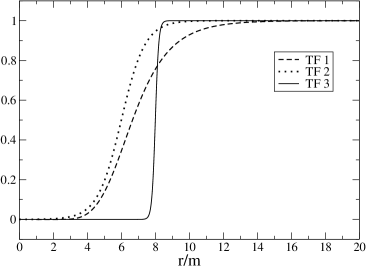
Figure 1: This figure shows the first (TF 1), second (TF 2) and third (TF 3) transition functions as a dashed, dotted and solid lines respectively. Observe that these functions transition at different radii and at different speeds.

Observe in figure 1 that the transition occurs at different radii and that they transition at different speeds. In  figure 2 we can observe the difference in the transitioning speed better. We can clearly see in this figure that the derivatives of TF 1 are the smallest, followed by TF 2 and then TF 3. However, both TF 1 and TF 2 have derivatives that are consistently of order much less than ${\cal{O}}(1)$, while TF 3 has first derivatives of ${\cal{O}}(1)$ or larger. The inset in this figure shows the large derivatives of TF 3. Also note that the second derivatives of the first and second transition functions are consistently smaller than their first derivatives. This is a consequence of the size of the transition window. If such a window were chosen to be smaller, as in the case of TF 3, then the second derivative would become larger than the first.

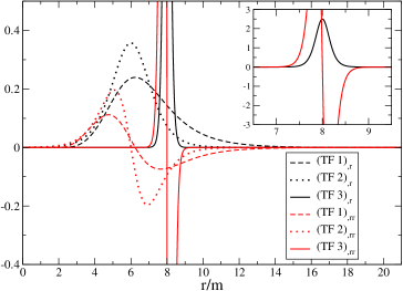
Figure 2: This figure shows the first and second derivatives of the transition functions. The first derivative of the first [$(TF~{}1)_{,r}$], second [$(TF~{}2)_{,r}$] and third [$(TF~{}3)_{,r}$] transition functions are denoted with a dashed, dotted and solid black line respectively. The second derivative of the first [$(TF~{}1)_{,rr}$], second [$(TF~{}2)_{,rr}$] and third [$(TF~{}3)_{,rr}$] transition functions are denoted with a dashed, dotted and solid cyan (or light gray on black and white print) line respectively. In the inset we zoomed out to show better the derivatives of the third transition function.

With these transition functions we can now construct pure joined solutions via

$$g_{\mu\nu}=f(\bar{r}_{1})f(\bar{r}_{2})g_{\mu\nu}^{(3)}+\left[1-f(\bar{r}_{1})\right]g_{\mu\nu}^{(1)}+\left[1-f(\bar{r}_{2})\right]g_{\mu\nu}^{(2)},$$ (53)

where we assume $g_{\mu\nu}^{(1,2)}$ has been transformed with the coordinate and parameter transformation of (4) and where $f(\cdot)$ can be any of TF 1, TF 2 or TF 3. Equation (53) is an extension of (11) applicable to two buffer zones. Extensions to more than $2$ buffer zones are also straightforward.

Whether the joined metric of (53) satisfies the Einstein equations to the same order as the approximate solution depends on the transition function used. We expect the metric constructed with TF 1 to generate small violations because it is a proper transition function that clearly satisfies the differentiability conditions required in Theorems 1 and 2. On the other hand, TF 2 and 3 do not satisfy these conditions because TF 2 is not a proper transition function and TF 3 violates condition $(ii)$ and $(iii)$ of Theorem 1. This behaviour, however, is not clear by simply looking at metric components. In figure 3 we plot the determinant of the spatial metric along the $x$-axis, corresponding to the $x$ harmonic (near zone) coordinate, with $t=0$, $y=0$ and $z=0$. This axis is where joined metrics are glued together with different transition functions. This determinant gives a measure of the volume element on $\Sigma$ and, as one can see in the figure, the difference when different transition function are used is small. This behaviour is not unique to the $x$-axis, but is actually observed along the other axis as well. When this is the case, we only show the behaviour along the $x$-axis in order to avoid redundancy.

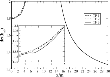
Figure 3: This figure shows the determinant of the spatial metric along the $x$-axis with TF 1 (dashed line), TF 2 (dotted line) and TF 3 (solid line.) Observe that the differences in the global metrics are small if at all visible. In the inset we zoom to the region where the curves look the most different.

Although the volume element computed with different transition functions is similar, metrics joined with different transition functions do not satisfy the Einstein equations to the same order. In  figure 4, we plot the $4$-Ricci scalar calculated with the global metrics joined with different transition functions. This plot is representative of the behaviour of the $4$-Ricci scalar in the entire domain, although here we plot it only along the $x$-axis. We also plot only the region $x/m>10$, to the right of where BH 1 is located at $t=0$, because the behaviour of the $4$-Ricci scalar is symmetric about $x=0$ and the transition functions are symmetric about $\bar{r}_{A}=0$. Thus, the behaviour of the $4$-Ricci scalar in other regions of the domain is similar to that shown in figure 4 (see paper I for contour plots of some of these quantities.)

There are several features in figure 4 that we should comment on. First, observe that the ${}^{(4)}R$ is everywhere smaller than the uncontrolled remainder in the approximate solutions (roughly ${\cal{O}}(m/b)^{2}\approx 0.0025$ in the buffer zone for the system considered) when the joined metric is constructed with TF 1. However, this is not the case for the metrics constructed with TF 2 and 3. For those metrics, ${}^{(4)}R$ has spikes close to $r_{A}=0$ ($x\approx 10m$) and $r_{A}=8m$ ($x\approx 18m$) for TF 2 and 3 respectively. The spike resulting from the metric constructed with TF 3 is associated with the small size of its transition window, which forces large derivatives in the transition function, thus violating conditions $(ii)$ and $(iii)$ of Theorems 1 and 2. The spike in the metric built with TF 2 is related to the fact that this function does not tend to zero faster than the uncontrolled remainders of the post-Newtonian near zone metric close to BH A. As we discussed earlier, the rate at which transition functions tend to zero and unity is important to avoid contamination from divergent uncontrolled remainders in the approximations. In this case, TF 2 is of ${\cal{O}}(m/b)^{3}$ as $r/m\to m/b$, while the post-Newtonian Ricci scalar diverges as $m/r^{3}$ as $r\to 0$ and is in fact of ${\cal{O}}(b/m)^{3}$ as $r/m\to m/b$. Since the transition function is not able to eliminate this contamination from the near zone metric, the Einstein equations are violated near either black hole for the metric constructed with TF 2. From a physical standpoint, the failure to use appropriate transition functions to create a pure joined solution introduces a modification in the matter-sector of the Einstein equations, namely the artificial creation of a shell of matter. One can straightforwardly see from (5) and (32) that the stress-energy tensor of this shell depends on the non-vanishing derivatives of the transition function.

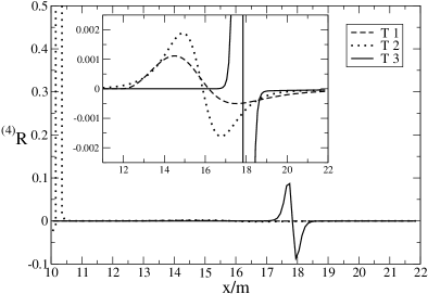
Figure 4: $4$-Ricci scalar along the x-axis for the global metrics joined with TF 1 (dashed line), TF 2 (dotted line) and TF 3 (solid line.) Observe that the $4$-Ricci scalar is small everywhere for the metric constructed with TF 1, but it has spikes for that built with TF 2 and 3. The inset zooms to the region $x\in[11,22]$ so that the difference between the $4$-Ricci scalar calculated with TF 1 and 2 are more noticeable.

A deeper analysis of the spike in ${}^{(4)}R$ due to the joined metric with TF 2 reveals that the conditions found are sufficient but formally not necessary. The $4$-Ricci scalar constructed with the post-Newtonian metric (${}^{(4)}R_{PN}$) diverges close to BH A, since this approximation breaks down in that region. Therefore, if the transition function does not vanish identically, or faster than the divergence in ${}^{(4)}R_{PN}$, then ${}^{(4)}R$ will present a spike. This spike, however, would disappear if the transition function decayed to zero faster than the divergence in ${}^{(4)}R_{PN}$. In this sense, eventhough the conditions discussed here are not necessary since the definition of a proper transition function could be weakened, they are certainly sufficient and universal.

The second feature we should comment on is the behaviour of ${}^{(4)}R$ in the region $x/m\in[11,17]$. As one can observe in the inset, the transition functions indeed introduce some error in this region. However, note that this error for the metric constructed with TF 1 is smaller than the uncontrolled remainders in the approximate solutions. Also note that this error is independent of the location of the center of the transition window. In other words, asymptotic matching is performed inside of a buffer zone and not on a patching surface, which means that approximate solutions can be glued with transition functions anywhere in the buffer zone away from the boundaries and not just at a specific $2$-surface. As one can see from the figure, the metric constructed with TF 1 has the smallest error in this region, followed by that built with TF 2 and 3. This fact is not too surprising because, as shown in the proof of Theorem 1, the error introduced by the transition functions in the calculation of the Ricci tensor scales with the first and second derivatives of these functions. Finally, note that the error introduced by these functions seems to be correlated to both the size and functional form of the second derivative of the transition functions, as one can see by comparing the inset of figure 2 to figure 4. The reason for such similarity, however, is beyond the scope of this paper.

Once an approximate global $4$-metric has been found, we can use it to construct initial data. These data could be given for example by

$$h_{ab} = f(\bar{r}_{1})f(\bar{r}_{2})h_{ab}^{(3)}+\left[1-f(\bar{r}_{1})\right]h_{ab}^{(1)}+\left[1-f(\bar{r}_{2})\right]h_{ab}^{(2)},$$

$$K_{ab} = f(\bar{r}_{1})f(\bar{r}_{2})K_{ab}^{(3)}+\left[1-f(\bar{r}_{1})\right]K_{ab}^{(1)}+\left[1-f(\bar{r}_{2})\right]K_{ab}^{(2)}.$$ (54)

Equation (4) is simply a generalization of (3.3) for $2$ buffer zones. The extrinsic curvatures for the inner zones and near zone are provided explicitly in paper I.

Are we allowed to construct data with transition functions in this way? There might be some doubt as to whether this is valid, since the fact that the joined metric satisfies the Einstein equations does not necessarily guarantee that we can use transition function to construct the data itself. In particular, there might be some worry that the extrinsic curvature calculated from (53) generally contains derivatives of the transition functions that (4) neglects. Theorem 2, however, ensures that this construction is indeed valid, provided the transition functions satisfy the same differentiability conditions proposed in Theorem 1. This is because the derivatives of these functions are then small and, in particular, the terms that are proportional to them are of the same order as the uncontrolled remainders in the approximations.

These expectations can be verified in figure 5, where we plot the $xy$-component of the extrinsic curvature along the $x$-axis constructed both via (4) (referred to as glued T 1, 2 and 3 in the figure) and by direct differentiation of (53) (referred to as full T 1, 2 and 3 in the figure.) We plot only the $xy$-component because this is the dominant term of this tensor along the $x$-axis for the system considered and it shows the main differences in using different transition functions. We have checked that other quantities, like the trace of the extrinsic curvature, behaves similarly. For contour plots of the extrinsic curvature refer to paper I.

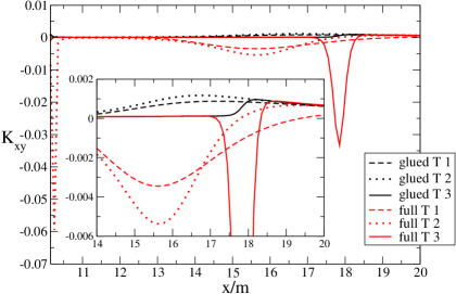
Figure 5: $xy$-component of the extrinsic curvature along the $x$-axis, constructed via (4) (black) for TF 1 (dashed line), TF 2 (dotted line) and TF 3 (solid line.) We also plot this component constructed by direct differentiation of (53) (cyan, or light gray on black and white print) for TF 1 (dashed line), TF 2 (dotted line) and TF 3 (solid line.) The inset zooms to the region $x\in\{15,22\}$ so that the differences are more noticeable.

As in the case of the Ricci scalar, there are several features of figure 5 that we should discuss. First, observe that that the extrinsic curvatures constructed with TF 1 agree in the buffer zone up to uncontrolled remainders. These remainders are of ${\cal{O}}(m/b)^{3/2}\approx 0.01$ in the buffer zone, because here we have used a coordinate transformation from the matching scheme that is valid only up to ${\cal{O}}(m/b)$. The inset zooms to a region close to the outer boundary of the buffer zone in order to show this agreement better. The humps in this region are produced by the non-vanishing Lie derivatives of the transition functions. Observe that, as expected, these humps are smallest for TF 1, followed by TF 2 and 3. Our analysis suggests that if we performed matching to higher order, the agreement would be better and the size of the humps would decrease. The agreement is good for the curvatures constructed with TF 1, but the curvatures built with TF 2 and 3 have strong spikes roughly near the boundary of the buffer zone. These spikes arise because TF 2 violates the definition of a proper transition function, while TF 3 violates conditions $(ii)$ and $(iii)$ of Theorem 2.

We have then seen in this section how Theorems 1 and 2 can aid us in constructing transition functions. Even though we have not shown the error in the constraints, we have checked that this error presents the same features as those shown in figure 4. We have also seen the importance of restricting the family of transition functions to those that satisfy conditions $(ii)$ and $(iii)$ of Theorems 1 and 2, as well as the definition of a proper transition function. The construction of pure, or mixed, joined solutions can then be carried out with ease as long as transitions functions are chosen that satisfy the conditions suggested here.

5 Conclusion

We studied the construction of joined solutions via transition functions. In particular, we focused on pure joined solutions, constructed by gluing analytical approximate solutions inside some buffer zone where they were both valid. The gluing process was accomplished via a weighted-linear combination of approximate solutions with certain transition functions. We constrained the family of allowed transition functions by imposing certain sufficient conditions that guarantee that the pure joined solution satisfies the Einstein equations to the same order as the approximations. With these conditions, we formulated and proved a theorem that ensures that the joined solution is indeed an approximate solution to the Einstein equations. We extended these conditions to projections of the joined solution onto a Cauchy hypersurface. We verified that the data on this hypersurface can itself be constructed as a weighted-linear combination with the same transition functions as those used for the joined solution. We proved that if these functions satisfy the same sufficient conditions, the data is guaranteed to solve the constraints of the Einstein equations to the same order as the approximations.

We explicitly verified these theorems numerically by considering a binary system of non-spinning black holes. The approximate solutions used were a post-Newtonian expansion in the far field and a perturbed Schwarzschild solution close to the black holes. We considered three different kinds of transition functions, two of which violated the conditions proposed in the theorems. The joined solutions constructed with these transition functions were shown to produce large violations to the Einstein equations. These violations were interpreted as the introduction of a matter-shell, whose stress-energy tensor was shown to be related to derivatives of the transition functions. The joined solution constructed with the transition function that did satisfy the conditions of the theorems was seen to introduce error comparable to that already contained in the approximate solutions. We further verified that projections of this joined solution to a Cauchy hypersurface can also be constructed as a weighted-linear combination of projections of approximate solutions with transition function. These joined projected solutions were seen to still satisfy the constraints of the theory to the same order as the approximate solutions provided the transition functions satisfied the conditions of the theorems.

The glue proposed here to join approximate solutions has several applications to different areas of relativistic gravitation. Initial data for numerical simulations could, for example, be constructed once approximate solutions to the system have been found and asymptotically matched inside some buffer zone. In particular, initial data for a binary system of spinning black holes could be generated by asymptotically matching and gluing a tidally perturbed Kerr metric [32] to a post-Newtonian expansion (see  [33].) One could also study the absorption of energy and angular momentum [34], as well as the motion of test particles [35], in the spacetime described by such pure joined solutions. Finally, one could extend the scheme developed here to formalize the construction of mixed joined solutions. Such solutions could, for example, be composed of a post-Newtonian metric glued to a numerically simulated metric or a semi-analytical approximate metric [10, 11, 36, 37]. Such mixed joined solutions could then be used to construct reliable waveform templates for extremely non-linear physical scenarios.

References

References

- [1] Alex Abramovici et al. Ligo: The laser interferometer gravitational wave observatory. Science, 256:325–333, 1992.
- [2] B. Willke et al. The geo 600 gravitational wave detector. Class. Quant. Grav., 19:1377–1387, 2002.
- [3] A. Giazotto. The virgo project: A wide band antenna for gravitational wave detection. Nucl. Instrum. Meth., A289:518–525, 1990.
- [4] M. Ando. Current status of tama. Class. Quant. Grav., 19:1409–1419, 2002.
- [5] K. Danzmann. Lisa - an esa cornerstone mission for a gravitational wave observatory. Class. Quant. Grav., 14:1399–1404, 1997.
- [6] Lisa. lisa.jpl.nasa.gov.
- [7] Luc Blanchet. Gravitational radiation from post-newtonian sources and inspiralling compact binaries. Living Rev. Rel., 5:3, 2002. and references therein.
- [8] Nicolas Yunes, Wolfgang Tichy, Benjamin J. Owen, and Bernd Brügmann. Binary black hole initial data from matched asymptotic expansions. Phys. Rev., D74:104011, 2006.
- [9] Nicolas Yunes and Wolfgang Tichy. Improved initial data for black hole binaries by asymptotic matching of post-newtonian and perturbed black hole solutions. Phys. Rev., D74:064013, 2006.
- [10] Alessandra Buonanno and Thibault Damour. Transition from inspiral to plunge in binary black hole coalescences. Phys. Rev., D62:064015, 2000.
- [11] Alessandra Buonanno, Yanbei Chen, and Thibault Damour. Transition from inspiral to plunge in precessing binaries of spinning black holes. Phys. Rev., D74:104005, 2006.
- [12] Carl M. Bender and Steven A. Orszag. Advanced mathematical methods for scientists and engineers 1, Asymptotic methods and perturbation theory. Springer, New York, 1999. and references therein.
- [13] J. Kevorkian and J. D. Cole. Multiple scale and singular perturbation methods. Springer, New York, 1991. and references therein.
- [14] W. L. Burke. J. Math. Phys., 12:401, 1971.
- [15] W. L. Burke and K. S. Thorne. Gravitational radiation damping. In M. Carmeli, S. I. Fickler, and L. Witten, editors, Relativity, pages 209–228. Plenum Press, 1970.
- [16] Peter D. D’Eath. Dynamics of a small black hole in a background universe. Phys. Rev., D11:1387, 1975.
- [17] Peter D. D’Eath. Interaction of two black holes in the slow-motion limit. Phys. Rev., D12:2183, 1975.
- [18] Kip S. Thorne and James B. Hartle. Laws of motion and precession for black holes and other bodies. Phys. Rev., D31:1815–1837, 1985.
- [19] Yasushi Mino, Misao Sasaki, and Takahiro Tanaka. Gravitational radiation reaction. Prog. Theor. Phys. Suppl., 128:373–406, 1997.
- [20] C. Lanczos. Bemerkung zur de sitterschen welt. Phys. Zeits., 23:539, 1922.
- [21] C. Lanczos. Fl’́achenhafte verteilung der materie in der einsteinschen gravitationsheorie. Ann der Phys., 74:528, 1924.
- [22] G. Darmois. Les équations de la gravitation einsteinienne. in Mémorial des sciences mathematíques XXV, Gauthier-Villars, Paris, 1927.
- [23] A. Lichnerowicz. Théories Relativistes de la Gravitation et de l’Electromagnétisme. Paris: Masson, 1955.
- [24] C. W. Misner and D. H. Sharp. Relativistic equations for adiabatic spherically symmetric gravitational collapse. Phys. Rev., B136:571, 1964.
- [25] C. Barrabes and W. Israel. Thin shells in general relativity and cosmology: The lightlike limit. Phys. Rev., D43:1129–1142, 1991.
- [26] W. Israel. Singular hypersurfaces and thin shells in gr. Nuovo Cimento, B44:1–14, 1966.
- [27] M. Misner, Charles, Kip S. Thorne, and John A. Wheeler. Gravitation. Freeman, New York, 1970. and references therein.
- [28] E. Poisson. A Relativist’s Toolkit: The mathematics of black-hole mechanics. Cambridge, New York, United States, 2004. and references therein.
- [29] Olivier Poujade and Luc Blanchet. Post-newtonian approximation for isolated systems calculated by matched asymptotic expansions. Phys. Rev., D65:124020, 2002.
- [30] Thomas W. Baumgarte and Stuart L. Shapiro. Numerical relativity and compact binaries. Phys. Rept., 376:41–131, 2003. and references therein.
- [31] Wolfgang Tichy, Bernd Brügmann, Manuela Campanelli, and Peter Diener. Binary black hole initial data for numerical general relativity based on post-newtonian data. Phys. Rev., D67:064008, 2003.
- [32] Nicolas Yunes and Jose A. Gonzalez. Metric of a tidally perturbed spinning black hole. Phys. Rev., D73:024010, 2006.
- [33] H. Tagoshi, A. Ohashi, and B. J. Owen. Gravitational field and equations of motion of spinning compact binaries to post-newtonian order. Phys. Rev., D 63:440006, 2001.
- [34] Eric Poisson. Absorption of mass and angular momentum by a black hole: Time-domain formalisms for gravitational perturbations, and the small-hole / slow-motion approximation. Phys. Rev., D70:084044, 2004.
- [35] Scott A. Hughes. Evolution of circular, non-equatorial orbits of kerr black holes due to gravitational-wave emission. ii: Inspiral trajectories and gravitational waveforms. Phys. Rev., D64:064004, 2001.
- [36] Carlos F. Sopuerta, Nicolas Yunes, and Pablo Laguna. Gravitational recoil from binary black hole mergers: The close-limit approximation. Phys. Rev., D74:124010, 2006.
- [37] Carlos F. Sopuerta, Nicolas Yunes, and Pablo Laguna. Gravitational recoil velocities from eccentric binary black hole mergers. Astrophys. J., 656:L9–L12, 2007.