A dynamical system approach to higher order gravity (Talk given at IRGAC 2006, July 2006)

Abstract

The dynamical system approach has recently acquired great importance in the investigation on higher order theories of gravity. In this talk I review the main results and I give brief comments on the perspectives for further developments.

1 Introduction

Since the very first proposal of General Relativity alternative formulations of the law of gravity have been proposed for various purposes: from unification of the fundamental interaction to the explanation of the dark energy phenomenon. In spite of the great variety of proposals, all these attempts present a common drawback: they are much more complicated than General Relativity. This means that it is very difficult to devise tests on these theories, and hence there are not many opportunities to gain insights on the their physics.

Obtaining such information is critical to the debate about the nature of gravitation and its relation with the dark energy issue. Particularly important in these respect are the indirect methods, i.e. methods that allows to solve indirectly the gravitational field equations or to obtain a qualitative idea of how these solutions behave.

One very interesting methods of this type is based on the application of the dynamical system approach to cosmology. This method has been developed for general relativity since the 70s, and it has lead to beautiful insights into the evolution of the anisotropic cosmologies [1].

In this paper we summarize the results obtained from the application of dynamical system theory to fourth order gravity and in particular to $R^{n}$-gravity. We also discuss very briefly some further applications of this method.

Unless otherwise specified, we will use natural units ($\hbar=c=k_{B}=8\pi G=1$) throughout the paper and Greek indices run from 0 to 3. The semicolon represents the usual covariant derivative and the “dot” corresponds to time differentiation.

2 $R^{n}-gravity$

The action for the gravitational interaction in this theory reads

$${\cal A}=\int d^{4}x\sqrt{-g}\left[\chi(n)R^{n}+{L}_{M}\right]\;,$$ (1)

where $\chi(n)$ is a positive function of $n$ that reduces to $1$ for $n=1$. For $R\neq 0$, the field equations for this theory can be written as

$$G_{\mu\nu}=T_{\mu\nu}^{M}+T_{\mu\nu}^{R}=\frac{\tilde{T}_{\mu\nu}^{M}}{n\chi(n)R^{n-1}}+\frac{1}{2n}g_{\mu\nu}(1-n)R+\left[(n-1)\frac{R^{;\alpha\beta}}{R}\right.$$

$$\left.+(n-1)(n-2)\frac{R^{;\alpha}R^{;\beta}}{R^{2}}\right](g_{\alpha\mu}g_{\beta\nu}-g_{\alpha\beta}g_{\mu\nu})\;,$$ (2)

where $\tilde{T}_{\mu\nu}^{M}$ is the stress energy tensor for the standard matter. In this way, the non-Einsteinian part of the gravitational interaction can be modelled as an effective fluid which, in general, presents thermodynamic properties different from standard matter . In the following we will analyze this equation in the Friedmann-Lemaître-Robertson-Walker (FLRW) and Bianchi I metrics with the aid of the dynamical system approach.

3 Dynamical analysis of the FLRW case

In the FLRW metric, the (2) take the form

$$2n\frac{\ddot{a}}{a}+n(n-1)H\frac{\dot{R}}{R}+n(n-1)\frac{\ddot{R}}{R}+n(n-1)(n-2)\frac{\dot{R}^{2}}{R^{2}}-(1-n)\frac{R}{3}$$

$$+\frac{\mu}{3n\chi(n)R^{n-1}}(1+3w)=0\;,$$ (3)

$$H^{2}+\frac{\kappa}{a^{2}}+H\frac{\dot{R}}{R}(n-1)-\frac{R}{6n}(1-n)-\frac{\mu}{3n\chi(n)R^{n-1}}=0\;.$$ (4)

$$\dot{\mu}+3H\mu(1+w)=0\;.$$ (5)

with

$$R=-6\left(\frac{\ddot{a}}{a}+\frac{\dot{a}^{2}}{a^{2}}+\frac{\kappa}{a^{2}}\right)$$ (6)

where $H=\dot{a}/a$, $\kappa$ is the spatial curvature index and we have assumed standard matter to be a perfect fluid with a barotropic index $w$. Note that in the above equations we have considered $a$ and $R$ as two independent fields so that the equation are of effective order two and the conservation equation for matter is the same as standard GR [2].

The form of the above equations suggests the following choice of expansion normalized variables:

$$x=\frac{\dot{R}}{RH}(n-1)\;,\ \ \ y=\frac{R}{6nH^{2}}(1-n)\;,\ \ \ z=\frac{\mu}{3n\chi(n)H^{2}R^{n-1}}\;,\ \ \ K=\frac{\kappa}{a^{2}H^{2}}\;,$$ (7)

Differentiating (7) with respect to the logarithmic time $\mathcal{N}=\ln a$, we obtain the autonomous system (matter is considered a perfect fluid)

$$x^{\prime}=\frac{2(n-2)y}{n-1}-2x-2x^{2}-\frac{xy}{n-1}+(1+x)z-3zw\;,$$

$$y^{\prime}=\frac{y}{n-1}\left[(3-2n)x-2y+2(n-1)z+2(n-1)\right]\;,$$ (8)

$$z^{\prime}=z\left(2z-1-3x-\frac{2y}{n-1}-3w\right)\;,1+x-y-z+K=0\;.$$

Note that the two planes $y=0$ and $z=0$ correspond to two invariant submanifolds. This implies that for this system no finite global attractor exists. The behavior of the scale factor corresponding the fixed points can be found using the equation

$$\dot{H}=\left(x_{C}+\frac{y_{C}}{n-1}-z_{C}-1\right)H^{2}\;.$$ (9)

If $n\neq 1$ and $(n-1)(x_{C}-z_{C}-1)-y_{C}\neq 0$ this equation can be integrated to give

$$a=a_{0}(t-t_{0})^{\alpha}\qquad\mbox{with}\qquad\alpha=\left(1-x_{C}-\frac{y_{C}}{n-1}+z_{C}\right)^{-1}\;.$$ (10)

In the same variables the energy density $\mu$ can be written as

$$\mu=zy^{n-1}H^{2n}\;,$$ (11)

thus for $n>1$ both the $(x,y)$ and $(x,z)$ planes are invariant vacuum manifolds, but if $n<1$ the vacuum submanifold is not necessarily compact.

A detailed analysis of this dynamical system is shown elsewhere [2]. Here we will focus on the interval $1.367\lesssim n<2$. This interval is suggested by a fitting of the data coming from WMAP and Supernovae Ia data [3].

3.0.1 The vacuum Case

In a vacuum spacetime (i.e. $\mu=0$), the variable $z$ is identically zero and the third equation of (3) becomes an identity. Let us analyze this case first. Setting $x^{\prime}=0$ and $y^{\prime}=0$, we obtain the four fixed points shown in Table 1.

Table 1: Coordinates of the finite and asymptotic fixed points and solutions for FLRW $R^{n}$-gravity in vacuum.

Point	Coordinates	Solution/Behaviour
$\mathcal{A}$	$[x,y]=[0,0]$	$a=a_{0}t$
$\mathcal{B}$	$[x,y]=[-1,0]$	$a=a_{0}(t-t_{0})^{1/2}$ (only for $n=3/2$)
$\mathcal{C}$	$[x,y]=\left[\frac{2(n-2)}{2n-1}\;,\frac{4n-5}{2n-1}\right]$	$a=a_{0}\;t^{\frac{(1-n)(2n-1)}{n-2}}$
$\mathcal{D}$	$[x,y]=\left[2(1-n)\;,2(n-1)^{2}\right]$	$a=a_{0}t$
$\left(\mathcal{A}_{\infty},\;\mathcal{C}_{\infty},\;\mathcal{D}_{\infty},\;\mathcal{F}_{\infty}\right)$	$\theta=\left(0,\;\pi/2,\;\pi,\;3\pi/2\right)$	$|{\cal{N}}-{\cal N}_{\infty}|=\left[C_{1}\pm\frac{C_{0}}{2}(t-t_{0})\right]^{2}$
$\left(\mathcal{B}_{\infty},\;\mathcal{E}_{\infty}\right)$	$\theta=\left(\pi/4,\;5\pi/4\right)$	$|{\cal N}-{\cal N}_{\infty}|=\left[C_{1}\pm C_{0}\left|\frac{n-1}{2n-1}\right|(t-t_{0})\right]^{\frac{2n-1}{n-1}}$

In our interval the solution associate with the point $\mathcal{C}$ is a power law inflation and the only finite attractor. This is an interesting result because this model contains cosmic histories that naturally approach to a phase of accelerate expansion. However, the presence of the invariant submanifolds already mentioned makes this attractor not global and we have to check if there are other attractors in asymptotic regime.

The idea that the system above might have a nontrivial asymptotic structure comes from the fact that the phase plane is not compact. The asymptotic analysis can be easily performed using the Poincaré approach [4]. We obtained six fixed points which are summarized with their behavior in Table 1. The stability analysis shows that in the interval of $n$ we have chosen there is another attractor (this time global): the point $\mathcal{D}_{\infty}$. Using the asymptotic limit of Equation 9 (see [2]), we found that $\mathcal{D}_{\infty}$ is associated with a Lemaître type evolution in which the universe reaches a maximum size and then recollapses. The presence of $\mathcal{D}_{\infty}$ reduces the measure of the set of initial conditions for which an orbit will approach to $\mathcal{C}$, or in simpler words it makes this type of cosmic histories “less probable”. A pictorial representation of the whole (compactified) phase space is given in Figure 1.

3.0.2 The non-vacuum Case

When matter is present we consider the full system (3). Setting $x^{\prime}=0$, $y^{\prime}=0$, $z^{\prime}=0$ and solving for $x,y,z$ we obtain seven fixed points and two fixed subspaces. The first four points lay on the plane $z=0$ and correspond to the vacuum fixed points. Of the other three fixed points, $\mathcal{G}$ is definitely the most interesting because of its associated solution: $\displaystyle{a=a_{0}t^{\frac{2n}{3(1+w)}},\;\;\mu=\mu_{0}t^{-2n}}$. The presence of such a fixed point brings the idea that there could be cosmic histories in this model in which a(n unstable) Friedmann-like phase is followed naturally by a phase of accelerated expansion. Applying the standard tools of the dynamical system, we discover that this is actually the case in our interval for $n$. In fact, for $1.367\lesssim n<2$ the point $\mathcal{C}$ is an attractor and the point $\mathcal{G}$ is a saddle, they are both physical and placed in a connected sector of the phase space. Thus in principle a cosmic history like the one pictured above is possible. This is also confirmed by numerical investigation of the dynamical system. The last thing to check is the presence of other attractors in the asymptotic regimes. The compactification is achieved in the same way as the vacuum case, but the equations obtained are much more complicated. Here we will limit ourselves to say that there are other attractors in the phase space, in the form of subspaces and single points and their presence reduce the measure of the set of initial conditions that lead to a cosmic history connecting $\mathcal{G}$ and $\mathcal{C}$.

4 Dynamical analysis of the LRS Bianchi I cosmologies

In order to obtain the simplest possible form for the field equations in the LRS Bianchi I metric, we use the 1+3 covariant approach to cosmology [5]. In this formalism the cosmological equations can be written as

$$\dot{\Theta}+{\textstyle{1\over 3}}\,\Theta^{2}+2\sigma^{2}-\frac{1}{2n}R-(n-1)\frac{\dot{R}}{R}\Theta+\frac{\mu}{\chi nR^{n-1}}=0,$$ (12)

$${\textstyle{1\over 3}}\,\Theta^{2}-\sigma^{2}+(n-1)\frac{\dot{R}}{R}\Theta-\frac{(n-1)}{2n}R-\frac{\mu}{\chi nR^{n-1}}=0\;,$$ (13)

$$\dot{\sigma}=-\left(\Theta+(n-1)\frac{\dot{R}}{R}\right)\sigma\;,$$ (14)

together with the (5). Here $\Theta$ is the volume expansion $\Theta=3{\textstyle{\dot{a}\over a}}=3H$ and $\sigma$ is the square root of the magnitude the symmetric shear tensor $\sigma_{ab}$. The set of expansion normalized variables is:

$$x=\frac{3\dot{R}}{R\Theta}(n-1)\;,\ \ \ \ y=\frac{3R}{2n\Theta^{2}}(n-1)\;,\ \ \ \ z=\frac{3\mu}{\chi nR^{n-1}\Theta^{2}}\;,\ \ \ \Sigma=\frac{3\sigma^{2}}{\Theta^{2}}\;,$$ (15)

and the dynamical system can be written as

$$\Sigma^{\prime}=-2\left[\left(\frac{2n-1}{n-1}\right)\;y+z\right]\Sigma,$$

$$y^{\prime}=\frac{y}{n-1}\left[(2n-1)\Sigma-(2n-1)y+z+(4n-5)\right],$$ (16)

$$z^{\prime}=z\left[(2-3w)-z+\Sigma-\left(\frac{3n-1}{n-1}\right)\;y\right],$$

$$1-\Sigma+x-y-z=0.$$

The solution associated to every fixed point can be found via the equations

$$\dot{\Theta}=\left(\frac{n}{n-1}y_{i}-\Sigma_{i}-2\right)\frac{\Theta^{2}}{3}\;,\qquad\qquad\dot{\sigma}=-\frac{1}{3}(2+\Sigma_{i}+y_{i}+z_{i})\;\Theta\;\sigma.$$ (17)

For $n\neq 1$, $\sigma\neq 0$ and a R.H.S. different from zero, these equations admit the solution

$$a=a_{0}\left(t-t_{0}\right)^{\alpha}, \qquad\alpha=\left(2+\Sigma_{i}-{\textstyle{n\over n-1}}y_{i}\right)^{-1}\;,$$ (18)

$$\sigma=\sigma_{0}a^{\beta}, \qquad\beta=-(2+\Sigma_{i}+y_{i}+z_{i})\;.$$ (19)

As in the previous section we will focus on a specific intervals of $n$ referring the reader to [6] for a general analysis.

4.0.1 The vacuum Case

In order to treat the vacuum case, we set $z=0$ and we neglect the equation for $z$ as in the FLRW case. Setting $\Sigma^{\prime}=0$ and $y^{\prime}=0$ we obtain the fixed subspaces and their solutions (see Table 2).

Table 2: The finite an asymptotic fixed points and eigenvalues for $R^{n}$-gravity in a LRS Bianchi I model.

Fixed subspaces	Coordinates	Scale Factor	Shear
$\tilde{\mathcal{A}}$	$(\Sigma,y)$=$\left(0,{\textstyle{4n-5\over 2n-1}}\right)$	$a=a_{0}\left(t-t_{0}\right)^{{\textstyle{(1-n)(2n-1)\over(n-2)}}}$	$\sigma=0$
$\mathcal{L}_{1}$	$(\Sigma,y)$=$\left(\Sigma_{*},0\right)$	$a=a_{0}\left(t-t_{0}\right)^{{\textstyle{1\over 2+\Sigma_{*}}}}$,	$\sigma=\sigma_{0}a^{-(2+\Sigma_{*})}$
$\mathcal{A}_{\infty}$	$\phi$=$0$	$\tau-\tau_{\infty}=\frac{1}{\Sigma_{c}}\ln\left|t-t_{0}\right|+C$	$\sigma=\sigma_{0}a^{-(2+\Sigma_{c})}$
$\left(\mathcal{B}_{\infty},\;\mathcal{C}_{\infty}\right)$	$\phi$=$\left(\frac{\pi}{2}\;,\frac{3\pi}{2}\right)$	$|\tau-\tau_{\infty}|=\left[C_{1}\pm C_{0}\left|{\textstyle{n-1\over 2n-1}}\right|(t-t_{0})\right]^{\frac{2n-1}{n-1}}$	$\sigma=0$
$\mathcal{D}_{\infty}$	$\phi$=${\textstyle{7\pi\over 4}}$	$|\tau-\tau_{\infty}|=\left[C_{1}\pm C_{2}(t-t_{0})\right]^{2}$	$\sigma=\sigma_{0}$

Note that the fixed point $\tilde{\mathcal{A}}$ represents the same solution associated to the point $\mathcal{A}$. Direct verification with the cosmological equations reveals that this point is anisotropic i.e. $\sigma_{ab}=0$. The presence of such a point is particularly interesting because it means that there could be cosmic histories in which there is an isotropic state for an otherwise anisotropic universe. Two interesting cases arise. When $1<n<5/4$, the point $\tilde{\mathcal{A}}$ is a repeller and part of the orbits emerging from it approach the fixed line. This means that in these cosmic histories the universe starts in an isotropic state and then develops anisotropies (see figure 1). The presence of an isotropic past attractor is not present in GR and implies that in $R^{n}$-gravity, like in brane cosmology, there is no need for special initial conditions for inflation to begin [6]. When $n>5/4$, $\tilde{\mathcal{A}}$ is an (isotropic) attractor and all the orbits above the fixed line start on $\mathcal{L}_{1}$ and converge to it (see Figure 1). This scenario presents the same smooth transition between a decelerated and accelerated expansion of the FLRW case.

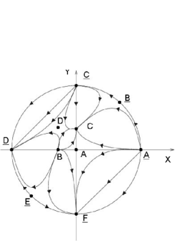
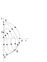
Figure 1: Global (compactified) phase spaces for $R^{n}$-gravity. The first picture represent the FLRW case with $1.36\lesssim n<2$; the second the Bianchi I case for $1<n<5/4$ and the third the Bianchi I $n>5/4$ case. The standard capital letters represent the finite fixed points the underlined capital letters represent the asymptotic fixed points. The point $\Sigma$ is nor a fixed point but it is defined as the last attractive point of the fixed line. The curly capital “l” represents the line $\mathcal{L}_{1}$.

If we analyze the asymptotic regime for this last case we can see that for $n>5/4$ the point $\mathcal{D}_{\infty}$ is an attractor (see Table 2), but is in a separate section of the phase space with respect to $\tilde{\mathcal{A}}$, sot that $\tilde{\mathcal{A}}$ can be considered an “effective” global attractor.

4.0.2 The Matter Case

Setting $\Sigma^{\prime}=0$, $y^{\prime}=0$ and $z^{\prime}=0$ in (4) we obtain, together with the vacuum fixed points, other two fixed points, one of which ($\tilde{\mathcal{G}}$) is an isotropic point associated with the same solution of $\mathcal{G}$. Let us check if it is possible to have a cosmic history similar to the one we found in FLRW. For $n>5/4$, the fixed line contains repulsive points nearby the origin, the point $\tilde{\mathcal{G}}$ is unstable and the point $\tilde{\mathcal{A}}$ in an attractor. Since these points are not separated by any invariant subspace, there is in principle an orbit that connects them. Along this orbit, the universe would start in an anisotropic state, evolve towards a more isotropic state to smoothly approach to a phase of accelerated expansion. Of course the issue of determining how many other attractors are present (and so how “probable” this evolution is) is still present and we have to perform a detailed asymptotic analysis in order to understand this point. Using the results of [6] it is possible to show that there are other attractors in the phase space that might influence the global evolution. However, the outcome is that an orbit like the one described above is still possible and surely deserves more study.

5 Conclusion

In this paper we hope to have shown how useful and powerful the dynamical system approach is in dealing with complicated model like fourth order gravity ones. The application of this method has allowed new insights on higher order cosmological models and has shown a deep connection between these theories and the cosmic acceleration phenomenon, which is worth to be further studied.

The perspective for future application of the dynamical system approach to higher order gravity can be basically divided in two thrusts. The first one is to analyze more complicated Lagrangians. Some of work in this direction has already started in [7] with quadratic gravity. The second one is the generalization to more complicated metrics, which will allow us to consider different physical framework. In the future, both of these thrusts will make possible not only to develop experimental test for alternative gravity but also to allow a better understanding of the reasons underlying the success of General Relativity.

References

References

- [1] Dynamical System in Cosmology edited by Wainwright J and Ellis G F R (Cambridge: Cambridge Univ. Press 1997) and references therein
- [2] S. Carloni, P. K. S. Dunsby, S. Capozziello and A. Troisi, Class. Quant. Grav. 22 (2005) 4839 and references therein [arXiv:gr-qc/0410046]
- [3] S. Capozziello, V. F. Cardone, S. Carloni and A. Troisi, Int. J. Mod. Phys. D 12 (2003) 1969 [arXiv:astro-ph/0307018]
- [4] see for example S. Lefschetz, Differential Equations: Geometric Theory Dover, New York (1977)
- [5] G. F. R. Ellis and H. van Elst, arXiv:gr-qc/9812046
- [6] J. A. Leach, S. Carloni and P. K. S. Dunsby, Class. Quant. Grav. 23 (2006) 4915 and references therein [arXiv:gr-qc/0603012].
- [7] J. D. Barrow and S. Hervik, arXiv:gr-qc/0610013