Gauge invariant perturbations of Scalar-Tensor Cosmologies I: The vacuum case

Abstract

The covariant gauge invariant perturbation theory of scalar cosmological perturbations is developed for a general Scalar-Tensor Friedmann-Lemaitre-Robertson-Walker cosmology in a vacuum. The perturbation equations are then solved exactly in the long wavelength limit for a specific coupling, potential and background. Differences with the minimally coupled case are briefly discussed.

I Introduction

In the last few years a tremendous advance in the accuracy of cosmological observations has revolutionised our understanding of the dynamics of the Universe. In particular, it has been realized that the universe is evolving in a way that is incompatible with what one would expect in a homogeneous and isotropic baryon dominated universe. One way of dealing with this problem is to suppose that the Universe is still homogeneous and isotropic but dominated by a different form of energy density: the so called Dark Energy (DE). Many different ideas regarding the nature of DE have been proposed in the last few years, ranging from the cosmological constant bi:cosmconst to Quintessence bi:quintessence , Chaplygin gas bi:chaplygin and Phantom energy bi:phantom , but so far none of them has provided a fully satisfactory solution to the problem.

Another interesting approach is based on the hypothesis that on cosmological scales gravity works in a slightly different way than in General Relativity (GR). In this way DE acquires a geometrical character, i.e. some of the observations can be explained by having a different behaviour of gravity on cosmological scales, rather than a new (and as yet undiscovered) form of energy density.

The idea that gravity might work differently on different scales is suggested by many fundamental schemes such as quantum field theory in curved spacetime bi:donoghue , as well as the compactification of internal spaces in multidimensional gravity Les82 ; fuji maeda , the low energy limit of string theory Mtheory and some braneworld models bi:chiba . Furthermore, GR has only been well tested on small scales and at low energies, so currently we lack strong constraints in the other regimes. In this respect cosmology is an ideal testing ground because it offers an indirect way to test GR on scales and at energies which are not achievable in Earth-bound laboratories, but were realized throughout the history of the universe. Therefore, investigations of cosmology in alternative theories of GR has a double relevance; it contributes to the understanding of DE and provides a testing ground for GR on different scales.

A key step in investigating the cosmology of an alternative theory of gravity is the development of a full theory of cosmological perturbations. This will make it possible to use some of the best and most precise sets of observational data currently available, such as the WMAP observations of the Cosmic Microwave Background (CMB) anisotropies, allowing us to understand the viability of these theories and constrain their parameters.

In this paper, we will develop the theory of linear scalar perturbations for one of the most studied extensions of GR: Scalar-Tensor theories of gravity. This will be done using the 1+3 covariant and gauge invariant approach, developed in bi:ellis2 and successfully applied to GR in the presence of minimally coupled scalars field bi:peterscalar . Although this formalism can be applied to perturbations of any spacetime, our work will be focused only on almost Friedmann-Lemaitre-Robertson-Walker (FLRW) universes which correspond to standard linear perturbations of FLRW models (see bi:EBH for details) and in absence of standard matter. The non-vacuum case will be treated in a forthcoming paper. Scalar field dominated universes in the Scalar-Tensor framework have attained prominence through the Extended and Hyper-extended Inflation scenarios bi:inflext ; bi:inflhyperext , so an analysis of the evolution of perturbations is important for obtaining a complete description of structure-formation in these models. In addition, the general formalism presented here could be used in situations different from inflation in which a scalar field dominates. As in bi:peterscalar , emphasis is given here to curvature perturbations bi:hawking , which are naturally gauge invariant, rather than metric perturbations bi:bardeen ; bi:ks ; bi:brand which play no explicit role. Bardeen’s formalism has been applied to this situation in specific cases of coupling, potential and background bi:salv1 . There has also been quite an extensive analysis of perturbations in non-standard theories of gravity given by Hwang in bi:hwangall . The aim of this paper is to give the general perturbation equations for a general coupling, potential and (FLRW) background using the full covariant approach to cosmologyand choosing  a set of variables which are as much as possible of straightforward physical interpretation.

The paper is organised as follows. In section II, after a few preliminary remarks on Scalar-Tensor gravity, we set up the formalism based on the natural slicing of the problem $\{\phi=const\}$ and on its geometric characterisation through the unit vector $u^{a}$, which is orthogonal to these surfaces. We also characterise the effective thermodynamics of the non-minimally coupled field by treating it as an effective fluid. In section III we specify the general features of the background and define the key gauge invariant dimensionless variables. In section IV we present the general perturbation equations, and, after specifying the coupling, the potential and the background, we give an exact solution of the perturbation equations in the large wavelength limit. In section 5, we work out a specific example giving an exact solution in the long wavelength limit i.e. on super-horizon scales.

Unless otherwise specified, natural units ($\hbar=c=k_{B}=8\pi G=1$) will be used throughout this paper, Latin indices run from 0 to 3. The symbol $\nabla$ represents the usual covariant derivative and $\partial$ corresponds to partial differentiation. We use the $-,+,+,+$ signature and the Riemann tensor is defined by

$$R^{a}{}_{bcd}=W_{bd,c}^{a}-W_{bc,d}^{a}+W_{bd}^{e}W_{ce}^{a}-W_{bc}^{f}W_{df}^{a}\;,$$ (1)

where the $W_{bd}^{a}$ is the Christoffel symbol (i.e. symmetric in the lower indices), defined by

$$W_{bd}{}^{a}=\frac{1}{2}g^{ae}\left(g_{be,d}+g_{ed,b}-g_{bd,e}\right)\;.$$ (2)

The Ricci tensor is obtained by contracting the first and the third indices

$$R_{ab}=g^{cd}R_{acbd}\;.$$ (3)

Finally the Hilbert–Einstein action in presence of matter is defined by

$${\cal A}=\int dx^{4}\sqrt{-g}\left[\frac{1}{2}R+L_{m}\right]\;.$$ (4)

II Preliminaries

II.1 Scalar Tensor Theories of Gravity

Scalar-Tensor theories of gravity involve a new degree of freedom of the gravitational interaction in a form of a scalar field non-minimally coupled to the geometry. These theories were first proposed as a modification of GR able to completely include Mach’s principle bi:BransDicke . From a technical standpoint, this can be achieved by allowing the Gravitational constant $G$ to vary throughout the spacetime, and in particular to be a function of a scalar field (so that frame effects are avoided). However, such a scalar cannot be found within GR because they can contain first derivatives of the metric and fall off more rapidly than $r^{-1}$. As a consequence, $G$ is imagined to depend on an additional scalar field $\phi$.

Like many of the extensions of GR, scalar-tensor theories appear in many fundamental schemes and have been proposed as models for dark energy because their cosmology naturally leads to the phenomenon of cosmic acceleration, which is the characteristic footprint of dark energy ScTnDarkEnergy ; Claudio .

The most general action for Scalar Tensor Theories of gravity is given by (conventions as in Wald bi:wald )

$$\mathcal{A}=\int dx^{4}\sqrt{-g}\left[\frac{1}{2}F(\phi)R-\frac{1}{2}\nabla_{a}\phi\nabla^{a}\phi-V(\phi)+\mathcal{L}_{m}\right]\;,$$ (5)

where $V(\phi)$ is a general (effective) potential expressing the self interaction of the scalar field and $\mathcal{L}_{m}$ represents the matter contribution.

Varying the action with respect to the metric gives the gravitational field equations:

$$F(\phi)G_{ab}=F(\phi)\left(R_{ab}-\frac{1}{2}\,g_{ab}R\right)=$$

$$=T_{ab}^{m}+\nabla_{a}\phi\nabla_{b}\phi-g_{ab}\left(\frac{1}{2}\nabla_{c}\phi\nabla^{c}\phi+V(\phi)\right)+\left(\nabla_{b}\nabla_{a}-g_{ab}\nabla_{c}\nabla^{c}\right)F(\phi)\;,$$ (6)

while the variation with respect to the field $\phi$ gives the curved spacetime version of the Klein - Gordon equation

$$\nabla_{a}\nabla^{a}\phi+\frac{1}{2}F^{\prime}(\phi)R-V^{\prime}(\phi)=0\;,$$ (7)

where the prime indicates a derivative with respect to $\phi$. Both these equations reduce to the standard equations for GR and a minimally coupled scalar field when $F(\phi)=1$.

Equation (6) can be recast as

$$G_{ab}=\frac{T_{ab}^{m}}{F(\phi)}+T^{\phi}_{ab}=T^{(eff)}_{ab}\,,$$ (8)

where $T^{\phi}_{ab}$ has the form

$$T_{ab}^{\phi}=\frac{1}{F(\phi)}\left[\nabla_{a}\phi\nabla_{b}\phi-g_{ab}\left(\frac{1}{2}\nabla_{c}\phi\nabla^{c}\phi+V(\phi)\right)+\nabla_{b}\nabla_{a}F(\phi)-g_{ab}\nabla_{c}\nabla^{c}F(\phi)\right]\;.$$ (9)

Provided that $\phi_{,a}\neq 0$, equation (7) also follows from the conservation equations

$$\nabla^{b}T_{ab}^{\phi}=0\;.$$ (10)

The fact that the gravitational field equation can be written in this form is crucial for our purposes. In fact, the form of (8) allows us to treat scalar tensor gravity as standard Einstein gravity in presence of two effective fluids with energy momentum tensor $\frac{2T_{ab}^{m}}{F(\phi)}$ and $T^{\phi}_{ab}$. This implies that, once the effective thermodynamics of these fluids has been studied, we can apply the standard covariant and gauge-invariant approach to cosmology. In this paper we will consider only the vacuum $T_{ab}^{m}=0$ case, leaving the non-vacuum case to a future paper.

II.2 Kinematical quantities

In order to give a proper description of the kinematics of the effective fluid associated with the scalar field we have to assign a 4-velocity vector $u^{a}$ to the scalar field itself. Following bi:peterscalar ; bi:madsen we assume that the momentum density $\nabla^{a}\phi$ is timelike:

$$\nabla_{a}\phi\nabla^{a}\phi<0\;,$$ (11)

in the open region $A$ of spacetime we are dealing with. This has two important consequences: Firstly ${\mathit{\phi}=const.}$ specifies well-defined surfaces in spacetime and secondly, these surfaces are spacelike (as consequence of (11)). We can therefore choose the 4-velocity $u^{a}$ to be the normalised timelike vector

$$u^{a}\equiv-\frac{\nabla^{a}\phi}{\psi}\;,~{}~{}~{}u^{a}u_{a}=-1\;,~{}~{}~{}\psi\equiv\dot{\phi}=u^{a}\nabla_{a}\phi=(-\nabla_{a}\phi\nabla^{a}\phi)^{1/2}\;,$$ (12)

where $\psi=\dot{\phi}$ denotes the magnitude of the momentum density (simply momentum from now on). The vector (12) is timelike because it is parallel to the normals of (i.e. orthogonal to) the surfaces $\{\phi=const.\}$ and it is also unique because, since these surfaces are well defined, their normals are unique.

Note that this definition might not appear well posed in general because $\phi$ could oscillate and change sign even in an expanding universe. However, equation (11) and the regularity of the behaviour of $\phi$ (see bi:peterscalar for more details) ensures the possibility of an extension by continuity.

Once the velocity field has been chosen, the projection tensor into the tangent 3-spaces orthogonal to the flow vector can be defined as:

$$h_{ab}\equiv g_{ab}+u_{a}u_{b}\;\Rightarrow h^{a}{}_{b}h^{b}{}_{c}=h^{a}{}_{c}\;,~{}h_{ab}u^{b}=0\;,$$ (13)

and the derivation of the kinematical quantities can be obtained by splitting the covariant derivative of $u_{a}$ into its irreducible parts bi:ellis2 :

$$\nabla_{b}u_{a}=\tilde{\nabla}_{b}u_{a}-A_{a}u_{b}\;,~{}~{}~{}\tilde{\nabla}_{b}u_{a}=\frac{1}{3}\Theta h_{ab}+\sigma_{ab}+\omega_{ab}\;,$$ (14)

where $\tilde{\nabla}_{a}$ is the totally projected covariant derivative operator orthogonal to $u^{a}$, $A_{a}=\dot{u}_{a}$ is the acceleration ($A_{b}u^{b}=0$), $\Theta$ is the expansion parameter, $\sigma_{ab}$ the shear ($\sigma^{a}{}_{a}=\sigma_{ab}u^{b}=0$) and $\omega_{ab}$ is the vorticity ($\omega_{ab}=\omega_{[ab]}$, $\omega_{ab}u^{b}=0)$.

Important consequences of the choice (12) are

$$\tilde{\nabla}_{a}\phi=0,$$ (15)

i.e. the surfaces $\{\phi=const.\}$ are the 3-spaces orthogonal to $u^{a}$, and

$$\Theta = -\tilde{\nabla}_{a}(\frac{\nabla^{a}\phi}{\psi})=-\frac{1}{\psi}\left[F^{\prime}(\phi)R-V^{\prime}(\phi)+\dot{\psi}\right]\neq 0\;,$$ (16)

$$\sigma_{ab} = -\frac{1}{\psi}\,h_{a}{}^{c}h_{b}{}^{d}\nabla_{(c}\left[\nabla_{d)}\phi\right]+\frac{1}{3}h_{ab}\nabla_{c}(\frac{\nabla^{c}\phi}{\psi})\neq 0\;,$$ (17)

$$A_{a} = -\frac{1}{\psi}\,\tilde{\nabla}_{a}\psi=-\frac{1}{\psi}(\nabla_{a}\psi+u_{a}\dot{\psi})\neq 0\;,$$ (18)

where the last equality in (16) follows on using the Klein - Gordon equation (7). We can see from (18) that $\psi$ is an acceleration potential for the fluid flow bi:ellis2 . Note also that, as consequence of (15), the vorticity vanishes:

$$\omega_{ab}=-h_{a}{}^{c}h_{b}{}^{d}\nabla_{[d}\left(\frac{1}{\psi}\nabla_{c]}\phi\right)=0\;,$$ (19)

which implies that $\tilde{\nabla}_{a}$ is the actual covariant derivative operator in the 3-spaces ${\mathit{\phi}=const}$ . Finally, it is useful to introduce a scale length $a$ along each flow - line so that

$$\frac{\dot{a}}{a}\equiv\frac{1}{3}\Theta=H\;,$$ (20)

where $H$ is the usual Hubble parameter if the Universe is homogeneous and isotropic.

II.3 The non-minimally coupled scalar field as an effective imperfect fluid

Using the definition of the 4-velocity given above, we can deduce the thermodynamical properties of the effective fluid described by the non minimally coupled scalar field. The general form of the energy momentum tensor (9) is:

$$T_{ab}^{\phi}=\mu_{\phi}u_{a}u_{b}+p_{\phi}h_{ab}+q_{a}^{\phi}u_{b}+q_{b}^{\phi}u_{a}+\pi_{ab}^{\phi}\;,$$ (21)

where the energy density $\mu_{\phi}$ and pressure $p_{\phi}$ of the scalar field “fluid” are:

$$\mu_{\phi}=\frac{1}{F(\phi)}\left[\frac{1}{2}\psi^{2}+V(\phi)-\Theta\dot{F}(\phi)\right]\;,$$ (22)

$$p_{\phi}=\frac{1}{F(\phi)}\left[\frac{1}{2}\psi^{2}-V(\phi)+\left(\ddot{F}(\phi)+\frac{2}{3}\Theta\dot{F}(\phi)\right)\right]\;,$$ (23)

and the energy flux and anisotropic pressure are given by:

$$q_{a}^{\phi}=\frac{\dot{F}(\phi)}{F(\phi)}\;A_{a}\;,$$ (24)

$$\pi_{ab}^{\phi}=-\frac{\dot{F}(\phi)}{F(\phi)}\;\sigma_{ab}\;.$$ (25)

Since the anisotropic pressure $\pi_{ab}$ and the heat flux $q_{a}$ are different from zero, the effective fluid associated with a non-minimally coupled scalar field is, in general, imperfect. The form of (24) and (23) shows explicitly that this is a direct consequence of the non-minimal coupling and that, when $\phi$ is minimally coupled (i.e. $F(\phi)=1=constant$) we have $q_{a}=0=\pi_{ab}$. This is in agreement with the results of bi:peterscalar , in which a minimally coupled scalar field is considered to be a perfect fluid. It is also worth noting that, since $\pi_{ab}$ and $q_{a}$ depend on the acceleration and the shear, when we consider FLRW universes, where these quantities vanish, the effective fluid behaves like a perfect fluid . However this is not true in the perturbed universe.

The twice contracted Bianchi Identities lead to the energy and momentum conservation equations:

$$\dot{\mu}+\Theta(\mu+p)+\pi_{ab}\sigma^{ab}+\tilde{\nabla}_{a}q^{a}+a_{a}q^{a}=0\;,$$ (26)

and

$$A_{a}(\mu+p)+\tilde{\nabla}_{a}p+h^{c}{}_{a}\left(\tilde{\nabla}_{b}\pi^{b}{}_{c}+\dot{q}_{c}\right)+\left(\sigma^{b}{}_{a}+\frac{4}{3}\Theta h^{b}{}_{a}\right)q_{b}=0\;.$$ (27)

If we now substitute $\mu$ and $p$ from (22) and (23) into (26), we obtain, as expected, the Klein - Gordon equation (7):

$$\ddot{\phi}+\Theta\dot{\phi}-\frac{1}{2}F^{\prime}(\phi)R+V^{\prime}(\phi)=0\;,$$ (28)

an exact ordinary differential equation for $\phi$ in any space - time with the choice (12) for the four - velocity. With the same substitution, (27) becomes an identity for the acceleration potential $\psi$.

In our calculation the ratio between the pressure $p$ and energy density $\mu$ of the effective fluid defined above is given by

$$w=-1+\frac{1}{\mu F(\phi)}\left[\psi^{2}+\frac{1}{3}\Theta\dot{F}(\phi)+\ddot{F}(\phi)\right]\;.$$ (29)

This is a useful parameter of the theory, but should not be confused with the barotropic factor typical of perfect fluids. In the same way, the quantity $\frac{\dot{p}}{\dot{\mu}}$ will be denoted by

$$c_{s}^{2}=\frac{\dot{w}}{w}\frac{\mu}{\dot{\mu}}+w\;,$$ (30)

even if it does not represent the proper speed of sound.

III Gauge - invariant perturbations and their dynamics

III.1 Background dynamics

The first step in developing a theory for the evolution of cosmological perturbations is the definition of the background. For this purpose it is useful to employ the 1+3 covariant approach to cosmology bi:ellis2 . This method consists of writing the Einstein Field Equations and their integrability conditions as a system of six exact evolution and six constraint equations (1+3 equations) for a set of covariantly defined quantities (which include the expansion, the shear and the vorticity, already defined in section II.1). The advantage of such a re-parametrisation is that the treatment of the exact theory is considerably simplified, making it easier to find background solutions, even in more complicated cosmological models (like the Bianchi spacetimes). In addition, many of these 1+3 variables can be shown to be gauge-invariant bi:BDE and it is these quantities that form the building blocks of our gauge-invariant perturbation theory.

In this paper we limit our analysis to the study of perturbations of spatially homogeneous and isotropic cosmological models (FLRW models), in which only a spatially homogeneous non-minimally coupled classical scalar field is present. This means that in the background we have

$$\sigma=\omega=0\;,~{}~{}\tilde{\nabla}_{a}f=0\;,$$ (31)

where $f$ is any scalar quantity; in particular

$$\tilde{\nabla}_{a}\mu=\tilde{\nabla}_{a}p=0~{}~{}\Rightarrow~{}~{}\tilde{\nabla}_{a}\psi=0\,,~{}A_{a}=0\;.$$ (32)

In this way the 1+3 equations reduce to a system of only two equations: the Raychaudhuri equation

$$\dot{\Theta}+\frac{1}{3}\Theta^{2}+\frac{1}{2}\left(\mu_{\phi}+3p_{\phi}\right)=0\;,$$ (33)

and the Gauss - Codazzi equation

$$\tilde{R}=2\left[-\frac{1}{3}\Theta^{2}+\mu_{\phi}\right]\;,$$ (34)

where $\tilde{R}$ represents the 3-ricci scalar of the ${\mathit{\phi}=const}$ surfaces, and is closed by the conservation equation (26).

Expressing (26), (28), (34), (33) in terms of the Hubble parameter $H$ and the momentum variable $\psi$, we obtain the background (zero - order) equations:

$$3\dot{H}+3H^{2}=-\frac{1}{F(\phi)}\left[\psi^{2}-V(\phi)+\frac{1}{2}\Theta\dot{F}(\phi)+\frac{3}{2}\ddot{F}(\phi)\right]\,,$$ (35)

$$3H^{2}+3K=\frac{1}{F(\phi)}\left[\frac{1}{2}\psi^{2}+V(\phi)-\Theta\dot{F}(\phi)\right]\,,$$ (36)

$$\dot{\psi}+3H\psi-\frac{1}{2}F(\phi)R+V^{\prime}(\phi)=0\;\Leftrightarrow$$ (37)

$$\dot{\mu}+3H\left(\psi^{2}+\frac{1}{3}\Theta\dot{F}(\phi)+\ddot{F}(\phi)\right)=0\;,$$

where all variables are functions of cosmic time $t$ only, and

$$\tilde{R}=6K/a^{2},~{}K=const$$ (38)

as required by the properties of homogeneous and isotropic spacetimes.

III.2 Gauge - invariant perturbation variables

III.2.1 Spatial gradients

Using the 1+3 variables we can define exact quantities that characterise inhomogeneities in any space - time, and also derive exact non - linear equations for them. For example, to characterise the energy density perturbation, the natural variable is $X_{a}=\tilde{\nabla}_{a}\mu$. This vector represents any spatial variation of the energy density $\mu$ (i.e. any over-density or void) and it is in principle directly measurable bi:EB . However, a more suitable quantity to describe density perturbation is

$$\mathcal{D}_{a}=\frac{a}{\mu}X_{a}=\frac{a}{\mu}\tilde{\nabla}_{a}\mu\;,$$ (39)

where the ratio $X_{a}/\mu$ allows one to evaluate the magnitude of density perturbations relative to the background energy density and the presence of the scale factor $a$ guarantees that it is dimensionless and comoving in character. The magnitude of $\mathcal{D}_{a}$ is closely related with the more familiar quantity $\displaystyle{\frac{\delta\mu}{\mu}}$, the difference being that $\mathcal{D}=(\mathcal{D}_{a}\mathcal{D}^{a})^{1/2}$ represents a real spatial fluctuation instead of a fictitious gauge dependent one. In fact, it is easy to show that the Bardeen variable $\epsilon_{m}$ which corresponds to $\displaystyle{\frac{\delta\mu}{\mu}}$ in the comoving gauge, is the scalar harmonic component of $\mathcal{D}_{a}$ (i.e. its scalar “potential”).

Other important quantities relevant to the evolution of density perturbations are

$$\mathcal{Z}_{a}\equiv a\tilde{\nabla}_{a}\Theta\;,~{}~{}C_{a}\equiv a^{3}\tilde{\nabla}_{a}\tilde{R}\;,$$ (40)

which represent, the spatial gradient of the expansion and the spatial gradient of the 3-Ricci scalar respectively. These vectors, together with $\mathcal{D}_{a}$, vanish in the background FLRW model and are therefore gauge-invariant by the Stewart-Walker lemma bi:stewart .

At this point one could derive the exact non - linear evolution equations for density perturbations from the definitions above and the equations (26), (28), (34), (33). However, since in our case we are considering an effective fluid representing the non-minimally coupled scalar field, we may want to characterise directly the inhomogeneity of $\phi$. This cannot be done using $\tilde{\nabla}_{a}\phi$ because our frame choice (12) implies that the spatial gradient $\tilde{\nabla}_{a}\phi$ identically vanishes in any space - time. As a consequence (and just like the minimally coupled case bi:peterscalar ; bi:barplus ), the natural gauge invariant perturbation variable for the inhomogeneities of the scalar field in our approach is the spatial variation of the momentum $\tilde{\nabla}_{a}\psi$. Following the same reasoning used for $\mathcal{D}_{a}$ we can define the dimensionless gradient

$$\Psi_{a}\equiv\frac{a}{\psi}\tilde{\nabla}_{a}\psi\;.$$ (41)

Since an exact FLRW Universe is characterised by the conditions (31), (32), $\Psi_{a}$ vanishes identically in the background and therefore is gauge - invariant. In addition, by comparing (18) and (41), we see that $\Psi_{a}$ is proportional to the acceleration ($a_{b}=\Psi_{b}/a^{2}$). Thus, this quantity can be interpreted as a gauge invariant measure of the spatial variation of proper time along the flow lines of $u^{a}$ between two surfaces $\phi=const.$ bi:barplus ; bi:ellis1 .

III.2.2 Linearization

Since the variables ($\mathcal{D}_{a}$, $\mathcal{Z}_{a}$, $C_{a}$, $\Psi_{a}$) are completely general, solving their evolution equations in full would be equivalent to solving the full Einstein equations, a very difficult task. On the other hand, the current observations suggests a universe which is very close to FLRW. This means that we can limit our analysis to situations where the real universe does not differ too much from the background, i.e. when the magnitude of the quantities in (31), (32), (39) and (40) are small. This can be achieved by treating the quantities that do not vanish in the background as zero order and those that vanish (and are hence gauge-invariant) as first order, retaining only terms which are first order in the gauge-invariant perturbation variables.

In our specific case (background given by FLRW universe + a scalar field), the zero order quantities are given by $\Theta$, $\mu$, $p$ and the first order ones are $\sigma_{ab}$, $q_{a}$,$\pi_{ab}$, $\mathcal{D}_{a}$, $\mathcal{Z}_{a}$, $C_{a}$, $\Psi_{a}$. So for example, when we linearise the equations, we drop the vector $\sigma_{ab}\mathcal{D}^{a}$ because it is second order, but we keep the quantity $\Theta\mathcal{D}_{a}$, where it is understood that $\Theta$ is the expansion in the background.

In the linear approximation we find two relations between the perturbation variables defined above:

$$C_{a}=-\frac{4}{3}\Theta a^{2}\mathcal{Z}_{a}+2\mu a^{2}\mathcal{D}_{a}\;,$$

obtained by taking the gradient of (34) and

$$a^{2}\mu\Theta\left[2F(\phi)-3\dot{F}(\phi)\right]\mathcal{D}_{a}=4a^{2}\left(\psi^{2}+\Theta\dot{F}(\phi)\right)\Psi_{a}-3\dot{F}(\phi)C_{a}\;,$$

obtained from the definition of the effective energy density. Using these equations we can express the heat flux $q_{a}$ and the anisotropic pressure $\pi_{ab}$ in terms of these variables. For the heat flux we have

$$q_{b}=\frac{\dot{F}(\phi)}{F(\phi)}\;a_{b}=\frac{\dot{F}(\phi)}{F(\phi)}\;\frac{\Psi_{a}}{a^{2}}\;,$$

where we have also used the relation between acceleration and $\Psi_{a}$. For the gradient of the anisotropic pressure we have

$$\tilde{\nabla}^{b}\pi_{ab}=\frac{\dot{F}(\phi)}{F(\phi)}\,\left(\frac{C_{a}}{2\,{a}^{4}\,\Theta}-\frac{\mu\,D_{a}}{{a}^{2}\,\Theta}-\frac{\dot{F}(\phi)\,\Psi_{a}}{F(\phi)\,{a}^{2}}\right)\;,$$

where we have also used the linearised vorticity free shear constraint

$$\frac{2}{3}Z_{a}-a\tilde{\nabla}^{b}\sigma_{ab}-aq_{a}=0\;.$$ (42)

III.2.3 Scalar gauge - invariant variables

The vectors ($\mathcal{D}_{a}$, $\mathcal{Z}_{a}$, $C_{a}$, $\Psi_{a}$) contain information about the evolution of the energy density perturbations that is not necessarily related with the formation of local inhomogeneities bi:EBH . The relevant parts can be extracted using a local decomposition. For example in the case of the gradient of $\mathcal{D}_{a}$ we have:

$$a\tilde{\nabla}_{b}\mathcal{D}_{a}\equiv\Delta_{ab}=\frac{1}{3}h_{ab}\Delta+\Sigma_{ab}+W_{ab}\;,$$ (43)

where

$$\Sigma_{ab}\equiv\Delta_{(ab)}-\frac{1}{3}\Delta h_{ab}\;,~{}~{}W_{ab}\equiv\Delta_{[ab]}\;,$$ (44)

are the symmetric, trace - free and anti - symmetric parts of $\Delta_{ab}$ respectively. The first represents spatial variations of $\mathcal{D}_{a}$ associated with change in the spatial anisotropy pattern of this gradient field and it can be related to the formation of non-spherically symmetric structures. The second one represents spatial variations of $\mathcal{D}_{a}$ due to rotation of the density gradient field. Using the definition of $W_{ab}$ it is easy to see that this tensor is proportional to the vorticity bi:EBH and therefore vanishes for our choice of 4-velocity $u^{a}$. The first term $\Delta$ in (43) is the trace of $\Delta_{ab}$. It represents the spherically symmetric spatial variation of the energy density $\mu$ and is the variable most closely associated with matter clumping. The evolution of this variable will be the focus of this paper.

In the same way one can obtain the corresponding decomposition of the variables (40) and consider only the trace of their gradient. In this way we have the set of scalar gauge invariant-variables:

$$\Delta\equiv a\tilde{\nabla}^{a}\mathcal{D}_{a}\;,~{}~{}\mathcal{Z}\equiv a\tilde{\nabla}^{a}\mathcal{Z}_{a}\;,~{}~{}C\equiv a\tilde{\nabla}^{a}C_{a}\;,~{}~{}\Psi\equiv a\tilde{\nabla}^{a}\Psi_{a}\;,$$ (45)

respectively giving the energy density, expansion, 3-curvature scalar perturbations and the spatial distribution of the momentum $\Psi$. Constraint equations analogous to (III.2.2) and (47) then relates $\mathcal{Z}$, $C$, $\Delta$ and $\Psi$:

$$C=-\frac{4}{3}\Theta a^{2}\mathcal{Z}+2\mu a^{2}\Delta\;,$$ (46)

$$a^{2}\mu\left[2\Theta F(\phi)-3\dot{F}(\phi)\right]\Delta=2a^{2}\Theta\left(\psi^{2}+\Theta\dot{F}(\phi)\right)\Psi-3\dot{F}(\phi)C\;.$$ (47)

In the minimally coupled case ($F(\phi)=$ constant) this last equation reduces to

$$\Delta=(w+1)\Psi\;,$$ (48)

which is equivalent to the result found in bi:peterscalar , and we conclude that, in this case, $\Delta$ characterises scalar field clumping. However, this is not true in general for a non-minimally coupled scalar field because (47) is related to the variable $C$, the details of the coupling function $F$ and its derivative, as well as specific features of the background like $\Theta$ and the sign of $\phi$.

This is not surprising: $\Delta$ represents the spherically symmetric clumping of the effective fluid described by the stress energy tensor (9) and, in general, it has no direct relation with the inhomogeneities of the scalar field. However, the behaviour of this quantity can still be interesting. For example, in the context of the inflationary scenarios, even if the perturbations of the scalar field are described by $\Psi$, only $\Delta$ is connected with the generation of the seeds of structure formation.

Finally, for later convenience, it is useful to define the vector

$$\Phi_{a}=\mu a^{2}\mathcal{D}_{a}$$ (49)

and its comoving divergence $\Phi$ defined in bi:peterscalar . This quantity is equal, up to a constant, to the combination

$$\Phi_{N}=\frac{1}{2}\left(\Phi_{A}-\Phi_{H}\right)$$ (50)

of the Bardeen potentials $\Phi_{A}$ and $\Phi_{H}$ and represents the Newtonian gravitational potential. We will consider the evolution of $\Phi_{N}$ in the specific example given in the last section.

III.3 Entropy perturbations

As we have seen, even if the effective fluid in our background takes on the form of a perfect fluid, this is not the case in the perturbed universe. Furthermore, its equation of state does not have the simple barotropic form $p=p(\mu)$, so that the perturbations are in general non-adiabatic and we need to introduce another variable to characterise the spatial variation of the entropy density $s$. The form of this variable is obtained by taking the spatial gradient of the equation of state $p=p(\mu,s)$:

$$a\tilde{\nabla}_{a}p=\left.\frac{\partial p}{\partial\mu}\right|_{s}\!\!a\,\tilde{\nabla}_{a}\mu+\left.\frac{\partial p}{\partial s}\right|_{\mu}\!\!a\,\tilde{\nabla}_{a}s\;,$$ (51)

where we have the usual thermodynamic partial derivatives at constant density and entropy . The second term in the equation above represents the comoving gradient of the entropy $s$:

$${\cal E}_{a}=\frac{a}{p}\left.\frac{\partial p}{\partial s}\right|_{\mu}\,\tilde{\nabla}_{a}s\;,$$ (52)

and corresponds to an effective entropy perturbation variable. Defining the comoving fractional pressure gradient $\displaystyle{P_{a}\equiv\frac{a}{p}\tilde{\nabla}_{a}p}$, equation (51) can be written as

$${\cal E}_{a}=\frac{c_{s}^{2}}{w}\mathcal{D}_{a}-P_{a}\;,$$ (53)

which means that

$${\cal E}_{a}=a\frac{\tilde{\nabla}_{a}w}{w}-\frac{c_{s}^{2}-w}{w}\mathcal{D}_{a}\;,$$ (54)

where we have used the definition of the effective barotropic factor $w=p/\mu$. Note that, ${\cal E}_{a}$ is proportional to $\mathcal{D}_{a}$ if $w=const$ and it is zero in the case of a perfect fluid ($c_{s}^{2}=w$). The definition of ${\cal E}_{a}$ is very close to the definition of the Bardeen variable $\eta$ bi:bardeen , i.e., representing the difference between pressure and density perturbations when the perturbations are not adiabatic.

As for $\nabla_{a}\mathcal{D}_{b}$, we can decompose $\nabla_{a}{\cal E}_{b}$ in such a way to isolate only the scalar part that is relevant for our purposes:

$${\cal E}=a^{2}\frac{\tilde{\nabla}^{2}w}{w}-\frac{c_{s}^{2}-w}{w}\Delta\;.$$ (55)

Substituting for $\tilde{\nabla}^{2}w$ from (29), we obtain, after a lengthy calculation,

$${\cal E} = \frac{\dot{F}}{F\,w\,\mu}\,\dot{\Psi}+\frac{\dot{F}}{4\,\mu\,w\,F\,{a}^{2}\,\Theta}\;C+\frac{6\,{\psi}^{2}-\Theta\,\dot{F}+3\,\ddot{F}-3\,{\psi}^{2}\,F^{\prime\prime}}{3\,w\,\mu\,F}\;\Psi$$ (56)

$$+ \left[\frac{F\,\left({\Theta}^{2}\,\dot{F}-3\,\mu\,\dot{F}-3\,\Theta\,\ddot{F}+18\psi\,\dot{\psi}\,+9\dddot{F}\right)-3\,\dot{F}\,\left(3\,{\psi}^{2}-\Theta\,\dot{F}+3\,\ddot{F}\right)}{9\,w\,\Theta\,\mu\,{F}^{2}\,\left(1+w\right)}\right]\,\Delta\;.$$

This will be will be used later in the derivation of the perturbation equations.

IV Perturbation equations

IV.1 First - order linear equations

We are now ready to write down the linear evolution equations for the scalar gauge-invariant variables defined above. Since we have four perturbation variables $\Delta$, $\Psi$, $C$ and $\mathcal{Z}$, we will have a system of four differential equations. Using the constraints (46) and (47), it can be reduced to a system of only two equations. However, in the following we will consider equations for the variables $\Psi$, $\Delta$, $C$, i.e., we do not use the constraint (47). This choice is motivated for the sake of simplicity: the system for these three variables is much easier to manage than the general equations for two variables only. The choice of $C$ as our third variable is, of course, purely arbitrary: one could, for example, couple the first order evolution equation for $\Delta$ and $\Psi$ to the equation for $\mathcal{Z}$, but we choose $C$ because it makes it easier to make a direct comparison with the minimally coupled scalar field and barotropic fluid cases.

Starting from the definition of the gauge invariant variables given above and using the fact that at linear order $a\tilde{\nabla}_{a}\dot{X}_{b}=a\left(\tilde{\nabla}_{a}X_{b}\right)^{\centerdot}$  holds, we obtain the following system of equations:

$$\dot{\Delta} = \frac{3}{4}\frac{(w+1)C}{a^{2}\Theta}+\left[w\,\Theta-\frac{3}{2}\mu(w+1)\Theta^{-1}\right]\Delta-\frac{a}{\mu}\tilde{\nabla}^{2}\tilde{\nabla}_{a}q^{a}+\frac{a}{\mu}\Theta{\cal S}/:,$$ (57)

$$\dot{C} = \frac{4\,{a}^{2}\,\Theta\,{{c_{s}}}^{2}}{3\,\left(1+w\right)}\left(\,\tilde{\nabla}^{2}+\frac{3K}{{a}^{2}}\right)\Delta+\frac{4\,\,{a}^{2}\,w\,\Theta}{3\,\left(1+w\right)}\left(\tilde{\nabla}^{2}+\frac{3K}{a^{2}}\right){\cal E}$$ (58)

$$+ \frac{4\,{a}^{4}\,\Theta}{3\,\left(1+w\right)\,\mu}\left(\,\tilde{\nabla}^{2}+\frac{3K}{{a}^{2}}\right){\cal S}-2\,{a}^{4}\,\tilde{\nabla}^{2}\tilde{\nabla}_{a}q^{a}+3K\left(\frac{\,C}{a^{2}\,\Theta}-\frac{2\,\,\Delta\,\mu}{\Theta}\right)\;,\$$

where

$${\cal S}=\tilde{\nabla}_{a}\dot{q}^{a}+\frac{4}{3}\Theta\tilde{\nabla}_{a}q^{a}+\tilde{\nabla}_{a}\tilde{\nabla}_{b}\pi^{ab}\;,$$ (59)

together with an equation for $\Psi$ given by

$$\dot{\Psi} = \frac{6\,F\,\Theta\,\mu\,\left(1+w\right)-9\,\mu\,\dot{F}\,\left(1+w\right)+6\,\Theta\,\ddot{F}}{8\,{a}^{2}\,{\Theta}^{2}\,\left(\psi^{2}-\Theta\,\dot{F}\right)}\,C$$ (60)

$$- \frac{{\psi}^{2}\left(2{\Theta}^{2}-3\,\left(1+3\,w\right)\,\mu\right)+12\,\Theta\,\psi\,\psi^{\prime}+6\dot{F}\Theta\,\mu\left(1+3\,w\right)-6{\Theta}^{2}\,\ddot{F}}{6\,\Theta\,\left(\psi^{2}-\Theta\,\dot{F}\right)}\,\Psi$$

$$+ \left(\frac{F\,\left(2\,{\Theta}^{2}+3\,\left(2+3\,w\right)\,\mu\right)}{3\,\Theta\,\left(\psi^{2}-\Theta\,\dot{F}\right)}-\frac{\dot{F}\left(9\,\left(1+w\right)\,\mu-2\,{\Theta}^{2}\right)-6\,\Theta\ddot{F}}{4\,{\Theta}^{2}\,\left(\psi^{2}-\Theta\,\dot{F}\right)}\right)\,\Delta\,\mu$$

$$+ \frac{{a}^{2}\,\left(2\,F\,\Theta+3\,\dot{F}\right)}{2\,\left(\psi^{2}-\Theta\,\dot{F}\right)}{\cal S}-\frac{{a}^{2}\,\dot{F}}{\left(1+w\right)\,\mu\,\left(\psi^{2}-\Theta\,\dot{F}\right)}\,\left(\tilde{\nabla}^{2}+\frac{3\,k}{{a}^{2}}\right)\,{\cal S}$$

$$- \frac{F\,{a}^{2}}{\psi^{2}-\Theta\,\dot{F}}\,\tilde{\nabla}^{2}\tilde{\nabla}_{a}\dot{q}^{a}-\frac{w\,\dot{F}}{\left(1+w\right)\,\left(\psi^{2}-\Theta\,\dot{F}\right)}\,\left(\tilde{\nabla}^{2}+\frac{3\,k}{{a}^{2}}\right){\cal E}$$

$$- \frac{{{c_{s}}}^{2}\,\dot{F}}{\left(1+w\right)\,\left(\psi^{2}-\Theta\,\dot{F}\right)}\,\left(\tilde{\nabla}^{2}-\frac{3\,k}{{a}^{2}}\right)\,\Delta+\frac{9\,k\,\dot{F}}{4\,{a}^{2}\,{\Theta}^{2}\,\left(\psi^{2}-\Theta\,\dot{F}\right)}\,\left(\frac{C}{{a}^{2}}-2\,\mu\,\Delta\right)\,,$$

and the constraint (47):

$$a^{2}\mu\left[2\Theta F-3\dot{F}\right]\Delta=4a^{2}\Theta\left(\psi^{2}-\Theta\dot{F}\right)\Psi-3\dot{F}C\;.$$

These equations reduce to those for a minimally coupled scalar field when $F(\phi)=1$. Substituting for the heat flux, the anisotropic pressure and the entropy in (57), (58) and (60) we obtain:

$$\dot{\Delta}= \mathcal{A}_{\Delta}\,C+\mathcal{B}_{\Delta}\,\Delta+\mathcal{C}_{\Delta}\,\Psi+\mathcal{D}_{\Delta}\,\tilde{\nabla}^{2}C+\mathcal{E}_{\Delta}\,\tilde{\nabla}^{2}\Delta+\mathcal{F}_{\Delta}\,\tilde{\nabla}^{2}\Psi\;,$$

$$\dot{C}= K\left(\mathcal{A}_{C}\,C+\mathcal{B}_{C}\,\Delta+\mathcal{C}_{C}\,\Psi\right)+\tilde{\nabla}^{2}\left(\mathcal{D}_{C}\,C+\mathcal{E}_{\Delta}\Delta+\mathcal{F}_{C}\,\Psi\right)\;,$$ (61)

$$\dot{\Psi}= \mathcal{A}_{\Psi}\,C+\mathcal{B}_{\Psi}\,\Delta+\mathcal{C}_{\Psi}\,\Psi+\mathcal{D}_{\Psi}\,\tilde{\nabla}^{2}C+\mathcal{E}_{\Psi}\,\tilde{\nabla}^{2}\Delta+\mathcal{F}_{\Psi}\,\tilde{\nabla}^{2}\Psi\;.$$

where for sake of simplicity the time dependent coefficients have been indicated with the curly letters $\mathcal{A}$,… $\mathcal{F}$. Expression for these coefficients are given in the appendix. Note that as in the minimally coupled case, the evolution of either the momentum perturbation $\Psi$ or the density perturbation $\Delta$ is closed at second order (in time derivatives).

IV.2 Harmonic decomposition

(IV.1) is a system of partial differential equations which is far too complicated to be solved directly. For this reason we follow the standard procedure and perform a harmonic decomposition of the perturbation equations This operation is usually performed using eigenfunctions of the Laplace-Beltrami operator on the 3-surfaces of constant curvature that represent the homogeneous spatial sections of the FLRW universes.

The situation is different in our approach: we only consider quantities defined directly in the real perturbed universe and, in general, the spatial derivative $\tilde{\nabla}_{a}$ is not a derivative on a 3-surface (unless the vorticity is zero bi:EBH ). Therefore, in order to use a harmonic decomposition we need to construct a new set of harmonics using operators constructed from these derivatives which are independent of proper time (i.e. constant on the fluid flow lines). This is easily done by writing the Laplace-Beltrami operator for $\tilde{\nabla}_{a}$ and defining our harmonics as the eigenfunction of the Helmoltz equation (see bi:BDE for more details):

$$\tilde{\nabla}^{2}Q=-\frac{k^{2}}{a^{2}}Q\;,~{}~{}\tilde{\nabla}^{2}Q_{a}=-\frac{k^{2}}{a^{2}}Q_{a}\;,~{}~{}\tilde{\nabla}^{2}Q_{ab}=-\frac{k^{2}}{a^{2}}Q_{ab}\;,$$ (62)

where $k=2\pi a/\lambda$ is the wavenumber and $\dot{Q}=\dot{Q}_{a}=\dot{Q}_{ab}=0$.

Using these harmonics we can expand every first order quantity in the equations above, for example ,

$$\Delta=\sum\Delta_{(k)}(t)\;Q^{(k)}\mbox{}$$ (63)

where $\sum$ stands for both a summation over a discrete index or an integration over a continuous one. Using the harmonics $Q$, together with equations (62), the system (IV.1) can be written as

$$\dot{\Delta}_{k}=\left(\mathcal{A}_{\Delta}-\frac{\mathcal{D}_{\Delta}\,k^{2}}{a^{2}}\right)\,C_{k}+\left(\mathcal{B}_{\Delta}-\frac{\mathcal{E}_{\Delta}\,k^{2}}{a^{2}}\right)\,\Delta_{k}+\left(\mathcal{C}_{\Delta}-\frac{\mathcal{F}_{\Delta}\,k^{2}}{a^{2}}\right)\,\Psi_{k}\;,$$

$$\dot{C}_{k}=\left(\mathcal{A}_{C}-\frac{\mathcal{D}_{C}\,k^{2}}{a^{2}}\right)\,C_{k}+\left(\mathcal{B}_{C}-\frac{\mathcal{E}_{C}\,k^{2}}{a^{2}}\right)\,\Delta_{k}+\left(\mathcal{C}_{C}-\frac{\mathcal{F}_{C}\,k^{2}}{a^{2}}\right)\,\Psi_{k}\;,$$

$$\dot{\Psi}_{k}=\left(\mathcal{A}_{\Psi}-\frac{\mathcal{D}_{\Psi}\,k^{2}}{a^{2}}\right)\,C_{k}+\left(\mathcal{B}_{\Psi}-\frac{\mathcal{E}_{\Psi}\,k^{2}}{a^{2}}\right)\,\Delta_{k}+\left(\mathcal{C}_{\Psi}-\frac{\mathcal{F}_{\Psi}\,k^{2}}{a^{2}}\right)\,\Psi_{k}\;.$$

In this way we reduce the system to one of ordinary differential equations that describe the evolution of the inhomogeneities for a given scale and can be solved in the standard way, once the background has been specified.

IV.2.1 The long wavelength limit $\lambda\gg H^{-1}$

Before calculating the evolution of perturbations for specific FLRW backgrounds it is worth considering an interesting sub-case. As we can see from the equations (62), by only considering modes with wavelengths much larger than the the Hubble radius, all the Laplacian terms can be neglected in (IV.1). From the second equation in (IV.1), this implies immediately that the curvature gradient $C_{a}$ and its divergence $C$ are conserved when the background universe is flat ($K=0$). In this case the system (IV.1) can be simplified to give

$$\dot{\Delta}= \left.\mathcal{A}_{\Delta}\right|_{K=0}\,C+\left.\mathcal{B}_{\Delta}\right|_{{K=0}}\,\Delta+\left.\mathcal{C}_{\Delta}\right|_{K=0}\,\Psi\;,$$ (64)

$$\dot{\Psi}= \left.\mathcal{A}_{\Psi}\right|_{K=0}\,C+\left.\mathcal{B}_{\Psi}\right|_{K=0}\,\Delta+\left.\mathcal{C}_{\Psi}\right|_{K=0}\,\Psi\;,$$ (65)

where $C$ is constant in time. Note that in the above system, no spatial derivatives appear and as a consequence the spatial part of $(\Delta,C,\Psi)$ can be factored out leaving a second order system of ordinary differential equations. In the treatment of the evolution of perturbation on super-horizon scales and flat spatial geometry, we solve directly (64), using for simplicity a plane wave expansion for the spatial part of the perturbation variables. The long wavelength limit will be used explicitly in the example given in the next section.

V Application: the case $F(\phi)=-\xi\phi^{2}$, $V(\phi)=\lambda\phi^{p}$

Let us now consider a specific example using a background which may be obtained, with a very natural choice of some integration constants, in the context of Noether symmetries applied to the FLRW metric bi:salvreview . In this model the coupling function is given by

$$F(\phi)=-\xi(r)\phi^{2},$$ (66)

and the potential

$$V(\phi)=\lambda\phi^{2p(r)},$$ (67)

where $\xi$ and $p$ depend on a single free parameter $r$, via

$$\xi(r)=\frac{(2r+3)^{2}}{12(r+1)(r+2)}\quad;\quad p(r)=\frac{3(1+r)}{3+2r}\;.$$ (68)

Equation (66) is different from the usual non-minimal coupling $F(\phi)=1+\zeta\phi^{2}$ because in general it does not contain the Hilbert Einstein term. In addition, the value of $r$ determines the sign of the effective gravitational constant $G_{eff}=F^{-1}$. Since the sign of the function $\xi(r)$ is not always the same, there are, in general, values of $r$ for which the gravitational interaction is effectively repulsive. These facts deserve a detailed discussion that is outside the purpose of this paper (in which this model is just a worked example) and will be given in a forthcoming paper. However, roughly speaking, one can imagine that the real coupling is actually $F(\phi)=1-\xi\phi^{2}$ and that the condition (66) is realized only at early times so that ordinary gravity is recovered at late times.

Using the Noether symmetry approach with the above coupling and potential leads to the solution

$$a(t)=\alpha t^{n}\quad;\quad\phi(t)=\beta t^{m};\quad K=0\;,$$ (69)

with

$$n(r)=\frac{2r^{2}+9r+6}{r(r+3)}\quad;\quad m(r)=-\frac{2r^{2}+9r+9}{r(r+3)}\;.$$ (70)

which represents a specific case of a general exact analytic solution for the background equations Claudio ; bi:salvreview ; bi:marino . Depending on the value of $r$, (69) can represent power law inflation behaviour ($n(r)>1$) or a Friedmann-like phase ($0<n(r)<1$) and its character is essentially related to the choice of the form of the potential (via the choice of $r$). The parameter $\alpha$ is free while $\beta$ is linked to $\lambda$ and $r$ through

$$\lambda=\frac{(6+r)(3+2r)^{2}}{8r(3+r)^{2}(2+3r+r^{2})}\beta^{-\frac{2r}{3+2r}}.$$

It turns out simpler to leave $\beta$ free and derive $\lambda$, but of course the real free parameter is this last one. Let us write down the time dependence of some important quantities. The expansion parameter is

$$\Theta(t)=3\frac{n(r)}{t};$$

the effective energy density is

$$\mu(t)=\frac{3(6+9r+2r^{2})^{2}}{r^{2}(3+r)^{2}}\frac{1}{t^{2}},$$

which is a non negative function of $r$ regardless of the sign of $G_{eff}$; and the effective barotropic index is

$$w=-\frac{2}{3}-\frac{2+r}{6+r\,\left(9+2\,r\right)},$$

which is constant so that in this background the effective fluid behaves like a barotropic fluid.

Let us now write the perturbation equations in the long wavelength limit. As we have seen, in this limit the spatial dependence of the perturbation variable can be considered as a plane wave and can be factored out. Substituting the quantities above in the perturbation equations (64) and in the constraint (47) we obtain, after lengthy calculations,

$$\dot{\Delta} = \mathcal{H}(r)\Delta+\mathcal{I}(r)\Psi+\mathcal{M}(r)\frac{C}{{\alpha}^{2}}\,t^{-\frac{3\,\left(1+r\right)\,\left(4+r\right)}{r\,\left(3+r\right)}}\;,$$ (71)

$$\dot{\Psi} = \mathcal{N}(r)\Delta+\mathcal{O}(r)\Psi+\mathcal{P}(r)\frac{C}{{\alpha}^{2}}\,t^{-\frac{3\,\left(1+r\right)\,\left(4+r\right)}{r\,\left(3+r\right)}}\;,$$ (72)

$$\dot{C} = 0$$ (73)

$$\mathcal{Q}(r)\,\Delta = \mathcal{U}(r)\Psi+\mathcal{T}(r)\frac{C}{{\alpha}^{2}}\,t^{-\frac{3\,\left(1+r\right)\,\left(4+r\right)}{r\,\left(3+r\right)}}\;,$$ (74)

where

$$\mathcal{H}(r) = \frac{54+r\,\left(153+117\,r+23\,r^{2}\right)}{r\,{\left(3+r\right)}^{2}}\;,$$ (75)

$$\mathcal{I}(r) = \frac{-2\,\left(3+2\,r\right)\,\left(6+5\,r\right)\,\left(6+15\,r+4\,r^{2}\right)}{r\,\left(3+r\right)\,\left(6+r\,\left(9+2\,r\right)\right)}\;,$$ (76)

$$\mathcal{M}(r) = -\frac{r\,\left(3+r\right)\,\left(6+5\,r\right)\,\left[21+2\,r\,\left(21+12\,r+2r^{2}\right)\right]}{6\,{\left(6+r\,\left(9+2\,r\right)\right)}^{2}}\;,$$ (77)

$$\mathcal{N}(r) = \frac{3\,\left(6+9\,r+2\,r^{2}\right)\,\left(6+15\,r+4\,r^{2}\right)}{2\,r\,{\left(3+r\right)}^{3}}\;,$$ (78)

$$\mathcal{O}(r) = -\frac{3\,\left[12+r\,\left(46+36\,r+7\,r^{2}\right)\right]}{r\,{\left(3+r\right)}^{2}\,t}\;,$$ (79)

$$\mathcal{P}(r) = -\frac{r\,\left[36+r\,\left(90+57\,r+10\,r^{2}\right)\right]}{12\,\left(6+r\,\left(9+2\,r\right)\right)}\;,$$ (80)

$$\mathcal{Q}(r) = 3\,\left(6+r\,\left(9+2\,r\right)\right)\;,$$ (81)

$$\mathcal{T}(r) = \frac{1}{6}r^{2}\,{\left(3+r\right)}^{3}\,\left(3+2\,r\right)\;,$$ (82)

$$\mathcal{U}(r) = 2\,\left(3+r\right)\,\left(6+5\,r\right)\;.$$ (83)

Using the constraint (74), the above system can be reduced to a particularly simple closed equation for $\Psi$:

$$\dot{\Psi}=-\frac{\left(6+r\right)}{\left(3+r\right)\,t}\,\Psi-\frac{r\,\left(3+r\right)}{12}\,\frac{C}{{\alpha}^{2}}\,t^{-\frac{3\,\left(1+r\right)\,\left(4+r\right)}{r\,\left(3+r\right)}}\;,$$ (84)

where $C$ is constant. Note that in the above equation the role of the spatial curvature perturbations C depends strictly on the value of $r$. In particular, the $C$ term can grow or decrease in time leading to a different effect on the overall perturbation dynamics.

Solving (84) and using the constraint (47), we obtain the general solutions for $\Psi$ and $\Delta$

$$\Psi = \frac{r^{2}\,\left(3+r\right)^{2}}{12\,\left(12+6\,r+r^{2}\right)}\;\frac{C}{{\alpha}^{2}}\,t^{-2\,\frac{6+6\,r+r^{2}}{r\,\left(3+r\right)}}+\Psi_{0}t^{-\frac{6+r}{3+r}}\;,$$ (85)

$$\Delta = \frac{r^{2}\,\left(3+r\right)^{2}\,\left(12+r(21+2r(6+r))\right)}{18\,\left(12+r\,\left(6+r\right)\right)\,\left(6+r\,\left(9+2\,r\right)\right)}\;\frac{C}{{\alpha}^{2}}\,t^{-2\,\frac{6+6\,r+r^{2}}{r\,\left(3+r\right)}}$$ (86)

$$+ \Psi_{0}\,\frac{2\,\left(3+r\right)\,\left(6+5\,r\right)}{3\,\left(6+r\,\left(9+2\,r\right)\right)}t^{-\frac{6+r}{3+r}}\;,$$

where $\Psi_{0}$ is an integration constant.

The detailed properties of the physics associated with these solutions will be discussed in detail in a following paper. Here we will limit ourselves to making few brief comments. First of all in the above solution $\Delta$ has the same time dependence of $\Psi$ i.e. the scalar field clumps in the same way as the effective fluid.

In the inflationary regime ($r<-3-{\sqrt{3}}$, $-3<r<-3+{\sqrt{3}}$, $r>0$) the long wavelength perturbations are frozen and decay (see Figure 1), unless $-6<r<-3-\sqrt{3}$ for which the second mode of (85) is growing (see Figure 2).

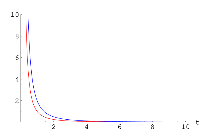
Figure 1: Plot of the solutions (85) in the inflationary regime (case $r=0.01$). The solid curve represents the $\Psi/\Psi_{0}$ the dashed one represents $\Delta/\Psi_{0}$.

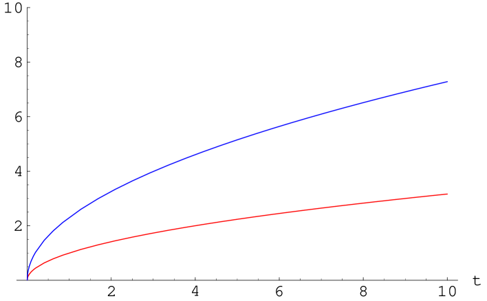
Figure 2: Plot of the solutions (85) for the case $r=-5$. The solid curve represents the $\Psi/\Psi_{0}$ the dashed one represents $\Delta/\Psi_{0}$.

The consequence of a growing mode on super-horizon scales during inflation suggests that there is a deviation from scale invariance for large $k$. As a consequence, any observed deviation from scale invariance on these scales could be used to constrain these models.

If we consider a Friedmann regime $(-4.73<r<-3.69,-1.27<r<-0.81)$, the perturbations on large scale grow as if the effective fluid was a form of standard matter. For example, supposing that the expansion of the background follows the standard behaviour $a\propto t^{2/3}$, which corresponds to $r\approx-4.17$, the parameter $p(r)$ of the scalar field is $\approx 3.6$, and in this case $w\approx 0$. If we choose $r=-4$, we would have a radiation-like effective fluid etc. This is means that a non-minimally coupled scalar field in a Friedmann regime can mimic baryonic fluids, but do not necessarily interact with photons via Thompson scattering.

Another curious behaviour in the Friedmann regime is that, for $(-4.73<r<-4.17,-1.07<r<-1.27)$, the perturbations are effectively frozen. This feature is very important when one makes the transition from perturbations seeded in the early universe to the matter power spectrum (if we take $\phi$ to correspond to the inflaton), and in general will affect the spectrum of scalar perturbations in the matter dominated era.

Finally, from the above equation we can also obtain the behaviour of the Newtonian potential $\Phi_{N}$:

$$\Phi_{N} = \frac{r^{2}\,\left(3+r\right)^{3}\,\left(6+5\,r\right)}{18\,\left(12+r\,\left(6+r\right)\right)\,\left(6+r\,\left(9+2\,r\right)\right)}\;C$$ (87)

$$+ \frac{2}{3}\;\frac{\left(3+r\right)\,\left(6+5\,r\right)}{6+r\,\left(9+2\,r\right)}\;{\alpha}^{2}\;\Delta_{0}\;t^{\frac{12+6r+r^{2}}{r(3+r)}}\;.$$

As in the minimally coupled case, $\Phi$ has a constant mode, but unlike the minimally coupled case, the other mode is not necessarily decreasing. In fact, the exponent $\displaystyle{\frac{12+6r+r^{2}}{r(3+r)}}$ is negative only if $-3<r<0$ (see Figure 3). This means that, when $r$ is outside the above interval, the gravitational potential increases in time so that the rate at which the perturbations grow is faster than in the case for a minimally coupled scalar field.

Figure 3: Plot of the exponent of the non-constant mode in (87)

VI Summary and Conclusions

In this paper we have developed the theory of cosmological perturbations of a FLRW background for a generic scalar-tensor theory of gravity in vacuum. Our analysis is based on the fact that the field equations of a scalar-tensor theory in vacuum can be recast in a form that resembles the standard Einstein theory, in which an effective fluid is present. This effective fluid is perfect in the background (like in the case of a minimally coupled scalar field), but it is imperfect in the perturbed universe. This is due to the peculiar form of the heat flux and the anisotropic pressure that depend on the acceleration and the shear as a result of the non-minimal coupling $F$.

As in bi:peterscalar , given our choice of $u^{a}$, the perturbations can be characterized using the variables $\mathcal{D}_{a}=\mu^{-1}a\tilde{\nabla}_{a}\mu$, $C_{a}=a^{3}\tilde{\nabla}_{a}\tilde{R}$ and $\Psi_{a}=\psi^{-1}a\tilde{\nabla}_{a}\psi$. The first one represents the density perturbation of the effective fluid; the second one, the projected gradient of the 3-curvature scalar of the $\phi=constant$ surfaces respectively; and the third one represents the inhomogeneities of the scalar field. Note that, due to the fact that in our frame $\tilde{\nabla}_{a}\phi=0$, this variable depends on the momentum $\psi$.

The three variables above are connected to each other via the constraint (III.2.2). In the minimally coupled case such constraint reduce to a proportionality relation between $\mathcal{D}_{a}$ and $\Psi_{a}$ and is used to eliminate the variable $\Psi_{a}$. However, in our case $\Psi_{a}$ and $\mathcal{D}_{a}$ have a rather different meaning and different relevance depending on the problem one wishes to solve. There can be cases in which the the perturbations of the effective fluid have a different impact on the matter perturbation and it is more useful to deal with $\mathcal{D}_{a}$ than $\Psi_{a}$.

Once we have chosen the perturbation variables it is relatively easy (although rather long!) to derive their evolution equations. These equation can be simplified if we consider spacetimes that do not differ too much from the background. In fact, in this case one can use the a linearization procedure based on the structure of the background to completely drop the interaction terms.

In this paper, we limited ourselves to analyze spherically symmetric clumping. This has been done by considering only the projected divergence of the variables above. The equations for these variables describe the evolution of scalar perturbations in a general scalar-tensor theory of gravity in vacuum. They are valid also for any spatial geometry and can be used to analyse the perturbations in any scalar - field - dominated universe models (not necessarily inflationary).

As an example we used a coupling, a potential and a background solution obtained in the framework of the Noether Symmetry approach bi:salvreview . We were able to solve the perturbation equations exactly for this background in the long wavelength limit. Our solution reveals that there exist power law inflation regimes in which the scalar field perturbations grow instead of being dissipated. Such a behaviour will affect the matter power spectrum, and potentially break scale invariance. However, this conclusion depends strictly on the behaviour of the perturbations on sub-horizon scales, which requires a complete analysis of the perturbation equations for all scales.

Also, we found that in “Friedmann regimes” the effective fluid associated with a non-minimally coupled scalar field is able to mimic a standard perfect fluid that does not necessarily interact with photons. The perturbations of this fluid grow for most of the values of $r$ associated to a Friedmann evolution, but there are also cases in which the super-horizon perturbations are effectively frozen, i.e., their growth rate is slower than the expansion rate, thereby differing significantly from the standard gravitational instability picture.

Finally, we derived the evolution of the gauge invariant version of the Newtonian potential $\phi_{N}$. As in the case of a minimally couple scalar field, $\phi_{N}$ contains a constant mode. However, unlike the minimally coupled case, it also admits a second mode that is not necessarily decaying and this again modifies the standard picture.

In conclusion, our preliminary results reveal that the presence of a non-minimal coupling has unexpected and interesting effects on the evolution of the long wavelength scalar perturbations. An analysis of the full perturbation spectrum will clarify further on these properties and will be presented in a forthcoming paper.

VII Acknowledgements

This work was supported by the National Research Foundation (South Africa) and the Ministrero deli Affari Esteri- DIG per la Promozione e Cooperazione Culturale (Italy) under the joint Italy/South Africa science and technology agreement.

Appendix A Coefficients of the perturbation equations

For sake of simplicity in the main body of the paper we give here the expressions of the coefficient of the equations (IV.1). All the quantities appearing in these coefficients are meant to be the background ones.

$$\mathcal{A}_{\Delta}(t) = \frac{9\,K\,\dot{F}^{2}\,\left(F\,\left(1+w\right)\,\mu+\Theta\,\dot{F}\right)}{2\,F\,a^{4}\,\left(1+w\right)\,\Theta\,{\mu}^{2}\,\left(2\,F\,{\psi}^{2}+3\,\dot{F}^{2}\right)}$$

$$+ \frac{3\,F\,\left(1+w\right)\,\mu\,\psi^{2}+\Theta\,\dot{F}\,\left(2\,{\psi}^{2}-3\,F\,\left(1+w\right)\,\mu-2\,\Theta\,\dot{F}+3\,\ddot{F}\right)}{2\,a^{2}\,\Theta\,\mu\,\left(2\,F\,{\psi}^{2}+3\,\dot{F}^{2}\right)}$$

$$\mathcal{B}_{\Delta}(t) = \frac{K\,\dot{F}^{2}\,\left[3\,F\,\mu\,\left(2\,w\,{\Theta}^{2}-3\,\left(1+w\right)\,\mu\right)-6\,{\Theta}^{2}\,{\psi}^{2}+\Theta\,\dot{F}\,\left(2\,{\Theta}^{2}\,-9\,\mu\right)-6\,{\Theta}^{2}\,\ddot{F}\right]}{F\,a^{2}\,\left(1+w\right)\,\Theta\,{\mu}^{2}\,\left(2\,F\,{\psi}^{2}+3\,\dot{F}^{2}\right)}$$ (88)

$$+ \frac{3\,F\,\psi^{2}\,\left(2\,w\,{\Theta}^{2}-3\,\left(1+w\right)\,\mu\right)+2\,\Theta\,F\,\dot{F}\,\left(2\,{\Theta}^{2}+6\,\mu+9\,w\,\mu\right)}{3\,\Theta\,\left(2\,F\,{\psi}^{2}+3\,\dot{F}^{2}\right)}$$

$$- \frac{\Theta\,\dot{F}\,\left(6\,{\psi}^{2}-3\,\dot{F}\,\left(1+3\,w\right)\,\Theta\,\psi+9\,\ddot{F}\right)}{3\,\Theta\,\left(2\,F\,{\psi}^{2}+3\,\dot{F}^{2}\right)}$$

$$\mathcal{C}_{\Delta}(t) = \frac{6\,\Theta\,\left({\Theta}^{2}+\mu+3\,w\,\mu\right)\,\dot{F}^{2}-\left(4\,{\Theta}^{2}+3\,\mu+9\,w\,\mu\right)\,\dot{F}\psi^{2}-6\,\Theta\,\ddot{F}\psi^{2}}{3\,\mu\left(2\,F\,{\psi}^{2}+3\,\dot{F}^{2}\right)}$$ (89)

$$- \frac{2\,K\,\Theta\,\dot{F}^{2}\,\left[4\,\Theta\,\dot{F}-3\,\psi^{2}\,\left(2+F^{\prime\prime}\right)\right]}{F\,a^{2}\,\left(1+w\right)\,{\mu}^{2}\,\left(2\,F\,{\psi}^{2}+3\,\dot{F}^{2}\right)}$$

$$\mathcal{D}_{\Delta}(t) = -\frac{\dot{F}^{3}}{2\,{\mu}^{2}\,F\,a^{2}\,\left(1+w\right)\,\left(2\,F\,{\psi}^{2}+3\,\dot{F}^{2}\right)}$$

$$\mathcal{E}_{\Delta}(t) = \frac{\dot{F}^{3}\,\left(2\,{\Theta}^{2}+3\,\mu\right)+6\,\Theta\,\dot{F}^{2}\,\left(F\,w\,\mu-{\psi}^{2}-\ddot{F}\right)}{3\,F\,\left(1+w\right)\,{\mu}^{2}\,\left(2\,F\,{\psi}^{2}+3\,\dot{F}^{2}\right)}$$

$$\mathcal{F}_{\Delta}(t) = \frac{6\,F^{2}\,\left(1+w\right)\,\mu\,\dot{F}\,\psi^{2}+6\,F\,\Theta\,\dot{F}^{2}\,\left(2\,{\psi}^{2}-F\,\left(1+w\right)\,\mu\right)}{3\,F^{2}\,\left(1+w\right)\,{\mu}^{2}\,\left(2\,F\,{\psi}^{2}+3\,\dot{F}^{2}\right)}$$ (90)

$$+ \frac{\dot{F}^{3}\,\left(9\,F\,\left(1+w\right)\,\mu+12\,\Theta\,\dot{F}-8\,F\,{\Theta}^{2}\right)+6\,F\,\Theta\dot{F}^{2}\,\psi^{2}\,F^{\prime\prime}}{3\,F^{2}\,\left(1+w\right)\,{\mu}^{2}\,\left(2\,F\,{\psi}^{2}+3\,\dot{F}^{2}\right)}$$

$$\mathcal{A}_{C}(t) = \frac{3F\,\mu\,\left(1+w\right)+3\Theta\,\dot{F}}{\mu\,F\,a^{2}\,\Theta\,\left(1+w\right)}$$ (91)

$$\mathcal{B}_{C}(t) = \frac{6\,F\,\mu\,\left(2\,w\,{\Theta}^{2}-3\,\left(1+w\right)\,\mu\right)-12\,{\Theta}^{2}\,{\psi}^{2}+2\Theta\,\dot{F}\,\left(2\,{\Theta}^{2}-9\,\mu\right)-12\,{\Theta}^{2}\,\ddot{F}}{3\,F\,\left(1+w\right)\,\Theta\,\mu}$$ (92)

$$\mathcal{C}_{C}(t) = \frac{4\,\Theta\,\left(3\,\psi^{2}\,\left(2+F^{\prime\prime}\right)-4\,\Theta\,\dot{F}\right)}{3\,\mu\,F\,\left(1+w\right)}$$ (93)

$$\mathcal{D}_{C}(t) = -\frac{\psi\,F^{\prime}}{3\,F\,\mu\left(1+w\right)}$$ (94)

$$\mathcal{E}_{C}(t) = \frac{2\,a^{2}\,\dot{F}\,\left(2\,{\Theta}^{2}+3\,\mu\right)+12\,a^{2}\,\Theta\,\left(F\,w\,\mu-{\psi}^{2}-\ddot{F}\right)}{9\,\mu\,F\,\left(1+w\right)}$$ (95)

$$\mathcal{F}_{C}(t) = \frac{2\,a^{2}\,\left[F\,\dot{F}\,\left(9\,\left(1+w\right)\,\mu-8\,{\Theta}^{2}\right)+12\,\Theta\,\dot{F}^{2}+6\,F\,\Theta\,\psi^{2}\,\left(2+F^{\prime\prime}\right)\right]}{9\,\mu\,F^{2}\,\left(1+w\right)}$$ (96)

$$\mathcal{A}_{\Psi}(t) = -\frac{9\,K\,\dot{F}\,\left(F\,\left(1+w\right)\,\mu+\Theta\,\dot{F}\right)}{2\,a^{4}\,\left(1+w\right)\,{\Theta}^{2}\,\mu\,\left(2\,F\,\psi^{2}+3\,\dot{F}^{2}\right)}$$ (97)

$$+ \frac{6\,\mu\,\Theta\,F^{2}\,\left(1+w\right)+\dot{F}\,\left[F\left(4\,{\Theta}^{2}+9\,\left(1+w\right)\,\mu\right)+6\,\Theta\,\dot{F}\right]-6\,F\,\Theta\,\ddot{F}}{4\,a^{2}\,{\Theta}^{2}\,\left(2\,F{\psi}^{2}+3\,\dot{F}^{2}\right)}$$

$$\mathcal{B}_{\Psi}(t) = -\frac{4\,\mu\,F^{2}\,\Theta\,\left(2\,{\Theta}^{2}+6\,\mu+9\,w\,\mu\right)-18\,\mu\,F\,\Theta\,\ddot{F}}{6\,{\Theta}^{2}\,\left(2\,F{\psi}^{2}+3\,\dot{F}^{2}\right)}$$ (98)

$$+ \frac{3\,\mu\,\dot{F}\,\left(2\,F\,{\Theta}^{2}+9\,F\,\left(1+w\right)\,\mu+6\,\Theta\,\psi\,F^{\prime}\right)}{6\,{\Theta}^{2}\,\left(2\,F{\psi}^{2}+3\,\dot{F}^{2}\right)}$$

$$- K\left\{\frac{\,F^{\prime}\,\left(3\,F\,\mu\,\left(2\,w\,{\Theta}^{2}-3\,\left(1+w\right)\,\mu\right)-6\,{\Theta}^{2}\,{\psi}^{2}\right)}{a^{2}\,\left(1+w\right)\,{\Theta}^{2}\,\mu\,\psi\,\left(2\,F+3\,{F^{\prime}}^{2}\right)}\right.$$

$$+ \left.\frac{\Theta\,\dot{F}^{2}\,\left(2\,{\Theta}^{2}\,\psi-9\,\mu\,\psi\right)-6\,F^{\prime}\,{\Theta}^{2}\,\ddot{F}}{a^{2}\,\left(1+w\right)\,{\Theta}^{2}\,\mu\,\left(2\,F\,\psi^{2}+3\,\dot{F}^{2}\right)}\right\}$$

$$\mathcal{C}_{\Psi}(t) = \frac{2\,K\,\dot{F}\,\left(4\,\Theta\,\dot{F}-3\,\psi^{2}\,\left(2+F^{\prime\prime}\right)\right)}{a^{2}\,\left(1+w\right)\,\mu\,\left(2\,F\,\psi^{2}+3\,\dot{F}^{2}\right)}$$ (99)

$$- \frac{F\,\psi^{2}\,\left[2\,{\Theta}^{2}-3\,\left(\mu+3\,w\,\mu\right)\right]+3\,\Theta\,\left(4\,F\,\psi\,\psi^{\prime}+3\,\dot{F}^{2}\,\Theta\right)}{3\,\Theta\,\left(2\,F\,\psi^{2}+3\,\dot{F}^{2}\right)}$$

$$+ \frac{3\,\Theta\,\dot{F}\,\left(2\,F\,\left({\Theta}^{2}+\mu+3\,w\,\mu\right)+3\,\ddot{F}\right)}{3\,\Theta\,\left(2\,F\,\psi^{2}+3\,\dot{F}^{2}\right)}$$

$$\mathcal{D}_{\Psi}(t) = \frac{\dot{F}^{2}}{2\,\mu\,a^{2}\,\Theta\,\left(1+w\right)\,\left(2\,F\,{\psi}^{2}+3\,\dot{F}^{2}\right)}$$ (100)

$$\mathcal{E}_{\Psi}(t) = \frac{6\,\Theta\,\dot{F}\,\left({\psi}^{2}-F\,w\,\mu+\ddot{F}\right)-\dot{F}^{2}\,\left(2\,{\Theta}^{2}+3\,\mu\right)}{3\,\Theta\,\mu\,\left(1+w\right)\,\left(2\,F\,{\psi}^{2}+3\,\dot{F}^{2}\right)}$$ (101)

$$\mathcal{F}_{\Psi}(t) = \frac{2\,\dot{F}\,\left[3\,F\,\left(F\,\left(1+w\right)\,\mu-2\,{\psi}^{2}\right)+4\,F\,\Theta\,\dot{F}-6\,\dot{F}^{2}-3\,F\,\psi^{2}\,F^{\prime\prime}\right]}{3\,\mu\,F\,\left(1+w\right)\,\left(2\,F\,{\psi}^{2}+3\,\dot{F}^{2}\right)}$$ (102)

References

References

- (1) For an updated review see for example T. Padmanabhan, “Cosmological constant: The weight of the vacuum,” Phys. Rept. 380 (2003) 235 [arXiv:hep-th/0212290].
- (2) R. R. Caldwell, R. Dave and P. J. Steinhardt, “Cosmological Imprint of an Energy Component with General Equation-of-State,” Phys. Rev. Lett. 80 (1998) 1582 [arXiv:astro-ph/9708069].
- (3) N. Ogawa, “A note on classical solution of Chaplygin gas as d-branes,” Phys. Rev. D 62 (2000) 085023 [arXiv:hep-th/0003288];A. Y. Kamenshchik, U. Moschella and V. Pasquier, “An alternative to quintessence,” Phys. Lett. B 511 (2001) 265 [arXiv:gr-qc/0103004].
- (4) R. R. Caldwell, “A Phantom Menace?,” Phys. Lett. B 545 (2002) 23 [arXiv:astro-ph/9908168].
- (5) J. F. Donoghue, “General relativity as an effective field theory: The leading quantum corrections,” Phys. Rev. D 50 (1994) 3874 [arXiv:gr-qc/9405057].
- (6) G. Lessner, Unified field theory on the basis of the projective theory of relativity, Phys. Rev. D25 (1982) 3202; ibid D27 (1982) 1401.
- (7) Fuji, Y., Maeda, K., “The scalar-tensor theory of gravitation” (Cambridge Univ. Press, 1998) Cambridge.
- (8) M. Green, J. Schwarz and E. Witten, Superstring theory, Vol. 1 & 2(Cambridge Univ. Press, 1987); E. Kiritsis, Introduction to superstring theory, Leuven notes in math. and theor. physics, 9 (1997), hep-th/9709062; J. Polchinski, String Theory, Vol. I & II (Cambridge Univ. Press, 1998).
- (9) T. Chiba, “Scalar-tensor gravity in two 3-brane system,” Phys. Rev. D 62 (2000) 021502(R) [arXiv:gr-qc/0001029].
- (10) Ellis, G. F. R. 1973, Relativistic cosmology, in Cargese Lectures in Physics, Volume 6, Ed. Schatzmann, E. (Gordon and Breach), 1.
- (11) M. Bruni, G. F. R. Ellis and P. K. S. Dunsby, “Gauge invariant perturbations in a scalar field dominated universe,” Class. Quant. Grav. 9 (1992) 921.
- (12) Ellis, G. F. R., Bruni, M. and Hwang, J. Covariant and gauge independent perfect fluid Robertson-Walker perturbations Phys. Rev. D 40 1819 (1989); ibid , Density gradient - vorticity relation in perfect fluid Robertson - Walker perturbations.
- (13) D. La and P. J. Steinhardt, “Extended Inflationary Cosmology,” Phys. Rev. Lett. 62 (1989) 376 [Erratum-ibid. 62 (1989) 1066].
- (14) P. J. Steinhardt and F. S. Accetta, “Hyperextended Inflation,” Phys. Rev. Lett. 64 (1990) 2740.
- (15) Hawking, S. W. 1966, Perturbations of an expanding universe, Ap. J. 145, 544.
- (16) Bardeen, J. M. , Gauge invariant cosmological perturbations, Phys. Rev. D, 22, 1982 (1980).
- (17) Kodama, H. and Sasaki, M. , Cosmological perturbation theory, KS, Prog. Theor. Phys. 78, 1 (1984).
- (18) V. F. Mukhanov, H. A. Feldman and R. H. Brandenberger, “Theory Of Cosmological Perturbations. Part 1. Classical Perturbations. Part 2. Quantum Theory Of Perturbations. Part 3. Extensions,” Phys. Rept. 215 203 (1992).
- (19) S. Capozziello, R. De Ritis, C. Rubano, M. Demianski, “Cosmological perturbations in exact Noether background solutions,” Phys. Rev. D 52 3288 (1995).
- (20) J. C. Hwang, “Cosmological Perturbations In Generalized Gravity Theories: Formulation,” Class. Quant. Grav. 7 1613 (1990); J. C. Hwang, “Cosmological Perturbations In Generalized Gravity Theories: Solutions,” Phys. Rev. D 42 (1990) 2601; J. C. Hwang, “Perturbations of the Robertson-Walker space - Multicomponent sources and generalized gravity,” Astrophys. J. 375 443 (1991); J. c. P. Hwang, “Unified Analysis of Cosmological Perturbations in Generalized Gravity,” Phys. Rev. D 53 (1996) 762 [arXiv:gr-qc/9509044]; J. c. P. Hwang and H. Noh, “Cosmological perturbations in generalized gravity theories,” Phys. Rev. D 54 (1996) 1460; J. c. Hwang, “Cosmological perturbations in generalized gravity theories: Conformal transformation,” Class. Quant. Grav. 14 (1997) 1981 [arXiv:gr-qc/9605024]; J. C. Hwang, “Quantum fluctuations of cosmological perturbations in generalized gravity,” Class. Quant. Grav. 14 (1997) 3327 [arXiv:gr-qc/9607059]; J. Hwang, “Cosmological structures in generalized gravity,” arXiv:gr-qc/9711086; J. C. Hwang, “The origin of structures in generalized gravity,” Gen. Rel. Grav. 30 (1998) 545 [arXiv:gr-qc/9711067]; H. Noh and J. C. Hwang, “Cosmological perturbations in generalized gravity theories,” Mod. Phys. Lett. A 19 (2004) 1203;
- (21) C. Brans and H. Dicke,“Mach’s Principle And A Relativistic Theory Of Gravitation”, Phys. Rev. 124, 925 (1961)
- (22) See for example E. Elizalde, S. Nojiri and S. D. Odintsov, “Late-time cosmology in (phantom) scalar-tensor theory: Dark energy and the cosmic speed-up,” Phys. Rev. D 70 (2004) 043539 [arXiv:hep-th/0405034].
- (23) M. Demianski, E. Piedipalumbo, C. Rubano and C. Tortora, “Accelerating universe in scalar tensor models: Confrontation of theoretical predictions with observations”, Astron. Astrophys. 454 (2006) 55 [arXiv:astro-ph/0604026]; ibid “Exact general solution for scalar tensor theories: theory and fit to the observations”, in preparation
- (24) Wald, R. M. 1984, General Relativity (The University of Chicago Press).
- (25) Madsen, M. S. 1988, Scalar fields in curved spacetimes, Class. Quantum Grav. 5, 627.
- (26) King A. R. and Ellis G. F. R. 1973, Tilted homogeneous cosmological models, Commun. Math. Phys. 31 209
- (27) Bruni, M., Dunsby, P. K. S. and Ellis, G. F. R. 1991, Cosmological perturbations and the physical meaning of gauge-invariant variables, PAPER I, to appear in Ap. J.
- (28) Ellis G F R, Bruni M 1989, Covariant and gauge invariant approach to density fluctuations, Phys Rev D 40 1804
- (29) Stewart, J. M. 1990, Perturbations of Friedmann - Robertson - Walker cosmological models, Class. Quantum Grav. 7, 1169.
- (30) J. M. Bardeen, P. J. Steinhardt and M. S. Turner, “Spontaneous Creation Of Almost Scale - Free Density Perturbations In An Inflationary Universe,” Phys. Rev. D 28 (1983) 679.
- (31) Ellis, G. F. R. 1971, in General Relativity and Cosmology, Proceedings of XLVII Enrico Fermi Summer School, ed Sachs, R. K. (New York Academic Press).
- (32) S. Capozziello, R. De Ritis, C. Rubano and P. Scudellaro, “Noether symmetries in cosmology,” Riv. Nuovo Cim. 19N4 (1996) 1.
- (33) R. de Ritis and A. A. Marino, “Effective cosmological ’constant’ and quintessence,” Phys. Rev. D 64 (2001) 083509 [arXiv:astro-ph/0007128].