Entropy of gravitating systems: scaling laws versus radial profiles

Abstract

Through the consideration of spherically symmetric gravitating systems consisting of perfect fluids with linear equation of state constrained to be in a finite volume, an account is given of the properties of entropy at conditions in which it is no longer an extensive quantity (it does not scale with system’s size). To accomplish this, the methods introduced by Oppenheim Oppen2 to characterize non-extensivity are used, suitably generalized to the case of gravitating systems subject to an external pressure. In particular when, far from the system’s Schwarzschild limit, both area scaling for conventional entropy and inverse radius law for the temperature set in (i.e. the same properties of the corresponding black hole thermodynamical quantities), the entropy profile is found to behave like $1/r$, being $r$ the area radius inside the system. In such circumstances thus entropy heavily resides in internal layers, in opposition to what happens when area scaling is gained while approaching the Schwarzschild mass, in which case conventional entropy lies at the surface of the system. The information content of these systems, even if it globally scales like the area, is then stored in the whole volume, instead of packed on the boundary.

I Introduction

The study of the connection between entropy and gravity, performed even simply at a classical level, has deserved in recent years very interesting results. Examples have been found in which the conventional (as opposed to black hole) entropy of gravitating systems scales like their area and the temperature like $1/R$ (being $R$ their area radius), that is the same as the celebrated laws of black hole entropy and temperature if area and radius refer to horizon hawking ; bekenstein .

Black hole properties are apparent at a semi-classical level in which quantum fields live in a continuous curved spacetime, describing gravity; these properties moreover, in particular the area scaling law of black hole entropy, are considered to give hints or constraints on a fundamental description of spacetime itself, possibly at a quantum level, of a holografic nature thooft ; susskind . Now, the fact that purely classical systems can exhibit analogous scaling laws in the corresponding conventional thermodynamical quantities is intriguing. The study of these systems could shed light on what in the area scaling property of black hole entropy truly points to a fundamental origin.

In banks gravitating systems consisting of perfect fluids with linear equation of state $p=\kappa\rho$, with $p$ and $\rho$ the pressure and energy density and $\kappa$ a (non-negative) constant, have been considered. The authors have found the remarkable property that for the stiffest case compatible with causality, namely the $\kappa=1$ case (see zeldovich ), the equilibrium configurations can exhibit area scaling of their entropy, as well $1/R$ scaling of their temperature, suggesting a possible connection between holografy and causality. This recalls the formulation of the holographic principle, as given by bousso , which has causality built-in. In Oppen1 , the entropy of a spherically symmetric gravitating system in equilibrium has been shown to become area scaling as the radius approaches the Schwarzschild value; in this limit the total entropy of the body is accounted for only by the entropy of the more external spherical shells.

In general when gravity enters the game, extensivity of entropy is lost even if, by the equivalence principle, it is mantained locally. In Oppen2 a method has been introduced to study the degree of non-extensivity of entropy (its scaling behaviour with system’s size) for systems with long range interactions (other approaches to non-extensivity, trying to characterize and understand it outside standard thermodynamics, use Tsallis entropy Tsallis ; see also Renyi ). Applying this method to a particular system consisting of a spherically symmetric distribution of perfect fluid with constant density, it appears that at increasing $M/R$ ($M$ is the mass, or mass-energy, as spelled out in Wheeler , known also as ADM mass) entropy starts going towards area scaling, with an increasing contribution from external layers (the limit $R=2M$ is however not reachable as equilibrium is possible only if $R\geq(9/4)M$ (see, for instance, Wheeler )), in agreement with what expected from Oppen1 . The idea in the present paper is to go back to the systems banks , known to reach conditions with area scaling of entropy, and to investigate, through a generalization of the method introduced in Oppen2 , the dependence of non-extensivity on $M/R$ as well to study the evolution of the entropy profile.

The paper is organized as follows. In section II we examine the equilibrium configurations of the fluids under consideration first under conditions in which they are unconstrained and next when they are instead constrained to be in a fixed volume. For these latter conditions in section III we try to characterize the degree of non-extensivity of the systems following the approach Oppen2 , trying to extend it to cover the case in which an external pressure is applied, i.e. our case. A global temperature is introduced and an expression is found that for each $\kappa$ gives the degree of non-extensivity of the entropy of the system for assigned (central) energy density and size. In section IV first we use this result to investigate the scaling laws for entropy; next the scaling laws for global temperature are also derived and, finally, the entropy radial profiles are considered, in their relation with the scaling laws of entropy, in particular for the most interesting case $\kappa=1$. We conclude with a summary of our results in section V.

II Equilibrium configurations for linear perfect fluids

As in banks , let us consider a perfect fluid at thermodynamic equilibrium with linear equation of state

$$p=\kappa\rho,$$ (1)

where $\rho$ and $p$ are respectively the energy density and pressure in the rest frame of the fluid element; $\kappa$ is a constant with $0\leq\kappa\leq 1$ where, as said, $\kappa=1$ corresponds to the stiffest conditions compatible with causality. The stress-energy tensor is

$$T_{\alpha\beta}=(\rho+p)u_{\alpha}u_{\beta}+pg_{\alpha\beta},$$ (2)

where $u_{\alpha}$ is the fluid element 4-velocity and $g_{\alpha\beta}$ is the metric tensor. In the case of static equilibrium configurations (necessarily with spherical symmetry), from (1) and (2) Einstein field equations in Schwarzschild coordinates can be written

$$\frac{h^{\prime}}{rh^{2}}+\frac{h-1}{hr^{2}}=8\pi\rho\ \ \ \ \qquad\qquad\qquad\qquad\quad\qquad\qquad(tt)$$

$$\frac{f^{\prime}}{rfh}-\frac{h-1}{hr^{2}}=8\pi p\ \ \ \qquad\qquad\qquad\qquad\quad\qquad\qquad(rr)$$ (3)

$$\frac{f^{\prime}}{rfh}-\frac{h^{\prime}}{rh^{2}}+\frac{1}{\sqrt{fh}}\left(\frac{f^{\prime}}{\sqrt{fh}}\right)^{\prime}=16\pi p\ \ \ \qquad\qquad(\theta\theta)=(\phi\phi),$$

where the derivative symbol means derivative with respect to radial coordinate (area radius) $r$ and where the metric is

$$ds^{2}=-f(r)\ dt^{2}+h(r)\ dr^{2}+r^{2}\ d\Omega^{2},$$ (4)

with $f$ and $h$ two non-negative functions of $r$, to be determined.

The properties of the solutions to these equations are known since a long time Chandra . The equilibrium configurations are completely determined by the equation of state (1); they can be derived solving directly the Tolman-Oppenheimer-Volkoff equation (Tolman1939 ; OV and Chandra ). Aiming however at obtaining entropy profiles, we want to stress the dependence on temperature. We choose then to solve equations (II) inserting explicitly this dependence since start. For static gravitational fields, Tolman relation Tolman1930 prescribes that $T\sqrt{-g_{00}}$ be constant throughout the system, where $T$ is the temperature in the rest frame of the fluid element. This means for us that

$$T(r)\sqrt{f(r)}=const.$$ (5)

For our fluid, thermodynamics gives the following scaling laws banks2 ; banks3

$$\rho\propto T^{(\kappa+1)/\kappa},$$ (6)

$$s\propto T^{1/\kappa},$$ (7)

with $s$ the entropy density. The proportionality constants depend on the particular realization of the fluid. Applying these scaling laws locally throughout our system (equivalence principle), from equation (5) we have thus

$$\rho(r)f^{\frac{\kappa+1}{2\kappa}}(r)=const\equiv\frac{C}{8\pi},$$ (8)

with $C$ some constant with the dimensions of energy density (length^-2 in geometrized units). Note that while the value of $C$ depends on the chosen unit for length, the quantities $\rho/C$ and $r\sqrt{C}$ are dimensionless.

Making use of (8), the first and the second of equations (II) become

$$\frac{C}{f^{\frac{\kappa+1}{2\kappa}}}=\frac{h^{\prime}}{rh^{2}}+\frac{h-1}{hr^{2}}$$ (9)

$$\kappa\frac{C}{f^{\frac{\kappa+1}{2\kappa}}}=\frac{f^{\prime}}{rfh}-\frac{h-1}{hr^{2}},$$ (10)

while the third, as can be verified (and as noticed in photonstars , in the case of a photon gas), is always identically satisfied if equations (9-10) are satisfied, as a confirmation of Tolman result.

Before we start to solve these coupled differential equations, let us study some general characteristics which the solutions $f(r)$ and $h(r)$ should satisfy. $h(r)$ can be put in the form

$$h(r)=\frac{1}{1-2m(r)/r},$$ (11)

(see for example Wheeler ) with $m(r)$ given by

$$m(r)=\int_{0}^{r}{4\pi{\tilde{r}}^{2}\rho({\tilde{r}})d{\tilde{r}}}=\frac{C}{2}\int_{0}^{r}{\frac{{\tilde{r}}^{2}}{f^{g}({\tilde{r}})}d{\tilde{r}}},$$ (12)

that is, $m(r)$ is the ADM mass inside $r$. Here we have introduced the function

$$g(\kappa)=\frac{\kappa+1}{2\kappa},$$ (13)

so that $g(\kappa)$ is monotonically decreasing in the relevant range $0<\kappa\leq 1$, with $g(\kappa)\geq 1$ and $g(\kappa)\rightarrow\infty$ for $\kappa$ approaching 0. The cases of perfect fluids with $\kappa=0$ (dust), $\kappa=1/3$ (blackbody radiation) and $\kappa=1$ (stiff matter) correspond respectively to $g=\infty$, $g=2$ and $g=1$. In the following we will often refer to $g$ instead of $\kappa$.

For each allowed equilibrium configuration, in the limit $r\rightarrow 0$

$$m(r)\simeq\frac{4}{3}\pi r^{3}\rho(0),$$ (14)

so that $m(r)/r\rightarrow 0$. This implies $h(0)=1$ for each solution with $\rho(0)$ finite. As regards $f$, from (8) we have

$$\rho(0)f^{g}(0)=\frac{C}{8\pi},$$ (15)

so that finite $\rho(0)$ implies a non zero $f(0)$. Taking the derivative of (11) and using (14) and (15), in the limit $r\rightarrow 0$ we have $h^{\prime}(r)\simeq\frac{16}{3}\pi\rho(0)r$ and $f^{\prime}(r)\simeq rf(0)\frac{16}{3}\pi\frac{g+1}{2g-1}\rho(0)$, so that $h^{\prime}(0)=0$ and $f^{\prime}(0)=0$.

We want now to solve equations (9-10). We can write equation (10) as

$$h=(2g-1)\frac{f^{g-1}(f+rf^{\prime})}{Cr^{2}+(2g-1)f^{g}}$$ (16)

and, substituting this expression of $h$ in equation (9), we obtain

$$f^{\prime\prime}=\frac{2(g+1)Crf^{2}+3gCr^{2}ff^{\prime}-2(2g-1)f^{g+1}f^{\prime}+gCr^{3}{f^{\prime}}^{2}}{Cr^{3}f+(2g-1)rf^{g+1}}$$ (17)

so that equations (16-17) are equivalent to the starting equations (9-10). Using, in addition, the previous results about the behaviour of $f$ near the origin, the problem is thus reduced to find the solutions $f$ of the second order equation (17) with initial conditions

$$f(0)=\Big{(}\frac{C}{8\pi\rho(0)}\Big{)}^{1/g}; \qquad\qquad f^{\prime}(0)=0.$$ (18)

For assigned $g$, for each choice of the pair $C$, $\rho(0)$ we have a solution $f(r)$. Note however from equation (8) that physical configurations $\rho=\rho(r)$ depend only on the ratio $C/f^{g}$ and not on $C$ and $f$ separately. This implies that for any chosen $\rho(0)$, the (infinite number of) solutions $f$ that we find when $C$ is varied, correspond always to the same physical configuration $\rho=\rho(r)$. For each $g$, to fix $\rho(0)$ corresponds to uniquely fix the physical configuration, irrespective of the separate values of $C$ and $f$. Without loss of generality we can then study the solutions to equation (17) for a single arbitrary choice of the value of $C$ ($\not=0$); let us put for simplicity $C=1$. All possible static configurations of our system are then in 1-1 correspondence with all the solutions $f$ of equation

$$f^{\prime\prime}=\frac{2(g+1)rf^{2}+3gr^{2}ff^{\prime}-2(2g-1)f^{g+1}f^{\prime}+gr^{3}{f^{\prime}}^{2}}{r^{3}f+(2g-1)rf^{g+1}}$$ (19)

with initial conditions

$$f(0)=\Big{(}\frac{1}{8\pi\rho(0)}\Big{)}^{1/g}, \qquad\qquad f^{\prime}(0)=0,$$ (20)

where $\rho(0)$ is any positive number and with $h$ given by (16). Due to (6), each specification of $\rho(0)$ is equivalent to a specification of the central temperature $T_{C}$.

Some symmetry considerations can now help to understand how the set of solutions $f$ (and $h$) is arranged. Consider the transformation

$$r\rightarrow{\tilde{r}}=\lambda r$$ (21)

$$f\rightarrow{\tilde{f}}=\lambda^{2/g}f.$$ (22)

We have

$${\tilde{f}}({\tilde{r}})=\lambda^{2/g}f({\tilde{r}}/\lambda)$$

or

$${\tilde{f}}(r)=\lambda^{2/g}f(r/\lambda)$$

and then

$${\tilde{f}}^{\prime}(r)=\lambda^{\frac{2}{g}-1}f^{\prime}(r/\lambda)$$

and

$${\tilde{f}}^{\prime\prime}(r)=\lambda^{\frac{2}{g}-2}f^{\prime\prime}(r/\lambda)$$

so that, if $f(r)$ is a given solution, ${\tilde{f}}(r)$ is also a solution, as can be easily verified going through equation (19). ${\tilde{f}}(r)$ is such that ${\tilde{f}}(0)=\lambda^{2/g}f(0)$. On the other hand we know that, starting from a given solution $f_{1}$, we can obtain all solutions for the assigned $g$ if we change the initial conditions, $f_{1}(0)\rightarrow f_{\lambda}(0)=\lambda f_{1}(0)$, with $\lambda$ spanning all positive real values. Thus, in terms of an assigned solution $f_{1}(r)$, a function $f_{\lambda}$ is a solution if and only if

$$f_{\lambda}(r)=\lambda f_{1}(r/\lambda^{\frac{g}{2}})$$ (23)

with $\lambda>0$. For the solutions $h$ we obtain

$$h_{\lambda}(r)=h_{1}(r/\lambda^{\frac{g}{2}}),$$ (24)

where $h_{\lambda}(r)$ and $h_{1}(r)$ corresponds to $f_{\lambda}(r)$ and $f_{1}(r)$ through (16). We see that, from (8), the transformations we are considering are equivalent to say that equations (II) are invariant under the transformation banks ; sorkin ; bondi

$$r\rightarrow\lambda r$$

$$p\rightarrow p/\lambda^{2}$$ (25)

$$\rho\rightarrow\rho/\lambda^{2}.$$

Summing up, once we know the behaviour of solutions $f$ and $h$ for a given particular initial value $f(0)=a_{1}$ of $f$, arbitrarily fixed ($>0$), we can readily get the corresponding behaviours of the solutions for every other assigned initial value $a_{2}$. Let us study for simplicity the case $f(0)=1$, that is the solutions to (19) with initial conditions

$$f(0)=1; \qquad\qquad f^{\prime}(0)=0.$$ (26)

From numerical integration of equation (19) and from equation (16) we obtain the solutions $f$ and $h$ reported in Figures 1 and 2 for the cases $g=1,\ 2,\ 5$ (i.e. $\kappa=1,\ \frac{1}{3},\ \frac{1}{3^{2}}$).

Figure 1: $f$ versus $r$ for $\kappa=1,\ \frac{1}{3},\ \frac{1}{9}$ (highest: $\kappa=1$, lowest: $\kappa=\frac{1}{9}$) for initial conditions (26), see text.

Figure 2: $h$ versus $r$ for $\kappa=1,\ \frac{1}{3},\ \frac{1}{9}$ (highest: $\kappa=1$, lowest: $\kappa=\frac{1}{9}$) for initial conditions (26), see text.

The structure of the corresponding equilibrium configuration can be seen in Figures 3 and 4, that respectively report $\rho$ and $2m/r$, as a function of $r$, for the same chosen values of $g$. Our choice $C=1$ implies that $\rho$ and $r$ are given here respectively in units of $C$ and $C^{-1/2}$. From (8) and (23) the properties of $\rho$ for every other solution can readily be inferred. Note that $\rho(r)$ approaches asymptotically 0 as $r\rightarrow\infty$. This implies that for this configuration and, by scaling property (23), for every other solution, the radius of the system is infinite as expected. These radial profiles agree with the corresponding results reported in Chavanis within an extensive study of the conditions of general relativistic instability of finite spheres consisting of exactly the same fluids we are examining here.

Let us consider in some detail the functions $h$ and $2m/r$ (Figures 2 and 4). $h$ starts from 1 at $r=0$, and $2m/r$ from 0; they reach their maxima, after which they go towards their own limiting values photonstars ,

$$h(\infty)=2,\ \frac{7}{4},\ \frac{34}{25},$$ (27)

and

$$\left(\frac{2m}{r}\right)_{\infty}=\frac{1}{2},\ \frac{3}{7},\ \frac{9}{34},$$ (28)

respectively for $g=1,\ 2,\ 5$, shown in the Figures, with damped oscillations around them, in which both the amplitudes of the deviations from the limiting values as well their derivatives at any order reduce asymptotically to 0. Analytically both limiting values can easily be verified. In fact consider for example that from (11) we have

$$\frac{2m}{r}=\frac{h-1}{h}.$$ (29)

In equation (9) we see then that, at extremal points, that is when $r$ has values $r^{*}$ such that $h^{\prime}(r^{*})=0$ (that is $(2m(r)/r)^{\prime}_{r=r^{*}}=0$), we have

$$\frac{2m(r^{*})}{r^{*}}=\frac{{r^{*}}^{2}}{f^{g}(r^{*})}.$$ (30)

As extremal values tend to $(2m/r)_{\infty}$ when $r\rightarrow\infty$, from equation (10) considered in this limit, using (29) we have

$$\frac{1}{2g-1}\left(\frac{2m}{r}\right)_{\infty}=\frac{2}{g}\left(1-\left(\frac{2m}{r}\right)_{\infty}\right)-\left(\frac{2m}{r}\right)_{\infty}$$

so that

$$\left(\frac{2m}{r}\right)_{\infty}=\frac{4-2/g}{4-2/g+2g}$$ (31)

and

$$h(r)=\frac{1}{1-\left(\frac{2m}{r}\right)_{\infty}}=\frac{4-2/g+2g}{2g}$$ (32)

and thus the values (28), as well (27). Here we made use of the fact that in the limit $r\rightarrow\infty$, $(r^{2}/f^{g})^{\prime}=0$ implies $f^{\prime}=\frac{2}{g}f/r$. Note that equations (29) and (24) determine $2m/r$ for every solution; we see that $2m/r$ scales as $h$. From scaling property (24) and from equations (20) and (22), the asymptotic behaviour of $h$ and $2m/r$ when $r\rightarrow\infty$ implies that in the limit of very large central density $\rho(0)$ or very large $T_{C}$, $h(r)\simeq const=h(\infty)$ and $2m(r)/r\simeq const=\left(\frac{2m}{r}\right)_{\infty}$, for every $r$, except the region of $r$ very near to 0, in which $h$ goes from 1 to $h(\infty)$ and $2m/r$ goes from 0 to $\left(\frac{2m}{r}\right)_{\infty}$, with damped oscillations.

As regards $f$, from (10) we see that $f^{\prime}(r)\geq 0,\forall r$ and from (30) we have that in the limit $r\rightarrow\infty$,

$$f(r)\simeq\left(\frac{2m}{r}\right)_{\infty}^{-1/g}\ r^{2/g}.$$ (33)

Due to equation (23) this implies

$$\lim_{\lambda\to 0}f_{\lambda}(r)=\lim_{\rho(0)\to\infty}f_{\lambda}(r)=\lim_{T_{C}\to\infty}f_{\lambda}(r)=\lim_{\lambda\to 0}\lambda f(\frac{r}{\lambda^{g/2}})=$$

$$\lim_{\lambda\to 0}\ \lambda\ \left(\frac{2m}{r}\right)_{\infty}^{-1/g}\ \left(\frac{r}{\lambda^{g/2}}\right)^{2/g}=\left(\frac{2m}{r}\right)_{\infty}^{-1/g}\ r^{2/g},\qquad\qquad(rfixed)$$

and then

$$\lim_{\rho(0)\to\infty}\rho(r)=\lim_{T_{C}\to\infty}\rho(r)=\lim_{T_{C}\to\infty}\frac{1}{8\pi f_{\lambda}^{g}(r)}=\frac{1}{8\pi}\ \left(\frac{2m}{r}\right)_{\infty}\ \frac{1}{r^{2}}\qquad\qquad(r\ fixed)$$ (34)

that is when the central density is allowed to increase without limit, the density at each fixed radius $r$ does not increase unlimitedly but approaches a limiting value proportional to $r^{-2}$. Looking at (31), the proportionality constant here is such that these limiting conditions correspond to the analytic (unphysical) solution for the pressure (or energy density) misner_zapolsky

$$p=\frac{\kappa^{2}}{2\pi(1+6\kappa+\kappa^{2})}\ \frac{1}{r^{2}},$$ (35)

in agreement with what stated in banks ; Chandra ; Chavanis . This analytic solution is represented in Figures 2 and 4 by the horizontal lines; the intercepts of the physical solutions with the analytic one follow a well known geometrical progression with ratio depending on $\kappa$ Chandra ; Chavanis .

Finally, from scaling properties (23-24), from initial conditions (20) and from the behaviour of $f(r)$, $h(r)$ and $\rho(r)$ near $r=0$, shown in Figures 1, 2 and 3, we have that in the limit of very low central density, $f(r)$, $h(r)$ and $\rho(r)$ are constant in a ever increasing range of $r$, so that the flat-space limit with constant densities is recovered.

Figure 3: $\rho$ versus $r$ for $\kappa=1,\ \frac{1}{3},\ \frac{1}{9}$ (highest: $\kappa=\frac{1}{9}$, lowest: $\kappa=1$) for initial conditions (26), namely $\rho(0)=1/8\pi$, see text.

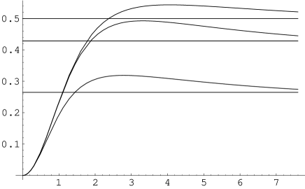
Figure 4: $2m/r$ versus $r$ for $\kappa=1,\ \frac{1}{3},\ \frac{1}{9}$ (highest: $\kappa=1$, lowest: $\kappa=\frac{1}{9}$) for the same conditions as previous Figures.

To obtain now a system with finite size we can imagine to enclose our fluid inside a perfectly insulating spherical cavity, with area radius $R$, and to assume that thermodynamical equilibrium is reached, that is the temperature of the walls is equal to the temperature of fluid at $r=R$. This will correspond to a certain central energy density $\rho_{C}$ for the cavity. Due to the local uniqueness of solutions to equation (19) with initial conditions (20), this is equivalent to take a certain (physical) solution to equation (19) (that with $\rho(0)=\rho_{C}$) and to cancel all fluid outside $r=R$. As regards energy density radial profile $\rho(r)$, this means that there is a 1-1 correspondence between all admitted cavities filled with linear fluids (that is every admitted central densities as well radii) and all possible $\rho(r)$ distributions in finite ranges [0,$R$], where $\rho(r)=1/(8\pi f^{g}(r))$ and $f$ is solution to (19) with initial conditions (20).

As allowed by Birkhoff theorem Wheeler ; Birkhoff , if the constraining system is assumed spherically symmetric and with finite extension, the Schwarzschild coordinates can be chosen in such a way that outside a certain radius $R^{*}$ exactly the Schwarzschild form of the metric obtains

$$ds^{2}=-(1-2M^{*}/r)\ dt^{2}+\frac{1}{1-2M^{*}/r}\ dr^{2}+r^{2}d\Omega^{2}.$$ (36)

The parameter $M^{*}$ here is precisely the mass-energy or ADM mass for the whole system, that is fluid + constraining system. Due to our symmetry conditions we can look at the quantity

$$M=\int_{0}^{R}{4\pi r^{2}\rho(r)dr}=\frac{C}{2}\int_{0}^{R}{\frac{r^{2}}{f^{g}(r)}dr},$$ (37)

as the mass due to the fluid alone, that is the mass would be probed by Kepler-like experiments with gravitating bodies far away from the fluid alone. It represents a meaningful quantity, proper of the ball of fluid contained in the cavity, independent of the characteristics (mass, extension,..) of the constraining system. As the metric outside has been explicitly chosen, the continuity of the metric tensor components $g_{\alpha\beta}$ everywhere, even across boundaries, fixes, for every assigned $\rho_{C}$ and $g$, $f(r)$ $\forall r$. Due to (15) the value of $C$ is fixed also. In other words, once a single coordinate system is explicitly chosen, the arbitrariness in the choice of the constant $C$ in equations (9)-(10) is lost.

Fig. 5 permits to see, for a cavity with fixed area radius $R$ at equilibrium, the dependence of its mass on the central density or temperature, for different assigned $g$. It reports $2M/R$ as a function of $z\equiv\rho(0)R^{2}$.

Figure 5: $2M/R$ versus $z\equiv\rho(0)R^{2}$ ($R$ can be thought fixed), for $\kappa=1,\ \frac{1}{3},\ \frac{1}{9}$ (highest: $\kappa=1$, lowest: $\kappa=\frac{1}{9}$).

The plot is done in terms of $z$ instead of $\rho(0)\equiv y$ in order to obtain for $2M/R$ an universal shape, i.e. not depending on the chosen $R$. The expression for $z$ indicates how to rescale the abscissa to obtain, from the given plot, the actual relation between $2M/R$ and $y$ for each fixed value of $R$. The explicit form of the plotted function, expressed in terms of the solution $h_{1}$ for initial conditions (26) (the solution $h$ presented in Fig. 2), is

$$\frac{2M(z)}{R}=\frac{h_{1}(\sqrt{8\pi z})-1}{h_{1}(\sqrt{8\pi z})}$$ (38)

as can be easily derived from equation (29) and from the scaling property (24). A maximum $(2M/R)_{max}=0.544$ is found (with the extremal point at $z_{extr}=0.655$), corresponding to the case $g=1$ ($\kappa=1$); it gives the maximum fraction of the Schwarzschild mass a perfect linear fluid at equilibrium confined inside a given radius can have. The maximum value for the case $g=2$ ($\kappa=1/3$), namely $(2M/R)_{max}=0.493$, is in agreement with sorkin . All these results agree with what reported in Chavanis , where in addition a prescription is given to relate $(2M/R)_{max}$ values when $\kappa$ is varied.

In Fig. 5 we see that once the extremal central energy density or temperature are overcome, equilibrium configurations are still possible, at lower values of $M$. We have thus larger central temperatures, which give rise however to a lower total mass for the system. This is by no way a problem for energy conservation, obviously. The total energy of the system, given by $M$, contains in fact both the component of proper energy $\rho$ and the (negative) component of gravitational potential energy Wheeler ; misner_sharp . Evidently, when the extremal temperature is overcome, the system admits a new equilibrium configuration with a stronger gravitational energy component.

A detailed discussion of the stability of the confined fluids we are considering here is in Chavanis . According to those results a new mode on instability occurs whenever a (non trivial) local extremum in our Fig. 5 is present. This amounts to say that, as far the equilibrium of the fluid alone is considered (neglecting the constraining system katz ), starting from a situation of stability at low $z$ (very low energy density and/or very small radius), the first maximum marks the transition to instability and this latter will never desappear for larger values of $z$, so that stability is for $z\leq z_{extr}$. This agrees with the results in sorkin corresponding to the case $\kappa=\frac{1}{3}$ and with the general discussion of thermodynamic equilibrium and stability conditions in katz2 .

III Non-extensivity

The aim of this section is to characterize the systems under study in terms of their degree of non-extensivity. This is done using the methods introduced in Oppen2 , generalizing them to the case of gravitating systems subject to an external pressure.

The first law of thermodynamics as applied to an infinitesimal volume $dV$ of a homogeneus system reads

$$dE=T\ dS-p\ dV+\mu\ dN,$$ (39)

where $dE$, $dS$ and $dN$ are respectively energy, entropy and number of particles in the volume $dV$, and $\mu$ the chemical potential. Integrating this equation to a tiny volume $V$ means to sum over elementary volumes, each possessing always the same values of the intensive quantities. If the quantities on which we integrate are extensive, that is if they scale with size, integration gives

$$E=TS-pV+\mu N,$$ (40)

so that this relation (known as Gibbs-Duhem relation) requires and manifests extensivity. This can conveniently be expressed as $1=\frac{TS}{E}$ or $1=\frac{TS}{E+pV}$ or $1=\frac{TS}{E+pV-\mu N}$ if, respectively, no $p$ and $\mu$ terms, $p$ terms or $p$ and $\mu$ terms are chosen to be included in the expression of $S$. In particular, without $p$ and $\mu$ terms in $S$, a linear relation

$$S(\lambda E)=\lambda S(E)$$ (41)

is implied, where the variations of $E$ and $S$ are intended with intensive quantities fixed. This is certainly the case of most thermodynamic systems also at macroscopic level (our systems included), when the volume $V$ is the whole volume of the system at thermodynamic equilibrium, provided gravitational interaction or, in general, long range interactions can be neglected (as often assumed, at least implicitly, in thermodynamics) Oppen2 . In this case the intensive quantities are intended to have values $T_{0}$, $p_{0}$ and $\mu_{0}$ characterizing globally the system.

When however gravitational effects become no longer negligible one can expect that relation (40), albeit holding true locally (equivalence principle), be modified at a global level (with a suitable definition of the intensive quantities for this case), revealing thus non-extensivity. Correspondingly, relation (41) should be modified to

$$S(\lambda M)=\lambda^{a}\ S(M),$$ (42)

where $a$ is a constant $\neq 1$ and we have indicated with $M$ the total energy of the system. Entropy is no longer extensive with energy, but related to it by an Euler relation of homogeneity $a\neq 1$.

Looking at the analogy between the properties of local temperature in a lattice model with long range spin-spin interactions and the local temperature behaviour for gravitating systems as given by Tolman relation, the suggestion has been made in Oppen2 to define a global temperature $T_{0}$ for gravitating systems, to be identified with the temperature $T_{\infty}$ that would be measured by an observer far away (in an asymptotically flat spacetime). Given this definition, thermodynamic consistency demands that for gravitating systems in self-equilibrium, or, in general, for closed systems not influenced mechanically by any external agent, the equation

$$S=\alpha\frac{M}{T_{0}}$$ (43)

be an Euler relation of homogeneity $1/\alpha$ in $M$, provided $S$ here is intended as total entropy deprived of its component dependent on $\mu$ (if present). In fact the first law (39) implies $1/T_{0}=\partial{S}/\partial{M}$. In other terms, putting $\gamma\equiv 1/a$, we obtain $\gamma=\alpha$ or

$$\gamma=\frac{T_{0}S}{M},$$ (44)

so that any $\gamma\neq 1$ signals and measures non-extensivity.

Black holes obey this relation, as can be verified through the explicit expressions of black hole temperature and entropy or, more directly, through the Smarr relation smarr

$$S=\frac{M}{2T_{0}}$$ (45)

(see Oppen2 ; Oppen1 ) where we see $\gamma=1/2$, so that correspondingly $S(M)\propto M^{2}$.

Analogously (and intriguingly) for any classical gravitating system in self-equilibrium, approaching its own Schwarzschild radius, (conventional) entropy satisfies this same relation (45) giving thus again $\gamma=1/2$ Oppen1 . In Oppen2 , equation (44) has been applied to a gravitating system in self-equilibrium consisting of a perfect fluid at constant density and the variation of $\gamma$ with $M/R$ (being $R$ the radius of the system) has been investigated.

Attempting to extend the above analysis to our case, we face here the problem that, contrary to the cited cases, our systems are constrained to be in the assigned volume by an external pressure $p_{ext}$ applied at $r=R$, so that they cannot be considered mechanically insulated. Applying however the same reasoning that leads to equations (43-44), we see that these equations still hold true also in case an external pressure is present, provided $S$ is intended as total entropy deprived now also of the component due to a $p_{ext}\neq 0$. That is we have

$$\gamma=\frac{T_{0}S_{0}}{M},$$ (46)

where with $S_{0}$ we intend the component of $S$ obtained assuming $p_{ext}=0$ (in addition to $\mu=0$).

Let us now evaluate total entropy for our systems. The Gibbs-Duhem relation (40), as applied locally, expressed in specific form

$$\rho=Ts-p+\mu n$$ (47)

gives

$$s=\frac{1}{T}\ (\rho+p-\mu n).$$ (48)

From this, considering that to deprive $s$ of the component of $p$ due to the presence of a $p_{ext}\neq 0$ means to quit the whole $p$ (i.e. $p_{ext}=0$ implies $p=0$, for the fluids under study if, as at present, they are constrained to be in a finite volume), we have

$$S_{0}(y)=\int_{0}^{R}4\pi r^{2}\frac{\rho}{T}\sqrt{h}\ dr=b^{1/2g}\int_{0}^{R}4\pi r^{2}\left(\frac{1}{8\pi}\right)^{\frac{2g-1}{2g}}\left(\frac{1}{f(r)}\right)^{\frac{2g-1}{2}}\sqrt{h(r)}\ dr$$

where $y=\rho(0)$ and $f$, $h$ are determined by this initial condition with $C=1$ (and with assigned $g$) and use of equations (6-8) is made, with (6) in the form

$$\rho=b\ T^{2g},$$ (49)

with $b$ a constant. We further obtain

$$S_{0}(y)=b^{\frac{1}{2g}}y^{\frac{2g-1}{2g}}4\pi\int_{0}^{R}r^{2}\left(\frac{1}{f_{1}(\sqrt{8\pi y}\ r)}\right)^{\frac{2g-1}{2}}h_{1}(\sqrt{8\pi y}\ r)^{1/2}\ dr,$$ (50)

where the expression for $S_{0}(y)$ depends only on the solutions for the initial conditions $f(0)=1$; here use of the equation

$$f(r)=\frac{1}{(8\pi y)^{1/g}}f_{1}(\sqrt{8\pi y}\ r)$$ (51)

is made, relation that can readily be obtained from scaling property (23). Expressing the integration in (50) in terms of the variable ${\tilde{z}}\equiv yr^{2}$ we finally obtain

$$S_{0}(z)=b^{\frac{1}{2g}}y^{-\frac{1}{2g}-\frac{1}{2}}2\pi\int_{0}^{z}\sqrt{\tilde{z}}\left(\frac{1}{f_{1}(\sqrt{8\pi{\tilde{z}}})}\right)^{\frac{2g-1}{2}}h_{1}(\sqrt{8\pi{\tilde{z}}})^{1/2}\ d{\tilde{z}},$$ (52)

where $z=y\ R^{2}$ (as in (38)).

From equation (48) we see that $s$ is given by three components, each in principle with its own radial profile. For our systems however these radial profiles are the same. In fact from equations (6) and (7), we see that $s$, $\rho/T$ and $p/T$ terms depend only on $T$, with a same dependence, so that the same must hold for the $\mu n/T$ term also. This assures the $\mu n/T$ term, if present, has the same radial profile as the $\rho/T$ term. Total entropy with all the components included, is then proportional to $S_{0}$ so that the two entropies have a same scaling law with $M$.

As regards global temperature $T_{0}$, from Tolman relation (5) and from (49) and (8) we have

$$T_{0}=T_{C}\sqrt{f(0)}=b^{-1/2g}(8\pi)^{-1/2g}C^{1/2g},$$ (53)

where, as said, $T_{0}$ is the temperature measured by a far away observer. We see that $T_{0}$ is sensitive to the value of $C$, that on its own should depend on the mass-energy distribution of the whole system, constraining system included. Global temperature however is, like energy $M$ or entropy $S$, a thermodynamical parameter that, as such, must be characteristic of the chosen system it describes, irrespective of its environment. Moreover, if the constraining system is, as we suppose, in thermal equilibrium with the fluid contained in it, a same far away temperature $T_{0}$ must coherently be measured, independently of the characteristics (density, size, ..) of the constraining system. From (53) this implies that, once the asymptotic flatness of the metric is required, the actual value of $C$ is fixed, irrespectively of the characteristics of the constraining system. We are thus led to compute $T_{0}$ as the far away temperature evaluated as if the constraining system would be absent. From the continuity of the metric tensor component on the boundary of the cavity we have then

$$f(R)=1-2M/R,$$ (54)

so that from (8)

$$\frac{C}{(1-2M/R)^{g}}=\frac{1}{f(R)^{g}},$$ (55)

where, as above, $f$ is the solution with $C=1$ and $y=\rho(0)$. From this equation and from (38) and (51) we obtain the following expression for $C$

$$C=8\pi y\ \frac{1}{[h_{1}(\sqrt{8\pi z})f_{1}(\sqrt{8\pi z})]^{g}},$$ (56)

so that $T_{0}$ is

$$T_{0}=b^{-\frac{1}{2g}}y^{\frac{1}{2g}}\ \frac{1}{[h_{1}(\sqrt{8\pi z})f_{1}(\sqrt{8\pi z})]^{1/2}}.$$ (57)

From this expression for $T_{0}$ and from the expression (52) for entropy $S$, $\gamma$ as given by (46) can finally be written. Noting that $M$, given by equation (38), can also be written as

$$M=2\pi y^{-\frac{1}{2}}\ \int_{0}^{z}\sqrt{\tilde{z}}f_{1}(\sqrt{8\pi{\tilde{z}}})^{-g}\ d{\tilde{z}}$$

(from (37), once the integration variable is changed from $r$ to ${\tilde{z}}=y\ r^{2}$), for $\gamma$ the expression

$$\gamma(z)=\frac{T_{0}S_{0}}{M}=[h_{1}(\sqrt{8\pi z})f_{1}(\sqrt{8\pi z})]^{-1/2}\cdot\frac{\int_{0}^{z}\sqrt{\tilde{z}}f_{1}(\sqrt{8\pi{\tilde{z}}})^{-g}[h_{1}(\sqrt{8\pi{\tilde{z}}})f_{1}(\sqrt{8\pi{\tilde{z}}})]^{1/2}\ d{\tilde{z}}}{\int_{0}^{z}\sqrt{\tilde{z}}f_{1}(\sqrt{8\pi{\tilde{z}}})^{-g}\ d{\tilde{z}}}$$ (58)

is found.

IV Scaling laws and radial profiles

Fig.6 plots $\gamma(z)$ as given by equation (58).

Figure 6: $\gamma$ versus $z\equiv\rho(0)R^{2}$ for $\kappa=1,\ \frac{1}{3},\ \frac{1}{9}$ (highest: $\kappa=\frac{1}{9}$, lowest: $\kappa=1$).

At each $z$ value, we have $S(M)\propto M^{1/\gamma}$ with $\gamma$ given by the plot. We see that in the limit $z\rightarrow 0$ (low densities and/or small radii), $\gamma\rightarrow 1$, so that $S(M)\propto M$ (and $S(R)\propto R^{3}$, from (37)) and extensivity obtains. This can analytically be seen from (58), as in this limit from (26) and (16) we have $f,h\simeq 1$ and $\gamma$ reduces to

$$\gamma(z)\simeq\frac{\int_{0}^{z}\sqrt{\tilde{z}}\ d{\tilde{z}}}{\int_{0}^{z}\sqrt{\tilde{z}}\ d{\tilde{z}}}=1.$$ (59)

In the limit $z\rightarrow\infty$ (very high densities and/or large radii), from (32) and (33) we get

$$\gamma(z)\simeq z^{-\frac{1}{2g}}\cdot\frac{\int_{0}^{z}\sqrt{\tilde{z}}\ {\tilde{z}}^{-1+\frac{1}{2g}}\ d{\tilde{z}}}{\int_{0}^{z}\sqrt{\tilde{z}}\ {\tilde{z}}^{-1}\ d{\tilde{z}}}=\frac{\frac{1}{2}}{\frac{1}{2g}+\frac{1}{2}}=\frac{g}{g+1},$$

so that asymptotically $\gamma(z)=\frac{1}{2},\ \frac{2}{3},\ \frac{5}{6}$ respectively for $g=1,\ 2,\ 5$ ($\kappa=1,\ \frac{1}{3},\ \frac{1}{9}$). In this limit thus $S(M)\propto M^{2}$ for $g=1$ and $S(M)\propto M^{\beta}$ with $1<\beta<2$ for $g>1$. Due to (31) or (38) this means also $S(R)\propto R^{2}$ for $g=1$ and $S(R)\propto R^{\beta}$ for $g>1$. Note that this limit can be achieved at any fixed $R$, if central energy density $y$ is allowed to increase to sufficiently large values, and we remain far from the Schwarzschild mass limit.

The graph of $\gamma$ intersects the asymptote at each extremal point of $\frac{2M}{R}$ of equation (38) (or of Fig.5). From our discussion about the stability of equilibrium configurations, this implies that the $z$ region of stability has both $d\gamma/dz\leq 0$ and $\gamma(z)$ above its asymptote. The intersections with the asymptote also mean that for each configuration corresponding to a local maximum of $\frac{2M}{R}$, the asymptotic behaviour of $S(M)$ is locally recovered; for the $g=1$ case this in particular implies that $S(M)\propto M^{2}$ for each such finite $z$. This means that equilibrium configurations exist (stable, in the case of the first maximum), with $y$ and $R$ both finite, with exact $S(M)\propto M^{2}$ (and, due to extremality, $S(R)\propto R^{2}$) local scaling.

Fig.7 illustrates this.

Figure 7: $S/M^{2}$ (arbitrary units) versus $z$ for $\kappa=1$.

We see that for $z=z_{extr}=0.655$ (the first extremal point, see Fig.5), $S/M^{2}$ has a local extremum, implying $S/M^{2}\simeq const$ there. At the same time this (in addition to (59)) verifies the definition of $\gamma$ as given by (46).

These results confirm and, in some respects, extend what found for these systems in banks . Within the stability interval in $z$, $\gamma$ decreases at increasing $M/R$, as said, and this is somehow analogous to the result obtained in Oppen2 , in the study of the relation between $\gamma$ and $M/R$ for a self-gravitating system consisting of a perfect fluid at constant density. The behaviour of conventional entropy $S(R)\propto R^{2}$ confirms the statement that no horizon is needed to have an entropy that scales like the area Oppen2 ,Oppen1 ; as our systems are far from the Schwarzschild limit (even when $z\rightarrow\infty$) this statement is confirmed in a strong sense: to have an area scaling entropy, not even the approaching to horizon formation is required banks .

In terms of global temperature $T_{0}$, one can show that, in the limit $z\rightarrow\infty$, our systems have $T_{0}\propto 1/R$ banks , in addition to the area scaling law for entropy, so that the analogy with black hole thermodynamics is quite complete. This happens also for self-gravitating systems near to reach their own Schwarzschild radius Oppen1 . To see the $T_{0}$ dependence on $R$, with reference to equation (57) we write $T_{0}R$ as

$$T_{0}R=b^{-\frac{1}{2g}}y^{\frac{1}{2g}-\frac{1}{2}}\frac{z^{1/2}}{[h_{1}(\sqrt{8\pi z})f_{1}(\sqrt{8\pi z})]^{1/2}}\equiv\eta(y)\xi(z)$$ (60)

and in Fig.8 we plot $\xi(z)$ for $g=1,\ 2,\ 5$ (highest: $g=5$, lowest: $g=1$), together with the constant value asymptotically approached by $\xi(z)$ in the $g=1$ case revealing the $1/R$ law for $T_{0}$.

Figure 8: $\xi$ (representing $T_{0}R$, see text) versus $z$ for $\kappa=1,\ \frac{1}{3},\ \frac{1}{9}$ (highest: $\kappa=\frac{1}{9}$, lowest: $\kappa=1$).

From (60), together with equations (32) and (33), the asymptotic behaviour of $T_{0}R$ can analytically be inferred. We have $T_{0}R\propto z^{0},\ z^{1/4},\ z^{2/5}$ (corresponding to $T_{0}R\propto R^{0},\ R^{1/2},\ R^{4/5}$) respectively for $g=1,\ 2,\ 5$ and the asymptote in Fig.8 is at $\frac{1}{2\sqrt{8\pi}}$.

For the $g=1$ case note that every time $z$ is extremal (for $2M/R$), that happens every time the $\xi(z)$ curve intersects the asymptote in Fig.8, the slope is not 0 and thus $T_{0}R$ does not scale as $1/R$ there, not even locally, notwithstanding the area scaling law for entropy. This is expected, as $T_{0}(z)=\frac{1}{dS_{0}/dM}$ and $S_{0}(M)\propto M^{1/\gamma(z(M))}$, so that, near each extremal $z$, the $1/R$ law can set in only if $\gamma(z)\simeq const$ there, that is when $z\rightarrow\infty$. We have thus that only in the limit $z\rightarrow\infty$ the thermodynamic analogy among the systems of present study and the black holes and the classical systems of Oppen1 extends to both $S$ and $T_{0}$ scaling laws.

Let us consider now the radial profiles of entropy. We are mainly interested in their relation with the strength of the gravitational interaction, as given by the parameter $M/R$, and in the shape they take when area scaling law for entropy obtains, in particular in the limiting case $z\rightarrow\infty$ in which the $1/R$ scaling law for temperature also applies. From

$$S=\int_{0}^{R}4\pi r^{2}s(r)\sqrt{h}\ dr=\int_{0}^{R}4\pi r^{2}\sigma(r)\ dr,$$ (61)

in addition to the entropy local density $s$, an entropy “radial” density $\sigma$ is defined (in order to compare with Oppen2 ). As already discussed, the three components of $s$ as given in (48) have the same radial profiles. We can then restrict the study of entropy radial profiles to the component $s=\rho/T$ alone. From (49) and (51) we have

$$s(r)=b^{1/2g}\rho(r)^{\frac{2g-1}{2g}}=b^{1/2g}y^{\frac{2g-1}{2g}}f_{1}(\sqrt{8\pi y}\ r)^{-g+\frac{1}{2}}=b^{1/2g}y^{\frac{2g-1}{2g}}f_{1}(\sqrt{8\pi z}\ x)^{-g+\frac{1}{2}}\equiv\chi(y)\psi_{z}(x),$$ (62)

$$\sigma(r)=b^{1/2g}y^{\frac{2g-1}{2g}}f_{1}(\sqrt{8\pi z}\ x)^{-g+\frac{1}{2}}h_{1}(\sqrt{8\pi z}\ x)^{\frac{1}{2}}\equiv\chi(y)\omega_{z}(x),$$ (63)

where $x\equiv\frac{r}{R}$ covers the interval [0,1] and $\omega_{z}(x)=\psi_{z}(x)h_{1}(\sqrt{8\pi z}\ x)^{\frac{1}{2}}$. Being $f_{1}$ monotonically increasing, we expect $\psi_{z}(x)$ to be monotonically decreasing, becoming steeper with growing $z$.

For the $g=1$ case, the most interesting one as regards entropy scaling laws, Figures 9 and 10 report respectively $\psi_{z}(x)$ and $\omega_{z}(x)$, for $z=0,\ \frac{z_{extr}}{2},\ z_{extr}=0.655$, where $z_{extr}$ is the first extremal point, corresponding to the higher edge of the stability interval in $z$. The straight line corresponds to $z=0$, while the lowest curve corresponds to $z=z_{extr}$.

Figure 9: Entropy local density $s$, normalized to its value at the centre $s(0)$, versus radius (normalized to 1) for different $z$ values (different $M/R$ values), $z=0,\frac{z_{extr}}{2},z_{extr}$. The straight line is for $z=0$ ($M/R=0$); the steepest curve is for $z=z_{extr}$ ($M/R$ is at its maximum).

Figure 10: Entropy “radial” density $\sigma$ (see text), normalized to its value at the centre $\sigma(0)$), versus radius (normalized to 1) for the same $z$ values as the previous Figure. Straight line: $z=0$; lowest curve: $z=z_{extr}$.

From Fig.5 (or relation (38)) we recall that $M/R$ increases with $z$, from 0 at $z=0$, up to its maximum allowed value for $z=z_{extr}$. $s(r)$ or $\sigma(r)$ profiles become thus flat as the strength of gravitational interaction is negligible, as expected, while they become decreasing with $r$ when $M/R\neq 0$, being increasingly steeper with $M/R$ growing. We have thus that the weight of the internal regions in the determination of total entropy grows with $M/R$. This can be seen also in Fig.11, where the quantity $x^{2}\psi_{z}(x)$ is reported ($\propto 4\pi r^{2}s(r)dr$, the entropy on the slice at radius $r$).

Figure 11: $r^{2}s$ ($\propto$ entropy of the slice at radius $r$) versus $r$ with $s$ normalized to its value at the centre $s(0)$ and $r$ normalized to 1, for the same $z$ values as previous Figures. Uppermost curve: $z=0$; lowest curve: $z=z_{extr}$.

The uppermost curve corresponds to $z=0$, while the lowest one to $z=z_{extr}$. The weight of external slices is progressively decreasing when $M/R$ grows from $M/R=0$ (case with the expected quadratic dependence on $r$ of the entropy of slices of that radius) to its maximum value. The behaviour of our system is at variance in this respect with the self-gravitating system consisting of a perfect fluid with constant density, studied in Oppen2 . In that case the weight of external layers is shown to increase with $M/R$, as reported by Fig.2 of Oppen2 , the equivalent of our Fig.10.

For $z>z_{extr}$ the curves for $s(r)$ and $\sigma(r)$ become increasingly steeper and it is interesting to explore what is the shape the radial profiles acquire in the limit $z\rightarrow\infty$; as we know in fact in this limit for the case $g=1$ we have both the area scaling law for entropy and the $1/R$ law for temperature. For $z\rightarrow\infty$, from (62) and (33) we find

$$\psi_{z}(x)\simeq\left[\left(\frac{2m}{r}\right)_{\infty}^{-\frac{1}{g}}(8\pi z)^{\frac{1}{g}}x^{\frac{2}{g}}\right]^{-g+\frac{1}{2}}\propto x^{-2+\frac{1}{g}}$$ (64)

and from (32) a same behaviour for $\omega_{z}(x)$. This means that in this limit $s(r)$ and $\sigma(r)$ behave like $1/r$ if $g=1$ and like $1/r^{\delta}$ with $1<\delta<2$ for any other allowed $g$; in the limit $g\rightarrow\infty$ (dust), $\delta=2$. We see thus that for our systems, when we are at conditions in which both the area scaling for entropy and the $1/R$ law for temperature set in, the entropy radial profile goes as $1/r$, with a larger weight from internal layers in the determination of total entropy, as compared to the no-gravity case. This is at variance with what happens for self-gravitating classical systems that reach the above scaling laws for entropy and temperature while approaching their Schwarzschild radius, for which it is demonstrated that in this limit all entropy lies on the surface Oppen1 .

V Conclusions

In conclusion we have seen that the area scaling law for entropy as well the $1/R$ law for temperature (the celebrated properties of black hole thermodynamics) can set in also for classical finite systems even at circumstances very far from the formation of an horizon. We have shown moreover that when this happens, entropy radial profile may be completely different from what found for the systems that gain the above scaling laws while approaching horizon formation, in which case entropy lies on their surface Oppen1 .

We have studied the onset of these properties for systems consisting of perfect fluids with linear equation of state $p=\kappa\rho$, constrained in a finite volume by an external pressure. The above properties set in at limiting conditions of causality banks ($\kappa=1$) and size/energy density ($R$ and/or $\rho\rightarrow\infty$), being however safely far from horizon formation limit. These results have been obtained generalizing the methods introduced in Oppen2 for the study of non-extensivity of thermodynamical parameters in gravitating systems, to the case in which an external pressure is applied. The entropy radial profile we find in the limiting circumstances in which the mentioned scaling laws for entropy and temperature set in is $s(r)\propto 1/r$, so that a heavy contribution is given by the internal layers, contrary to what happens for the systems Oppen1 . This is thus a case in which the whole volume contributes to the total number of degrees of freedom of the system (with a heavier specific contribution from internal regions), being however this number scaling like the area.

References

- (1) J. Oppenheim, Phys. Rev. E68 (2003) 016108, gr-qc/0212066.
- (2) S. Hawking, Comm. Math. Phys. 43 (1975) 199.
- (3) J. Bekenstein, Lett. Nuovo Cimento 4 (1972) 737.
- (4) G. ’t Hooft, “ Dimensional reduction in quantum gravity”, essay dedicated to Abdus Salam, published in Salamfest (1993) 0284, gr-qc/9310026.
- (5) L. Susskind, J. Math. Phys. 36 (1995) 6377, hep-th/9409089.
- (6) T. Banks, W. Fischler, A. Kashani-Poor, R. McNees and S. Paban, Class. Quant. Grav. 19 (2002) 4717, hep-th/0206096.
- (7) Ya. B. Zel’dovich, Zh. Eksperim. i Teor. Fiz. 41 (1961) 1609, Soviet Phys.-JETP 14 (1962) 1143.
- (8) R. Bousso, Rev. Mod. Phys. 74 (2002) 825, hep-th/0203101, and references therein.
- (9) J. Oppenheim, Phys. Rev. D65 (2002) 024020, gr-qc/0105101.
- (10) C. Tsallis, Chaos Solitons Fractals 13 (2002) 371, and references therein.
- (11) A. Renyi, in Proc. of 4th Berkeley Symposium on Mathematical Statistics and Probability, Vol.1 (1961) 547.
- (12) C.W. Misner, K.S. Thorne and J.A. Wheeler, Gravitation, W.H. Freeman and Company, New York, 1973.
- (13) S. Chandrasekhar, “A limiting case of relativistic equilibrium”, in General Relativity, papers in honour of J.L. Synge, ed. by L. O’Raifeartaigh (Clarendon, Oxford) (1972) 185.
- (14) R.C. Tolman, Phys. Rev. 55 (1939) 364.
- (15) J.R. Oppenheimer and G.M. Volkoff, Phys. Rev. 55 (1939) 374.
- (16) R.C. Tolman and P. Ehrenfest, Phys. Rev. 36 (1930) 1791.
- (17) T. Banks and W. Fischler, hep-th/0111142.
- (18) T. Banks and W. Fischler, hep-th/0102077.
- (19) H.-J. Schmidt and F. Homann, Gen. Rel. Grav. 32 (2000) 919, gr-qc/9903044.
- (20) R.D. Sorkin, R.M. Wald and Z. Zhen Jiu, Gen. Rel. Grav. 13 (1981) 1127.
- (21) H. Bondi, Proc. R. Soc. London, Ser. A, 282 (1964) 303.
- (22) P.H. Chavanis, Astron. Astrophys. 381 (2002) 709, astro-ph/0108230.
- (23) C.W. Misner and H.S. Zapolsky, Phys. Rev. Lett. 12 (1964) 635.
- (24) G. D. Birkhoff, Relativity and Modern Physics, Harvard University Press, Mass., 1923.
- (25) C.W. Misner and D.H. Sharp, Phys. Rev. 136 (1964) B571.
- (26) J. Katz and Y. Okuta, Class. Quant. Grav. 12 (1995) 2275, gr-qc/9409021.
- (27) J. Katz, Found. Phys. 33 (2003) 223, astro-ph/0212295.
- (28) L. Smarr, Phys. Rev. Lett. 30 (1973) 71.