Cosmology as a search
for overall equilibrium

Abstract

In this letter we will revise the steps followed by A. Einstein when he first wrote on cosmology from the point of view of the general theory of relativity. We will argue that his insightful line of thought leading to the introduction of the cosmological constant in the equations of motion has only one weakness: The constancy of the cosmological term, or what is the same, its independence of the matter content of the universe. Eliminating this feature, I will propose what I see as a simple and reasonable modification of the cosmological equations of motion. The solutions of the new cosmological equations give place to a cosmological model that tries to approach the Einstein static solution. This model shows very appealing features in terms of fitting current observations.

PACS: 04.20.Gz, 04.62.+v, 04.70.-s, 04.70.Dy, 04.80.Cc
Keywords: cosmological models, vacuum energy, Einstein Universe

1 Introduction

The way Einstein arrived at his formulation of a cosmological model for the universe was based on two basic hypothesis [1]. From the one side, he was struggling with the idea that a single particle in the Universe couldn’t have inertia as inertia should have a relational origin. From the other side, he thought that the universe could be described as a gas of stars close to equilibrium. After some intricate reflections, he arrived to the notion of a finite universe without boundary, and static on the overall, that is, at equilibrium. For that he introduced the now famous cosmological constant as a way of compensating the purely-attractive behaviour of matter in his equations.

In 1930 A. Eddington proved that Einstein’s static Universe was unstable under homogeneous departures from the equilibrium state [2]. This together with the observation of the recession of galaxies led progressively to the abandonment of Einstein model. Anyway, the Einstein model has been the subject of several investigations over the years [see for example [3]-[6]]. The most recent is a revision of its possible role as the initial state for a past eternal universe [7].

Our point of view in this letter is that the reasoning that led Einstein to his model is too powerful to be simply abandoned. Of course, from nowadays perspective, his assumption of a universe at precise overall equilibrium clearly needs some revision. But more importantly, one needs to revise his way of incorporating an equilibrating mechanism by adding a cosmological constant.

At that time, physicist didn’t seem to suspect that the cosmological term could be just another type of manifestation of matter, what we now use to call a vacuum-energy contribution. For example, now we know that the presence of any quantum field in nature could give place naturally to a vacuum-energy contribution with an equation of state of the form $p_{V}=-\rho_{V}$. However, when the quantum fields are considered as fundamental, the naive calculation of this vacuum-energy contribution is always huge, being completely at odds with the observations (apart from being completely independent of the total amount of energy in the non-vacuum component of the field).

In recent years we have learnt, mostly through the works of G. Volovik [10, 11], that the universe that we experience might be an emergent structure “living” at the low-energy corner of a fundamental quantum system with a finite number of degrees of freedom, similar somehow to a quantum liquid. Remarkably, in these systems the set of excitations with respect to the vacuum state include collective-excitations, describable in terms of geometrical (gravitational) an electromagnetic fields, and quasi-particle excitations, describable as quantum matter (fermionic) fields. A very interesting insight coming out from the observation of these systems is that, the calculation of a vacuum energy contribution performed by adding the zero-point energies associated to the quantization of the different quasi-particles modes leads to grossly incorrect results. Vacuum-energy has to be calculated by other means.

It is not difficult to understand that for a condensed matter system to have an equilibrium vacuum state in the absence of external forces its vacuum pressure has to vanish, $p_{V}=0$ . This is exactly what happen with quantum liquids. Now, if these type of systems are brought out of their lowest energy state by exciting, for example, a thermal cloud of quasi-particles within them, they tend to reach a new state of internal equilibrium. The pressure associated with the quasi-particles, $p_{M}$, is equilibrated by a newly generated vacuum term $p_{V}$ such that $p_{M}+p_{V}=0$. In this way we see that the vacuum term is not constant, but depends on the characteristics of the matter contribution, tending to counterbalancing it. The exact counterbalance occurs only at precise equilibrium. If these systems were set up out of equilibrium, they would evolve towards the equilibrium point. During this transient regime one would have $p_{M}+p_{V}\neq 0$.

Another line of thought, this time exclusively within the context of gravitational interactions, that also suggest the existence of an equilibrating mechanism is the following. Einstein gravitational law, expressed as $G_{\mu\nu}=8\pi GT_{\mu\nu}^{M}$, has been seen to work to a high degree of accuracy in the astronomical (as opposed to cosmological) context (in the weak field limit they precisely give place to Poisson’s equation $\nabla^{2}\phi=\rho_{M}$ for the Newtonian potential $\phi$). However, if the universe was on the overall a three sphere (finite without boundary), one would expect in Newtonian terms that a quantity of localized matter will affect another quantity of localized matter with two direct contributions, associated with the shortest and the longest geodesic path between the two masses, plus additional contributions associated with geodesic paths connecting them after having traverse entirely the universe one or several times. Some of these contributions are attractive (as the one associated with the shortest direct path between the masses) but some other are effectively repulsive (as the one associated with the longest direct path). As a result, two masses at a fixed distance will affect each other differently depending on the size of the universe. For example, in a extreme situation, two masses located at antipodal points of a closed universe would exert no net-force into each other. We can symbolically write the global result of all these gravitational interactions as a modified Poisson equation

$$\nabla^{2}\phi=\rho_{I}(\phi,\rho_{M})\;,$$ (1.1)

where $\rho_{I}$ identifies an effective matter source depending on the real matter density but also on the geometry of the universe itself (here represented only by the scalar potential). Thinking in this way, it is not difficult to reach the conclusion (as Einstein did) that Einstein equations should be modified to deal with cosmological situations. These modified equations should contain cosmological solutions (homogeneous and isotropic) that are static. The easiest modification one can think of that do the job is one in which the global effects of matter are separated into a normal contribution and a cosmological contribution equilibrating each other – this is precisely Einstein universe. However, there is no reason to adopt the much stronger assumption that the cosmological term is constant.

The possible existence of a varying cosmological term was considered as early as in 1933 by M. Bronstein [12] (see for example [13] and [14] for reviews of the history of the cosmological term). Nowadays there are many models incorporating a varying cosmological term (mainly under the names of quintessence [15] and dark energy [16]; see also [13, 14] and references therein for a summary of different models). Generically, the idea has been that since inflation (or some other phase transitions in the early universe) the contribution of an effective cosmological term has been progressively disappearing, leaving a small or zero contribution at present. The cosmological contribution has been usually modelled as an independent field. Here we are going to treat the cosmological contribution as completely tied up with the normal matter content.

In the following we will propose a simple heuristic modification of the cosmological equations of motion incorporating an equilibrating, and so variable, cosmological term. Adjustment mechanisms have been explored before (see [17] for an updated discussion). The difference here is that instead of describing a specific and detailed adjusting mechanism an see what happens, we take as an starting hypothesis the very existence of an equilibrating mechanism. The equations that we propose to implement this mechanism are arguable the simplest one can think of, and are enough to illustrate the main features of these type of models.

2 The model

Let us assume that it exists a state of stable internal (by definition there is nothing outside the Universe) equilibrium for the universe on the overall . To describe the situation let us separate the total effect of matter on the geometry as a normal contribution and a so-called vacuum contribution. For concreteness and simplicity let us choose an equation of state for matter of the form $p_{M}=(\gamma-1)\rho_{M}$ with $\gamma\in(4/3,1)$. The equation of state for the vacuum energy is $p_{V}=-\rho_{V}$.

The Friedman equation for a universe with closed spherical spacial sections is

$$\left({\dot{a}\over a}\right)^{2}=-{1\over a^{2}}+{8\pi G\over 3}\rho_{T}\;,$$ (2.1)

where $\rho_{T}$ contains the matter density and the vacuum energy contribution: $\rho_{T}=\rho_{M}+\rho_{V}$. The equation for the acceleration of the scale factor is

$${\ddot{a}\over a}=-{4\pi G\over 3}(\rho_{T}+3p_{T})\;.$$ (2.2)

The Einstein static universe is obtained when

$$(\rho_{T}+3p_{T})=0\;,~{}~{}~{}~{}~{}~{}{8\pi G\over 3}\;a^{2}\rho_{T}=1\;$$ (2.3)

and $a=a_{s}$ equal constant. In this case

$$\rho_{V}={3\gamma-2\over 2}\rho_{M}~{}~{}~{}{\rm and}~{}~{}~{}a_{s}^{-2}={8\pi G\over 3}{3\gamma\over 2}\rho_{M}\;.$$ (2.4)

Now let us eliminate the condition $\rho_{V}:=$constant. This condition is obtained if one requires that the conservation of the energy-momentum tensor applies separately to the normal-matter and vacuum-energy components. When this is not the case, from the total conservation equation

$${d\rho_{T}\over da}=-{3\over a}(\rho_{T}+p_{T})\;,$$ (2.5)

one obtains

$${d\rho_{V}\over da}=-\left({d\rho_{M}\over da}+{3\gamma\over a}\rho_{M}\right)\;.$$ (2.6)

This equation and Friedman’s equation have to be supplemented with a third equation to obtain a closed set of equations. The third equation will be the one that regulates the transference of energy between the normal and the vacuum energy components. A simple choice one can make is

$${d\over da}\left[\rho_{V}-{(3\gamma-2)\over 2}\rho_{M}\right]=-{1\over\tau}\;\rho_{V}\;.$$ (2.7)

We will show that this nicely incorporates the idea that the universe has the tendency to go towards the equilibrium point. The constant parameter $\tau$ can be interpreted as a relaxation time and sets the strength of the tendency towards the equilibrium: As smaller is $\tau$ the greater is this tendency. At this stage, we don’t have a fundamental theory from which to calculate the value of $\tau$, we just take it as a parameter of the model.

Let us now first solve equations (2.6) and (2.7). The general solution will be expressed in terms of two arbitrary constants $C_{1}$ and $C_{2}$. Once found the functions $\rho_{V}=\rho_{V}(a,C_{1},C_{2})$ and $\rho_{M}=\rho_{M}(a,C_{1},C_{2})$ we can plague them into the Friedman equation to solve for the scale factor. Friedman’s equation, (2.1), can be written as

$${1\over 2}\dot{a}^{2}+V_{\rm Newt-eff}(a)=0\;,$$ (2.8)

with

$$V_{\rm New-eff}(a)\equiv{1\over 2}\left\{1-{8\pi G\over 3}a^{2}[\rho_{V}(a)+\rho_{M}(a)]\right\}\;.$$ (2.9)

In this form it is very easy to extract its physical information.

So, from equations (2.6) and (2.7) we obtain a second order equation for $\rho_{M}$:

$${d^{2}\rho_{M}\over da^{2}}+\left({2\over a}+{2\over 3\gamma}{1\over\tau}\right){d\rho_{M}\over da}+\left({2\over a\tau}-{2\over a^{2}}\right)\rho_{M}.$$ (2.10)

The general solution of this second order differential equation is

$$\rho_{M}(a)= C_{1}a^{-1}\exp\left(-{1\over 3\gamma}{a\over\tau}\right)\;M_{3\gamma-1,3/2}\left({2\over 3\gamma}{a\over\tau}\right)$$ (2.11)

$$+C_{2}a^{-1}\exp\left(-{1\over 3\gamma}{a\over\tau}\right)\;W_{3\gamma-1,3/2}\left({2\over 3\gamma}{a\over\tau}\right)\;,$$

where $M_{\kappa,\lambda}$ and $W_{\kappa,\lambda}$ identify Whittaker’s functions [18]. Now one can also solve for $\rho_{V}(a)$:

$$\rho_{V}={3\gamma\over 2}\;\tau\;{d\rho_{M}\over da}+3\gamma\;{\tau\over a}\;\rho_{M}\;.$$ (2.12)

A remarkable fact to notice is that although there are two independent solutions to previous equation, only $M_{3\gamma-1,3/2}$ is different from zero for $a>0$. Therefore concerning the behaviour of the different magnitudes for positive $a$, only the value of $C_{1}$ is relevant.

In figure 1 we have plotted a generic behaviour of $\rho_{V}(a)$, $\rho_{M}(a)$ and $V_{\rm New-eff}(a)$. We have chosen $C_{1}=100$, $C_{2}=0$, $\gamma=1.25$, $\tau=100$ and $8\pi G/3=0.0002$ for graphical clarity.

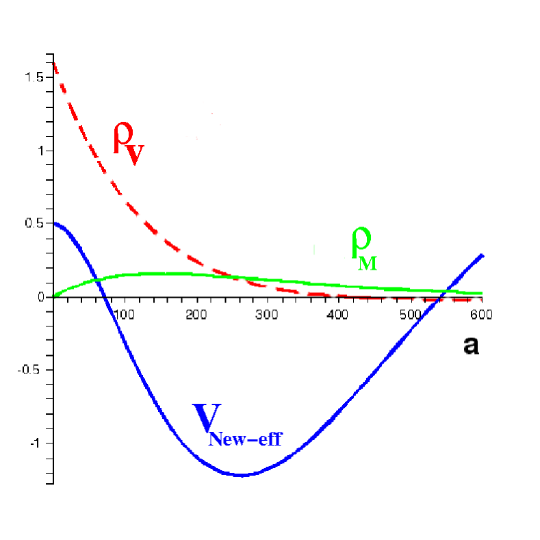
Figure 1: Plots of $\rho_{V}(a)$, $\rho_{M}(a)$ and $V_{\rm Newt-eff}(a)$ showing a generic solution of our set of cosmological equations. We have used $\gamma=1.25$ $C_{1}=100$, $C_{2}=0$, $\tau=100$ and $8\pi G/3=0.0002$ for graphical clarity.

The red dashed line, the green bold line and the blue bold line represent $\rho_{V}$, $\rho_{M}$ and $V_{\rm New-eff}$ respectively. We clearly observe that the previous set of equations give place generically to oscillating universes between a minimum and a maximum size [remember that the Newtonian effective energy is equal zero; see (2.8)]. The Einstein solution is a fine-tuned solution corresponding to the situation in which the bottom of the potential is precisely at the zero-energy level. However, within this framework Einstein’s solution would be stable. The generic cosmological solutions found are such that at a large value of the vacuum energy density the universe is small but not singular; at that point the matter energy density is small. Then, as the universe expands, the vacuum energy density rapidly decreases while the matter energy density increases. In this process the matter energy density becomes sufficiently large so that, at some maximum size, the system stops its expansion being driven to re-collapse towards the original point. Then, the cycle is repeated over and over. Oscillating models caused by a cosmological term diminishing with the expansion have been consider before in [20]. In that paper instead of introducing as here an equation of transference of energy, they analyse different functional forms for the dependence of $\rho_{V}$ with the scale factor.

The model has only two adjustable parameters: The time relaxation parameter $\tau$ and the initial value of $\rho_{M}$. The initial value of $\rho_{V}$ is then also fixed. This reflects the fact that we are really not dealing with two matter sources but with a single one effectively described as separated into two terms.

3 Cosmological observations

The presented oscillating universe only considers the homogeneous and isotropic degree of freedom of the gravitational and matter sectors. In a more realistic setting, the energy on the homogeneous and isotropic mode would decrease owing to the transfer of energy to inhomogeneous modes. Then, one can define an entropic birth for the universe as the starting point of a cycle at which all of the inhomogeneous modes were unexcited. In terms of the cosmological time, the universe has not a beginning; instead the universe is past eternal. Therefore, if one takes any snapshot in the evolution having some inhomogeneities present and, then, evolve backwards in time, one will always find a cosmological time in the past at which all the inhomogeneous modes were unexcited. This “initial” cycle would have the largest amplitude (that is, the largest difference between $a_{\rm min}$ and $a_{\rm max}$). Then, each new cycle would have a smaller amplitude than the previous. Eventually, the homogeneous mode of the universe would settle down at the Einstein equilibrium point.

The validity of a cosmological model can only be assessed by the observations. Thus, this model will have to surpass several tests in the future. At this stage I can only say that it has very appealing features including its falsifiability:

• It is reasonable to think that we are already leaving in a world of low-energies (all the phenomena around us happen at energy scales much lower that Planck scale). It is also reasonable to think that we are neither almost at the equilibrium point (in the cosmological sense) nor close to the initial state. In terms of entropy, there is already bast amounts of entropy in the universe, but clearly, we are very far from a maximal entropy state. Therefore, starting from this observation our model tell us that the values of $\rho_{M}$ and $\rho_{V}$ should be of the same order. This so-called coincidence is something that we observe and has been part of the motivation for the present analysis.

• Taking the currently accepted values of $\Omega_{\Lambda}\sim 0.7$ and $\Omega_{M}\sim 0.3$ [21], our model predicts that the acceleration that we observe should be decreasing with time at present and so be bigger in the past. The fitting of the supernova data at high redshifts seems to provide an indication of the contrary [22]. The acceleration appears as nonexistent in the past, giving support to models of dark energy as the Chaplygin gas (see for example [23]). However, by making global comparisons between different cosmological models, other authors argue that it is still impossible to discern, for example, between a cosmological constant and varying dark energy [24].

  Another prediction of this model is that the normal-matter energy density at present and at the recent past would have to have a different evolution that in standard cosmological models. For a dust dominated universe ($\gamma=1$) one only has to compare the standard and modified behaviours:

  $${d\rho_{M}\over da}=-{3\over a}\;\rho_{M}~{}~{}~{}~{}{\rm versus}~{}~{}~{}~{}{d\rho_{M}\over da}=-{2\over a}\;\rho_{M}+{2\over 3\gamma}\;{1\over\tau}\;\rho_{V}\;.$$ (3.1)

• The “close to Big Bang” origin of the universe in our model allows for incorporating most of the predictive power of this paradigm. However one has to bear in mind that any realistic calculation within our model will have to take into account two new factors: i) Since its entropic birth, the universe could have passed through a few entire cycles before entering in its current expansive phase; ii) In each new cycle, the maximum value of the acceleration attained, proportional to $\rho_{V}-[(3\gamma-2)/2]\rho_{M}$, would be smaller.

  For example, the diminishing of the duration of a single phase of nucleosynthesis, owing to the background acceleration predicted for that period, could be compensated with the plausible existence of a few cycles reaching large enough temperatures for nuclear reactions to take place.

• In this model the time elapsed since the entropic birth of the universe (Big Bang-like) would be much larger than in standard cosmological models. We have much more time to produce structures in the universe, something that has always been problematic in standard cosmology.

• This model does not have the so-called horizon problem of standard cosmology as there is not a “beginning of time” event. Therefore, radiation could have enough time to thermalize in very large scales. If the current cycle would have started at a temperature smaller than $T_{\rm recombination}$, then, the size of the inhomogeneities found in the cosmic microwave radiation would not directly constraint the size of the inhomogeneities in the barionic matter sector in recent times.

• Within this positive curvature model, the found values $\Omega_{\Lambda}+\Omega_{M}\sim 1$ and $H_{0}^{-1}\sim 14.000$ Gyears would be just telling us that the universe is very large, $R_{0}\geq 100$ Gpc with $R_{0}$ its current physical radius, so locally it would be almost flat.

Further checking of the compatibility of this cosmological model with actual observations will be the subject of future work.

References

- [1] A. Einstein, Sitzungsberichte der Königlich Preussischen Akademie der Wissenschaften 142, (1917); Also in a translated version in The principle of Relativity, (Dover, New York, 1952).
- [2] A. S. Eddington, Mon. Not. Roy. Astron. Soc. 90, 668 (1930).
- [3] G. Lemaître, Mon. Not. Roy. Astron. Soc. 91, 490 (1931).
- [4] W. B. Bonnor, Mon. Not. Roy. Astron. Soc. 115, 310 (1954).
- [5] E. R. Harrison, Rev. Mod. Phys. 39, 862 (1967).
- [6] G. W. Gibbons, Nucl. Phys. B 292, 784 (1987).
- [7] J. D. Barrow, G. F. R. Ellis, R. Maartens and C. G. Tsagas, Class. Quant. Grav. 20, L155 (2003) [arXiv:gr-qc/0302094].
- [8] W. Nerst, Verh. Dtsch. Phys. Ges. 18, 83 (1916)
- [9] Ya. B. Zel’dovich, Zh. Eksp. Teor. Fiz., Pis’ma Red. 6, 883 (1967) [JETP Lett. 6, 316 (1967)].
- [10] G. E. Volovik, “The Universe in a Helium Droplet,” (Clarendon Press, Oxford, UK, 2003).
-
[11]
G. E. Volovik,
“Vacuum energy: Myths and reality,”
arXiv:gr-qc/0604062;
Annalen Phys. 14, 165 (2005). [arXiv:gr-qc/0405012]. - [12] M. Bronstein, Phys. Z. Sowjetunion 3, 73 (1933).
- [13] P. J. E. Peebles and B. Ratra, Rev. Mod. Phys. 75, 559 (2003) [arXiv:astro-ph/0207347].
- [14] T. Padmanabhan, Phys. Rept. 380, 235 (2003) [arXiv:hep-th/0212290].
- [15] R. R. Caldwell, R. Davé and P. J. Steinhardt, Phys. Rev. Lett. 80, 1582 (1998).
- [16] M. S. Turner, in The Galactic Halo, Astronomical Society of the Pacific Conference Proceedings No. 165, edited by B. K. Gibson, T. S. Axelrod, and M. E. Putnam (Astronomical Society of the Pacific, San Francisco 1999).
- [17] A. D. Dolgov, Int. J. Mod. Phys. A 20, 2403 (2005).
- [18] M. Abramowicz and I. A. Stegun, Handbook of Mathematical Functions (Dover, New York, 1972)
- [19] C. Barceló and G. Volovik, JETP Lett. 80, 209 (2004) [Pisma Zh. Eksp. Teor. Fiz. 80, 239 (2004)] [arXiv:gr-qc/0405105].
- [20] J. M. Overduin and F. I. Cooperstock, Phys. Rev. D 58, 043506 (1998) [arXiv:astro-ph/9805260].
- [21] D. N. Spergel et al. [WMAP Collaboration], Astrophys. J. Suppl. 148, 175 (2003) [arXiv:astro-ph/0302209].
- [22] A. G. Riess et al. [Supernova Search Team Collaboration], Astrophys. J. 607, 665 (2004) [arXiv:astro-ph/0402512].
- [23] O. Bertolami, A. A. Sen, S. Sen and P. T. Silva, Mon. Not. Roy. Astron. Soc. 353, 329 (2004) [arXiv:astro-ph/0402387].
- [24] A. R. Liddle, P. Mukherjee, D. Parkinson and Y. Wang, “Present and future evidence for evolving dark energy,” arXiv:astro-ph/0610126.