Light’s Bending Angle due to Black Holes: From the Photon Sphere to Infinity

Abstract

The bending angle of light is a central quantity in the theory of gravitational lensing. We develop an analytical perturbation framework for calculating the bending angle of light rays lensed by a Schwarzschild black hole. Using a perturbation parameter given in terms of the gravitational radius of the black hole and the light ray’s impact parameter, we determine an invariant series for the strong-deflection bending angle that extends beyond the standard logarithmic deflection term used in the literature. In the process, we discovered an improvement to the standard logarithmic deflection term. Our perturbation framework is also used to derive as a consistency check, the recently found weak deflection bending angle series. We also reformulate the latter series in terms of a more natural invariant perturbation parameter, one that smoothly transitions between the weak and strong deflection series. We then compare our invariant strong deflection bending-angle series with the numerically integrated exact formal bending angle expression, and find less than $1\%$ discrepancy for light rays as far out as twice the critical impact parameter. The paper concludes by showing that the strong and weak deflection bending angle series together provide an approximation that is within $1\%$ of the exact bending angle value for light rays traversing anywhere between the photon sphere and infinity.

I Introduction

One of the early striking predictions of General Relativity is that the weak-deflection bending angle of star light grazing the Sun is of the form

$${\hat{\alpha}}_{\rm Einstein}(r_{0})\,=\,4\,\left(\frac{{\sf m}_{\bullet}}{r_{0}}\right)\ +\ \mathcal{O}\left[{\left(\frac{{\sf m}_{\bullet}}{r_{0}}\right)}^{2}\right],\hskip 72.26999pt\mbox{\small\sf(First-Order Weak-Deflection)}$$ (1)

which at leading order is twice the value given by Newtonian gravity. Eddington’s 1919 confirmation of the leading term in (1) was the first observation of gravitational lensing and brought Einstein’s new gravitational theory instant scientific acclaim. Gravitational lensing in the weak-deflection limit has since been studied extensively, yielding numerous applications in astrophysics and cosmology (e.g., Schneider et al. 1992 sef , Petters et al . 2001 plw , Kochanek et al. 2005 ksw ). In addition, over the past two years weak-deflection lensing has been employed to create tests accessible to current or near-future instruments, of gravity theories such as PPN models and $5$-dimensional, string-theory inspired, braneworld gravity (Keeton and Petters 2005-2006 kp1 ; kp2 ; kp3 ). In kp1 , the first-order weak deflection formula (1) was also extended to all orders in ${\sf m}_{\bullet}/r_{0}$ and re-expressed as an invariant perturbation series (since $r_{0}$ is a coordinate dependent quantity coord-dep ). Interested readers may also find a recent analysis in DeLuca of the weak deflection limit.

In recent years, however, the exciting promise of planned space-borne black hole imaging instruments has ignited research activity in the analytical study of lensing in the strong-deflection regime (e.g, Virbhadra and Ellis 2000 ve , Frittelli, Kling, and Newman 2000 fkn , Eiroa, Romero, and Torres 2003 ert , Petters 2003 ptt , Perlick 2004 prk , Bozza, Capozziello, De Luca, Iovane, Mancini, Scarpetta, and Sereno 2001-2005 bozzaetal ).

For a Schwarzschild black hole of physical mass $M$, the spacetime geometry in the vicinity of the photon sphere at radius $r=3{\sf m}_{\bullet}$, where ${\sf m}_{\bullet}=GM/c^{2}$ is the black hole’s gravitational radius, is revealed through the resulting strong-deflection gravitational lensing. In 1959, Darwin darwin computed the first-order term of the bending angle of light traversing deep inside the black hole’s potential — i.e., close to the photon sphere:

$${\hat{\alpha}}_{\rm Darwin}(r_{0})\,=\,-\pi\ +\ 2\,\log\left[\frac{36(2-\sqrt{3})\,{\sf m}_{\bullet}}{r_{0}\,-\,3{\sf m}_{\bullet}}\right]\ +\ \mathcal{O}\left[{h^{\prime}}\right],\hskip 14.45377pt\mbox{\small\sf(First-Order Strong-Deflection)}$$ (2)

where $h^{\prime}=1-(3{\sf m}_{\bullet})/r_{0}$. He also showed analytically that near the photon sphere there are two families of relativistic images, which are images determined by light rays that loop around the photon sphere at least once before reaching the observer. Other authors have confirmed this strong-deflection multi-looping lensing effect (e.g., Atkinson 1965 atkinson , Luminet 1979 luminet , Chandrasekhar 1982 chandra , Ohanian 1987 ohanian , several recent authors ve -bozzaetal ). These studies were based on evaluating the lowest-order term (out from the photon sphere) of the light ray’s strong-deflection bending angle. Equation (2) is the well-known leading logarithmic deflection term.

In this paper, we develop a perturbative framework that allows us to generalize Darwin’s strong deflection result (2) to any order in $h^{\prime}$. Surprisingly, we also found that the leading logarithmic deflection term employed in the literature can be improved. Earlier studies (e.g., (darwin, , p. 188), (chandra, , p. 132)) arrived at the leading logarithmic expression by a perturbation scheme that seems to combine higher and lower order terms. (We leave a definite assessment to the judgment of the reader — see the Appendix.) By re-doing the perturbation theory and being careful to compare only terms of the same order, we obtain an improvement (i.e., more accurate expression) to the leading logarithmic deflection term. Furthermore, since $r_{0}$ is coordinate dependent coord-dep , we re-formulate our strong-deflection bending angle in terms of a coordinate-independent series. In particular, we compute this invariant series explicitly to $3$rd-order in the perturbation parameter $b^{\prime}=1-b_{c}/b$, where $b_{c}=3\sqrt{3}{\sf m}_{\bullet}$ is the critical impact parameter. Our perturbation framework was also used to compute the weak-deflection bending-angle series directly and we found it to be in complete agreement with the expansion found recently in kp1 . Finally, we show that our invariant bending-angle series is in excellent agreement with the numerically computed exact formal expression for the bending angle. This is done for both the strong and weak deflection limits, and the span from the photon sphere to infinity. These results should be applicable to analytical lensing studies across these regimes and serve as a limiting case to check bending angle results in spacetime geometries generalizing the Schwarzschild metric.

The outline of the paper is as follows: Section II expresses the light’s bending angle in a formal exact expression involving a difference of elliptic integrals of the first kind. In Section III, we expand the strong-deflection bending angle in terms of an invariant series going outward from the the photon sphere. This section includes the improvement to the logarithmic term. Finally, Section IV gives a numerical comparison between the perturbative and exact bending angles across the range from the photon sphere to infinity.

II Formal Exact Strong-Deflection Bending Angle

A Schwarzschild black hole is the unique static, spherically symmetric, asymptotically flat vacuum solution of the Einstein equation. The metric is given in Schwarzschild coordinates $(t,r,\theta,\phi)$ by

$${\rm d}s^{2}=-\left(1-\frac{2{\sf m}_{\bullet}}{\bar{r}}\right){\rm d}t^{2}\ +\ \left(1+\frac{2{\sf m}_{\bullet}}{\bar{r}}\right)^{-1}{\rm d}\bar{r}^{2}+\bar{r}^{2}\,(d\theta^{2}+\sin^{2}\theta\,d\phi^{2}),$$ (3)

where $t=c\tau$ and ${\sf m}_{\bullet}=GM/c^{2}$ (gravitational radius) with $\tau$ physical time and $M$ the physical mass of the black hole at the origin.

Consider a standard gravitational lensing situation where a point source and observer lie in the asymptotically flat region. In a typical lensing scenario, the source and observer are on opposite sides of the black hole. However, this restriction can be lifted in strong-deflection lensing. Suppose that the source is close to the optical axis passing through the observer and black hole. By spherical symmetry, it suffices to choose the source-to-observer light rays as lying in the equatorial plane ($\theta=\pi/2$). The Euler-Lagrange equations yield that the light rays are governed by (e.g., kp1 ):

$$\left(\frac{d\phi}{dr}\right)^{2}=\frac{1}{r^{4}\,\sqrt{1/b^{2}\ -\ (1\ -\ 2{\sf m}_{\bullet}/r)/r^{2}}},$$ (4)

where $b=|L/E|$ is the impact parameter with $L$ and $E$ the respective angular momentum and energy invariants of the light ray. Setting $u=1/r$, re-write (4) as

$$\left(\frac{du}{d\phi}\right)^{2} = u^{4}\left[\frac{E^{2}}{u^{4}L^{4}}-\frac{1}{u^{2}}\left(1-2{\sf m}_{\bullet}u\right)\right]$$ (5)

$$= 2{\sf m}_{\bullet}u^{3}-u^{2}+{1\over{b^{2}}}.$$

This cubic polynomial has a maximum of two positive roots and at most one negative root.

Writing (5) as

$$B(u)=2{\sf m}_{\bullet}(u-u_{1})(u-u_{2})(u-u_{3}),$$

we consider the case of one negative root $u_{1}$ and two distinct positive roots $u_{2}$ and $u_{3}$. The three roots, given in terms of an intermediate constant $Q$ that allows us to line up the roots in the order $u_{1}<u_{2}<u_{3}$ are given by (e.g., p. 130 chandra ):

$$u_{1}=\frac{r_{0}-2{\sf m}_{\bullet}-Q}{4{\sf m}_{\bullet}r_{0}},\quad u_{2}=\frac{1}{r_{0}},\quad u_{3}=\frac{r_{0}-2{\sf m}_{\bullet}+Q}{4{\sf m}_{\bullet}r_{0}}.$$

Here $r_{0}$ is the light ray’s distance of closest approach, which is determined from (e.g., Eq. (12) of kp1 ):

$$b^{2}=\frac{r_{0}^{3}}{r_{0}-2{\sf m}_{\bullet}}.$$ (6)

By comparing the coefficients in $B(u)$ to those in the original polynomial in equation(5), we obtain the following two relations between $Q$ and the quantities $b,{\sf m}_{\bullet},r_{0}$:

$$\frac{Q^{2}-{(r_{0}-2{\sf m}_{\bullet})}^{2}}{8{\sf m}_{\bullet}r_{0}^{3}}=\frac{1}{b^{2}},$$

which is equivalent to

$$Q^{2}=(r_{0}-2{\sf m}_{\bullet})(r_{0}+6{\sf m}_{\bullet}).$$

The bending angle of the lensed light ray is given by (e.g., Eq. (20) of kp1 ):

$$\hat{\alpha} = 2\int_{0}^{1/r_{0}}\frac{du}{\sqrt{2{\sf m}_{\bullet}(u-u_{1})(u-u_{2})(u-u_{3})}}-\pi$$

$$= \sqrt{\frac{2}{{\sf m}_{\bullet}}}\int_{0}^{1/r_{0}}\frac{du}{\sqrt{(u-u_{1})(u_{2}-u)(u_{3}-u)}}-\pi$$

Split the above integral into two parts to make the lower limit equal to the smallest root $u_{1}$:

$$\hat{\alpha}=\sqrt{\frac{2}{{\sf m}_{\bullet}}}\left[\int_{u_{1}}^{u_{2}}\frac{du}{\sqrt{(u-u_{1})(u_{2}-u)(u_{3}-u)}}\ -\ \int_{u_{1}}^{0}\frac{du}{\sqrt{(u-u_{1})(u_{2}-u)(u_{3}-u)}}\right]\ -\ \pi.$$ (7)

Now, the integrals in (7) can be realized as elliptic integrals of the first kind (see Byrd and Friedman byrd for an introduction to elliptic integrals):

$$\hat{\alpha}=\sqrt{\frac{2}{{\sf m}_{\bullet}}}\left[\,\frac{2\,F(\Psi_{1},k)}{\sqrt{u_{3}-u_{1}}}\ -\ \frac{2\,F(\Psi_{2},k)}{\sqrt{u_{3}-u_{1}}}\right]\ -\ \pi,$$

where $F(\Psi_{i},k)$ is an incomplete elliptic integral of the first kind with amplitudes

$$\Psi_{1}=\frac{\pi}{2},\quad\Psi_{2}=\sin^{-1}\sqrt{\frac{-u_{1}}{u_{2}-u_{1}}},$$

and modulus

$$k^{2}=\frac{u_{2}-u_{1}}{u_{3}-u_{1}}.$$

Explicitly,

$$\Psi_{2}=\sin^{-1}\sqrt{\frac{Q+2{\sf m}_{\bullet}-r_{0}}{Q+6{\sf m}_{\bullet}-r_{0}}},\quad k^{2}=\frac{Q-r_{0}+6{\sf m}_{\bullet}}{2Q}.$$

Hence, the exact bending angle simplifies to

$$\hat{\alpha}=4\sqrt{\frac{r_{0}}{Q}}\left[K(k)\ -\ F(\Psi,k)\right]\ -\ \pi,$$ (8)

where $K(k)$ and $F(\Psi,k)$ are the complete and incomplete elliptic integrals of the first kind, respectively, and $\Psi=\Psi_{2}$. As a check of (8), note that in the limit when ${\sf m}_{\bullet}\rightarrow 0$, we obtain $Q=r_{0}$, $k=0$ and $\Psi=\pi/4$, which in turn imply $K(k)=\pi/2$ and $F(\Psi,k)=\pi/4$ to give us zero deflection as expected.

It is important to add that the exact bending angle expression (8) serves mainly as a formal expression. The latter has to be evaluated to obtain explicit analytical and physical properties about the nature of the bending angle. Equations (1) due to Einstein and (2) due to Darwin are the first-order evaluations of (8) in the weak and strong deflection limits, respectively. The challenge of course is in evaluating (8) beyond those terms. The weak-deflection series in terms of the impact parameter out to many orders beyond (1) was found recently in kp1 . We shall now determine the strong-deflection series beyond (2), re-derive the weak series result in kp1 , and reformulate the weak series in terms of a new perturbation parameter to allow a seamless comparison covering the span from the strong to weak deflection limits — i.e., from the photon sphere to infinity.

III Expansion of Bending Angle Beyond the Photon Sphere

The photon sphere is defined by the radius $r=3{\sf m}_{\bullet}$, which marks an unstable photon orbit. Light rays that cross within the photon sphere are captured by the black hole (e.g., darwin ; chandra ). Using the relations given in Section II, we can see that exactly on the photon sphere the impact parameter invariant is given by the critical value $b_{c}=3\sqrt{3}{\sf m}_{\bullet}$. Photon orbits of interest to us are between $r_{0}=3{\sf m}_{\bullet}$ and $r_{0}=\infty$, and indeed our focus will be on the region closer to the photon sphere.

We first express $h^{\prime}$ in terms of $b^{\prime}$. Equation (6) is a cubic in $r_{0}$ that is readily solved to yield:

$$r_{0}=\frac{2\,b}{\sqrt{3}}\,\cos\left[\frac{1}{3}\,\cos^{-1}\left(\frac{-3\sqrt{3}\,{\sf m}_{\bullet}}{b}\right)\right].$$ (9)

The quantities $r_{0}$ and $b$ of course have very different physical meaning for the light rays. Relative to an inertial observer at infinity, the quantity $r_{0}$ is the distance of closest approach to the center of the black hole, while the impact parameter $b$ is the perpendicular distance from the black hole’s center to the asymptotic tangent line to the light ray converging at the observer. Overall, the quantity $r_{0}$ approaches $b$ as we extend into regions well beyond the photon sphere, but near the photon sphere, the values of $r_{0}$ and $b$ are different.

To seamlessly traverse from regions near the photon to those at infinity, a natural choice of invariant parameter is

$$b^{\prime}=1\ -\ \frac{b_{c}}{b},$$

which ranges from $0$ at the photon sphere to $1$ at infinity (asymptotically flat region).

III.1 Affine Perturbative Form for Bending Angle

Our goal is to show that the strong-deflection bending angle can be expressed as an “affine perturbation” series in $b^{\prime}$. More precisely, define an affine perturbation series about a function $g$ as

$$f(x)=(A_{0}+\cdots+A_{p}x^{p}+\cdots)\,g(x)\ +\ (B_{0}+\cdots+B_{q}x^{q}+\cdots),$$ (10)

where $A_{i}$ and $B_{i}$ are constants with $p$ and $q$ positive rational numbers. We shall demonstrate in Section III.4 that the bending angle has an invariant affine perturbation series of the form

$$\hat{\alpha}(b^{\prime}) = \Bigl{(}\sigma_{0}+\sigma_{1}\,(b^{\prime})+\sigma_{2}\,(b^{\prime})^{2}+\sigma_{3}\,(b^{\prime})^{3}+\cdots\,\Bigr{)}\,\log{\left(\frac{\lambda_{0}}{b^{\prime}}\right)}$$ (11)

$$\hskip 36.135pt\ +\ \Bigl{(}\rho_{0}+\rho_{1}\,(b^{\prime})+\rho_{2}\,(b^{\prime})^{2}+\rho_{3}\,(b^{\prime})^{3}+\cdots\,\Bigr{)},$$

where $\lambda_{0}$, $\sigma_{i}$ and $\rho_{i}$ are numerical constants. Note that (11) is not a Taylor series expansion because of the appearance of the logarithmic term. However, we shall see that this logarithmic term is not exactly (2).

III.2 Bending Angle Series Beyond the Logarithmic Term

We now consider the exact bending angle in the region around the photon sphere by expanding out from the photon sphere using $h={\sf m}_{\bullet}/r_{0}$. The expression for the bending angle can now be rewritten as a function of $h$ using the following useful relations:

$$Q = r_{0}\sqrt{(1-2h)(1+6h)}$$

$$k^{2} = \frac{\sqrt{(1-2h)(1+6h)}-(1-6h)}{2\sqrt{(1-2h)(1+6h)}}$$

$$\Psi = \sin^{-1}\sqrt{\frac{\sqrt{(1-2h)(1+6h)}-(1-2h)}{\sqrt{(1-2h)(1+6h)}-(1-6h)}}.$$

As $r_{0}$ increases from $3{\sf m}_{\bullet}$ to $\infty$, the parameter $h$ goes from $1/3$ to $0$, which corresponds to the invariant impact parameter increasing from $3\,\sqrt{3}{\sf m}_{\bullet}$ to $\infty$. Intuitively, when the bending angle is computed in the regime near $b=3\,\sqrt{3}{\sf m}_{\bullet}$, we speak of strong-deflection (since we shall show in Section III.2 that the bending angle can become arbitrarily large), while weak-deflection will refer to regions with large $b$.

Before proceeding with the substitution of the above quantities in the expression for bending angle, we present an example of the standard series expansions for a complete elliptic integral of the first kind (e.g., see page 298 in byrd ) in terms of the modulus $k$:

$$K(k)=\frac{\pi}{2}\left[1+\frac{1}{4}k^{2}+\frac{9}{64}k^{4}+\frac{25}{256}k^{6}+...\right]$$ (12)

or, in terms of the complementary modulus $k^{\prime}=\sqrt{1-k^{2}}$

$$K(k^{\prime})=\sum_{m=0}^{\infty}{{-1/2\atopwithdelims( )m}}^{2}\left[\ln\left(\frac{4}{k^{\prime}}\right)-b_{m}\right]k^{\prime 2m}$$ (13)

where $b_{0}=0$ and $b_{m}=b_{m-1}+\frac{2}{2m(2m-1)}$. These, along with other similar expansions for elliptic integrals, are used in the following: After re-expressing all quantities in terms of $h$, we use the above-mentioned series expansions for elliptic integrals to obtain an expression for the bending angle (8) in powers of $h$. Expanding around $h=0$ (region at infinity) yields

$$\hat{\alpha}(h)=4h + \left(-4+\frac{15}{4}\pi\right)h^{2}+\left(\frac{122}{3}-\frac{15}{2}\pi\right)h^{3}+\left(-130+\frac{3465}{64}\pi\right)h^{4}$$ (14)

$$+ \left(\frac{7783}{10}-\frac{3465}{16}\pi\right)h^{5}+\left(-\frac{21397}{6}+\frac{310695}{256}\pi\right)h^{6}+\mathcal{O}\left[{\left(h\right)^{7}}\right].$$

This is in exact agreement with the weak-deflection bending angle series found in kp1 .

To obtain the strong-deflection bending angle, we expand $\hat{\alpha}(h)$ out from the photon sphere $h=1/3$. It is then convenient to work in terms of $h^{\prime}=1-3h$. The coefficient $\sqrt{r_{0}/Q}$ of the bending angle (15) is given in terms of $h^{\prime}$ by

$$\sqrt{\frac{r_{0}}{Q}}=\left[\frac{3}{3+4(1-h^{\prime})h^{\prime}}\right]^{1/4}$$

while the modulus and amplitude are

$$k^{2}=\frac{\sqrt{3}-2\sqrt{3}h^{\prime}+\sqrt{3+4(1-h^{\prime})h^{\prime}}}{2\sqrt{3+4(1-h^{\prime})h^{\prime}}}$$

and

$$\Psi=\sin^{-1}\sqrt{\frac{3+6h^{\prime}-\sqrt{3}\sqrt{3+4(1-h^{\prime})h^{\prime}}}{12h^{\prime}}}.$$

Since the quantity

$$k^{\prime 2}\equiv 1-k^{2}=\frac{-\sqrt{3}+2\sqrt{3}h^{\prime}+\sqrt{3+4(1-h^{\prime})h^{\prime}}}{2\sqrt{3+4(1-h^{\prime})h^{\prime}}}$$

approaches zero as $h^{\prime}\rightarrow 0$, it is convenient to re-write (8) in terms of $k^{\prime}$:

$$\hat{\alpha}=4\sqrt{\frac{r_{0}}{Q}}\left[\,K(\sqrt{1-k^{\prime 2}})\ -\ F(\Psi,\sqrt{1-k^{\prime 2}})\,\right]\ -\ \pi.$$ (15)

An $h^{\prime}$-series expansion for the elliptic integrals in (15) can then be obtained by first expanding in terms of $k^{\prime 2}$ and then expanding in $h^{\prime}$.

Remark: It is important to point out that if you want Mathematica to compute the functions $K(\sqrt{1-k^{\prime 2}})$ and $F(\Psi,\sqrt{1-k^{\prime 2}})$ as given in our notation, then the commands are ${\rm EllipticK}[1-k^{\prime 2}]$ and ${\rm EllipticF}[\Psi,1-k^{\prime 2}]$, respectively. It is incorrect to use ${\rm EllipticK}[\sqrt{1-k^{\prime 2}}]$ and ${\rm EllipticF}[\Psi,\sqrt{1-k^{\prime 2}}]$ because Mathematica defines ${\rm EllipticF}[\Psi,{\sf m}]=\int_{0}^{\Psi}\,(1-{\sf m}\,\sin^{2}\theta)^{-1/2}\,d\theta$ and ${\rm EllipticK}[{\sf m}]={\rm EllipticF}[\pi/2,{\sf m}].$

The bending angle series for (15) in terms of $h^{\prime}$ is then

$$\hat{\alpha}+\pi = \Bigl{[}8\,\tanh^{-1}(\sqrt{2}-\sqrt{3})+\log(144)-2\log(h^{\prime})\Bigr{]}\ +\ \frac{2h^{\prime}}{3}$$

$$+\frac{1}{18}\Bigl{[}-35+6\,\sqrt{3}+60\,\tanh^{-1}(\sqrt{2}-\sqrt{3})+15\log(12)-15\log(h^{\prime})\Bigr{]}\,h^{\prime 2}$$

$$+\frac{1}{162}\Bigl{[}295-36\,\sqrt{3}-360\,\tanh^{-1}(\sqrt{2}-\sqrt{3})-90\log(12)+90\log(h^{\prime})\Bigr{]}\,h^{\prime 3}$$

$$+\frac{1}{5184}\Bigl{[}-19637+3420\,\sqrt{3}+27720\,\tanh^{-1}(\sqrt{2}-\sqrt{3})+6930\log(12)-6930\log(h^{\prime})\Bigr{]}\,h^{\prime 4}$$

$$+\frac{1}{38880}\Bigl{[}211679-34200\,\sqrt{3}-277200\,\tanh^{-1}(\sqrt{2}-\sqrt{3})-69300\,\log(12)\Bigr{.}$$

$$\hskip 289.07999pt\Bigl{.}-\ 69300\,\log(h^{\prime})\Bigr{]}\,h^{\prime 5}$$

$$+\ \frac{1}{559872}\Bigl{[}-5580415+989964\,\sqrt{3}+7456680\,\tanh^{-1}(\sqrt{2}-\sqrt{3})\Bigr{.}$$

$$\hskip 144.54pt\Bigl{.}+\ 1864170\,\log(12)-1864170\,\log(h^{\prime})\Bigr{]}\,h^{\prime 6}\ +\ \mathcal{O}\left[{(h^{\prime})^{7}}\right].$$

The series (III.2) can be simplified significantly using the following:

$$8\,\tanh^{-1}(\sqrt{2}-\sqrt{3})+\log(144)-2\log(h^{\prime}) = 2\log\left(\frac{12(2-\sqrt{3})}{h^{\prime}}\right)$$

$$60\,\tanh^{-1}(\sqrt{2}-\sqrt{3})+15\log(12)-15\log(h^{\prime}) = 15\log\left(\frac{12(2-\sqrt{3})}{h^{\prime}}\right)$$

$$360\,\tanh^{-1}(\sqrt{2}-\sqrt{3})+90\log(12)-90\log(h^{\prime}) = 90\,\log\left(\frac{12(2-\sqrt{3})}{h^{\prime}}\right)$$

$$27720\,\tanh^{-1}(\sqrt{2}-\sqrt{3})+6930\log(12)-6930\log(h^{\prime}) = 6930\,\,\log\left(\frac{12(2-\sqrt{3})}{h^{\prime}}\right),$$

where we made use of $\tanh^{-1}(\sqrt{2}-\sqrt{3})=\frac{1}{4}\,\log(2-\sqrt{3}).$ The bending angle series can now be expressed more simply as follows:

$$\hat{\alpha} = -\pi\ +\ 2\log{\left(\frac{12(2-\sqrt{3})}{h^{\prime}}\right)}+\frac{2h^{\prime}}{3}+\frac{1}{18}\left[6\sqrt{3}-35+15\log{\left(\frac{12(2-\sqrt{3})}{h^{\prime}}\right)}\right](h^{\prime})^{2}$$ (17)

$$+ \frac{1}{162}\left[295-36\sqrt{3}-90\log{\left(\frac{12(2-\sqrt{3})}{h^{\prime}}\right)}\right](h^{\prime})^{3}$$

$$+ \frac{1}{5184}\left[-19637+3420\sqrt{3}+6930\log{\left(\frac{12(2-\sqrt{3})}{h^{\prime}}\right)}\right](h^{\prime})^{4}+\ \mathcal{O}\left[{(h^{\prime})^{5}}\right].$$

We can extend this series arbitrarily far, but the expressions become cumbersome and there is no need to do so for our later invariant analysis. Observe that $\hat{\alpha}$ becomes arbitrarily large as $h^{\prime}\rightarrow 0$ due to the first logarithmic term (and since the other logarithms are dominated by the given powers of $h^{\prime}$). This is the reason for the terminology strong deflection for light rays passing near the photon sphere.

III.3 Comparison with Darwin’s Logarithmic Bending Angle

The lowest order $h^{\prime}$-term in (17) is given by

$$\frac{\hat{\alpha}+\pi}{2}\ =\ \log\left(\frac{12(2-\sqrt{3})}{h^{\prime}}\right)\ +\ \mathcal{O}\left[{h^{\prime}}\right]\ =\ \log\left({\frac{12(2-\sqrt{3})r_{0}}{r_{0}-3{\sf m}_{\bullet}}}\right)\ +\ \mathcal{O}\left[{h^{\prime}}\right].$$ (18)

At first glance the reader may think that this term is the well-known logarithmic term found by Darwin 1959 darwin and employed commonly in the literature (e.g., Eqs. (262) and (268) in (chandra, , p. 132)). However, Darwin’s result is actually

$$\frac{\hat{\alpha}_{\rm Darwin}+\pi}{2}=\log\left({\frac{36(2-\sqrt{3}){\sf m}_{\bullet}}{r_{0}-3{\sf m}_{\bullet}}}\right).$$ (19)

Equations (18) and (19) are not identical! If the quantity $r_{0}$ in the numerator of equation (18) were replaced by $3{\sf m}_{\bullet}$, we obtain Darwin’s result, but this is not a legitimate substitution since the denominator would become zero. However, in the limit where $r_{0}$ approaches the photon sphere’s radius $3{\sf m}_{\bullet}$, equations (18) and (19) would both become infinitely large and so will be close in value in that limit.

In Section IV, we shall show explicitly how (18) is a better approximation than (19). For the convenience of the reader, we review in detail in the Appendix how (19) is derived. Note that in the derivation of (18), we were careful throughout to compare only terms at the same order, which allowed us to read off the lowest order term directly from the series expansion.

III.4 Invariant Bending Angle to Third Order Beyond Logarithmic Term

The strong-deflection bending angle series (17) is coordinate dependent since it is given in terms of the distance $r_{0}$ of closest approach. We now determine the bending angle in terms of the invariant quantity

$$b^{\prime}=1-\frac{b_{\rm c}}{b},$$

where $b_{\rm c}$ (critical impact parameter) is given by $b_{\rm c}=3\sqrt{3}{\sf m}_{\bullet}$. The quantity ranges over $[0,1]$ since $b$ increases outwards from the photon sphere at $b=b_{\rm c}$ to infinity.

In the Appendix, we derive the Darwin term (19) and show that it is equivalent to the following — see equation (36):

$$\hat{\alpha}_{\rm Darwin}+\pi=\log\left[{\frac{216(7-4\sqrt{3})\,(1-b^{\prime})}{b^{\prime}}}\right].$$ (20)

To express out bending angle in terms of the invariant $b^{\prime}$, we first write $h^{\prime}$ in terms of $b^{\prime}$ using the relationship (9) to get

$$h^{\prime}=1-\frac{(1-b^{\prime})}{2}\,\sec\left(\frac{1}{3}\,\cos^{-1}[-(1-b^{\prime})]\right).$$ (21)

Series expanding (21) in terms of $b^{\prime}$ gives

$$h^{\prime} = \sqrt{\frac{2}{3}}\,(b^{\prime})^{1/2}\ +\ \frac{2}{9}\,b^{\prime}\ -\ \frac{7}{54\sqrt{6}}\,(b^{\prime})^{3/2}\ +\ \frac{5}{243}\,(b^{\prime})^{2}\ -\ \frac{91}{3888\sqrt{6}}\,(b^{\prime})^{5/2}$$ (22)

$$\ +\ \frac{32}{6561}\,(b^{\prime})^{3}\ -\ \frac{2717}{419904\sqrt{6}}\,(b^{\prime})^{7/2}\ +\ \frac{88}{59049}\,(b^{\prime})^{4}\ +\ \mathcal{O}\left[{(h^{\prime})^{9/2}}\right].$$

For the weak deflection bending angle series (14), note that it is in a non-invariant form. To obtain an invariant expression, convert to the parameter $b^{\prime}$ by using $h=(1-h^{\prime})/3$ and then employing the series for $h^{\prime}$ in (22). This yields

$$\hat{\alpha}(b^{\prime}) = \frac{4}{3\sqrt{3}}(1-b^{\prime})+\frac{5\pi}{36}{(1-b^{\prime})}^{2}+\frac{128}{243\sqrt{3}}{(1-b^{\prime})}^{3}$$ (23)

$$\ +\ \frac{385\pi}{5184}{(1-b^{\prime})}^{4}+\frac{3584}{10935\sqrt{3}}{(1-b^{\prime})}^{5}\ +\ \mathcal{O}\left[{(1-b^{\prime})^{6}}\right].$$

The first term is the Einstein term (1) given in terms of $b^{\prime}$ by

$$\hat{\alpha}_{\rm Einstein}(b^{\prime})=\frac{4(1-b^{\prime})}{3\sqrt{3}}.$$ (24)

Turning to our strong-deflection bending angle expansion, insert the series (22) into the $h^{\prime}$-series (17) for strong deflection. This will yield a series in terms of the invariant $b^{\prime}$:

$$\hat{\alpha}(b^{\prime}) = -\pi\ +\ \log\Bigl{[}\frac{216\,(7-4\sqrt{3})}{b^{\prime}}\Bigr{]}\ +\ \frac{-17+4\,\sqrt{3}+5\,\log\Bigl{[}\frac{216\,(7-4\sqrt{3})}{b^{\prime}}\Bigr{]}}{18}\ b^{\prime}$$ (25)

$$\ +\ \frac{-879+236\,\sqrt{3}+205\,\log\Bigl{[}\frac{216\,(7-4\sqrt{3})}{b^{\prime}}\Bigr{]}}{1296}\ (b^{\prime})^{2}$$

$$\frac{-321590+90588\,\sqrt{3}+68145\,\log\Bigl{[}\frac{216\,(7-4\sqrt{3})}{b^{\prime}}\Bigr{]}}{629856}\ (b^{\prime})^{3}\ \ +\ \ \mathcal{O}\left[{(b^{\prime})^{4}}\right].$$

The lowest order term

$$\hat{\alpha}_{\rm lowest\ order}+\pi\equiv\log\left[\frac{216\,(7-4\sqrt{3})}{b^{\prime}}\right]$$ (26)

is similar, but not identical, to the Darwin logarithmic term (20) since (26) takes into account the improvement to Darwin’s result. The other terms in the series have not appeared in the literature before. Although the series expansion of $h^{\prime}$ in (22) involves fractional powers of $b^{\prime}$, there are no fractional power terms in the bending angle.

As promised in Section III.1, we rewrite (25) as an affine perturbation series about the logarithm:

$$\hat{\alpha}(b^{\prime}) = \Bigl{(}\sigma_{0}+\sigma_{1}b^{\prime}+\sigma_{2}(b^{\prime})^{2}+\sigma_{3}(b^{\prime})^{3}+\cdots\,\Bigr{)}\,\log\left(\frac{\lambda_{0}}{b^{\prime}}\right)$$ (27)

$$\hskip 72.26999pt+\Bigl{(}\rho_{0}+\rho_{1}b^{\prime}+\rho_{2}(b^{\prime})^{2}+\rho_{3}(b^{\prime})^{3}+\cdots\,\Bigr{)},$$

where $\lambda_{0}=216(7-4\sqrt{3})$ and the $\sigma$’s and $\rho$’s are constants given by

$$\sigma_{0} = 1\;\;\;\;\;\;\;\;\;\;\;\;\;\;\;\;\;\;\;\;\;\;\;\;{\rho_{0}}=-\pi$$

$$\sigma_{1} = \frac{5}{18}\;\;\;\;\;\;\;\;\;\;\;\;\;\;\;\;\;\;\;\;\;{\rho_{1}}=\frac{-17+4\sqrt{3}}{18}$$

$$\sigma_{2} = \frac{205}{1296}\;\;\;\;\;\;\;\;\;\;\;\;\;\;\;\;\;\;{\rho_{2}}=\frac{-879+236\sqrt{3}}{1296}$$

$$\sigma_{3} = \frac{68145}{629856}\;\;\;\;\;\;\;\;\;\;\;\;\;\;\;{\rho_{3}}=\frac{-321590+90588\sqrt{3}}{629856}.$$

The terminologies below will be employed for the terms of the affine series (27):

$$\mbox{$0$th-order:}\quad\sigma_{0}\,\log\left(\lambda_{0}/b^{\prime}\right)+\rho_{0}$$

$$\mbox{$1$st-order:}\quad\left(\sigma_{0}+\sigma_{1}b^{\prime}\,\right)\,\log\left(\lambda_{0}/b^{\prime}\right)\ +\ \left(\rho_{0}+\rho_{1}b^{\prime}\right)$$

$$\mbox{$2$nd-order:}\quad\left(\sigma_{0}+\sigma_{1}b^{\prime}+\sigma_{2}(b^{\prime})^{2}\,\right)\,\log\left(\lambda_{0}/b^{\prime}\right)\ +\ \left(\rho_{0}+\rho_{1}b^{\prime}+\rho_{2}(b^{\prime})^{2}\,\right)$$

$$\mbox{$3$rd-order:}\quad\left(\sigma_{0}+\sigma_{1}b^{\prime}+\sigma_{2}(b^{\prime})^{2}+\sigma_{3}(b^{\prime})^{3}\right)\,\log\left(\lambda_{0}/b^{\prime}\right)\ +\ \left(\rho_{0}+\rho_{1}b^{\prime}+\rho_{2}(b^{\prime})^{2}+\rho_{3}(b^{\prime})^{3}\right).$$

We have chosen to truncate at $3$rd-order because this order will already probe accurately as far as to twice the critical impact parameter. These issues are taken up in the next section.

IV Comparison of Perturbative and Exact Bending Angles

This section will give a numerical comparison of the formal exact bending angle with the zeroth, $1$st-, $2$nd- and $3$rd-order affine corrections to the logarithmic term. The comparison will be given by the following percentage discrepancy: $\displaystyle\left(\frac{\hat{\alpha}_{\rm exact}-\hat{\alpha}}{\hat{\alpha}_{\rm exact}}\right)\times 100\,\%.$

Figure 1: Percentage Discrepancy between Darwin’s logarithmic term, our $0$th-order logarithmic term, and the exact numerical value represented by the horizonatal axis. Our $0$th-order term is a better approximation to the exact value.

In Figure 1 is plotted the percentage discrepancy between the Darwin term (20) written in terms of $b^{\prime}$, our $0$th-order term (18), and the exact numerical value (8), which is represented by the horizontal axis. The $0$th-order term is closer to the exact value and comes within $1\%$ of the exact value at $b^{\prime}\approx 0.03$. The deviations increase for larger values of $b^{\prime}$.

If we include terms through to $3$rd-order in the strong deflection expression (27), then unlike the case in Figure 1, the series comes to within $1\%$ of the exact value for regions well past $b^{\prime}\approx 0.03$. Figure 2 shows that the regions could be as far out as to roughly twice the critical impact parameter (i.e., $b\approx 2b_{\rm c}$ or $b^{\prime}\approx 0.4705$) and still be within a $1\%$ discrepancy. Beyond this point the discrepancy continues to increase and will not be shown.

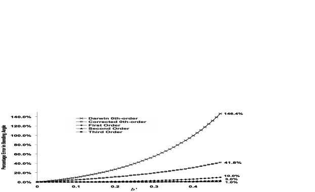
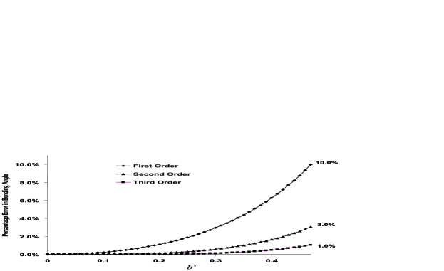
Figure 2: Top graph: Percentage discrepancy between the $0$th- to $3$rd-order terms, the Darwin logarithmic term, and the exact result given by the horizontal axis. The $3$rd-order result deviates by at most $1\%$ from the exact value with the maximum deviation at $b^{\prime}\approx 0.4705$. Bottom graph: A close-up of the same graph is plotted to show clearly the higher order corrections in more detail.

For the $5$th-order weak deflection bending angle series (23) and the Einstein term (24), Figure 3 shows the percentage discrepancies until (23) reaches a $1\%$ deviation. This occurs at $b^{\prime}\approx 0.4705$ and has a larger deviation for greater $b^{\prime}$ values.

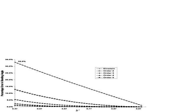
Figure 3: Percentage discrepancy corresponding to various orders of the weak deflection bending angle. The horizontal axis corresponds to the exact value. The $5$th-order expansion has a $1\%$ discrepancy at $b^{\prime}\approx 0.04705$.

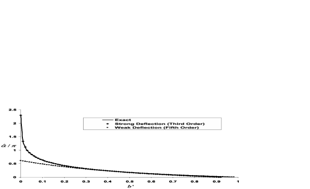
Figure 4: The 3rd-order strong deflection and the 5th-order weak deflection are plotted alongside the numerically integrated exact formal bending angle.

Figure 4 shows both the $3$rd-order strong deflection (27) and $5$th-order weak deflection (23) plotted alongside the exact result. The same comparison, in terms of the percentage discrepancy is presented in Figure 5. This graph illustrates that if (27) is used on the interval $0<b^{\prime}\lesssim 0.4705$ and (23) on the interval $0.4705\lesssim b^{\prime}<1$, then together these two series deviate by at most $1\%$ from the exact value. In addition, the $1\%$ maximum deviation occurs at $b^{\prime}\approx 0.4705$. These two series can then yield bending angle information rather accurately from the photon sphere to infinity.

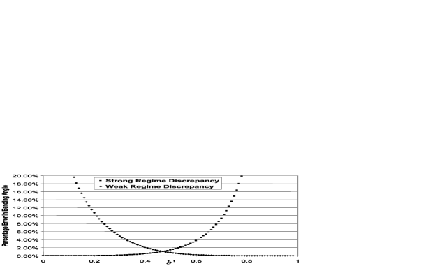
Figure 5: Percentage discrepancy for $3$rd-order strong deflection and $5$th-order weak deflection. The horizontal axis corresponds to the exact value. The two discrepancies criss-cross essentially at $1\%$ for $b^{\prime}\approx 0.4705$.

V Conclusions

An analytical perturbation framework for calculating the bending angle of light rays traversing the gravitational field of a Schwarzschild black hole was given. We expressed the strong-deflection bending angle in an invariant affine perturbation series in $b^{\prime}$ about a logarithmic function. Our logarithmic expression was shown to be a better approximation to the exact bending angle than the logarithmic one found by Darwin, which is commonly used in the literature. We also derived the known weak deflection bending angle series as a consistency check of our framework. The latter series was reformulated in terms of the more natural perturbation parameter $b$, which smoothly transitions from strong deflection near the photon sphere to weak deflection at infinity. Comparison was then given of our invariant strong deflection bending-angle series with the numerically integrated exact formal bending angle expression. We found less than $1\%$ discrepancy for light rays as far out as twice the critical impact parameter. This was followed by a further comparison with our invariant form of the weak deflection series. It was found that taken together, the two series yield an approximation that is within $1\%$ of the exact bending angle value for light rays traversing anywhere between the photon sphere and infinity.

Appendix A Derivation of the Darwin Term

For the convenience of the reader, we present here the standard bending angle derivation as in (chandra, , p. 132). The formal exact bending angle $\alpha$ is given (8) by

$$\frac{1}{2}(\pi+\hat{\alpha})=2\left(\frac{r_{0}}{Q}\right)^{1/2}\left[K(k)-F(\Psi,k)\right],$$

where

$$Q=\sqrt{(r_{0}-2{\sf m}_{\bullet})(r_{0}+6{\sf m}_{\bullet})},\quad k^{2}=\frac{Q-r_{0}+6{\sf m}_{\bullet}}{2Q},\quad\Psi=\sin^{-1}\sqrt{\frac{Q+2{\sf m}_{\bullet}-r_{0}}{Q+6{\sf m}_{\bullet}-r_{0}}}.$$

For the reader’s convenience, the correspondence between our notation and that in (chandra, , p. 132) is as follows: $(\pi+\hat{\alpha})/2=\phi_{\infty}$, $\hat{\alpha}=\Theta$, $P=r_{0}$, $D=b$, and $D_{c}=b_{c}$.

The perturbation scheme in (chandra, , p.132) is defined by setting

$$r_{0}={\sf m}_{\bullet}(3+\delta).$$ (28)

Note that $\delta$ does not remain under the value $1$ as one moves away from the photon sphere. The value of $\delta$ is assumed to be small compared to $3$. This is important for the approximations to follow. Series expanding and keeping terms at $1$st-order in $\delta$ yields

$$Q=\sqrt{(r_{0}-2{\sf m}_{\bullet})(r_{0}+6{\sf m}_{\bullet})}=\sqrt{9{\sf m}_{\bullet}^{2}+10\delta{\sf m}_{\bullet}^{2}+\delta^{2}{\sf m}_{\bullet}^{2}}=3{\sf m}_{\bullet}\left[1+\frac{10\delta}{9}+\frac{\delta^{2}}{9}\right]^{1/2}.$$

Consequently,

$$Q={\sf m}_{\bullet}\left(3+\frac{5\delta}{3}\right).$$

Similarly,

$${k^{\prime}}^{2}=1-k^{2} = 1-\frac{Q-r_{0}+6{\sf m}_{\bullet}}{2Q}$$

$$= 1-\frac{{\sf m}_{\bullet}\left(3+\frac{5\delta}{3}\right)-{\sf m}_{\bullet}(3+\delta)+6{\sf m}_{\bullet}}{2{\sf m}_{\bullet}\left(3+\frac{5\delta}{3}\right)}$$

$$= 1-\frac{1}{6}\left[6-\delta+\frac{5\delta}{3}\right]\left(1-\frac{5\delta}{9}\right)^{-1},$$

which gives

$${k^{\prime}}^{2}=\frac{4}{9}\delta.$$ (29)

Note that the quantity $\delta$ is now related to the complementary modulus of the elliptic function allowing for a series expansion in terms of $k^{\prime}$. If we consider the limit as $k^{\prime}\rightarrow 0$ we get (chandra, , p. 132):

$$K(k)=K(\sqrt{1-{k^{\prime}}^{2}})\rightarrow\log{\left(\frac{4}{k^{\prime}}\right)}=\frac{1}{2}\log{\left(\frac{16}{{k^{\prime}}^{2}}\right)}=\frac{1}{2}\log{\left(\frac{16}{4\delta/9}\right)}=\log{6}-\frac{1}{2}\log{(\delta)}$$

and

$$F(\Psi,k)=F(\Psi,\sqrt{1-{k^{\prime}}^{2}})\rightarrow\frac{1}{2}\log{\left(\frac{\sqrt{3}+1}{\sqrt{3}-1}\right)}$$

since $\Psi\rightarrow\sin^{-1}(1/\sqrt{3})$. Taken together, these results yield

$$\frac{1}{2}(\pi+\hat{\alpha})\rightarrow\frac{1}{2}\log{\left[\frac{6^{4}\,\sqrt{3}\,(\sqrt{3}-1)^{2}}{2(\sqrt{3}+1)^{2}}\right]}-\frac{1}{2}\log{\left[\frac{\sqrt{3}}{2}\,{\sf m}_{\bullet}\,\delta^{2}\right]}.$$ (30)

In the next step, the $\delta$ is solved for in terms of $r_{0}$ and ${\sf m}_{\bullet}$ using the first-order scheme (28), and then substituted in the second-order $\delta^{2}$ in (30) to get the leading term in equation (268) of (chandra, , p. 132):

$$\frac{1}{2}(\pi+\hat{\alpha})\rightarrow \frac{1}{2}\log{\left[\frac{6^{4}\,\sqrt{3}\,(\sqrt{3}-1)^{2}}{2(\sqrt{3}+1)^{2}}\right]}-\frac{1}{2}\log{\left[\frac{\sqrt{3}}{2}\,\frac{(r_{0}-3{\sf m}_{\bullet})^{2}}{{\sf m}_{\bullet}^{2}}\right]}$$ (31)

$$=\log\left[\frac{36(2-\sqrt{3})\,{\sf m}_{\bullet}}{r_{0}\,-\,3{\sf m}_{\bullet}}\right].$$

It would seem that the first-order scheme (28) should have been extended to $\delta^{2}$ originally if second-order terms in $\delta$ would be considered in the analysis. However, we leave it to the judgment of the reader to decide whether the mixing of first and second order terms is appropriate in the above derivation. Finally, note that equation (31) is the Darwin term quoted at the beginning of the paper — see (2).

We can re-express (31) in terms of ${\sf m}_{\bullet}$ and the impact parameter $b$. By equation (6), we have

$$b=\frac{r_{0}^{3/2}}{\sqrt{r_{0}-3{\sf m}_{\bullet}}}.$$ (32)

Insert the first-order $\delta$ equation (28) into (32) and expand to second-order in the perturbation parameter $\delta$:

$$b=\sqrt{\frac{{\sf m}_{\bullet}^{3}\,(3+\delta)^{3}}{{\sf m}_{\bullet}\,(3+\delta)-2{\sf m}_{\bullet}}}=3\sqrt{3}{\sf m}_{\bullet}\ +\ \frac{\sqrt{3}}{2}{\sf m}_{\bullet}\,\delta^{2}\ +\ {\cal O}(\delta^{3}).$$ (33)

Writing (33) to second-order in $\delta$ yields the result in equation (263) of chandra :

$$b-b_{c}=\frac{\sqrt{3}{\sf m}_{\bullet}\delta^{2}}{2}.$$ (34)

Once again, we leave it to the reader to decide whether the mixing of first and second order terms is appropriate in the above derivation of (34). Now, substituting

$$\delta=\frac{r_{0}-3{\sf m}_{\bullet}}{{\sf m}_{\bullet}}$$

from (28) into (34) yields

$$\left(\frac{{\sf m}_{\bullet}}{r_{0}-3{\sf m}_{\bullet}}\right)^{2}=\frac{\sqrt{3}}{2}\frac{{\sf m}_{\bullet}}{(b-b_{c})}.$$

Using

$$(2-\sqrt{3})^{2}=7-4\,\sqrt{3}=\frac{\left(\sqrt{3}-1\right)^{2}}{\left(\sqrt{3}+1\right)^{2}},$$

we find from (31) that

$$\pi+\hat{\alpha}=\log\left[36^{2}(2-\sqrt{3})^{2}\,\left(\frac{{\sf m}_{\bullet}}{r_{0}\,-\,3{\sf m}_{\bullet}}\right)^{2}\right]=\log{\left[\frac{648\sqrt{3}\,\left(\sqrt{3}-1\right)^{2}\,{\sf m}_{\bullet}}{\left(\sqrt{3}+1\right)^{2}\,(b-b_{c})}\right]}.$$ (35)

Equations (31) and (35) are among the common forms used in the literature bangleform , and both are based on combining first- and second-order terms in $\delta$. Finally, we can also express the Darwin term using the variable $b^{\prime}$. Since

$$\frac{3\sqrt{3}\,{\sf m}_{\bullet}}{b-b_{c}}=\frac{1-b^{\prime}}{b^{\prime}},$$

we see that equation (35) is equivalent to

$$\pi+\hat{\alpha}=\log{\left[\frac{216(7-4\sqrt{3})\,(1-b^{\prime})}{b^{\prime}}\right]}.$$ (36)

Our study in Section III.2 carries out the perturbation analysis for obtaining $\hat{\alpha}$ consistently, matching terms of the same order. This yields a different expression for the leading logarithmic term, one that is more accurate.

References

(1) A. O. Petters, H. Levine, and J. Wambsganss,
Singularity Theory and Gravitational Lensing (Boston: Birkhauser, 2001).
(2) P. Schneider, J. Ehlers, and E. E. Falco,
Gravitational Lenses (Berlin: Springer, 1992).
(3) C. S. Kochanek, P. Schneider, and J. Wambsganss,
Gravitational Lensing: Strong, Weak, and Micro.
Lecture Notes of the 33rd Saas-Fee Advanced Course,
ed. G. Meylan, P. Jetzer, and P. North (Berlin: Springer-Verlag).
(4) C. R. Keeton and A. O. Petters, Phys. Rev. D 72, 104006 (2005).
(5) C. R. Keeton and A. O. Petters, Phys. Rev. D 73, 044024 (2006).
(6) C. R. Keeton and A. O. Petters, Phys. Rev. D 73, 104032 (2006).
(7) J.-M Gérard and S. Pireaux, gr-qc/9907034 (1999);
J. Bodener and C. Will, Am. J. Phys. 71, 770 (2003).
(8) M. Sereno and F. De Luca, astro-ph/0609435 (2006).
(9) K. S. Virbhadra and G. F. R. Ellis, Phys. Rev. D 62, 084003 (2000).
(10) S. Frittelli, T. P. Kling, and E. T. Newman, Phys. Rev. D 61, 064021 (2000).
(11) E. F. Eiroa, G. E. Romera, and D. F. Torres, Phys. Rev. D 66, 024010 (2002).
(12) A. O. Petters, Mon. Not. R. Astron. Soc. 338, 457 (2003).
(13) V. Perlick, Phys. Rev. D 69, 064017 (2004).
(14) V. Bozza, S. Capozziello, G. Iovane, and G. Scarpetta,
Gen. Relativ. Gravit. 33, 1535 (2001); V. Bozza, Phys. Rev. D. 66,
103001 (2002); V. Bozza, Phys. Rev. D. 67, 103006 (2003);
V. Bozza and L. Mancini, Gen. Relativ. Gravit. 36, 435 (2004);
V. Bozza, F. De Luca, G. Scarpetta, and M. Sereno, gr-qc/0507137 (2005).
V. Bozza and L. Mancini, Astrophys. J. 627, 790 (2005).
(15) C. Darwin, Proc. R. Soc. London A249, 180 (1959); A263, 39 (1961).