SPIN-06/32
ITP-UU-06/38

Abstract

An outstanding challenge for models of non-perturbative quantum gravity is the consistent formulation and quantitative evaluation of physical phenomena in a regime where geometry and matter are strongly coupled. After developing appropriate technical tools, one is interested in measuring and classifying how the quantum fluctuations of geometry alter the behaviour of matter, compared with that on a fixed background geometry.

In the simplified context of two dimensions, we show how a method invented to analyze the critical behaviour of spin systems on flat lattices can be adapted to the fluctuating ensemble of curved spacetimes underlying the Causal Dynamical Triangulations (CDT) approach to quantum gravity. We develop a systematic counting of embedded graphs to evaluate the thermodynamic functions of the gravity-matter models in a high- and low-temperature expansion. For the case of the Ising model, we compute the series expansions for the magnetic susceptibility on CDT lattices and their duals up to orders 6 and 12, and analyze them by ratio method, Dlog Padé and differential approximants. Apart from providing evidence for a simplification of the model’s analytic structure due to the dynamical nature of the geometry, the technique introduced can shed further light on criteria à la Harris and Luck for the influence of random geometry on the critical properties of matter systems.

1 Coupling quantum gravity to matter

If a quantum theory of gravity is to describe properties of the real world, it must tell us if and how matter and spacetime interact at extremely high energies. Current, incomplete models of quantum gravity usually approach the problem by first trying to construct a quantum theory of spacetime’s geometric degrees of freedom alone, and then adding matter degrees of freedom in some way. One is then interested in whether and how the “pure” gravity theory gets modified and how the dynamic aspects of quantum geometry may influence the matter behaviour. A priori, different scenarios at very short distance scales are thinkable: the behaviour of quantum geometry may be completely dominant, geometric and matter degrees of freedom may become indistinguishable, or the matter-coupled theory may have no resemblance with the pure theory at all.

In practice, our knowledge of non-perturbative models of quantum gravity, with or without matter, and whether they possess physically interesting properties, is at this stage limited. However, the development of some of the purely geometric models has advanced to a point where one can reasonably consider their more complex matter-coupled versions, in order to obtain a first quantitative idea of their behaviour. Such attempts have to overcome a number of serious difficulties. First, there is the problem of what to calculate in a background-independent formulation, that is, to come up with geometric invariants which relate to physical observables. Second, there is the problem of how to calculate, once such quantities have been identified, that is, the need to establish a viable calculational scheme. In case one uses a numerical approximation, say, to evaluate a non-perturbative path integral over geometries by Monte Carlo methods, one has to deal with the computational limitations of the hardware. In case one uses some expansion scheme, it must have non-standard features in order to be inequivalent to the usual (non-renormalizable) gravitational perturbation series.

Many difficulties stem from the fact that in the case of quantum gravity, conventional calculational methods have to be adapted to a situation where there is no fixed background spacetime, and instead “geometry” is among the dynamical degrees of freedom. In this paper we will look in detail at an example of such a generalized method for a particular class of quantum systems of gravity and matter. We will work in the simplified context of two spacetime dimensions, where it is fairly clear what one would like to calculate, and where the computational limitations are minimal compared with the full, four-dimensional theory. More specifically, we will look at spin systems coupled to dynamical Lorentzian geometries, given in the form of an ensemble of triangulated spacetimes in the framework of Causal Dynamical Triangulations (CDT) (see [1] for recent reviews).

We will show how a time-honoured method of estimating the critical behaviour of a lattice spin system, namely, by considering finitely many terms of a weak-coupling (i.e. a high-temperature) expansion of its thermodynamic functions can be adapted to the case of “quantum-gravitating” lattices. The method consists in classifying local spin configurations (which can be represented by diagrams consisting of edges or dual edges of a triangulated spacetime), and determining their weight, i.e. the probability to find such a configuration in the ensemble of dynamical triangulations. Diagrammatic techniques have also been employed recently in another coupled model of geometry and matter in three dimensions, in the context of a so-called group field theory, an attempt to generalize matrix model methods to describe ensembles of geometries in dimension larger than 2 (see [2] for a recent review).

The model we will be studying in detail is that of an Ising model whose spins live on either the vertices or triangles of a two-dimensional simplicial lattice and interact with their nearest neighbours. Summing over all triangulated lattices in the usual CDT ensemble, each with an Ising model on it, gives rise to the matter-coupled system whose properties we are trying to explore. An exact solution to this Lorentzian model has not yet been found. This has to do with the fact that in terms of the randomness of the underlying geometry the model lies in between that on a fixed regular lattice and that on purely Euclidean triangulations, but is sufficiently different from either to make the exact solution methods known for these cases inapplicable.

What underlies the successful application of powerful matrix model methods to solve the model of Euclidean dynamical triangulations with Ising spins [3] is the fact that on Euclidean geometries, no directions are distinguished locally, which matches with the fact that the matrix model generates configurations (in the form of triangulated surfaces or their dual graphs) which are unconstrained gluings of its elementary building blocks. However, it turns out that for the purposes of quantum gravity this property of local “isotropy” is simply not good enough. Ensembles of unconstrained gluings of triangular building blocks (so-called four-simplices) in four dimensions, even if they are required to be manifolds of a fixed topology, have been found to be dominated by highly degenerate polymeric or tightly clustered geometries, neither of them making good candidates for a theory of quantum gravity (see [4] for a review). This was precisely the reason for introducing the Lorentzian CDT version of the original (Euclidean) dynamical triangulations, which does keep track of the non-isotropic light-cone structure and flow of time on its spacetimes. Remarkably, in this model, evidence for the desired four-dimensionality of its geometric ground state on large scales has recently been found [5, 6, 7]. In more recent times, the introduction of somewhat different “causality” constraints has been advocated in a Euclidean spin-foam approach to quantum gravity (see [8] and references therein).

Returning to our previous argument, it is notoriously difficult to introduce additional restrictions concerning the local nature of geometry into a matrix model without destroying its simplicity and, more importantly, its solubility. This also seems to apply to the two-dimensional CDT model, whose pure-gravity version was first solved exactly in [9] by transfer-matrix method, with the Ising-coupled model studied subsequently in [10, 11]. In the latter case there is strong evidence from numerical simulations that the spin model behaves in the presence of gravity (at least as far as its critical exponents are concerned) just like it does on a fixed, regular lattice. This is supported by a “semi-analytical” high-temperature expansion, whose initial results were merely quoted in the original work of [10]. In the present paper, we give a detailed technical exposition of how to perform the relevant graph counting on causal dynamical triangulations, both for the standard Ising model and its dual. The algorithms found have allowed us to compute the diagrammatic contributions to the Ising susceptibility to order 6 and order 12 for CDT lattices and their duals, respectively.

The pure counting results were announced in a recent letter [12], where we put forward the conjecture that the best way to extract information about the universal properties of a matter system on flat space is by coupling it to an ensemble of quantum-fluctuating causal triangulations! The strongest evidence for this conjecture so far comes from the fact that an evaluation by straightforward ratio method of a rather small number of susceptibility coefficients already leads to results in surprisingly close agreement with the exactly known value for the susceptibility. As we will also reiterate in the present paper, the evidence for this conjecture is still too limited to reach any definite conclusion. It is an issue that is being studied further.

Generally speaking, one can look at our method and results also from a purely condensed matter point of view, as an example of how the universal properties of spin and matter systems are affected by introducing random elements into its definition. For example, the inclusion of random impurities in a lattice model leads to Fisher renormalization [13] of the critical exponents in the so-called annealed case, where the disorder forms part of the dynamics. By contrast, in the quenched case the Harris-Luck criterion is conjectured to hold [14]. To what extent these ideas extend to the case of random connectivity of the lattice – which is the one relevant to non-perturbative quantum gravity models – is still not very clear, despite a number of results in this direction, involving spin models with (quenched) geometric disorder coming from Euclidean dynamical triangulations and Voronoi-Delaunay lattices (see, for example, [15, 16]).

One of the reference points for such investigations is that of the two-dimensional Ising model on fixed, regular lattices, which in absence of an external magnetic field can be solved exactly in a variety of ways (see [17, 18]). In this case, the critical exponents, which characterize the system’s behaviour near its critical temperature, are given by the so-called Onsager values $\alpha=0$, $\beta=0.125$ and $\gamma=1.75$ for the specific heat, spontaneous magnetization and susceptibility. In sharp contrast, in the case of the Ising model on Euclidean dynamical triangulations mentioned earlier the disordering effect is so strong that the same critical exponents are altered to $\alpha=-1$, $\beta=0.5$ and $\gamma=2$ [3]. On the other hand, despite the annealed geometric randomness present, the corresponding Ising model coupled to causal dynamical triangulations seems to share the flat-space exponents, indicating a perhaps surprising robustness of the Onsager universality class.

In the present piece of work, we will concentrate for simplicity and definiteness on the CDT-Ising system, although our method should also apply straightforwardly to other spin models and may inspire similar diagrammatic expansions in other, discrete models of quantum gravity. In the next section we will review the main features of causal dynamical triangulations in two dimensions. Sec. 3 introduces the high-temperature expansion on regular and dynamical lattices. In Sec. 4, after recalling some general definitions and results of graph theory, we present a set of rules which in principle allow us to compute the weight of any susceptibility graph on the fluctuating CDT lattice and its dual, and explain the method with the help of illustrative examples. The finite number of terms of the series expansions we obtain in this way are analyzed in Sec. 5 with the help of the ratio, Dlog Padé, and differential approximants methods. Sec. 6 contains some remarks on the extension of our method to low-temperature expansions, before we summarize our findings in Sec. 7.

2 Causal Dynamical Triangulations revisited

Despite the apparent failure of describing gravity as a renormalizable quantum field theory, the hope that it may nevertheless admit a well-defined non-perturbative formulation has been both inspiration and justification for several approaches to quantum gravity, like Dynamical Triangulations [20], Loop Quantum Gravity [21, 22], Exact Renormalization Group [23], Spin Foams [24] and Causal Sets [25].

The way to a non-perturbative quantization pursued by Dynamical Triangulation is that of giving meaning to the formal (Euclidean) path integral

$${\cal Z}=\int{\cal D}[g_{\mu\nu}]e^{-S_{EH}[g_{\mu\nu}]}$$ (1)

for the gravitational action, consisting of the usual Einstein-Hilbert term, a cosmological term, and possibly others. To accomplish this task one starts from an initially discrete formulation where the sum over geometries, i.e. the integral over metrics modulo diffeomorphisms, is defined as the continuum limit of a sum over simplicial manifolds $T$. Roughly speaking, a simplicial manifold is a collection of $d$-dimensional triangular building blocks called “simplices” (generalizing triangles in $d=2$ and tetrahedra in $d=3$), glued together along their $(d-1)$-dimensional faces (or edges in $d=2$) in such a way that local neighbourhoods look $d$-dimensional. To each simplicial manifold $T$ one can associate a Boltzmann weight $e^{-S_{R}}$, where the Regge action $S_{R}(T)$ represents a discrete version of the Euclidean gravity action. The simplicial building blocks are taken to be all identical, with the length of each one-dimensional edge fixed to a cut-off value $a$. The thus regularized path integral takes the form

$$Z=\sum_{T}\frac{1}{C(T)}e^{-S_{R}(T)},$$ (2)

where $C(T)$ is a symmetry factor. Note that the diffeomorphism invariance of the continuum formulation has been taken care of by adopting an explicitly coordinate-independent formulation. (We refer to [26] for details of motivation and construction.)

This approach requires two restrictions on the ensemble of simplicial manifolds to make it a viable candidate for a four-dimensional theory of quantum gravity. First, the spacetime topology must be fixed, since otherwise the number of inequivalent geometries grows factorially with the volume and the Boltzmann weight would have no chance of controlling the resulting divergence. The second restriction has emerged only after a detailed study of the dynamics of the dynamically triangulated model. It turned out that the original, purely Euclidean model behaved too wildly to admit a sensible classical limit. In particular, no region in the phase space of the underlying statistical model of random geometry was found where the large-scale geometry was extended and four-dimensional (as, for example, measured by its large-scale Hausdorff dimension $d_{H}$).

The restriction proposed in [9] to resolve this impasse was to impose a causal structure on the triangulated spacetimes in such a way that the simplices interpolate between successive spatial slices of constant integer proper time. The ensemble of geometries with these two restrictions implemented underlies the approach of Causal Dynamical Triangulations. So far, CDT have lived up to their original expectation: to the best of current knowledge, the quantum geometries generated dynamically from simplicial building blocks of dimension $d=2,3$ and 4 have an effective large-scale dimension equal to $d$ [9, 27, 5, 28].

In this paper we shall restrict ourselves to the case $d=2$, which brings about several simplifications for the CDT model, including a graphical one, in the sense that triangulated spacetimes from the causal ensemble just introduced can be represented by planar drawings, like the one in Fig. 1. In the same figure we also show the corresponding dual graph, where triangles have been substituted by trivalent vertices and the gluing of neighbouring triangles by links connecting the corresponding vertices. The representation by dual graphs has been used in some analytical investigations [29], and will be used in the present article when we discuss the “dual” Ising model with the spins placed on triangles instead of vertices.

Figure 1: Example of a triangulated piece of spacetime in the CDT model (left) and the corresponding dual graph (right). The picture captures the way triangles are glued together, but does not represent faithfully intrinsic distances, and therefore the curvature properties of the simplicial geometry. If we were to respect this property we would not be able to draw the picture in a plane, because the model’s triangles are all equal and equilateral.

A second and more important simplification in the two-dimensional case is that the Einstein-Hilbert term (the integrated scalar curvature) is purely topological and can therefore be dropped from the action, leaving only the cosmological term proportional to the volume of the manifold. This means that in our approach in $d=2$ the path integral (1) is replaced by the partition function

$$Z=\sum_{N}e^{-\lambda N}\sum_{T_{N}}\frac{1}{C_{T_{N}}},$$ (3)

where $T_{N}$ labels distinct (causal) triangulations of fixed volume $N$, the number of triangles, and $\lambda$ is the bare cosmological constant. Asymptotically (3) can be shown to behave like

$$Z=\sum_{N}e^{(\lambda_{c}-\lambda)N+o(N)},$$ (4)

with $\lambda_{c}=\log 2$. It is straightforward to see that the model is well defined for $\lambda>\lambda_{c}$ and that in the limit of $\lambda\rightarrow\lambda_{c}$ the average discrete volume $\langle N\rangle$ goes to infinity. In this limit one can send the cut-off $a$ to zero while keeping the physical volume $V=\frac{\sqrt{5}}{4}a^{2}N$ finite, thus obtaining the continuum limit of the model.

3 The Ising model and its high-$T$ expansion

Given any lattice $G$ of volume $N$ with $v$ vertices and $l$ links (edges), the Ising model on $G$ in the presence of an external magnetic field $h$ is defined by the partition function

$$Z_{N}(K,H)=\sum_{\{\sigma_{i}=\pm 1\}_{i\in G}}e^{-\beta\mathcal{H}[\{\sigma\}]}=\sum_{\{\sigma_{i}=\pm 1\}_{i\in G}}e^{K\sum_{\langle ij\rangle}\sigma_{i}\sigma_{j}+H\sum_{i}\sigma_{i}},$$ (5)

where $\mathcal{H}[\{\sigma\}]$ is the Hamiltonian of the spin system, $\beta:=1/(k_{B}T)$ the inverse temperature, $\sigma_{i}$ the spin variable at vertex $i$, taking values $\sigma_{i}=\pm 1$, and ${\langle ij\rangle}$ denotes nearest neighbours. In standard notation, we will use $K=\beta J$, where $J>0$ is the ferromagnetic spin coupling, and $H=\beta mh$, where $m$ is the spin magnetic moment. The fact that $\sigma_{i}\sigma_{j}=\pm 1$ allows us to write

$$\begin{split}e^{K\sigma_{i}\sigma_{j}}&=(1+u\;\sigma_{i}\sigma_{j})\cosh(K),\\ e^{H\sigma_{i}}&=(1+\tau\;\sigma_{i})\cosh(H),\end{split}$$ (6)

in terms of newly defined variables $u=\tanh(K)$ and $\tau=\tanh(H)$, and rewrite the partition function as

$$\begin{split}Z_{N}(K,H)&=\sum_{\{\sigma_{i}\}}\prod_{\langle ij\rangle}e^{K\sigma_{i}\sigma_{j}}\prod_{i}e^{H\sigma_{i}}\\ &=\cosh^{l}(K)\cosh^{v}(H)\sum_{\{\sigma_{i}\}}\prod_{\langle ij\rangle}(1+u\;\sigma_{i}\sigma_{j})\prod_{i}(1+\tau\;\sigma_{i})\\ &=\cosh^{l}(K)\cosh^{v}(H)\sum_{\{\sigma_{i}\}}\big{[}(1+u\sum_{\langle ij\rangle}\sigma_{i}\sigma_{j}+u^{2}\sum_{\langle ij\rangle,\langle kl\rangle,j\neq l}\sigma_{i}\sigma_{j}\sigma_{k}\sigma_{l}+...)\times\\ &\hskip 42.67912pt\times(1+\tau\sum_{i}\sigma_{i}+\tau^{2}\sum_{i\neq j}\sigma_{i}\sigma_{j}+...)\big{]}\\ &=2^{v}\cosh^{l}(K)\cosh^{v}(H)\;F^{(N)}(u,\tau).\end{split}$$ (7)

Because of the sum over spin values $\pm 1$ it is clear that every term containing a spin at a given vertex to some odd power will give a vanishing contribution. Thus we need to keep only terms with even powers of $\sigma_{i}$’s, which are terms where each $\sigma_{i}$ belongs either to an even number of nearest neighbour couples $\sigma_{i}\sigma_{j}$ (from the $u$-terms) or to an odd number of them and to one of the spins coming from the $\tau$-terms. It is not difficult to convince oneself that each such term is in one-to-one correspondence with a graph drawn on the lattice whose length is given by the power of $u$ and whose number of vertices with odd valence is given by the power of $\tau$. The function $F^{(N)}(u,\tau)$ introduced in eq. (7) is then the generating function for the number of such graphs that can be drawn on the lattice, and the factor $2^{v}$ comes from the sum over the spin configurations. The representation we have obtained in this manner is a high-temperature expansion, since for infinite temperature $T$ we have $u=\tau=0$. We will return to this graphic interpretation in the next section, after having recalled some basic definitions from graph theory. In what follows, we will only be interested in the case of vanishing external magnetic field.

All we have said up to now does not require any specific properties of the lattice $G$, but works for any lattice, regular or not. This makes it straightforward in the framework of CDT to couple the Ising model to gravity. We simply associate a complete Ising model with each triangulation of the ensemble, viewed as a lattice, by putting the spins at the vertices of the triangles, and then perform the sum over such triangulations, leading to

$$\tilde{Z}(K,H,N)=\sum_{T_{N}}\;\sum_{\{\sigma_{i}\}_{i\in T_{N}}}e^{-\beta\mathcal{H}[\{\sigma\}]}.$$ (8)

The situation where the volume is allowed to fluctuate is also of interest in a quantum gravity context and described by the grand canonical partition function

$$\tilde{\mathcal{Z}}(K,H)=\sum_{N}e^{-\lambda N}\tilde{Z}(K,H,N),$$ (9)

where the role of chemical potential is played by the cosmological constant $\lambda$. As usual in dynamically triangulated models, the asymptotic behaviour as function of $N$ of the canonical partition function in the infinite-volume limit $N\rightarrow\infty$ will determine the critical value of $\lambda$ at which the continuum limit can be performed.

In trying to understand the behaviour of the Ising model coupled to quantum gravity in the form of causal dynamical triangulation, we will make crucial use of the known probability distribution $P(q)$ of the coordination number $q$ of vertices (the number $q$ of links meeting at a vertex) for the pure gravity case. This is relevant because we will be expanding about the point $\beta=0$, at which the spin partition function (7) reduces to a trivial term $2^{v}$ and the geometry is therefore that of the pure 2d Lorentzian gravity model. The probability distribution in the thermodynamic limit was derived in [10], resulting in

$$P(q)=\frac{q-3}{2^{q-2}}.$$ (10)

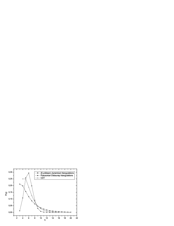
Figure 2: Comparing the probability distributions $P(q)$ of the vertex coordination numbers $q$ for three different types of random triangulations: Euclidean dynamical triangulations [30], Poissonian Delaunay triangulations [31] and causal dynamical triangulations [10].

The main idea is to use this distribution, together with some information about correlations between distributions at different vertices, to re-express the sum over triangulations in the high-temperature expansion of the partition function, (8), by an average over coordination numbers. In terms of geometric randomness, the pure CDT model lies in between the Voronoi-Delaunay triangulations based on Poissonian random distributions of vertices and the planar triangulations underlying the approach of Euclidean dynamical triangulations. A comparative plot of the probability distributions for the coordination numbers in the three different types of geometry is shown in Fig. 2.

Let us point out a further subtlety which arises from the fact that the underlying lattices are not fixed, but fluctuating, and therefore do not have a fixed “shape”. In this case it can happen that in the graph counting for the high-temperature expansion of some thermodynamic quantity topologically non-trivial graphs must be taken into account. By this we mean closed non-contractible graphs which wind around the spacetime. This does not invalidate the method in principle, but requires a more detailed knowledge of the global properties of the spacetime. In two-dimensional CDT, where the spacetime topology is usually chosen to be that of a cylinder (a spatial circle moving in time), this would be closed loop graphs which wind one or more times around the spatial $S^{1}$, and might be as short as a single link. Such pinching configurations certainly exist, but their contribution to the graph counting has been shown to be irrelevant in CDT, because it is subleading in $N$ in the thermodynamic limit [10].

4 Graph embeddings

4.1 Terminology of graph theory and embeddings

To prepare the ground for our counting prescription, we will first review some of the relevant terminology of graph theory and embeddings, along the lines of reference [32].

A linear graph is a collection of $v$ vertices and $l$ lines (or edges) connecting pairs of vertices. A simple graph is a graph in which two vertices are connected by at most one line and in which single lines are not allowed to form closed loops. A graph is said to be connected if there is at least one path of lines between any two vertices, and disconnected if for some vertex pair there is no such path.

The cyclomatic number $c$ of a connected graph $g$ is defined as

$$c(g)=l-v+1,$$ (11)

and represents the number of independent cycles in the graph.

The degree (or valence or coordination number) of a vertex is the number of edges incident on that vertex.

Two graphs are said to be isomorphic if they can be put into one-to-one correspondence in such a way that their vertices and edges correspond. They are called homeomorphic if they are isomorphic after insertion or suppression of any number of vertices of degree 2 (this operation being defined on an edge in a trivial way).

Homeomorphs are thus graphs with the same topology, in particular, with the same cyclomatic number. It is then possible to classify graphs in terms of irreducible graphs. An irreducible graph is one in which all vertices of degree 2 have been suppressed. (Note that in general it will no longer be a simple graph since it will contain single-line loops.) Typical irreducible graphs whose homeomorphs we will encounter are tadpoles, dumbbells, figure eights and $\theta$-graphs (Fig. 3).

Figure 3: Four kinds of homeomorphs: (a) tadpole, (b) dumbbell, (c) figure eight, and (d) $\theta$-graph.

In the high-temperature expansion of an Ising model it is useful to think of the lattice with its $v$ vertices and $l$ edges as a graph $G$. The graphs appearing in the expansion of the thermodynamic function of interest are then graphs embedded in $G$. A general definition of embeddings of graphs is the following. Let $G$ be a general graph. A graph $H$ is a subgraph of $G$ when all its vertices and edges are vertices and edges of $G$. An embedding of a graph $g$ in $G$ is a subgraph $G^{\prime}$ of $G$ which is isomorphic to $g$.

The lattice constant $(g;G)^{(N)}$ of a graph $g$ on $G$ is defined as the number of different embeddings of $g$ in $G$. In practice it is often useful to work with the lattice constant per site, defined as $(g;G)=\frac{2}{N}(g;G)^{(N)}$.

With these definitions in hand we can now rewrite the function $F^{(N)}(u,\tau)$ introduced in (7) as

$$F^{(N)}(u,\tau)\equiv 1+\sum_{s=0}^{\infty}\sum_{l>0}D_{l,2s}^{(N)}u^{l}\tau^{2s},$$ (12)

where $D_{l,2s}^{(N)}$ are the lattice constants of graphs of length $l$ and with $2s$ odd vertices, for which $F^{(N)}(u,\tau)$ serves as a generating function. It follows from the extensive nature of the free energy of the system that in the thermodynamic limit

$$F^{(N)}(u,\tau)\stackrel{{\scriptstyle N\rightarrow\infty}}{{\longrightarrow}}{\rm e}^{N\Theta(u,\tau)}=1+N\Theta(u,\tau)+O(N^{2}),$$ (13)

where the function $\Theta(u,\tau)$ does not depend on $N$. From the usual combinatorial theory of non-embedded graphs it is well known that the logarithm of the generating function is the generating function for connected graphs. Because of the embedded nature of the graphs in the case at hand, the disconnected graphs will still contribute to $\log F^{(N)}(u,\tau)$ with a “repulsion” term of sign $(-1)^{(\#connected\ components)-1}$.

In our analysis of the Ising model on CDT we will be looking at a quantum-gravitational average of the magnetic susceptibility at zero external field. For the usual Ising model the susceptibility $\chi$ per unit volume is given by

$$\chi(u)=\frac{1}{N}\frac{\partial^{2}\ln Z_{N}}{\partial H^{2}}_{\big{|}H=0}=\frac{1}{2}+\frac{2}{N}\frac{\sum_{l}D_{l,2}^{(N)}u^{l}}{1+\sum_{l}D_{l,0}^{(N)}u^{l}},$$ (14)

where in the second step we have substituted in the high-temperature expansion of the partition function. By virtue of (13) it is clear that the susceptibility is independent of $N$ in the infinite-volume limit (thus justifying our notation $\chi(u)$), and that moreover the denominator in the last term in (14) does not contribute at lowest order in $N$, which is the one relevant to the computation. To calculate the susceptibility, it is therefore sufficient to compute the term of order $N$ in $\sum_{l}D_{l,2}^{(N)}u^{l}$, as is well known.

The computation in the gravity-coupled case proceeds completely analogously. Performing the sum over all triangulations at fixed $N$, as in eq. (8), and then letting $N\rightarrow\infty$, one obtains

$$\chi_{\rm CDT}(u)\approx\frac{2}{N}\,\frac{\sum_{l}\left(\sum_{T_{N}}D_{l,2}^{(N)}(T_{N})\right)u^{l}}{\sum_{T_{N}}1+\sum_{l}\left(\sum_{T_{N}}D_{l,0}^{(N)}(T_{N})\right)u^{l}}=\frac{2}{N}\,\frac{\sum_{l}\langle D_{l,2}^{(N)}\rangle u^{l}}{1+\sum_{l}\langle D_{l,0}^{(N)}\rangle u^{l}}$$ (15)

for the susceptibility in presence of the gravitational CDT ensemble, where we have dropped the irrelevant constant term and introduced an obvious notation for the ensemble average in the second step. Whereas it was fairly straightforward to verify the cancellations of terms of higher order in $N$ between numerator and denominator in the pure Ising case in eq. (14) by an explicit calculation, the analogous computation does not seem feasible in the gravity-coupled case, although we know from the same general arguments that it must be realized here too. Again the terms in the denominator of the expressions on the right-hand side of (15) do not contribute at lowest order, which – at least for this particular observable – implies that its annealed and quenched gravitational averages coincide.

4.2 Useful results on lattice constants

We now want to identify which graph topologies appear in the high-temperature expansion of the magnetic susceptibility. For convenience we can divide our set of graphs into two subsets, graphs with zero cyclomatic number (also called Cayley trees), and graphs with $c>0$. Since the graphs we encounter in the susceptibility series must have two and only two odd vertices, it follows that the first subset will only contain connected non-selfintersecting open chains (in other words, self-avoiding walks), while the second will contain everything else. The connected graphs in the second subset are graphs with loops and one or no open ends, while the disconnected ones take the form of a union of one of the previous two kinds with any number of even graphs (graphs in which every vertex has even degree).

The problem we meet in the high-temperature expansion is the evaluation of the lattice constants of such graphs. It turns out that there are two kinds of theorems which can be applied profitably in the context of our random triangulated lattices. The first is very general and reduces the calculation of the lattice constants for disconnected graphs into that for connected graphs. This makes it possible to compute the lattice constants for the second subset ($c>0$) in a unified way. The second theorem is less general but powerful, since it gives us a recurrence relation for the expansion coefficients of the susceptibility.

The reduction theorem for disconnected graphs states that if $g_{i}$ and $g_{j}$ are two graphs $g_{i}\neq g_{j}$ and $G$ is any graph, then

$$(g_{i}\cup g_{j};G)=(g_{i};G)(g_{j};G)-\sum_{k}\{g_{i}+g_{j}=g_{k}\}(g_{k};G),$$ (16)

where $g_{i}\cup g_{j}$ stands for the disjoint union of the two graphs, $\{g_{i}+g_{j}=g_{k}\}$ is the number of possible choices of embeddings of $g_{i}$ and $g_{j}$ in $g_{k}$ having $g_{k}$ as their sum graph, and the summation is over all graphs $g_{k}$ obtainable in this way. If $g_{i}=g_{j}$ we can compute the right-hand side of (16) as if the two graphs had different colours and thus obtain $2(g_{i}\cup g_{i};G)$. If $g_{i}$ or $g_{j}$ are themselves non-connected graphs we can iterate the theorem. In this way the lattice constant of the disconnected union of $n$ connected graphs can be expressed as a polynomial of order $n$ in the lattice constants of connected graphs (see Fig. 4 for some simple examples).

Figure 4: Two examples of the reduction theorem. The graph $G$ has been dropped in the notation.

The counting theorem for the susceptibility series was first given by Sykes [33] in 1961, but only later proved by Nagle and Temperley [34] as a special case of a more general theorem of graph combinatorics. Closer examination reveals that the proof makes no reference to the structure of the lattice, but only to its coordination number $q$, which will turn out to be useful when considering the lattice dual to the triangulation. The theorem states that the high-temperature series for the susceptibility can be written as

$$\chi(u)=1+(1-\sigma u)^{-2}\left[qu(1-\sigma u)-2(1-u^{2})S_{1}+8(1+u)^{2}(S_{2}+S_{3})\right],$$ (17)

where $q=\sigma+1$ is the coordination number, and the functions $S_{i}$ are defined as

$$\begin{split}S_{1}&=\sum_{l>0}ld_{l}u^{l},\\ S_{2}&=\sum_{l>0}\left[\sum_{w>0}wd_{l}(w)\right]u^{l},\\ S_{3}&=\sum_{l>0}\left[\sum_{r\leq r^{\prime}}rr^{\prime}m_{l}(r,r^{\prime})\right]u^{l}.\end{split}$$ (18)

The coefficient $d_{l}$ is the sum of lattice constants of even graphs with $l$ lines, while $d_{l}(v)$ is restricted to even graphs with $l$ lines and vertices of degree $2q_{1},2q_{2},...$, characterized by the weight $w=\sum_{i}q_{i}(q_{i}-1)/2$. The function $m_{l}(r,r^{\prime})$ is the sum of lattice constants of graphs with exactly two odd vertices of degrees $2r+1$ and $2r^{\prime}+1$. Substituting the left-hand side of formula (17) by the expansion $\chi(u)=1+\sum_{n>0}a_{n}u^{n}$, one finds a recursive relation for the coefficients $a_{n}$, namely,

$$\begin{split}a_{l}-2\sigma a_{l-1}&+\sigma^{2}a_{l-2}=2(l-2)d_{l-2}-2ld_{l}+\\ &+8\left[\sum_{w>0}wd_{l}(w)+2\sum_{w>0}wd_{l-1}(w)+\sum_{w>0}wd_{l-2}(w)\right]+\\ &+8\left[\sum_{r\leq r^{\prime}}rr^{\prime}m_{l}(r,r^{\prime})+2\sum_{r\leq r^{\prime}}rr^{\prime}m_{l-1}(r,r^{\prime})+\sum_{r\leq r^{\prime}}rr^{\prime}m_{l-2}(r,r^{\prime})\right].\end{split}$$ (19)

As a result, at every new order $l$ in our calculation the only new lattice constants we have to evaluate are those for graphs with no vertex of degree 1, reducing the computational effort considerably.

This formula can in principle be applied to any non-regular lattice whose vertices are all of the same degree. For a fixed non-regular lattice this observation would usually not be of much help, because one would still need to compute at each order the new lattice constants depending on the complete, detailed information of the lattice geometry. In our case this difficulty is not present, since we are summing over triangulations and can simply substitute in (19) the lattice constants averaged over the triangulations, without the need of keeping track of the lattice geometry for individual lattices.

4.3 Counting graphs on the CDT triangular lattice

Next, we will analyze the evaluation procedure for lattice constants in the quantum-gravitational CDT model. Computations here are made difficult by the randomness of the coordination number. At the outset it is not even obvious that any of the known recurrence relations can be used. Our task is to list all possible diagrams, and for each count the number of ways it can be embedded in the lattice. On a regular lattice such an operation is tedious but straightforward: starting from a fixed vertex, we trace out all possible sequences of links of a given length, say, which do not self-intersect. The discrete symmetries of the regular lattice simplify this task greatly. In the simplest case, the counting has to be done only for a single initial vertex, with all other graphs obtained subsequently by translational symmetry. The analogous counting on the dynamical CDT lattices is complicated by the fact that the lattice neighbourhoods of different vertices will in general look different. We will deal with this difficulty by setting up an algorithm to count the embedding of a given diagram on the ensemble of CDT lattices, making use of the known probability distribution of the vertex coordination numbers.

Before presenting this algorithm we need some more notation. CDT lattices have two kinds of links, time-like and space-like. In keeping with the usual representation of two-dimensional CDT lattices (c.f. Fig. 1, left-hand side), we will draw time- and space-like links in embeddings of graphs as (diagonally) upward-pointing and horizontal lines, respectively (see Fig. 5). Furthermore we need to keep track of the relative up-down or right-left orientation of consecutive links, to distinguish between graphs like (c) and (d) in Fig. 5 (which give different contributions to the lattice constant). In addition, the counting for a graph like (b) will be identical to that for its mirror images under left-right and up-down reflections. These mirrored graphs will be counted by multiplying the embedding constant of the graph by an appropriate symmetry factor.

Figure 5: The possible typologies of embedding, up to reflection symmetry, of a length-2 open chain. The angle which the time-like links form with the vertical has no relevance for the graph counting.

A symmetry factor 1 is assigned to graphs symmetric under both up-down and left-right reflections (for example, graphs $(a)$ and $(d)$), a factor 2 to graphs with only one of the two symmetries (like graph $(c)$) or symmetric with respect to a composition of the two (like graph $(c)$ of Fig. 6), and a factor 4 to graphs without reflection symmetry (like graph $(b)$ of Fig. 5 or $(a)$ and $(b)$ of Fig. 6).

Figure 6: Three of the different typologies of possible embeddings of a length-3 open chain.

The lattice constant $(g;T)$ of a graph $g$ embedded in a graph corresponding to a triangulation $T$ is computed as

$$(g;T)=\sum_{i}s_{i}(g;T)_{i},$$ (20)

where $(g;T)_{i}$ is the number of ways a particular typology of embedding $(g)_{i}$ can be realized on $T$, $s_{i}$ is the relevant symmetry factor, and the sum extends over all possible typologies of embeddings of the graph $g$. In the context of quantum gravity, we are interested in the average of (20) over all triangulations, that is,

$$\langle g\rangle=\frac{\sum_{T}(g;T)}{\sum_{T}1},$$ (21)

which will take into account the probability distribution of the vertex coordination.

As mentioned earlier, all calculations will be performed in the thermodynamic limit where the cosmological constant is tuned to its critical value $\lambda_{c}=\ln 2$. In this limit, the probability of having $k$ incoming time-like links at a particular lattice vertex is given by

$$p(k)=\frac{1}{2^{k}},$$ (22)

with an identical probability for having $k$ outgoing time-like links at a vertex. Moreover, at one and the same vertex the two probabilities are independent of each other. In fact, not just for a single vertex are these two probabilities independent, but the same is true for all vertices lying in the same space-like, horizontal slice. By contrast, the outgoing probability at a vertex will in general condition the incoming probability at another vertex on the subsequent horizontal slice. By construction, the probability of having a space-like link to the left and to the right of an given vertex is equal to 1.

Armed with this information we are now ready to compute any of the $(g;G)_{i}$ in (20). We do not have a general counting formula in closed form, but will formulate a number of rules and tools which will enable us to do the counting recursively. We will start with some illustrative examples. Examples 3 and 4 will serve as our elementary building blocks in more complicated constructions.

Example 1. The simplest example is that of a length-1 graph $c_{1}$, consisting of a single horizontal or vertical link. The number of horizontal embeddings is the number of horizontal links on a CDT lattice, which by virtue of the Euler relation is given by half the number of triangles, i.e. $N/2$. If we give the lattice constant per vertex, as is customary in the literature, it is therefore $\langle c_{1}\rangle_{h}=1$. By a similar topological argument we can immediately deduce the number 2 for the lattice constant of vertical embeddings, but it is instructive to compute it from the probability distribution (22) instead. If at a vertex we have $k$ outgoing vertical links, there are precisely $k$ ways to embed the one-link graph such that it emanates in upward direction from this vertex. Since every vertical embedding is accounted for in this way, by assigning the relevant probability and summing over $k$ we obtain

$$\langle c_{1}\rangle_{v}=\sum_{k=1}^{\infty}\frac{k}{2^{k}}=2,$$ (23)

in agreement with the earlier argument. The total contribution to the lattice constant at order 1 is therefore $\langle c_{1}\rangle_{h}+\langle c_{1}\rangle_{v}=3$.

Example 2. Next, let $c_{2}$ be a length-2 open chain, and consider the embedding typology $c_{2,b}$ shown in Fig. 5$(b)$. The result follows straightforwardly from example 1: there is one horizontal link per vertex, and there are in the ensemble on average two ways of attaching an outgoing vertical line to its right vertex, yielding $\langle c_{2}\rangle_{b}=2$. For the embedding of Fig. 5$(a)$ there is nothing to compute; we have $\langle c_{2}\rangle_{a}=1$. The embedding of Fig. 5$(d)$ is the first configuration we encounter which extends over two triangulated strips. Because of the independence of the probabilities (22) in successive strips we obtain

$$\langle c_{2}\rangle_{d}=(\sum_{k=1}^{\infty}\frac{k}{2^{k}})^{2}=4.$$ (24)

Example 3. Now consider the embedding $c_{2,c}$ depicted in Fig. 5$(c)$. If the vertex on top has $k$ incoming links, there are exactly $k(k-1)/2$ ways to realize the embedding, leading to

$$\langle c_{2}\rangle_{c}=\sum_{k=1}^{\infty}\frac{k(k-1)}{2^{k+1}}=2.$$ (25)

Note that the same “inverted-V” embedding on a flat triangular lattice $T_{\rm reg}$ would give $(c_{2};T_{\rm reg})_{c}=1$ instead. Putting everything together and multiplying by the appropriate symmetry factors we get $\langle c_{2}\rangle_{a}+4\langle c_{2}\rangle_{b}+2\langle c_{2}\rangle_{c}+\langle c_{2}\rangle_{d}=17$ as a total contribution at order 2.

In view of more complicated graphs, an alternative and more convenient way of doing the calculation in example 3 is by focussing on the probability distributions of the vertices lying on the lower space-like slice of the triangulated strip (see also Fig. 7$(a)$). The probability of having $n$ space-like links in between the two vertices at the ends of the inverted V is given by the probability that there are $n-1$ vertices in between with precisely one outgoing link each, which is $1/2^{n-1}$. Thus we obtain again

$$(c_{2};G)_{c}=2\sum_{n=1}^{\infty}\frac{1}{2^{n-1}}=4.$$ (26)

Figure 7: Two configurations contributing to the calculations of examples 3 and 4. The labels m and n count the numbers of space-like links as indicated.

Example 4. Consider an open chain of length greater than 2 embedded in such a way that only the first and last edges lie along time-like links, with a horizontal chain of $m$ space-like links in between. Both time-like links are supposed to lie in the same strip of the triangulation, as illustrated in Fig. 7$(b)$. We are going to prove that the lattice constant of such a configuration is given by

$$\langle c_{m+2}\rangle_{b}=\sum_{n=1}^{\infty}\frac{1}{2^{m+n-1}}\begin{pmatrix}m+n\\ m\end{pmatrix}=4-2^{1-m}.$$ (27)

The result $4-2^{1-m}$ could be obtained easily by (i) considering the number of ways in which each of the two vertices at the top left and right can have an incoming link (giving a total of $2\times 2=4$ possibilities) and (ii) subtracting from that the probability for the two time-like links touching each other in their lower vertex, which is $2^{1-m}$ (the probability that the $m-1$ intervening vertices have only one incoming link each). However, we rather want to do the counting in a way that keeps track of the number of links separating the two vertices at the bottom, for reasons that will become clear soon. In other words, we want to determine the lattice constant for a closed polygon consisting of two vertical edges, $m$ edges along the top and $n$ along the bottom. From a combinatorial point of view this can be rephrased as the problem of counting the number of different ways in which $n$ triangles and $m$ upside-down triangles can be arranged to form a strip, with the well-known binomial result $\big{(}{m+n\atop m}\big{)}$. To get the lattice constant for our random lattice we still have to include a probabilistic factor $\frac{1}{2}$ for each vertical link in the polygon interior, leading to the factors $2^{1-m-n}$ in formula (27).

The strips decomposition. The embedding typology $(g)_{i}$ of any connected graph $g$ extends over a well-defined number of strips in the CDT triangulation, and each part of $(g)_{i}$ belongs to a definite strip or horizontal slice. Our first step in the counting procedure is to decompose the embedded graphs into strip contributions, thus breaking the graph into pieces. The example of Fig. 8 will help us explain the procedure. It shows a particular embedding of $c_{4}$, how it is decomposed into two pieces, and how its lattice constant can be computed accordingly. All we have to do is multiply the probability of $c_{2,c}$ (example 2) with $m$ links at the bottom with the probability of $c_{m+2,b}$ (example 3), and then sum over $m$, resulting in

$$\langle c_{4}\rangle_{x}=\sum_{m=1}^{\infty}\frac{1}{2^{m-1}}(4-2^{1-m})=\frac{20}{3}.$$ (28)

Figure 8: Example of a strip decomposition. The embedding on the left is split into two strips, after which the strip contributions for given $m$ are multiplied pairwise and summed over.

We can think of this operation as a product of an (infinite-dimensional) vector and matrix,

$$\begin{split}K_{1}(m)&=\frac{1}{2^{m-1}},\\ K_{2}(m,n)&=\frac{1}{2^{m+n-1}}\begin{pmatrix}m+n\\ m\end{pmatrix},\end{split}$$ (29)

followed by taking the trace in order to impose the open boundary condition, that is,

$$\langle c_{4}\rangle_{x}={\rm Tr}(K_{1}\cdot K_{2}).$$ (30)

Fig. 8 is a simple case with only two vertical lines in each strip. In general there will be more lines, like in Fig. 9. However, there are only two possibilities for pairs of neighbouring vertical links: they can be either disjoint or have exactly one vertex in common, so that the probability associated with them in a particular embedding in a particular triangulation will be given by either $K_{2}(m,n)$ or $K_{1}(n)$. We can then associate a probability to a given pattern of vertical lines in a strip with fixed distance between them (in terms of the horizontal links in the in- and out-slice), which is the product of the corresponding $K_{1}$- or $K_{2}$-probabilities, times a factor $\frac{1}{2}$ for each shared vertical line between two neighbouring $K_{i}$-patterns in the same strip (see Fig. 9). In the end we have to glue the strips back together again, with conditions such as to get the desired graph, and sum over the allowed values of horizontal lengths. As an illustrative example, we obtain for Fig. 9 the multiple sum

$$\sum_{j_{1}=1}^{\infty}\sum_{m_{1}=1}^{\infty}\sum_{m_{2}=2}^{\infty}\sum_{j_{2}=1}^{m_{2}-1}\sum_{n=1}^{\infty}[K_{2}(l_{1}+j_{1},m_{1})\frac{1}{2}K_{2}(l_{2},m_{2})][K_{1}(m_{1})\frac{1}{2}K_{2}(m_{2}-j_{2},n)\frac{1}{2}K_{1}(j_{2})],$$ (31)

where we have grouped the factors corresponding to the same strip in square brackets. As should be clear from this example, the gluing and the range of the summations for the various graph embeddings will have to be taken care of on a case-by-case basis.

Figure 9: Example of a more complicated strip decomposition where each strip consists of a sequence of elements of the kind illustrated in Fig. 7. The sum refers to the total sum in the expression (31) which has to be performed after the proper weights have been assigned to each element of the graph.

Using these techniques we have repeated and independently confirmed the calculation of the first five orders given in [10] and then extended it to order 6. Table 1 gives the lattice constants (times 2) per number of vertices (which we will call the susceptibility coefficients) of the open chains, the other graphs, and of their grand total. The effort involved in this extension is by no means minor. There are 387 order-6 open chains that have to be counted individually, with the identifications introduced in this section, and for many of them the computation requires a careful use of the strip decomposition and a subsequent evaluation of the sums involved.

$n$	open	closed + disconnected	total ($a_{n}$)
1	6	0	6
2	34	0	34
3	174	0	174
4	$859\frac{1}{3}$	$-12$	$847\frac{1}{3}$
5	$4152\frac{2}{3}$	$-162\frac{2}{3}$	3990
6	$19800\frac{19}{27}$	$-1416\frac{1}{9}$	$18384\frac{16}{27}$

Table 1: Susceptibility coefficients for the CDT lattice up to order 6. The terminology ‘open’, ‘closed’ and ‘disconnected’ refers to the topology of the graphs.

4.4 Counting graphs on the dual CDT lattice

On the dual lattice (an example of which is depicted in Fig. 1, right-hand side) we can apply formula (19), which for $q=3$ reduces to

$$\begin{split}a_{l}-4\sigma a_{l-1}+4a_{l-2}&=2(l-2)d_{l-2}-2ld_{l}+\\ &+8\left[m_{l}(1,1)+2m_{l-1}(1,1)+m_{l-2}(1,1)\right].\end{split}$$ (32)

Because of the low coordination number the only even graphs that can appear are connected or disconnected polygons, and the only contributions to $m_{l}$ are from $\theta$-graphs and dumbbells with or without disconnected polygonal components. For the disconnected graphs we can use the reduction theorem. It should be noted that in the overlap decomposition new topologies of graphs appear, for example, graphs with more than two odd vertices, still rendering the higher-order computations non-trivial.

It is not difficult to derive the probability distribution relevant for the dual lattice from the one of the original lattice. The probability of having two horizontal links at a vertex, one to the right and one to the left, is again 1. The probability for an incoming or outgoing vertical link at a vertex of a given chain of horizontal links is given by the probability of having a triangle or an upside-down triangle in the corresponding strip of the original triangulation. Since the two cases are mutually exclusive, the in- and out-probabilities are not independent and each takes the value $1/2$, which may also be thought of as the weight associated with a triangle in the original lattice. With these rules the lattice constant of an open chain of length 1 is $3/2$: 1 for the horizontal link (associated to its left vertex, say, in order to avoid overcounting), plus $1/2$ for the vertical link. Alternatively, this easy example can be computed by use of the Euler relation. For higher-order graphs it is often convenient to go back to the original lattice and count – with the appropriate weights – the configurations which can be associated to the dual graph under consideration.

Example 1. Let us consider again a closed polygon with only two vertical links, with $m$ links on the top and $n$ on the bottom, but this time on the dual CDT lattice (see Fig. 10). A careful evaluation of the probabilities involved yields

$$\langle c_{m,n}\rangle^{*}=\frac{1}{2^{m+n+1}}\sum_{k=0}^{min(m,n)-1}\begin{pmatrix}m-1\\ k\end{pmatrix}\begin{pmatrix}n-1\\ k\end{pmatrix}$$ (33)

for its lattice constant, where $k$ is the number of vertical links of the lattice which lie inside the polygon, and $\langle\cdot\rangle^{*}$ denotes the average lattice constant per vertex of the dual graph. The binomials in (33) count the number of possible ways to arrange the $k$ internal links, and the remaining probability – expressed as a power of $1/2$ – turns out not to depend on $k$.

Figure 10: An embedding of the polygon considered in example 1.

As already mentioned, the in-and out-probabilities at a vertex of the dual lattice are not independent, which means that we cannot apply the strip decomposition of the original lattice directly, but instead have to proceed more carefully.

Example 2. As an example of this, consider a polygon embedding that extends over two strips (Fig. 11), a type of configuration that appears from order 8 onward. Its lattice constant is given by

$$\begin{split}\langle c_{m_{1},m_{2},n_{1},n_{2}}\rangle^{*}&=\sum_{k_{1}=0}^{m_{1}-1}\begin{pmatrix}m_{1}-1\\ k_{1}\end{pmatrix}\sum_{k_{2}=0}^{m_{2}-1}\begin{pmatrix}m_{2}-1\\ k_{2}\end{pmatrix}\times\\ &\times\sum_{i=0}^{min(k_{1},n_{1}+n_{2}-4)}\begin{pmatrix}k_{1}-i+k_{2}\\ k\end{pmatrix}\begin{pmatrix}n_{1}+n_{2}-2\\ i\end{pmatrix}\frac{1}{2^{m_{1}+m_{2}+n_{1}+n_{2}+k_{1}-i+k_{2}+2}}.\end{split}$$ (34)

In eq. (34), $m_{1}$ and $m_{2}$ count the links on the top and bottom horizontal lines, and $n_{1}$ and $n_{2}$ count the two sets of contiguous links on the central horizontal line. The numbers of internal vertical links in the upper and lower strip are denoted by $k_{1}$ and $k_{2}$, while $i$ counts how many links out of the $k_{1}$ end on one of the two intermediate horizontal lines. The logic behind the various counting factors appearing under the sums is very similar to that of the previous example.

Figure 11: An embedding of the polygon considered in example 2.

We have found the method illustrated by examples 1 and 2 the most compact one to deal with the counting of graph embeddings on the dual CDT lattice. It has enabled us to push our “counting by hand” to order 12, the results of which are given in Table 2. Because of the fixed, low coordination number of the dual vertices, there are far fewer graphs at a given order than there are on the original CDT lattice.

$n$	1	2	3	4	5	6	7	8	9	10	11	12
$a_{n}$	3	6	12	23	42+$\frac{3}{4}$	78+$\frac{1}{2}$	142+$\frac{3}{4}$	258	461+$\frac{13}{16}$	820+$\frac{1}{8}$	1446+$\frac{13}{32}$	2532+$\frac{11}{16}$

Table 2: Susceptibility coefficients for the dual CDT lattice up to order 12.

5 Series analysis

5.1 Review of different methods

Having computed the two high-temperature series to some order, we will now turn to analyzing them, and try to extract information on the critical properties of the underlying gravity-matter systems. The standard analytic methods are well-known from the case of regular lattices and reviewed in [35]. We will recall them briefly here in order to be self-contained.

The first and most straightforward tool is that of the ratio method, which works as follows. Assuming a simple behaviour of the susceptibility of the form

$$\chi(u)\sim A(u)\Bigl{(}1-\frac{u}{u_{c}}\Bigr{)}^{-\gamma}+B(u)$$ (35)

near the critical point $u_{c}$, with analytic functions $A$ and $B$, its series expansion $\chi(u)=1+\sum_{n>0}a_{n}u^{n}$ should yield (to first order in $1/n$)

$$r_{n}\equiv\frac{a_{n}}{a_{n-1}}=\frac{1}{u_{c}}\Bigl{(}1+\frac{\gamma-1}{n}\Bigr{)}.$$ (36)

One can then generate sequences of estimates of the critical parameters from sequences of point pairs $\{r_{n},r_{n-1}\}$ [35], namely,

$$\gamma_{n}=\frac{n(2-n)r_{n}+(n-1)^{2}r_{n-1}}{nr_{n}-(n-1)r_{n-1}},$$ (37)

$$u_{c,n}=\frac{1}{nr_{n}-(n-1)r_{n-1}}.$$ (38)

In general, these will converge very slowly. In addition, if the series has an oscillatory behaviour the method can yield alternating over- and underestimates. In this case a fit of a whole sequence $\{r_{min},...,r_{max}\}$, computed with the help of (36), may be better suited than the sequence of estimates to find the straight line masked by the oscillations ($r_{min}$ is chosen properly to exclude large deviations from (36) at small $n$, and $r_{max}$ is the ratio computed for $n=n_{max}$).

Oscillations and other irregularities in the expansion are caused by a more complicated behaviour of the thermodynamic function, for example, the presence of other singularities in the complex plane close to the physical singularity, which in unfortunate cases may even lie closer to the origin than the singularity of interest. In case the behaviour near the physical singularity is like

$$\chi(u)\sim A(u)\Bigl{(}1-\frac{u}{u_{c}}\Bigr{)}^{-\gamma},$$ (39)

with $A(u)$ a meromorphic function with singularities close to $u_{c}$, a method that should give better results than the ratio method is that of the so-called Padé approximants. The method consists in the approximation of a function, known through its series expansion to order $\cal N$, by a ratio of two polynomials of order $\cal L$ and $\cal M$, subject to the condition $\cal L+M\leq N$,

$$\frac{P_{\cal L}(x)}{Q_{\cal M}(x)}\equiv\frac{\sum_{k=0}^{\cal L}p_{k}x^{k}}{1+\sum_{k=1}^{\cal M}q_{k}x^{k}}=F_{\cal N}(x)+O(x^{{\cal L+M}+1})$$ (40)

with $F_{\cal N}(x)=\sum_{k=0}^{\cal N}a_{k}x^{k}$. By common usage, the notation $\cal[L/M]$ indicates the order of the polynomials used.

In our specific case one takes as the function $F(x)$ to be approximated the derivative of the logarithm of $\chi(u)$, so that $u_{c}$ can be recognized as a pole and $\gamma$ as the associated residue in

$$\frac{d}{du}\log\chi(u)=\frac{\gamma}{u_{c}-u}\left(1+O(u_{c}-u)\right).$$ (41)

This is also referred to as the Dlog Padé method. Usually one only looks at the tridiagonal band $[({\cal N}-1)/{\cal N}]$, $\cal[N/N]$ and $[({\cal N}+1)/{\cal N}]$ because of the invariance of the diagonal Padé approximants under Euler transformations.

The Padé approximants work well only when there is no additive term $B(u)$. In presence of such a term there is a generalization – known as differential approximants – to account for functional behaviours of the form

$$\chi(u)\sim\prod_{i=1}^{n}A_{i}\Bigl{(}1-\frac{u}{u_{i}}\Bigr{)}^{-\gamma_{i}}+B(u),$$ (42)

with $B(u)$ and $A_{1},...,A_{n}$ analytical functions and $u_{1},...,u_{n}$ a set of singular points. If we are considering the logarithmic derivative of a function $f(x)$ we can rewrite (40) as

$$P_{\cal L}(x)f(x)-Q_{\cal M}(x)f^{\prime}(x)=O(x^{{\cal L+M}+1}).$$ (43)

The idea of the differential approximants method is to generalize this equation according to

$$R_{{\cal M}_{2}}(x)F^{\prime\prime}_{\cal N}(x)+Q_{{\cal M}_{1}}(x)F^{\prime}_{\cal N}(x)-P_{\cal L}(x)F_{\cal N}(x)=S_{\cal K}(x)+O(x^{{\cal K+L}+{\cal M}_{1}+{\cal M}_{2}+1}),$$ (44)

where $R_{\mathcal{M}_{2}}(x)$ and $S_{\mathcal{K}}(x)$ are two other polynomials of order $\mathcal{M}_{2}$ and $\mathcal{K}$, and where one can substitute the differential operator by $D=x\frac{d}{dx}$, forcing the point at the origin to be a regular singular point. In the following we will only consider the special case $R_{\mathcal{M}_{2}}\equiv 0$, giving rise to the so-called inhomogeneous 1st-order differential approximant, denoted by $[\mathcal{K}/\mathcal{L};\mathcal{M}_{1}]$. With this method, the exponent $\gamma$ can be evaluated as

$$\gamma=\frac{P_{\mathcal{L}}(x_{c})}{x_{c}Q^{\prime}_{\mathcal{M}_{1}}(x_{c})},$$ (45)

where $x_{c}$ is a simple root of $Q_{\mathcal{M}_{1}}(x)$, which gives an estimate of the critical point.

5.2 The CDT lattice series

The high-temperature series expansion for the Ising susceptibility on the CDT model is given by

$$\chi_{\rm CDT}(u)=1+6u+34u^{2}+174u^{3}+(847+\frac{1}{3})u^{4}+3990u^{5}+(18384+\frac{16}{27})u^{6}+O(u^{7}).$$ (46)

Applying formulas (37) and (38) we get the sequence of estimates for $\gamma$ and $u_{c}$ reported in Table 3.

$n$	$u_{c}\hskip 28.45274pt$	$\gamma$
3	0.2489	1.819
4	0.2424	1.721
5	0.2459	1.791
6	0.2438	1.740

Table 3: Two-point linear extrapolations of the critical point and the critical exponent of the series (46) obtained using (37) and (38).

The results of linearly fitting the whole sequence of ratios $\{r_{2},...,r_{max}\}$ instead are listed in Table 4, and a plot of the ratios $\{r_{2},...,r_{6}\}$ versus $1/n$ together with their fit is shown in Fig. 12. Despite the shortness of the sequence, the linear fit is of very good quality.

$n_{\rm max}$	$u_{c}$	$\gamma$
3	0.2488	1.820
4	0.2462	1.789
5	0.2458	1.783
6	0.2454	1.779

Table 4: Linear fits of the sequences $\{r_{2},...,r_{max}\}$ for the series (46) with assumed functional form (36).

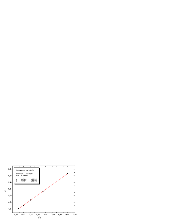
Figure 12: Plot of the ratios (36) for the case of the CDT lattice (data from Table 4).

It is worth noting that if we remove the point $r_{2}$, which of course is subject to the largest deviations from a pure $1/n$-behaviour due to higher-order terms, and fit the truncated sequence $\{r_{3},...,r_{6}\}$, we obtain $\gamma=1.749$ and $u_{c}=0.2441$ (see Table 5).

$n_{\rm max}$	$u_{c}$	$\gamma$
4	0.2424	1.721
5	0.2439	1.745
6	0.2441	1.749

Table 5: Linear fits of the sequences $\{r_{3},...,r_{max}\}$ for the series (46) with assumed functional form (36).

It is surprising how fast the ratio sequence seems to converge to the result $\gamma=1.75$ of the exact solution for the flat regular case, as compared to the analogous one obtained from the series expansion on the plane triangular lattice (see [36] for the expansion coefficients to order $u^{16}$), even though we cannot claim the result to be conclusive because of the limited number of terms at our disposal (see Fig. 13).

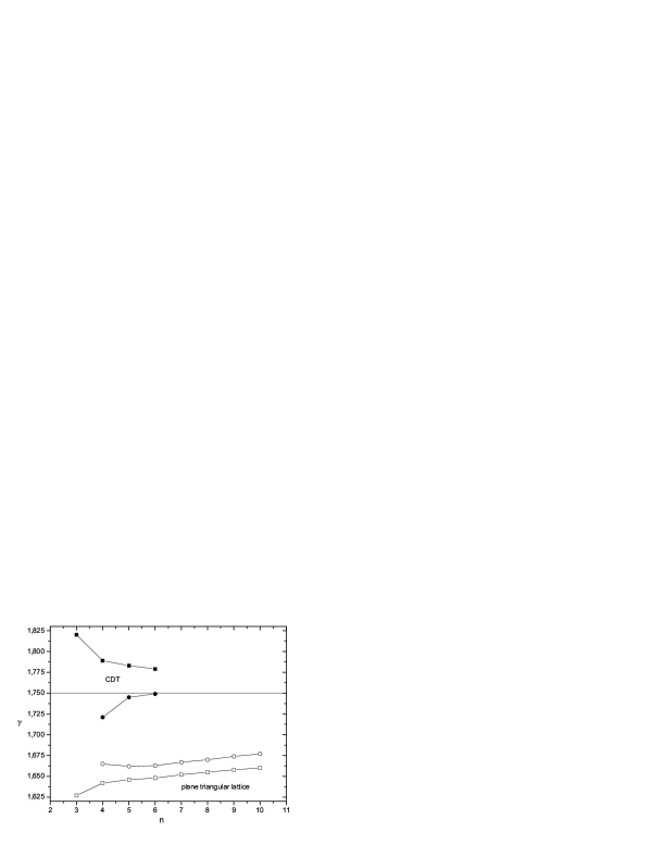
Figure 13: A comparative plot of estimates of the critical exponent $\gamma$ for the Ising model on the CDT versus that on a plane triangular lattice (data taken from [36]), obtained via the ratio method. The filled shapes refer to the CDT model and the open ones to the plane triangular lattice. The squares indicate fits of $\{r_{n_{min}},...,r_{n}\}$ sequences, and the circles those of sequences $\{r_{n_{min}+1},...,r_{n}\}$ with the first ratio eliminated.

What is the picture when we use one of the alternative methods to evaluate the series expansions? Results from the Dlog Padé and differential approximants methods are somewhat inconclusive, most likely because of the small number of estimates we can perform with our 6th-order series (see Table 6). To get a feel for what may be expected at this order, we report in Table 7 the corresponding Dlog Padé approximants $[({\cal N}+j)/\cal N]$ to the series for the plane triangular lattice (see again [36]). The estimates for the critical exponent $\gamma$ in the latter case are clearly closer to the known exact value, whereas for the CDT model, with only two values for the diagonal $\cal[N/N]$, it is quite impossible to extrapolate the behaviour of $\gamma$. (Note that we are reporting the estimates for the critical point $u_{c}$ only for completeness; they are or course not expected to coincide for the two models.) We have also computed the inhomogeneous first-order differential approximants $[{\cal L}/({\cal N}+j);\cal N]$ for the CDT series, which was defined just before formula (45). Values for the critical exponents are not completely off, but there are simply too few of them to make any statement about their convergence behaviour (see Table 8).

	$[({\cal N}-1)/{\cal N}]$		$[{\cal N}/{\cal N}]$		$[({\cal N}+1)/{\cal N}]$
${\cal N}$	$u_{c}$	$\gamma$	$u_{c}$	$\gamma$	$u_{c}$	$\gamma$
1	0.1875	1.125	0.2540	2.064	0.2513	2.000
2	0.2514	2.003	0.2483	1.8810	0.2517	2.008
3	0.2519	2.012	-	-	-	-

Table 6: Dlog Padé approximants method applied to the CDT series (46).

	$[({\cal N}-1)/{\cal N}]$		$[{\cal N}/{\cal N}]$		$[({\cal N}+1)/{\cal N}]$
${\cal N}$	$u_{c}$	$\gamma$	$u_{c}$	$\gamma$	$u_{c}$	$\gamma$
1	0.2500	1.500	0.2666	1.706	0.2678	1.730
2	0.2679	1.732	0.2670	1.712	0.2661	1.688
3	0.2662	1.692	0.2667	1.705	0.2672	1.722

Table 7: Dlog Padé approximants method applied to the plane triangular series in [36].

		${\cal N}=$
${\cal L}$	$j$	1	2
1	-1	$u_{c}=0.2143$	0.2454
		$\gamma=1.767$	1.815
	0	0.2373	0.2461
		1.568	1.832
	1	0.2496	-
		1.944	-
2	-1	0.2252	0.2463
		1.265	1.840
	0	0.2529	-
		2.087	-
	1	0.2431	-
		1.685	-
3	-1	0.2334	-
		1.361	-
	0	0.2402	-
		1.577	-
	1	-	-
		-	-
4	-1	0.2357	-
		1.396	-
	0	-	-
		-	-
	1	-	-
		-	-

Table 8: Inhomogeneous 1st-order differential approximants $[{\cal L}/({\cal N}+j);{\cal N}]$ method for the series (46).

5.3 The dual CDT lattice series

The high-temperature series expansion for the Ising susceptibility on the dual CDT model is given by

$$\begin{split}\chi_{\rm CDTd}(u)&=1+3u+6u^{2}+12u^{3}+23u^{4}+(42+\frac{3}{4})u^{5}+(78+\frac{1}{2})u^{6}+(142+\frac{3}{4})u^{7}\\ +&258u^{8}+(461+\frac{13}{16})u^{9}+(820+\frac{1}{8})u^{10}+(1446+\frac{13}{32})u^{11}+(2532+\frac{11}{16})u^{12}+O(u^{13})\end{split}$$ (47)

Using expressions (37) and (38) we get the sequence of ratio-method estimates for $\gamma$ and $u_{c}$ reported in Table 9.

$n_{\rm max}$	$u_{c}\hskip 28.45274pt$	$\gamma$
3	0.5	1.
4	0.6	1.6
5	0.6147	1.713
6	0.5800	1.390
7	0.5842	1.436
8	0.5782	1.360
9	0.6057	1.758
10	0.6064	1.769
11	0.6093	1.820
12	0.6202	2.033

Table 9: Two-point linear extrapolations of the critical point and the critical exponent of the dual series (47) obtained using (37) and (38).

The relative ratio plot is shown in Fig. 14, and shows gentle oscillations around the best linear fit of the sequence $\{r_{3},...,r_{12}\}$, leading to the estimates $\gamma=1.568$ and $u_{c}=0.5956$. However, these numbers do not tell it all. The strong qualitative differences with the planar honeycomb lattice, the appropriate non-random version of the dual CDT lattice, are illustrated in Fig. 15. It shows a comparative plot of the ratios extracted for the two models (the expansion coefficients for the honeycomb lattice, known to order $u^{32}$, can be found in [36]). Obviously, the influence of interfering unphysical singularities present on the regular honeycomb lattice is much reduced in the fluctuating dual CDT ensemble.

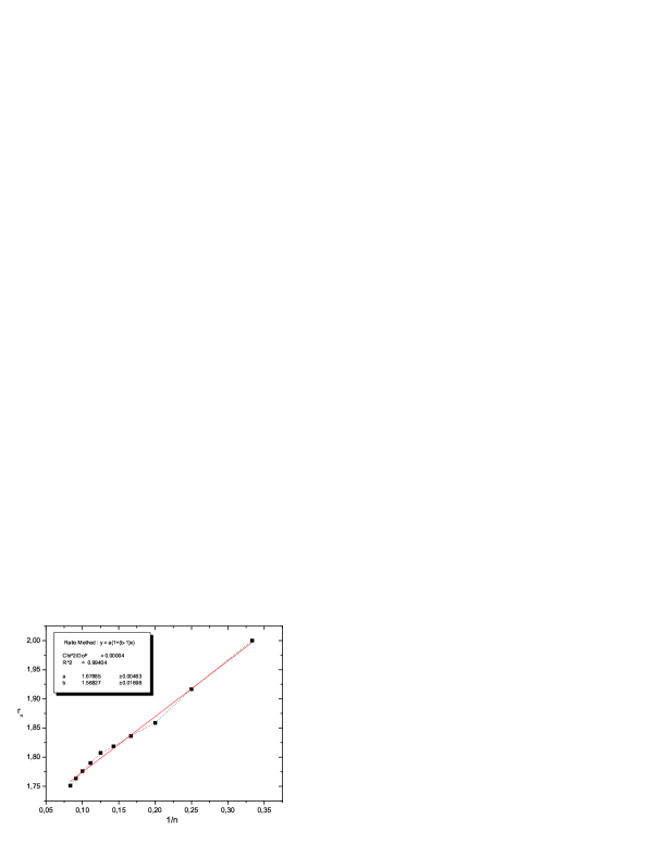
Figure 14: Plot of the ratios (36) for the case of the dual CDT lattice.

Figure 15: A comparative plot of the ratios of the regular honeycomb lattice (data taken from [36]) versus the dual CDT model.

On the basis of the rather well-behaved results for the Ising susceptibility on dynamically triangulated spacetimes we conjectured in [12] that “coupling to quantum gravity” may be an optimal method to learn about the critical behaviour of a matter or spin system, in the sense that the randomness of the underlying geometry eliminates spurious unphysical singularities (due to the presence of discrete symmetries in the case of regular lattices), but is not strong enough to change the universality class of the matter system. This is a dynamical version of similar conjectures made in the 1980s, which advocated the use of fixed random lattices to improve the convergence behaviour of lattice gauge theory, say (see, for example, [37]), but ultimately did not succeed.

If it is indeed the case that the singularity structure of the thermodynamic quantities in the complex plane is simplified, this could explain that the simple ratio method does indeed give the best result, at least at the relatively low orders we have been considering. In the case of the Ising model coupled to Euclidean dynamical triangulations, an analogous result has already been obtained with regard to the locus of the zeros of the partition function in the complex-temperature plane, where unphysical singularities of the flat regular lattices have been shown to be largely absent [38]. However, as already mentioned, the underlying geometries are too disordered to serve our present purpose, because their critical matter behaviour is changed compared to the flat case.

	$[({\cal N}-1)/{\cal N}]$		$[{\cal N}/{\cal N}]$		$[({\cal N}+1)/{\cal N}]$
${\cal N}$	$u_{c}$	$\gamma$	$u_{c}$	$\gamma$	$u_{c}$	$\gamma$
3	0.5952	1.554	0.5574	0.9738	0.5686	1.170
4	0.5691	1.180	0.5564	0.9567	0.5861	1.446
5	0.5890	1.492	0.5935	1.560	0.6359	2.996
6	0.5761	1.402	-	-	-	-

Table 10: Dlog Padé approximants method for the dual CDT series (47).

	$[({\cal N}-1)/{\cal N}]$		$[{\cal N}/{\cal N}]$		$[({\cal N}+1)/{\cal N}]$
${\cal N}$	$u_{c}$	$\gamma$	$u_{c}$	$\gamma$	$u_{c}$	$\gamma$
3	-	-	-	-	0.6063	2.153
4	0.5589	1.416	0.5680	1.531	0.5676	1.525
5	0.5676	1.525	0.5679	1.530	0.5589	1.459
6	0.5645	1.490	0.5730	1.618	0.5709	1.571

Table 11: Dlog Padé approximants method for the honeycomb lattice series in [36].

		${\cal N}=$
$\cal L$	$j$	2	3	4
1	-1	$u_{c}=0.5000$	0.6246	0.5873
		$\gamma=1.000$	2.1435	1.503
	0	0.4974	0.5722	0.4797
		1.018	1.205	2.688
	1	0.5782	0.5759	0.6024
		1.298	1.234	1.828
2	-1	0.4967	0.5767	0.6094
		1.023	1.312	1.932
	0	0.5735	0.5802	0.5768
		1.265	1.395	1.029
	1	0.5753	0.5620	0.4902
		1.276	0.9503	2.201
3	-1	0.5722	0.5810	0.5966
		1.216	1.414	1.622
	0	0.5715	5692	0.5010
		1.195	1.208	2.031
	1	0.5820	0.5606	-
		1.436	0.9257	-
4	-1	0.5735	0.5502	0.4711
		1.237	1.062	2.966
	0	0.5867	0.5100	-
		1.571	1.880	-
	1	0.5376	0.6467	-
		1.202	3.062	-
5	-1	0.5882	complex	-
		1.572	complex	-
	0	complex	-	-
		complex	-	-
	1	complex	-	-
		complex	-	-

Table 12: Inhomogeneous 1st order differential approximants $[{\cal L}/{\cal N}+j;{\cal N}]$ method for dual CDT series (47).

Returning to the evaluation of the dual CDT series, we have used both the Dlog Padé and the differential approximants methods, in addition to the ratio method already described. Even with the larger number of terms compared to the original CDT case the results are reluctant to show any clear sign of convergence. Our results for the Dlog Padé approximant are summarized in Table 10. The corresponding data for the regular honeycomb lattice [36], which we are including for comparison in Table 11, seem to show more consistency at the same order of approximation. The result from using the inhomogeneous first-order differential approximants for the dual CDT lattice (see Table 12) is similarly inconclusive. It would clearly be desirable to understand in more analytic terms the influence of the fluctuating geometry of the underlying quantum gravitating lattice on the singularity structure of spin models like the one we have been considering, and thus determine which of the approximation methods is best suited for extracting their critical behaviour.

6 Comments on the low-temperature expansion

Having dealt with the high-temperature expansion, it is natural to ask whether similar expansion techniques can be applied in a low-temperature expansion of our coupled models of matter and gravity, in the same way this is possible for spin systems on regular lattices. The first thing to notice is that at the point of zero temperature around which one expands, the spins are all frozen to point into the same direction, and effectively play no role. The quantum-gravitational ensemble is therefore again characterized by the probability distribution (10) for the coordination number of pure gravity, as was also the case in the limit of infinite temperature.

In the low-temperature expansion on the regular lattice one starts from a ground state with all spins aligned, and then includes perturbations with $s$ overturned spins, obtaining [39]

$$\ln Z_{N}(K,H)=lK+vH+\sum_{s,r}[s;r;G]z^{p}\mu^{s},$$ (48)

in terms of the expansion parameters $z=e^{-2K}$ and $\mu=e^{-2H}$, where $K$, $H$, $l$ and $v$ were all defined at the beginning of Sec. 3 above. The part linear in $N$ of the (strong) lattice constant (see [32] for a definition) for a graph with $s$ vertices and $r$ links embedded in $G$ is denoted by $[s;r;G]$, and $p$ is the number of lattice links which are incident on any of the vertices of the graph, but do not themselves belong to the embedded graph. On a lattice of fixed coordination number $q$ it is easy to prove that $p=qs-2r$. Graphs with given values of $s$ and $r$ therefore contribute only at a specific order.

The low-temperature expansion on CDT lattices via graph counting represents a slight complication. It is easy to see that already by overturning just a single spin the number of links whose interaction changes sign as a result depends on the spin’s position, so that each site will contribute to a different order in the perturbative expansion. In the case at hand, this difficulty can be overcome by counting the number of elementary polygons (i.e. faces) with given boundary length $p$ on the dual lattice. In the case of several overturned spins we can proceed similarly by associating certain patterns on the dual lattice with a given order of $z$. More precisely, to obtain the coefficient at order $z^{p}\mu^{s}$ we need to count polygons on the dual lattice which have total boundary length $p$ and are constructed out of $s$ faces. Denoting the number of such patterns by $\mathcal{P}(p,s)$, we can write the free energy per unit volume as

$$\frac{1}{N}\ln Z_{N}(K,H)=\frac{3}{2}K+\frac{1}{2}H+\sum_{s,p}\mathcal{P}(p,s)z^{p}\mu^{s}$$ (49)

and the susceptibility at vanishing magnetic field as

$$\chi(z)=\sum_{s,p}4s^{2}\mathcal{P}(p,s)z^{p}.$$ (50)

Although the procedure is slightly more involved, and cannot be seen as a computation of (averaged) strong lattice constants, the expansion is still doable using the counting techniques introduced earlier in this paper. Table 13 gives the results for $\mathcal{P}(p,s)$ up to order 10.

	$s=1$	$s=2$	$s=3$	$s=4$
$p=4$	$\frac{1}{8}$	-	-	-
$p=5$	$\frac{1}{8}$	-	-	-
$p=6$	$\frac{3}{32}$	$\frac{1}{32}$	-	-
$p=7$	$\frac{1}{16}$	$\frac{1}{16}$	-	-
$p=8$	$\frac{5}{128}$	$\frac{3}{64}$	$\frac{1}{128}$	-
$p=9$	$\frac{3}{128}$	$\frac{9}{64}$	$\frac{7}{128}$	-
$p=10$	$\frac{7}{512}$	$\frac{19}{512}$	$\frac{29}{512}$	$\frac{9}{512}$

Table 13: Free energy coefficients $\mathcal{P}(p,s)$ as defined in (49) for the CDT lattice.

The susceptibility low-temperature series (50) turns out to be very irregular and none of the methods of analysis considered seems to give a reasonable indication of the critical exponent, at least not from the relatively few terms we have computed. Although this is somewhat disappointing, in view of the fact that low-temperature expansions for regular lattices are notoriously ill-behaved, it does not come as a total surprise.

What helps in the evaluation of the low-temperature series for the Ising model on flat triangular, square or honeycomb lattices is the fact that their critical temperatures are known exactly from duality arguments and thus can be used as an input in so-called biased approximants to considerably improve the estimates of critical exponents. Namely, for $H=0$ one can apply the standard duality transformation [18] which maps the low-temperature expansion (48) of the triangular lattice model to the high-temperature expansion (7) of its dual and vice versa. This can be combined with the star-triangle transformation to obtain the critical point. The analogous deriviation for the simple square lattice is even easier, because it is self-dual. Unfortunately, the star-triangle transformation is not applicable in the CDT case, which prevents us from making a similar argument in the coupled Ising-gravity model. In order to pursue the analysis of the low-temperature series further, we would therefore have to rely on the evaluation of higher-order terms in the expansion.

7 Conclusions and outlook

In this article we have given a concrete example of a method which can be used to extract physical properties of a strongly coupled model of gravity and matter. We showed how the method – estimating critical matter exponents from a series expansion of suitable thermodynamic functions of the system – can be adapted successfully from the case of a fixed, flat lattice to that of a fluctuating ensemble of geometries, as is relevant in studies of non-perturbative quantum gravity. For the ensemble of two-dimensional causal dynamical triangulations, we have formulated an explicit algorithm for counting embedded graphs which allows us to do the counting recursively for increasing order. The method can in principle be applied to other matter and spin systems which admit a similar diagrammatic expansion in terms of weak or strong lattice constants around infinite or zero temperature, and where one has sufficient information about the probability distribution of local geometric lattice properties like the vertex coordination number. Even in cases where these lattice properties are not available explicitly, the lattice constants could still be extracted from simulating the pure gravity ensemble.

As a potential spin-off, we noticed that the explicit expansion for the susceptibility in vanishing external field of the Ising model on CDT (up to order 6) or dual CDT lattices (up to order 12) indicates a more regular behaviour of this function in the complex-temperature plane than that of the Ising model on the corresponding fixed triangular or honeycomb lattice. This may also explain why the simple ratio method, applied to CDT lattice results from only six orders, gives an excellent approximation to the Onsager susceptibility exponent $\gamma=1.75$. As we saw in some detail, other approximation methods, namely, Dlog Padé and differential approximants, do not produce results of a similar quality. We believe that for the case of the dual CDT lattice, the series computed is simply too short to yield reliable estimates with any of the approximation methods (even at order 12, the number of terms contributing is much smaller than the number of terms contributing at order 6 on the original CDT lattices). At any rate, if one aims to make an argument of improved convergence of matter behaviour on fluctuating lattices (see also [12]), it is plausible that this will be achieved optimally with the triangulated CDT geometries whose vertex coordination number can vary dynamically from 4 all the way to infinity, rather than with the dual tesselations which have a fixed, low coordination number of 3. To investigate the convergence issue in more detail will require going to higher order than 6 on CDT lattices, which is not really feasible ‘by hand’, as we have been doing so far, but will require the setting up of a computer algorithm to perform (at least part of) the graph counting.

Our work should be seen as contributing to the study of non-perturbative systems of quantum gravity coupled to matter, which is only just beginning. One challenging task will be to establish computable criteria characterizing and quantifying the influence of geometry on matter and vice versa, in the physically relevant case of four spacetime dimensions, something about which we currently know close to nothing. Obvious quantities of interest are critical exponents pertaining to geometry (like, for instance, the Hausdorff and spectral dimensions of spacetime already measured for the ground state of four-dimensional CDT [7]), and critical matter exponents, like that of the susceptibility investigated in the present work. One would like to have a classification of possible universality classes of gravity-matter models as a function of the characteristics of the ensemble of quantum-fluctuating geometries. A necessary condition for viable quantum gravity models is that at sufficiently large distances and for sufficiently weak matter fields the correct classical limits for these critical parameters must be recovered.

Two-dimensional toy models like the one we have been considering can serve as a blueprint for what phenomena one might expect to find. In two dimensions, there have been several investigations of the effect of random geometric disorder on the critical properties of matter systems, and attempts to formulate general criteria for when a particular type of disorder is relevant, i.e. will lead to a matter behaviour different from that on fixed, regular lattices. Good examples are the Harris [40] and the Harris-Luck [14] criteria, which tie the relevance of random disorder to the value of the specific-heat exponent $\alpha$ and to correlations among the disorder degrees of freedom. However, not all models fit the predictions, and open problems remain (see [16] and references therein). Causal dynamical triangulations coupled to matter add another class of models inspired by quantum gravity, whose randomness lies in between that of Poissonian Voronoi-Delaunay triangulations and the highly fractal Euclidean dynamical triangulations, and over which one has some analytic control. It will be interesting to see to what degree the robustness of the matter behaviour with respect to the geometric fluctuations observed so far [10, 11, 12] will persist for different types of spin and matter systems and in higher dimensions.

Acknowledgements. We thank F.T. Lim for discussions during the early stages of the project. Both authors are partially supported through the European Network on Random Geometry ENRAGE, contract MRTN-CT-2004-005616. R.L. acknowledges support by the Netherlands Organisation for Scientific Research (NWO) under their VICI program.

References

- [1] J. Ambjørn, J. Jurkiewicz and R. Loll: The universe from scratch, Contemp. Phys. 47 (2006) 103-117 [hep-th/0509010]; Quantum gravity, or the art of building spacetime, preprint Utrecht U. SPIN-06-16, ITP-UU-06-19 [hep-th/0604212].
- [2] D. Oriti: The group field theory approach to quantum gravity, preprint Cambridge U. DAMTP-2006-54 [gr-qc/0607032].
- [3] V.A. Kazakov: Ising model on a dynamical planar random lattice: Exact solution, Phys. Lett. A 119 (1986) 140-144; D.V. Boulatov and V.A. Kazakov: The Ising model on a random planar lattice: The structure of the phase transition and the exact critical exponents, Phys. Lett. B 186 (1987) 379-384.
- [4] R. Loll: Discrete approaches to quantum gravity in four dimensions, Living Rev. Rel. 1 (1998) 13, http://www.livingreviews.org [gr-qc/9805049]
- [5] J. Ambjørn, J. Jurkiewicz and R. Loll: Emergence of a 4D world from causal quantum gravity, Phys. Rev. Lett. 93 (2004) 131301 [hep-th/0404156].
- [6] J. Ambjørn, J. Jurkiewicz and R. Loll: Semiclassical universe from first principles, Phys. Lett. B 607 (2005) 205-213 [hep-th/0411152].
- [7] J. Ambjørn, J. Jurkiewicz and R. Loll: Reconstructing the universe, Phys. Rev. D 72 (2005) 064014 [hep-th/0505154].
- [8] D. Oriti and T. Tlas: Causality and matter propagation in 3d spin foam quantum gravity, preprint Cambridge U. DAMTP-2006-67 [gr-qc/0608116].
- [9] J. Ambjørn and R. Loll: Non-perturbative Lorentzian quantum gravity, causality and topology change, Nucl. Phys. B 536 (1998) 407-434 [hep-th/9805108].
- [10] J. Ambjørn, K.N. Anagnostopoulos and R. Loll: A new perspective on matter coupling in 2d quantum gravity, Phys. Rev. D 60 (1999) 104035 [hep-th/9904012].
- [11] J. Ambjørn, K.N. Anagnostopoulos and R. Loll: Crossing the c1 barrier in 2d Lorentzian quantum gravity, Phys. Rev. D 61 (2000) 044010 [hep-lat/9909129]; On the phase diagram of 2d Lorentzian quantum gravity, Nucl. Phys. Proc. Suppl. 83 (2000) 733-735 [hep-lat/9908054].
- [12] D. Benedetti and R. Loll: Unexpected spin-off from quantum gravity, Physica A, to appear [hep-lat/0603013].
- [13] M.E. Fisher: Renormalization of critical exponents by hidden variables, Phys. Rev. 176 (1968) 257-272.
- [14] J.M. Luck: A classification of critical phenomena on quasi-crystals and other aperiodic structures, Europhys. Lett. 24 (1993) 359-364.
- [15] W. Janke and D.A. Johnston: Ising and Potts model on quenched random gravity graphs, Nucl. Phys. B 578 (2000) 681-698 [hep-lat/9907026].
- [16] W. Janke and M. Weigel: The Harris-Luck criterion for random lattices, Phys. Rev. B 69 (2004) 144208 [cond-mat/0310269].
- [17] B.M. McCoy and T.T. Wu: The two-dimensional Ising model, Harvard University Press, Cambridge, Massachusetts (1973).
- [18] R.J. Baxter: Exactly solved models in statistical mechanics, Academic Press (1982).
- [19] L. Bogacz, Z. Burda and J. Jurkiewicz: Fermions in 2D Lorentzian quantum gravity, Acta Phys. Polon. B 34 (2003) 3987-4000 [hep-lat/0306033].
- [20] J. Ambjørn, B. Durhuus and T. Jonsson: Quantum geometry, Cambridge University Press (1997).
- [21] C. Rovelli: Quantum gravity, Cambridge Univ. Press, Cambridge, UK (2004).
- [22] A. Ashtekar and J. Lewandowski: Background independent quantum gravity: a status report, Class. Quant. Grav. 21 (2004) R53-R152 [gr-qc/0404018].
- [23] O. Lauscher and M. Reuter: Asymptotic safety in quantum Einstein gravity: Nonperturbative renormalizability and fractal spacetime structure, invited paper at the Blaubeuren Workshop 2005 on Mathematical and Physical Aspects of Quantum Gravity [hep-th/0511260]; M. Niedermaier and M. Reuter: The asymptotic safety scenario in quantum gravity, Liv. Rev. Rel., to appear.
- [24] A. Perez: Spin foam models for quantum gravity, Class. Quant. Grav. 20 (2003) R43-R104 [gr-qc/0301113].
- [25] F. Dowker: Causal sets and the deep structure of spacetime, [gr-qc/0508109]; J. Henson: The causal set approach to quantum gravity, preprint Utrecht U. [gr-qc/0601121].
- [26] J. Ambjørn, J. Jurkiewicz and R. Loll: A nonperturbative Lorentzian path integral for gravity, Phys. Rev. Lett. 85 (2000) 924-927 [hep-th/0002050]; Dynamically triangulating Lorentzian quantum gravity, Nucl. Phys. B 610 (2001) 347-382 [hep-th/0105267].
- [27] J. Ambjørn, J. Jurkiewicz and R. Loll: Nonperturbative 3-d Lorentzian quantum gravity, Phys. Rev. D 64 (2001) 044011 [hep-th/0011276].
- [28] J. Ambjørn, J. Jurkiewicz and R. Loll: Spectral dimension of the universe, Phys. Rev. Lett. 95 (2005) 171301 [hep-th/0505113]; Reconstructing the universe, Phys. Rev. D 72 (2005) 064014 [hep-th/0505154].
- [29] P. Di Francesco, E. Guitter: Critical and multicritical semi-random -dimensional lattices and hard objects in dimensions, J. Phys. A 35 (2002) 897-928 [cond-mat/0104383].
- [30] D.V. Boulatov, V.A. Kazakov, I.K. Kostov and A.A. Migdal: Analytical and numerical study of the model of dynamically triangulated random surfaces, Nucl. Phys. B 275 (1986) 641-686.
- [31] J.M. Drouffe and C. Itzykson: Random geometry and the statistics of two-dimensional cells, Nucl. Phys. B 235 (1984) 45-53.
- [32] C. Domb: Graph theory and embeddings, ch. 1 of Phase transitions and critical phenomena, Vol.3, eds. C. Domb and M.S. Green, Academic Press, London, 1974.
- [33] M.F. Sykes: Some counting theorems in the theory of the Ising model and the excluded volume problem, J. Math. Phys. 2 (1961) 52-62 (err. ibid. 3 (1962) 586).
- [34] J.F. Nagle and H.N.V. Temperley: Combinatorial theorem for graphs on a lattice, J. Math. Phys. 9 (1968) 1020-1026.
- [35] A.J. Guttmann: Asymptotic analysis of power-series expansions, ch. 1 of Phase transitions and critical phenomena, Vol.13, eds. C. Domb and Lebowitz, Academic Press, London, 1989.
- [36] M.F. Sykes, D.S. Gaunt, P.D. Roberts and J.A. Wyles: High-temperature series for susceptibility of Ising-model, 1. 2-dimensional lattices, J. Phys. A 5 (1972) 624-639.
- [37] N.H. Christ, R. Friedberg and T.D. Lee: Random lattice field theory, Nucl. Phys. B 202 (1982) 89-125; Gauge theory on a random lattice, Nucl. Phys. B 210 (1982) 310-336; Weights of links and plaquettes in a random lattice Nucl. Phys. B 210 (1982) 337-346.
- [38] W. Janke, D.A. Johnston and M. Stathakopoulos: Fat Fisher zeroes, Nucl. Phys. B 614 (2001) 494-512 [cond-mat/0107013].
- [39] M.F. Sykes, J.W. Essam and D.S. Gaunt: Derivation of low-temperature expansions for the Ising model of a ferromagnet and an antiferromagnet, J. Math. Phys. 6 (1965) 283-298.
- [40] A.B. Harris: Effect of random defects on the critical behaviour of Ising models, J. Phys. C 7 (1974) 1671-1692.