Classical and quantum radiation from a moving charge in an expanding universe

Abstract

We investigate photon emission from a moving particle in an expanding universe. This process is analogous to the radiation from an accelerated charge in the classical electromagnetic theory. Using the framework of quantum field theory in curved spacetime, we demonstrate that the Wentzel-Kramers-Brillouin (WKB) approximation leads to the Larmor formula for the rate of the radiation energy from a moving charge in an expanding universe. Using exactly solvable models in a radiation-dominated universe and in a Milne universe, we examine the validity of the WKB formula. It is shown that the quantum effect suppresses the radiation energy in comparison with the WKB formula.

1 Introduction

One of the notable feature of quantum fields in curved spacetime is that quantum processes prohibited in the Minkowski spacetime is allowed [1, 2]. For example, the emission of a photon from a moving massive charged particle occurs in an expanding universe, though such a process is prohibited by the energy momentum conservation in the Minkowski spacetime due to the Lorentz invariance. This subject was studied by several authors: Pioneering work was done by Buchbinder and Tsaregorodtsev [3] and by Lotze[4]. These authors investigated the transition probability of the process by applying QED to a radiation-dominated universe. Then Futamase et al. and Hotta et al. considered the case of a simple background spacetime with a sudden transition of the scale factor [5, 6]. These previous works, however, focused on the transition probability of the process. While, in the present paper, we calculate the radiation energy emitted through the process. Our point of view is as follows: The motion of a massive charge in an expanding or contracting universe can be regarded as an accelerated motion, because the physical momentum of the particle decreases (increased) as the universe expands (contracts). Then, the photon emission process can be regarded as the well-known classical radiation process from an accelerated charge [7]. The present paper aims to clarify the correspondence between the classical and quantum approaches to photon emission from a moving charge in expanding universe.

This paper is organized as follows: In section 2, we review the scalar QED model in the Friedmann-Robertson-Walker universe. Then, we show that the classical radiation formula, which corresponds to the Larmor formula for the rate of the radiation energy from an accelerated charge, is derived under the WKB approximation in the framework of quantum field theory. In section 3, we analyze the scalar QED model without WKB approximation in two different universe models. We first consider a universe which undergoes a bounce and is radiation-dominated at asymptotic past and future infinity. The advantage of this model is that the equation of motion of a free complex scalar field is exactly solvable. Then, the radiation energy through the photon emission process is numerically computed. The result is compared with the corresponding result based on the WKB formula, and the condition for the validity of the WKB formula is found. Second, we consider the case of a bounced Milne universe, to verify the robustness of the result. The last section is devoted to the summary and conclusions. Throughout this paper, we use the unit light velocity equals $1$. We follow the convention $(-,+,+,+)$.

2 Derivation of the radiation formula with the WKB approximation

In what follows, we focus on the spatially flat Friedmann-Robertson-Walker spacetime, whose line element is expressed as

$$ds^{2}=a(\eta)^{2}[-d\eta^{2}+d{{\bm{x}}}^{2}]=a(\eta)^{2}\eta_{\mu\nu}dx^{\mu}dx^{\nu},$$ (1)

where $\eta$ is the conformal time, and $a(\eta)$ is the scale factor. We consider the scalar QED Lagrangian conformally coupled to the curvature,

$${\cal S} = \int d^{4}x\sqrt{-g}\left[-g^{\mu\nu}\left(\nabla_{\mu}-{ieA_{\mu}\over\hbar}\right)\Phi^{\dagger}\left(\nabla_{\nu}+{ieA_{\nu}\over\hbar}\right)\Phi\right.$$

$$~{}~{}~{}~{}~{}~{}~{}~{}\left.-\left({m^{2}\over\hbar^{2}}+\xi_{\rm conf}R\right)\Phi^{*}\Phi-{1\over 4\mu_{0}}F^{\mu\nu}F_{\mu\nu}\right],$$

where $F_{\mu\nu}=\nabla_{\mu}A_{\nu}-\nabla_{\nu}A_{\mu}$ is the field strength, and $\mu_{0}$ is the magnetic permeability of vacuum. In this paper, we explicitly include the Planck constant $\hbar$. Introducing the conformally rescaled field $\phi$,

$$\Phi={\phi\over a(\eta)},$$

we may rewrite the Lagrangian as

$${\cal S}=\int d^{4}x\left[-\eta^{\mu\nu}\left(\partial_{\mu}-{ieA_{\mu}\over\hbar}\right)\phi^{\dagger}\left(\partial_{\nu}+{ieA_{\nu}\over\hbar}\right)\phi-{m^{2}a(\eta)^{2}\over\hbar^{2}}\phi^{*}\phi-{1\over 4\mu_{0}}f^{\mu\nu}f_{\mu\nu}\right],$$

where $f_{\mu\nu}=\partial_{\mu}A_{\nu}-\partial_{\nu}A_{\mu}$. Thus the system is mathematically equivalent to the scalar QED in the Minkowski spacetime with the time-variable mass $m\,a(\eta)$.

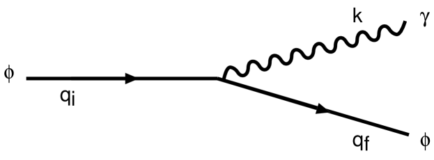
Figure 1: Feynman Diagram of the photon emission process

We follow a general prescription for interacting fields, based on the interaction picture approach (see e.g., [1, 2]). We focus on the radiation energy emitted through the process described by the Feynman diagram in Fig. 1. The S-matrix corresponding to the diagram is

$$S={-i\over\hbar}\int{{ieA^{\mu}\over\hbar}\left(\phi\partial_{\mu}\phi^{\dagger}-\phi^{\dagger}\partial_{\mu}\phi\right)}d^{4}x.$$ (2)

Here the field operator in the right-hand side, $A^{\mu}$ and $\phi$ obey the free field equations. The quantized free fields are expressed as follows. For the photon field, we have

$$A_{\mu}(x)=\sum_{r=1,2}\sum_{{\bm{k}}}\sqrt{\hbar\mu_{0}\over 2\omega(k)}\varepsilon_{\mu}^{(r)}\left\{\hat{a}_{\bm{k}}^{(r)}e^{-i\omega\eta}{e^{i{\bm{k}}\cdot{\bm{x}}}\over L^{3/2}}+{\rm Hermite~{}Conjugate}\right\},$$ (3)

where $\omega(k)=k$, $\varepsilon_{\mu}^{(r)}$ is the polarization vector, and $a_{\bm{k}}^{(r)}$ and $a_{\bm{k}}^{(r)}{}^{\dagger}$ are the annihilation and creation operators. They satisfies the commutation relations,

$$\left[\hat{a}_{\bm{k}}^{(r)},\hat{a}_{{\bm{k}}^{\prime}}^{(r^{\prime})}{}^{\dagger}\right]=\delta_{r,r^{\prime}}\delta_{{\bm{k}},{\bm{k}}^{\prime}},\hskip 28.45274pt\left[\hat{a}_{\bm{k}}^{(r)},\hat{a}_{{\bm{k}}^{\prime}}^{(r^{\prime})}\right]=\left[\hat{a}_{\bm{k}}^{(r)}{}^{\dagger},\hat{a}_{{\bm{k}}^{\prime}}^{(r^{\prime})}{}^{\dagger}\right]=0.$$

The vacuum state of the photon field is

$$\hat{a}_{\bm{k}}^{(r)}|0\big{>}^{(1)}=0,~{}\hskip 14.22636pt\mbox{for any}~{}{\bm{k}},~{}r.$$ (4)

The complex scalar field is quantized as

$$\phi(x)=\sqrt{\hbar}\sum_{{\bm{q}}}\left\{\hat{b}_{\bm{q}}\varphi_{\bm{q}}(\eta){e^{i{\bm{q}}\cdot{\bm{x}}}\over L^{3/2}}+\hat{c}_{\bm{q}}^{\dagger}\varphi_{\bm{q}}^{*}(\eta){e^{-i{\bm{q}}\cdot{\bm{x}}}\over L^{3/2}}\right\},$$ (5)

where $\hat{b}_{\bm{q}}$ and $\hat{b}_{\bm{q}}^{\dagger}$ satisfy

$$\left[\hat{b}_{{\bm{q}}},\hat{b}_{{\bm{q}}^{\prime}}^{\dagger}\right]=\delta_{{\bm{q}},{\bm{q}}^{\prime}},\hskip 28.45274pt\left[\hat{b}_{\bm{q}},\hat{b}_{{\bm{q}}^{\prime}}\right]=\left[\hat{b}_{\bm{q}}^{\dagger},\hat{b}_{{\bm{q}}^{\prime}}^{\dagger}\right]=0,$$ (6)

and $\hat{c}_{\bm{q}}$ and $\hat{c}_{\bm{q}}^{\dagger}$ satisfy the same commutation relations. The mode function $\varphi_{\bm{q}}(\eta)$ satisfies the equation of motion

$$\left({d^{2}\over d\eta^{2}}+{m^{2}a(\eta)^{2}\over\hbar^{2}}+{\bm{q}}^{2}\right)\varphi_{\bm{q}}(\eta)=0,$$ (7)

with the normalization condition

$${d\varphi_{\bm{q}}^{*}(\eta)\over d\eta}\varphi_{\bm{q}}(\eta)-\varphi_{\bm{q}}^{*}(\eta){d\varphi_{\bm{q}}(\eta)\over d\eta}=i.$$ (8)

The vacuum state of the complex scalar field is

$$\hat{b}_{\bm{q}}|0\big{>}^{(2)}=\hat{c}_{\bm{q}}|0\big{>}^{(2)}=0,~{}\hskip 14.22636pt{\rm for~{}any}~{}{\bm{q}}.$$ (9)

It may be noted that because of the time-variation of the mass $m\,a(\eta)$ the definition of the vacuum state can be ambiguous. In this section, however, we assume that there exists a natural stable vacuum state, which is the case when the WKB approximation is valid.

With the WKB approximation, the mode function $\varphi_{\bm{q}}(\eta)$ is given as

$$\varphi_{\bm{q}}(\eta)=\sqrt{1\over 2\Omega_{\bm{q}}(\eta)}\exp\left[-i\int_{\eta_{*}}^{\eta}{\Omega_{\bm{q}}(\eta^{\prime})}d\eta^{\prime}\right],$$ (10)

where

$$\Omega_{\bm{q}}(\eta)={\sqrt{m^{2}a(\eta)^{2}+\hbar^{2}{\bm{q}}^{2}}\over\hbar}.$$ (11)

We can write the condition that the WKB formula is valid, as (see e.g., [1])

$$\Omega_{{\bm{q}}}^{2}\gg{1\over 2}\Biggl{|}{\ddot{\Omega}_{\bm{q}}\over\Omega_{\bm{q}}}-{3\over 2}{\dot{\Omega}_{\bm{q}}^{2}\over\Omega_{\bm{q}}^{2}}\Biggr{|},$$ (12)

where the dot means the differentiation with respect to $\eta$.

Using the WKB mode functions, we evaluate the transition amplitude of the process described by Fig. 1,

$${\rm Transition~{}Amplitude}=\left<{\rm f}|S|{\rm i}\right>,$$ (13)

where the initial state and the final state are

$$|{\rm i}\big{>}=\hat{b}_{{\bm{q}}_{i}}^{\dagger}|0\big{>}^{(1)}|0\big{>}^{(2)},$$ (14)

$$|{\rm f}\big{>}=\hat{b}_{{\bm{q}}_{f}}^{\dagger}\hat{a}_{{\bm{k}}}^{(r)}{}^{\dagger}|0\big{>}^{(1)}|0\big{>}^{(2)},$$ (15)

respectively.

The radiation energy is

$$E={(2\pi)^{3}\over L^{3}}\sum_{r=1,2}\sum_{\bm{k}}\sum_{\bm{q}}\hbar\omega(k)|\rm Transition~{}Amplitude|^{2},$$ (16)

which gives

$$E={2{e^{2}}\over\varepsilon_{0}}\int{d^{3}{\bm{k}}\over(2\pi)^{3}}\left({\bm{q}}_{i}^{2}-{({\bm{q}}_{i}\cdot{\bm{k}})^{2}\over k^{2}}\right)\left|\int d\eta e^{ik\eta}\varphi_{{\bm{q}}_{f}}^{*}(\eta)\varphi_{{\bm{q}}_{i}}(\eta)\right|^{2},$$ (17)

where ${\bm{q}}_{f}={\bm{q}}_{i}-{\bm{k}}$, and $\varepsilon_{0}$ is the permittivity of vacuum, which is related to $\mu_{0}$ as $\varepsilon_{0}\mu_{0}=1/c^{2}=1$. We set ${\bm{q}}_{i}\cdot{\bm{k}}=q_{i}k\cos\theta$, and rewrite (17) as

$$E={e^{2}\over 2\varepsilon_{0}}\int{d^{3}{\bm{k}}\over(2\pi)^{3}}{\bm{q}}_{i}^{2}\left(1-\cos^{2}\theta\right)$$

$$\times\left|\int d\eta{1\over\sqrt{\Omega_{{\bm{q}}_{i}}(\eta)\Omega_{{\bm{q}}_{f}}(\eta)}}\exp\left[ik\eta+i\int_{\eta_{*}}^{\eta}d\eta^{\prime}\Omega_{{\bm{q}}_{f}}(\eta^{\prime})-i\int_{\eta_{*}}^{\eta}d\eta^{\prime}\Omega_{{\bm{q}}_{i}}(\eta^{\prime})\right]\right|^{2},$$

where

$$p^{0}=\hbar\Omega_{\bm{q}}(\eta)=\sqrt{\hbar^{2}{\bm{q}}^{2}+m^{2}a(\eta)^{2}}=\sqrt{{\bm{p}}^{2}+m^{2}a(\eta)^{2}},$$ (19)

where the first and last equalities follow from the definition of the momentum of the charged particle,

$${\bm{p}}=\hbar{\bm{q}}.$$ (20)

We follow the prescription in ref. [8],

$$\int_{\eta_{*}}^{\eta}d\eta^{\prime}\left(\Omega_{{\bm{p}}_{f}}(\eta^{\prime})-\Omega_{{\bm{q}}_{i}}(\eta^{\prime})\right) \simeq \int_{\eta_{*}}^{\eta}d\eta^{\prime}\left({\bm{q}}_{f}-{\bm{q}}_{i}\right)\cdot{\partial\over\partial{\bm{q}}}\sqrt{{\bm{q}}^{2}+{m^{2}a(t)^{2}\over\hbar^{2}}}\Bigg{|}_{{\bm{p}}={\bm{p}}_{i}}$$

$$= -\int_{\eta_{*}}^{\eta}d\eta^{\prime}{{\bm{k}}\cdot{\bm{p}}_{i}\over p^{0}},$$

and

$$\sqrt{\Omega_{{\bm{q}}_{i}}(\eta)\Omega_{{\bm{q}}_{f}}(\eta)}\simeq\Omega_{{\bm{q}}_{i}}(\eta)={p^{0}\over\hbar},$$ (22)

where we used ${\bm{q}}_{f}={\bm{q}}_{i}-{\bm{k}}$ and

$$k(=|{\bm{k}}|)\ll q_{f}(=|{\bm{q}}_{f}|),~{}~{}{\rm and}~{}q_{i}(=|{\bm{q}}_{i}|).$$ (23)

Then, we have

$$E = {e^{2}\over 2\varepsilon_{0}}\int_{0}^{\infty}{dkk^{2}\over(2\pi)^{2}}\int_{-1}^{1}d\cos\theta\left(1-\cos^{2}\theta\right)$$ (24)

$$\times\left|\int d\eta{p_{i}\over p^{0}(\eta)}\exp\left[ik\int_{\eta_{*}}^{\eta}d\eta^{\prime}\left(1-{p_{i}\cos\theta\over p^{0}(\eta^{\prime})}\right)\right]\right|^{2}.$$

We can choose ${{\bm{p}}}_{i}$ to be in proportion to $z$-axis. Therefore, we may write

$$p_{i}=p^{z}={dz\over d\tau},\qquad p^{0}={d\eta\over d\tau},$$ (25)

where $\tau$ is the parameter chosen as

$$\eta_{\mu\nu}{dx^{\mu}\over d\tau}{dx^{\nu}\over d\tau}=-(p^{0})^{2}+p_{z}^{2}=-m^{2}a^{2}(\eta).$$ (26)

Because we may write $p_{i}/p^{0}=dz/d\eta$, we have

$$\left|\int d\eta{p_{i}\over p^{0}(\eta)}\exp\left[i\int_{\eta_{*}}^{\eta}d\eta^{\prime}k\left(1-{p_{i}\cos\theta\over p^{0}(\eta^{\prime})}\right)\right]\right|^{2}$$

$$~{}~{}~{}~{}~{}~{}~{}~{}~{}~{}~{}~{}~{}~{}~{}~{}~{}~{}=\left|\int dz\exp\left[ik(\eta(z)-\cos\theta z)\right]\right|^{2}.$$ (27)

Instead of $z$ or $\eta$, introducing the variable $\xi$ defined by

$$\xi\equiv\eta-\cos\theta z(\eta),$$ (28)

we have

$$E={e^{2}\over 2\varepsilon_{0}}\int_{0}^{\infty}{dkk^{2}\over(2\pi)^{2}}\int_{-1}^{1}d\cos\theta\left(1-\cos^{2}\theta\right)\left|\int d\xi{dz\over d\xi}e^{ik\xi}\right|^{2}.$$ (29)

Furthermore, the partial integration gives

$$\Biggl{|}\int d\xi{dz\over d\xi}e^{ik\xi}\Biggr{|}^{2}={1\over k^{2}}\Biggl{|}\int d\xi{d^{2}z\over d\xi^{2}}e^{ik\xi}\Biggr{|}^{2},$$ (30)

where we have assumed that the boundary term has no contribution. The neglect of the boundary term is justified if $|dz/d\xi|$ is finite at all times. Since we have

$$\frac{dz}{d\xi}=\frac{\dot{z}}{1-\cos\theta\dot{z}}\,;\quad|\dot{z}|=\frac{|p_{z}|}{\sqrt{p_{z}^{2}+m^{2}a^{2}}}<1\,,$$ (31)

where $\dot{z}=dz/d\eta$, we see that $|dz/d\xi|$ is bounded at all times.

The integration with respect to $k$ yields

$$E={e^{2}\over 8\pi\varepsilon_{0}}\int_{-1}^{1}d\cos\theta(1-\cos^{2}\theta)\int d\xi\Biggl{(}{d^{2}z\over d\xi^{2}}\Biggr{)}^{2},$$ (32)

where the integration is extended to $-\infty\leq k\leq\infty$, and divided by the factor 2 [8]. From the definition of $\xi$, we have

$${d\xi\over d\eta}=(1-\dot{z}\cos\theta),~{}~{}~{}~{}~{}~{}{d^{2}z\over d\xi^{2}}={\ddot{z}\over(1-\dot{z}\cos\theta)^{3}}\,.$$ (33)

Then, Eq. (32) is rephrased as

$$E={e^{2}\over 8\pi\varepsilon_{0}}\int_{-1}^{1}d\cos\theta(1-\cos^{2}\theta)\int d\eta{\ddot{z}^{2}\over(1-\dot{z}\cos\theta)^{5}}.$$ (34)

Finally, the integration with respect to $\cos\theta$ yields

$$E={e^{2}\over 6\pi\varepsilon_{0}}\int d\eta{\ddot{z}^{2}\over(1-\dot{z}^{2})^{3}}.$$ (35)

This result is the same as the Larmor formula in the case when the particle moves along a straight line [7]. In the present case, Eq. (35) is rewritten as

$$E={e^{2}p_{i}^{2}\over 6\pi\varepsilon_{0}m^{2}}\int d\eta{\dot{a}^{2}\over a^{4}}.$$ (36)

Note that this is the energy in the conformally rescaled spacetime, which is not the physical energy. From this expression, however, we can read the physical radiation energy as ${\cal E}=E/a$, and the physical rate of the radiation energy per unit time as

$${d{\cal{E}}\over dt}={1\over a^{2}}{dE\over d\eta}={e^{2}p_{phys}^{2}H^{2}\over 6\pi\varepsilon_{0}m^{2}},$$ (37)

where $t$ is the cosmic time, $p_{phys}(=p_{i}/a)$ is the physical momentum and $H$ is the Hubble expansion rate. This result is consistent with that in ref. [5], which is obtained from consideration of the classical electromagnetic radiation formula of a moving charge in an expanding universe.

Finally in this section, let us summarize the necessary condition for reproducing the radiation formula in the classical electromagnetic theory. We started with the WKB formula of the mode function, for which Eq. (12) is needed. In addition, we assumed Eq. (23). Although this condition is independent of the necessary condition for the WKB approximation, Eq. (12), we assumed it because this additional assumption is necessary to recover the conventional picture for the classical radiation from a charged massive particle, in which the massive field should behave like a particle and the photon field should behave like a wave.

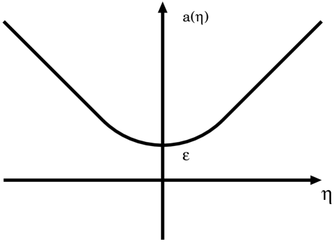
Figure 2: The scale factor of the bounced radiation dominant universe as a function $\eta$.

3 Quantum radiation formula

In this section, we calculate the radiated energy without the WKB approximation. We start with reviewing the formalism. Now we return to the S-matrix expression (2). A characteristic feature of the quantum field theory in curved spacetime is that vacuum state may not be stable. Namely, the vacuum state may change, and the particle creation phenomenon can occur. This vacuum effect is not taken into account in the analysis based on the WKB approximation in the previous section. In this section, we adopt the formalism for evaluating the S-matrix element, taking the vacuum effect into account.

For definiteness, we assume that the interaction is switched off in the asymptotic past infinity ($\eta=-\infty$) and future infinity ($\eta=+\infty$), where the different vacuum states $|0\big{>}_{\rm in}^{(2)}$ and $|0\big{>}_{\rm out}^{(2)}$, respectively, are defined for the free field. Then, similar to Eq. (5), we may write the quantized field as

$$\phi(x)=\sqrt{\hbar}\sum_{{\bm{q}}}\left\{\hat{b}^{\rm in}_{\bm{q}}\varphi^{\rm in}_{\bm{q}}(\eta){e^{i{\bm{q}}\cdot{\bm{x}}}\over L^{3/2}}+\hat{c}^{\rm in}_{\bm{q}}{}^{\dagger}\varphi^{\rm in}_{\bm{q}}{}^{*}(\eta){e^{-i{\bm{q}}\cdot{\bm{x}}}\over L^{3/2}}\right\},$$ (38)

or as

$$\phi(x)=\sqrt{\hbar}\sum_{{\bm{q}}}\left\{\hat{b}^{\rm out}_{\bm{q}}\varphi^{\rm out}_{\bm{q}}(\eta){e^{i{\bm{q}}\cdot{\bm{x}}}\over L^{3/2}}+\hat{c}^{\rm out}_{\bm{q}}{}^{\dagger}\varphi^{\rm out}_{\bm{q}}{}^{*}(\eta){e^{-i{\bm{q}}\cdot{\bm{x}}}\over L^{3/2}}\right\},$$ (39)

where $b^{\rm in}_{\bm{q}}$, $c^{\rm in}_{\bm{q}}$ and $b^{\rm in}{}^{\dagger}_{\bm{q}}$, $c^{\rm in}{}^{\dagger}_{\bm{q}}$ are the annihilation and the creation operators, respectively, with respect to the in-vacuum at $\eta=-\infty$, while $b^{\rm out}_{\bm{q}}$, $c^{\rm out}_{\bm{q}}$ and $b^{\rm out}{}^{\dagger}_{\bm{q}}$, $c^{\rm out}{}^{\dagger}_{\bm{q}}$ are those with respect to the out-vacuum at $\eta=+\infty$. The in-vacuum and out-vacuum states are expressed as

$${\hat{b}^{\rm in}_{\bm{q}}}|0\big{>}_{\rm in}^{(2)}={\hat{c}^{\rm in}_{\bm{q}}}|0\big{>}_{\rm in}^{(2)}=0,$$ (40)

and

$${\hat{b}^{\rm out}_{\bm{q}}}|0\big{>}_{\rm out}^{(2)}={\hat{c}^{\rm out}_{\bm{q}}}|0\big{>}_{\rm out}^{(2)}=0,$$ (41)

for any ${\bm{q}}$. These annihilation and the creation operators satisfy the same commutation relations as Eq. (6).

In Eqs. (38) and (39), $\varphi_{\bm{q}}^{\rm in}(\eta)$ and $\varphi_{\bm{q}}^{\rm out}(\eta)$ are the mode functions with respect to the vacuum states $|0\big{>}_{\rm in}^{(2)}$ and $|0\big{>}_{\rm out}^{(2)}$, respectively. They are related by the Bogoliubov transformation,

$$\varphi_{\bm{q}}^{\rm in}(\eta)=\alpha_{\bm{q}}\varphi_{\bm{q}}^{\rm out}(\eta)+\beta_{\bm{q}}\varphi_{\bm{q}}^{\rm out}{}^{*}(\eta)$$ (42)

where $\alpha_{\bm{q}}$ and $\beta_{\bm{q}}$ satisfy the normalization condition

$$|\alpha_{\bm{q}}|^{2}-|\beta_{\bm{q}}|^{2}=1.$$ (43)

The creation and annihilation operators are related as

$$\hat{b}^{\rm in}_{\bm{q}}=\alpha_{\bm{q}}^{*}\hat{b}^{\rm out}_{\bm{q}}-\beta_{\bm{q}}^{*}\hat{c}^{\rm out}_{-{\bm{q}}}{}^{\dagger},$$ (44)

$$\hat{c}^{\rm in}_{-{\bm{q}}}{}^{\dagger}=\alpha_{\bm{q}}\hat{c}^{\rm out}_{-{\bm{q}}}{}^{\dagger}-\beta_{\bm{q}}\hat{b}^{\rm out}_{{\bm{q}}}.$$ (45)

Using the above relations, we have

$$\varphi_{\bm{q}}^{\rm out}{}^{*}(\eta)\hat{b}^{\rm out}_{\bm{q}}{}^{\dagger}+\varphi_{\bm{q}}^{\rm out}{}(\eta)\hat{c}^{\rm out}_{-{\bm{q}}}={\varphi_{\bm{q}}^{\rm in}{}^{*}(\eta)\over\alpha_{\bm{q}}^{*}}\hat{b}^{\rm out}_{\bm{q}}{}^{\dagger}+{\varphi_{\bm{q}}^{\rm out}(\eta)\over\alpha_{\bm{q}}^{*}}\hat{c}^{\rm in}_{-{\bm{q}}}$$ (46)

and

$$\varphi_{\bm{q}}^{\rm in}{}(\eta)\hat{b}^{\rm in}_{\bm{q}}{}+\varphi_{\bm{q}}^{\rm in}{}^{*}(\eta)\hat{c}^{\rm in}_{-{\bm{q}}}{}^{\dagger}={\varphi_{\bm{q}}^{\rm out}{}(\eta)\over\alpha_{\bm{q}}^{*}}\hat{b}^{\rm in}_{\bm{q}}{}+{\varphi_{\bm{q}}^{\rm in}{}^{*}(\eta)\over\alpha_{\bm{q}}^{*}}\hat{c}^{\rm out}_{-{\bm{q}}}{}^{\dagger}.$$ (47)

As for the photon field, because of its conformal invariance, the vacuum state is invariant in time, $|0\big{>}^{(1)}=|0\big{>}^{(1)}_{\rm in}=|0\big{>}^{(1)}_{\rm out}$.

The transition amplitude in the lowest order of $e$ is evaluated in the similar form as Eq. (13), but with

$$|{\rm i}\big{>}_{\rm in}=\hat{b}_{{\bm{q}}_{i}}^{\rm in}{}^{\dagger}|0\big{>}^{(1)}|0\big{>}^{(2)}_{\rm in},$$ (48)

$$|{\rm f}\big{>}_{\rm out}=\hat{b}_{{\bm{q}}_{f}}^{\rm out}{}^{\dagger}\hat{a}_{{\bm{k}}}^{(r)}{}^{\dagger}|0\big{>}^{(1)}|0\big{>}^{(2)}_{\rm out}.$$ (49)

In the computation of the transition amplitude, it is necessary to regularize the divergence arising from the vacuum-to-vacuum amplitude. In the flat background, this can be done unambiguously by taking the normal-order product of operators. However, in a curved spacetime, there arises ambiguity because the in-state annihilation/creation operators are different from the out-state annihilation/creation operators. In fact, there will be particle creation from vacuum and the vacuum-to-vacuum amplitude will not longer be unity any more.

To deal with this situation properly, we consider the generalized normal product of operators, which is defined as the form where the operators are expressed only in terms of the in-state annihilation operator and the out-state creation operators, and all the out-state creation operator are placed to the left of all the in-state annihilation operators [9]. This is adopted in ref. [3]. The nice properties of this generalized normal ordering are that it is symmetrically defined with respect to the in-state and out-state operators, and that the vacuum-to-vacuum amplitude is normalized to unity. In particular, this latter property means that it minimizes the effect of particle creation from vacuum. Since what we are interested in is not the vacuum particle creation but the transition amplitude for a massive particle to radiate under the electromagnetic interaction, we adopt the generalized normal ordering to regularize the divergence. We note that what would be actually observed will be inevitably contaminated by the effect of particle creation. However, whether there is a way to separate out this vacuum effect observationally is beyond the scope of the present paper.

Following ref.[3], we define

$${\rm Transition~{}amplitude}={\displaystyle{{}_{\rm out}\bigl{<}{\rm f}|N[S]|{\rm i}\big{>}_{\rm in}}\over\displaystyle{{}_{\rm out}\bigl{<}0|0\big{>}_{\rm in}}}.$$ (50)

Here $|0\big{>}_{\rm in}=|0\big{>}^{(1)}|0\big{>}^{(2)}_{\rm in}$ and $|0\big{>}_{\rm out}=|0\big{>}^{(1)}|0\big{>}^{(2)}_{\rm out}$, respectively, $N[S]$ denotes the generalized normal product of the S-matrix, and ${}_{\rm out}\bigl{<}0|0\bigr{>}_{\rm in}$ is the vacuum to vacuum amplitude.

We then find the formula for the radiation energy as

$$E={2e^{2}{{{\bm{q}}}_{i}}^{2}\over(2\pi)^{2}\varepsilon_{0}}\int_{0}^{\infty}dkk^{2}\int_{-1}^{1}d\cos\theta{1-\cos^{2}\theta\over|\alpha_{{{\bm{q}}}_{i}}|^{2}|\alpha_{{{\bm{q}}}_{f}}|^{2}}\Biggl{|}\int d\eta e^{ik\eta}\varphi^{in*}_{{{\bm{q}}}_{f}}\varphi^{\rm out}_{{{\bm{q}}}_{i}}\Biggr{|}^{2}.$$ (51)

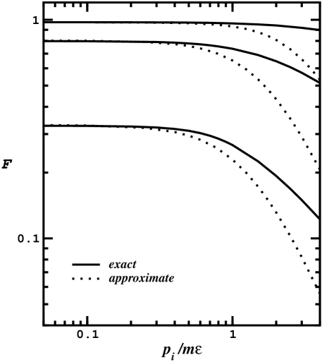
Figure 3: $F$ as function of $p_{i}/m\epsilon$ with fixed as $\hbar{\varrho}/m\epsilon^{2}=0.01,~{}0.1,~{}1$, from top to bottom. The solid curve is exact, Eq. (66), while the dotted curve is approximate, Eq. (68).

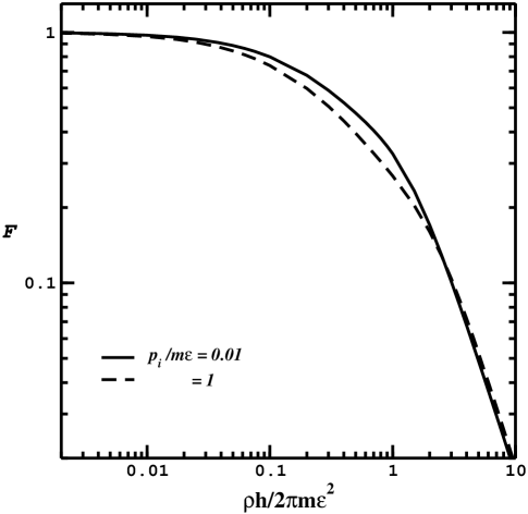
Figure 4: $F$ as function of $\hbar{\varrho}/m\epsilon^{2}$ with fixed as $p_{i}/m\epsilon=0.01$(dashed curve) and $1$(solid curve).

3.1 Example I

In this subsection, we consider a time-symmetric bounce universe which asymptotically approaches a contracting and expanding radiation-dominated universe (see Fig. 2). The scale factor is given in terms of the conformal time $\eta$ by [10, 11]

$$a(\eta)=\sqrt{{\varrho}^{2}\eta^{2}+\epsilon^{2}}\qquad(-\infty<\eta<\infty),$$ (52)

which recovers a radiation-dominated Friedmann universe in the asymptotic regions, $a(t)\propto t^{1/2}~{}(\eta\rightarrow\pm\infty)$. In this background spacetime, the WKB formula (35) gives

$$E_{cl}={e^{2}p_{i}^{2}\over 6\pi\varepsilon_{0}m^{2}}\int\nolimits_{-\infty}^{\infty}d\eta{{\varrho}^{4}\eta^{2}\over({\varrho}^{2}\eta^{2}+\epsilon^{2})^{3}}={e^{2}p_{i}^{2}{\varrho}\over 48\varepsilon_{0}m^{2}\epsilon^{3}}.$$ (53)

Equation of motion (7) is reduced to the Weber’s differential equation

$${d^{2}\varphi\over dz^{2}}+\Bigl{(}\nu+{1\over 2}-{1\over 4}z^{2}\Bigr{)}\varphi=0,$$ (54)

where

$$\nu={1\over 2}\Bigl{(}{{{\bm{q}}}^{2}+m^{2}\epsilon^{2}/\hbar^{2}\over\pm im{\varrho}/\hbar}-1\Bigr{)},\qquad z=\pm(1\pm i)\sqrt{m{\varrho}/\hbar}\eta.$$ (55)

Therefore, the mode functions are constructed as [12]

$$\varphi^{\rm in}_{{{\bm{q}}}}(\eta)={1\over(2m{\varrho}/\hbar)^{1/4}}e^{-\pi\lambda/4}D_{i\lambda-1/2}(-(1-i)\sqrt{m{\varrho}/\hbar}\eta),$$ (56)

$$\varphi^{\rm out}_{{{\bm{q}}}}(\eta)={1\over(2m{\varrho}/\hbar)^{1/4}}e^{-\pi\lambda/4}D_{-i\lambda-1/2}((1+i)\sqrt{m{\varrho}/\hbar}\eta),$$ (57)

with

$$\lambda={{{\bm{q}}}^{2}+m^{2}\epsilon^{2}/\hbar^{2}\over 2m{\varrho}/\hbar}.$$ (58)

Using the mathematical formula for the parabolic cylinder function,

$$D_{\nu}(z)={\sqrt{2\pi}\over\Gamma(-\nu)}e^{\pm i\pi(\nu+1)/2}D_{-\nu-1}(\mp iz)+e^{\pm i\pi\nu}D_{\nu}(-z).$$ (59)

we easily find the Bogoliubov coefficients

$$\alpha_{{\bm{q}}}={\sqrt{2\pi}\over\Gamma(-i\lambda+1/2)}e^{\pi(-\lambda+i/2)/2},\qquad\beta_{{\bm{q}}}=e^{\pi(-\lambda-i/2)}.$$ (60)

Using the mathematical formula for the parabolic cylinder function [13],

$$\int\nolimits_{-\infty}^{\infty}d\xi e^{-i\rho\xi}D_{-i\beta}((1+i)\xi)D_{-i\alpha}(-(1+i)\xi)$$

$$=\sqrt{\pi}\exp\Bigl{[}-{\pi\over 4}i+{3\pi\over 4}(\alpha-\beta)+{i\over 4}\rho^{2}+i(\alpha-\beta)\ln{\rho\over\sqrt{2}}\Bigr{]}$$

$$\times U\Bigl{(}i\alpha,1+i(\alpha-\beta),-i{\rho^{2}\over 2}\Bigr{)},$$ (61)

we have

$$\int\nolimits_{-\infty}^{\infty}d\eta e^{ik\eta}\varphi_{{{\bm{p}}}_{i}}^{\rm out}(\eta)\varphi_{{{\bm{p}}}_{f}}^{\rm in*}(\eta)$$

$$={\sqrt{\pi}\hbar\over\sqrt{2}m{\varrho}}e^{-\pi(\lambda+\bar{\lambda})/4}\exp\Bigl{[}-{\pi\over 4}i+{3\pi\over 4}(\lambda-\bar{\lambda})+{i\over 4}{k^{2}\over m{\varrho}/\hbar}+i(\lambda-\bar{\lambda})\ln{k\over\sqrt{2m{\varrho}/\hbar}}\Bigr{]}$$

$$\hskip 113.81102pt\times U\Bigl{(}i\lambda+{1\over 2},1+(\lambda-\bar{\lambda}),-i{k^{2}\over 2m{\varrho}/\hbar}\Bigr{)},$$ (62)

where $U(a,c,z)$ is the second order confluent hypergeometric function [14], and we used the notation

$$\lambda = {{{\bm{q}}_{i}}^{2}+m^{2}\epsilon^{2}/\hbar^{2}\over 2m{\varrho}/\hbar}={1\over 2}{m\epsilon^{2}\over{\varrho}\hbar}\left(1+{{{\bm{p}}}_{i}^{2}\over m^{2}\epsilon^{2}}\right),$$ (63)

$$\bar{\lambda} = {{({\bm{q}}_{i}-k)}^{2}+m^{2}\epsilon^{2}/\hbar^{2}\over 2m{\varrho}/\hbar}={1\over 2}{m\epsilon^{2}\over{\varrho}\hbar}\left(1+{({{\bm{p}}}_{i}-\hbar{{\bm{k}}})^{2}\over m^{2}\epsilon^{2}}\right)$$

$$= {1\over 2}{m\epsilon^{2}\over{\varrho}\hbar}\left(1+{{{\bm{p}}}_{i}^{2}\over m^{2}\epsilon^{2}}-2{{p}_{i}\over m\epsilon}{\hbar{\varrho}\over m\epsilon^{2}}\hat{k}\cos\theta+{\hbar^{2}{\varrho}^{2}\over m^{2}\epsilon^{4}}\hat{k}^{2}\right).$$

Then, the radiation energy $E$ is represented by

$$E=E_{cl}\times F\Bigl{(}{p_{i}\over\epsilon m},{\hbar{\varrho}\over\epsilon^{2}m}\Bigr{)},$$ (65)

where

$$F\Bigl{(}{p_{i}\over\epsilon m},{\hbar{\varrho}\over\epsilon^{2}m}\Bigr{)}={12\over\pi}\int\nolimits_{0}^{\infty}d\hat{k}\hat{k}^{2}\int\nolimits_{-1}^{1}d\cos\theta{1-\cos^{2}\theta\over(1-e^{-2\pi\lambda})(1-e^{-2\pi\bar{\lambda}})}e^{\pi(\lambda-2\bar{\lambda})}$$

$$\hskip 142.26378pt\times\Bigl{|}U\Bigl{(}i\lambda+{1\over 2},1+i(\lambda-\bar{\lambda}),-i{\hbar{\varrho}\hat{k}^{2}\over 2m\epsilon^{2}}\Bigr{)}\Bigr{|}^{2},$$ (66)

and we have defined $\hat{k}=(\epsilon/{\varrho}){k}$. Note that the function $F$ describes the deviation from the WKB formula.

Now let us consider the classical limit by taking the limit $\hbar\rightarrow 0$. We use the mathematical formula

$$\lim_{a\to\infty}U(a,c,z/a)={2z^{(1-c)/2}K_{c-1}(2\sqrt{z})\over\Gamma(a+1-c)},$$ (67)

where $K_{\nu}(z)$ is the modified Bessel function. Then, we have

$$F\Bigl{(}{p_{i}\over m\epsilon},{\hbar{\varrho}\over m\epsilon^{2}}\Bigr{)} \simeq {24\over\pi^{2}}\int\nolimits_{0}^{\infty}d\hat{k}\hat{k}^{2}\int\nolimits_{-1}^{1}dx(1-x^{2})e^{\pi(\lambda-\bar{\lambda})}$$ (68)

$$\times\Biggl{|}K_{i(\lambda-\bar{\lambda})}\Biggl{(}\hat{k}\sqrt{1+{p_{i}^{2}\over m^{2}\epsilon^{2}}}\Biggr{)}\Biggr{|}^{2}$$

with

$$\lambda-\bar{\lambda}={p_{i}\over m\epsilon}\hat{k}x-{1\over 2}{\hbar{\varrho}\over m\epsilon^{2}}\hat{k}^{2}.$$ (69)

We have evaluated the function $F$ numerically. The cases of $p_{i}/m\epsilon=0.01$ and $1$ are shown in Fig. 4. In all cases we analyzed, we found $F$ is a decreasing function of $\hbar\varrho/m\epsilon^{2}$.

In the limit $\hbar\rightarrow 0$,

$$\lambda-\bar{\lambda}={p_{i}\over m\epsilon}\hat{k}x=s\,.$$ (70)

Then, we have

$$\lim_{\hbar\rightarrow 0}F={24\over\pi^{2}}\int\nolimits_{0}^{\infty}d\hat{k}\hat{k}^{2}\int\nolimits_{-1}^{1}dx(1-x^{2})e^{\pi s}\Biggl{|}K_{is}\Biggl{(}\hat{k}\sqrt{1+{p_{i}^{2}\over m^{2}\epsilon^{2}}}\Biggr{)}\Biggr{|}^{2}.$$ (71)

Thus $F$ is the function of only $p_{i}/m\epsilon$ in this limit. By numerical analysis of the right-hand side of Eq. (71), we find

$$\lim_{\hbar\rightarrow 0}F=1,$$ (72)

irrespectively of $p_{i}/m\epsilon$. We therefore infer that the integral of Eq. (71) gives $1$. Although we have not yet succeeded to show it in general, we can show that, for the case $p_{i}/m\epsilon\ll 1$, Eq. (71) yields

$$\lim_{\hbar\rightarrow 0}F\simeq{24\over\pi^{2}}\int\nolimits_{-1}^{1}dx(1-x^{2})\int\nolimits_{0}^{\infty}d\hat{k}\hat{k}^{2}K_{0}(\hat{k})^{2}=1,$$ (73)

by using the integral formula for the modified Bessel function [14],

$$\int\nolimits_{0}^{\infty}x^{-\lambda}K_{\mu}(ax)K_{\nu}(bx)dx$$

$$={2^{-2-\lambda}a^{-nu+\lambda-1}b^{\nu}\over\Gamma(1-\lambda)}\Gamma\Bigl{(}{1-\lambda+\mu+\nu\over 2}\Bigr{)}\Gamma\Bigl{(}{1-\lambda-\mu+\nu\over 2}\Bigr{)}$$

$$\hskip 85.35826pt\times\Gamma\Bigl{(}{1-\lambda+\mu-\nu\over 2}\Bigr{)}\Gamma\Bigl{(}{1-\lambda-\mu-\nu\over 2}\Bigr{)}$$

$$\hskip 85.35826pt\times F\Bigl{(}{1-\lambda+\mu+\nu\over 2},{1-\lambda-\mu+\nu\over 2};1-\lambda;1-{b^{2}\over a^{2}}\Bigr{)}.$$ (74)

This demonstrates that the exact formula in the limit of ${\hbar\rightarrow 0}$ agrees with the WKB approximate formula. Then, the decrease of $F$ from $1$ comes from the term in proportion to $\hbar$, hence the suppression is understood as the quantum effect.

Let us summarize the result. The quantum radiation formula agrees with the WKB formula under the condition

$$\lambda={1\over 2}{m\epsilon^{2}\over{\varrho}\hbar}\left(1+{{{\bm{p}}}_{i}^{2}\over m^{2}\epsilon^{2}}\right)\gg 1,$$ (75)

$${p_{i}\over m\epsilon}\hat{k}\gg{1\over 2}{\hbar{\varrho}\over m\epsilon^{2}}\hat{k}^{2}.$$ (76)

We can show that the former condition (75) is derived from the condition for the WKB approximation, Eq.(12), while the latter condition (76) is equivalent to $p_{i}\gg\hbar k$, i.e., Eq.(23). The former condition is satisfied when the Compton wavelength of the charged particle is shorter than the Hubble horizon length around the bounce regime defined by $a\sim\epsilon\sim{\varrho}\eta$ (see below), where the classical radiation rate becomes maximum. Figure 3 plots $F$ as a function of $p_{i}/m\epsilon$ with fixed as $\hbar{\varrho}/m\epsilon^{2}=1$, 0.1 and 0.01. Figure 4 plots $F$ as a function of $\hbar{\varrho}/m\epsilon^{2}$ with fixed as $p_{i}/m\epsilon=0.01$ and $1$. These figures show $F=1$ for $p_{i}/m\epsilon\lower 2.15277pt\hbox{$\;\buildrel<\over{\sim}\;$}1$ and $\hbar{\varrho}/m\epsilon^{2}\ll 1$, and the suppression $F<1$ for the other region.

Finally in this section, we mention the physical meaning of these parameters. Around the bounce regime $a\sim\epsilon\sim{\varrho}\eta$, we can write

$${p_{i}\over m\epsilon}\simeq{p_{phys}\over m}\Big{|}_{\rm bounce},\qquad{\hbar{\varrho}\over m\epsilon^{2}}\simeq\lambda_{\rm C}{H}\Big{|}_{\rm bounce},$$ (77)

where $p_{phys}=p_{i}/\epsilon$ is the physical momentum, $\lambda_{\rm C}=\hbar/m$ is the Compton wavelength, and $H|_{\rm bounce}={\varrho}/\epsilon^{2}$ is the Hubble expansion rate, respectively. Thus $p_{i}/m\epsilon$ is the relativistic factor, and $\hbar{\varrho}/m\epsilon^{2}$ can be regarded as the the ratio of the Hubble horizon length to the Compton wavelength of the charged particle, around the bouncing regime.

3.2 Example II

Here we consider a Friedmann spacetime with the scale factor

$$a=\left\{\begin{array}[]{cc}+\bar{t}+\epsilon&({\bar{t}}>0)\\ -\bar{t}+\epsilon&({\bar{t}}<0)\end{array}\right.=\left\{\begin{array}[]{cc}\epsilon e^{+{\bar{\eta}}}&({\bar{\eta}}>0)\\ \epsilon e^{-{\bar{\eta}}}&({\bar{\eta}}<0)\end{array}\right.,$$ (82)

where $\epsilon(>0)$ is a small constant, ${\bar{t}}=t/t_{0}$ and ${\bar{\eta}}=\eta/\eta_{0}$. This mimics a Milne-like bounce universe but with a flat spatial geometry.

The solution of the Klein-Gordon equation is written with the Bessel function, and the positive frequency mode function is [15]

$$\varphi_{q}=N_{\bar{q}}\times\left\{\begin{array}[]{lc}H_{-i{\bar{q}}}^{(2)}({\bar{m}}(+{\bar{t}}+\epsilon))&(t>0)\\ H_{i{\bar{q}}}^{(1)}({\bar{m}}(-{\bar{t}}+\epsilon))&(t<0)\end{array}\right.,$$ (85)

where

$$N_{\bar{q}}=e^{-{\bar{q}}\pi/2}{\sqrt{\eta_{0}\pi}\over 2}$$ (86)

from the normalization condition, and we have defined ${\bar{m}}=\eta_{0}m/\hbar$ and ${\bar{q}}=\eta_{0}q$.

The in- and out-vacuum mode functions are therefore given by

$$\varphi^{\rm in}_{q} = N_{\bar{q}}\times\left\{\begin{array}[]{lc}\alpha_{\bar{q}}H_{-i{\bar{q}}}^{(2)}({\bar{m}}({\bar{t}}+\epsilon))+\beta_{\bar{q}}H_{i{\bar{q}}}^{(1)}({\bar{m}}({\bar{t}}+\epsilon))&\hskip 28.45274pt({\bar{t}}>0)\\ H_{i{\bar{q}}}^{(1)}({\bar{m}}(-{\bar{t}}+\epsilon)))&\hskip 28.45274pt({\bar{t}}<0)\end{array}\right.$$ (89)

$$\varphi^{\rm out}_{q} = N_{\bar{q}}\times\left\{\begin{array}[]{lc}H_{-i{\bar{q}}}^{(2)}({\bar{m}}({\bar{t}}+\epsilon)))&\hskip 28.45274pt({\bar{t}}>0)\\ \bar{\alpha}_{\bar{q}}H_{i{\bar{q}}}^{(1)}({\bar{m}}(-{\bar{t}}+\epsilon))+\bar{\beta}_{\bar{q}}H_{-i{\bar{q}}}^{(2)}({\bar{m}}(-{\bar{t}}+\epsilon))&\hskip 28.45274pt({\bar{t}}<0)\end{array}\right.,$$ (92)

where the coefficients are

$$\alpha_{\bar{q}}={\pi{\bar{m}}\epsilon\over 4i}e^{-\pi{\bar{q}}}(H_{i{\bar{q}}}^{(1)}({\bar{m}}\epsilon))^{2}{{}^{\prime}},$$

$$\beta_{\bar{q}}=-{\pi{\bar{m}}\epsilon\over 4i}e^{-\pi{\bar{q}}}(H_{i{\bar{q}}}^{(1)}({\bar{m}}\epsilon)H_{-i{\bar{q}}}^{(2)}({\bar{m}}\epsilon))^{\prime},$$

$$\bar{\alpha}_{\bar{q}}=-{\pi{\bar{m}}\epsilon\over 4i}e^{-\pi{\bar{q}}}(H_{-i{\bar{q}}}^{(2)}({\bar{m}}\epsilon)){}^{2}{}^{\prime}=\alpha_{\bar{q}}^{*},$$

$$\bar{\beta}_{\bar{q}}={\pi{\bar{m}}\epsilon\over 4i}e^{-\pi{\bar{q}}}(H_{i{\bar{q}}}^{(1)}({\bar{m}}\epsilon)H_{-i{\bar{q}}}^{(2)}({\bar{m}}\epsilon))^{\prime}=\beta_{{\bar{q}}}^{*},$$ (94)

and the prime means $H(z)^{\prime}=dH(z)/dz$.

We may write

$$e^{i{\bar{k}}{\bar{\eta}}}=\left\{\begin{array}[]{lc}({\bar{m}}\epsilon)^{-i{\bar{k}}}({\bar{m}}({\bar{t}}+\epsilon))^{i{\bar{k}}}&\hskip 28.45274pt({\bar{t}}>0),\\ ({\bar{m}}\epsilon)^{i{\bar{k}}}({\bar{m}}(-{\bar{t}}+\epsilon))^{-i{\bar{k}}}&\hskip 28.45274pt({\bar{t}}<0),\end{array}\right.$$ (97)

then, we have

$$\int_{-\infty}^{\infty}d\eta e^{ik\eta}\varphi_{q_{f}}^{\rm in*}\varphi_{q_{i}}^{\rm out}$$

$$=\eta_{0}N_{{\bar{q}}_{f}}N_{{\bar{q}}_{i}}({\bar{m}}\epsilon)^{-i{\bar{k}}}\int_{{\bar{m}}\epsilon}^{\infty}dzz^{i{\bar{k}}-1}\left(\alpha_{{\bar{q}}_{f}}^{*}H_{i{\bar{q}}_{f}}^{(1)}(z)+\beta_{{\bar{q}}_{f}}^{*}H_{-i{\bar{q}}_{f}}^{(2)}(z)\right)H_{-i{\bar{q}}_{i}}^{(2)}(z)$$

$$+\eta_{0}N_{{\bar{q}}_{f}}N_{{\bar{q}}_{i}}({\bar{m}}\epsilon)^{i{\bar{k}}}\int_{{\bar{m}}\epsilon}^{\infty}dzz^{-i{\bar{k}}-1}H_{-i{\bar{q}}_{f}}^{(2)}(z)\left(\bar{\alpha}_{{\bar{q}}_{i}}H_{i{\bar{q}}_{i}}^{(1)}(z)+\bar{\beta}_{{\bar{q}}_{i}}H_{-i{\bar{q}}_{i}}^{(2)}(z)\right).$$

In the limit $z\gg 1$, we have

$$H_{ip}^{(1)}(z)=\sqrt{2\over\pi z}e^{iz+p\pi/2-i\pi/4},$$

$$H_{-ip}^{(2)}(z)=\sqrt{2\over\pi z}e^{-iz+p\pi/2+i\pi/4}.$$

Thus in the limit, ${\bar{m}}\epsilon=m\eta_{0}\epsilon/\hbar\gg 1$, we may approximate

$$\alpha_{{\bar{q}}_{i}}=\bar{\alpha}_{{\bar{q}}_{f}}^{*}\simeq-ie^{2i{\bar{m}}\epsilon},$$ (99)

$$\beta_{{\bar{q}}_{i}}=\bar{\beta}_{{\bar{q}}_{f}}^{*}\simeq 0.$$ (100)

and we have

$$\int_{-\infty}^{\infty}d\eta e^{ik\eta}\varphi_{q_{f}}^{\rm in*}\varphi_{q_{i}}^{\rm out} = -ie^{2i{\bar{m}}\epsilon}{\eta_{0}^{2}\over{\bar{m}}\epsilon(1+{\bar{k}}^{2})}.$$ (101)

After the integration with respect to $\cos\theta$, the total energy is

$${E}={2e^{2}q_{i}^{2}\eta_{0}\over 3\pi^{2}\varepsilon_{0}{\bar{m}}^{2}\epsilon^{2}}\int_{0}^{\infty}d{\bar{k}}{{\bar{k}}^{2}\over(1+{\bar{k}}^{2})^{2}}={e^{2}p_{i}^{2}\over 6\pi\varepsilon_{0}\eta_{0}m^{2}\epsilon^{2}}.$$ (102)

This completely agrees with what is obtained from the integration of (36) with (82). Note that this result is obtained under the condition ${\bar{m}}\epsilon=m\eta_{0}\epsilon/\hbar\gg 1$, which may be expressed as

$${\bar{m}}\epsilon=m\eta_{0}\epsilon/\hbar=\lambda_{\rm C}^{-1}{H^{-1}}\big{|}_{\rm bounce}\gg 1,$$ (103)

where $\lambda_{\rm C}=\hbar/m$ is the Compton wavelength and $H|_{\rm bounce}=1/(\epsilon\eta_{0})$ is the Hubble expansion rate at the bounce regime $a\sim\epsilon$, i.e, $(|\eta|\lower 2.15277pt\hbox{$\;\buildrel<\over{\sim}\;$}\eta_{0})$. Thus the WKB formula is valid as long as the Compton wavelength is shorter than the Hubble horizon length.

4 Summary and Conclusions

In the present paper, we investigated photon emission from a moving massive charge in an expanding universe. We considered the scalar QED model for simplicity, and focused on the energy radiated by the process. First we showed how the Larmor formula for the rate of the radiation of energy in the classical electromagnetic theory can be reproduced under the WKB approximation in the framework of the quantum field theory in curved spacetime.

We also investigated the limits of the validity of the WKB formula, by deriving the radiation formula in a bouncing universe in which the mode functions are exactly solvable. The result using the exact mode function shows the suppression of the radiation energy compared with the WKB formula. The suppression depends on the ratio of the Compton wavelength $\lambda_{C}$ of the charged particle to Hubble length $H^{-1}$. Namely, the larger the ratio $\lambda_{C}/H^{-1}$ is, the stronger the suppression becomes. In the limit the Compton wavelength is small compared with the Hubble length, the radiation formula is found to agree with the WKB formula. Since this limit is equivalent to the limit $\hbar\rightarrow 0$, the suppression we found is a genuine quantum effect in an expanding (or contracting) universe, which is due to the finiteness of the Hubble length. Whether the quantum effect on the radiation from a accelerated charge always leads suppression or not is an interesting question. This would be understood by analyzing higher order terms of the WKB approximation. We will return to this point in future.

Acknowledgments  This work was supported by Grant-in-Aid of Science research of Japanese Ministry of Education, Culture, Sports, Science and Technology (Nos. 18654047, 18540277, 14102004, 17340075, and 18204024). All the numerical computation presented in this paper were performed with the help of the package MATHEMATICA version 5.1. We thank Y. Kojima, T. Takahashi, K. Homma, K. Yokoya, H. Okamoto, A. Higuchi, H. Sato, J. Yokoyama, T. Morozumi, and M. Okawa for useful communications related to the topic of the present work.

References

References

[1]
N. D. Birrell and P. C. W. Davies Quantum fields in
curved space (Cambridge University Press, 1982) ;
[2]
N. D. Birrell and L. H. Ford, Ann. Phys. 122, 1 (1979) ;
T. S. Bunch, P. Panangaden, and L. Parker, J. Phys. A: Math. Gen. 13, 901 (1980) ;
N. D. Birrell, P. C. W. Davies, and L. H. Ford, J. Phys. A: Math. Gen. 13, 961 (1980) ;
J. Audretsch, A. Ruger, and P. Spangehl, Class. Quantum Grav. 4, 975 (1987)
[3]
I. L. Buchbinder and L. I. Tsaregorodtsev, Int. J. Mod. Phys.
A 7, 2055 (1992)
[5]
T. Futamase, M. Hotta, H. Inoue, and M. Yamaguchi, Prog. Theor. Phys.
96, 113 (1996)
[6]
M. Hotta, H. Inoue, I. Joichi, and M. Tanaka, Prog. Theor. Phys.
96, 1103 (1996)
[7]
J. D. Jacson, Classical electrodynamics (Wiley, New York, 1975)
[8]
A. Higuchi and G. D. R. Martin, Found. Phys. 35, 1149 (2005); Phys. Rev. D 70 081701 (2004);
Phys. Rev. D 73 025019 (2006)
[9]
I. L. Buchbinder, E. S. Fradkin, and D. M. Gitman,
Fortschritte der Physik 29, 187 (1981)
[10]
J. Audretsch and G. Schfer, Phys. Lett. 66A, 459 (1978)
[11]
J. Audretsch and G. Schfer, J. Phys. A: Math. Gel. 11,
1583 (1978)
[12]
Y. Kluger, E. Mottola, and J. M. Eisenberg, Phys. Rev. D 58, 125015 (1998)
[13]
A. I. Nikishov, Soviet Phys. JETP 32, 690 (1971)
[14]
W. Magnus, R. Oberhettinger, and R. P. Soni Formulas and Theorems for the
Special Functions of
Mathematical Physics (Springer Verlag, New York, 1966)
[15]
H. Nariai and T. Azuma, Prog. Theor. Phys. 64, 1280 (1980)