Scaling attractors for quintessence in flat universe with cosmological term

Abstract

For evolution of flat universe, we classify late time and future attractors with scaling behavior of scalar field quintessence in the case of potential, which, at definite values of its parameters and initial data, corresponds to exact scaling in the presence of cosmological constant.

I Introduction

Recent astronomical measurements of Super Novae Ia light curves versus their red shifts (SNIa) snIa ; deceldata ; SNLS , Cosmic Microwave Background Radiation anisotropy (CMBR) by Wilkinson Microwave Anisotropy Project (WMAP) wmap , inhomogeneous correlations of baryonic matter by Sloan Digital Sky Survey (SDSS) and 2dF Galaxy Redshift Survey baryon with a high precision enforce the following picture of cosmology:

• the Universe is flat,

• its evolution is consistently driven by cosmological constant $\Lambda$ and cold dark matter (CDM), that constitutes the $\Lambda$CDM model.

Irrespective of dynamical nature for such substances, that could be different, at present any model of cosmology has to demonstrate its tiny deviation from the $\Lambda$CDM evolution at late times, i.e. the behavior of Hubble constant should scale extremely close to

$$H^{2}=H_{0}^{2}\left(\Omega_{\Lambda}+\frac{\Omega_{M}}{a^{3}}\right),$$ (1)

with $H_{0}=H(t_{0})$ denoting the present day Hubble constant, $a=a(t)$ is the scale factor in the Friedmann–Robertson–Walker metric

$${\rm d}s^{2}={\rm d}t^{2}-a^{2}(t)\,[{\rm d}r^{2}+r^{2}{\rm d}\theta^{2}+r^{2}\sin^{2}\theta{\rm d}\varphi^{2}],$$ (2)

conveniently normalized by $a(t_{0})=1$, so that $H=\dot{a}/a$ with dot meaning the differentiation with respect to time $t$. The fractions $\Omega_{\Lambda}$ and $\Omega_{M}$ represent the cosmological term and pressureless matter including both baryons and cold dark matter. In (1) we neglect contributions by radiation fractions given by photons and neutrinos.

Dynamical models closely fitting the above behavior of Hubble constant include a quintessence quint , a scalar filed $\phi$ with slowly changing potential energy $V(\phi)$ imitating the contribution of cosmological constant (see recent review on the reconstruction of dark energy dynamics in SS-rev ). In present paper we find a potential of scalar field $\phi$ which exactly reproduces the scaling behavior of Hubble constant in flat universe with cosmological term (Section II). The potential is the square of hypersine with some tuned values of normalization and slope. In Section III we study the stability of scaling behavior versus the parameters of potential in terms of autonomous system of differential equations possessing critical points. We find the late time attractors that further evolve to future attractors generically different from those of late time. We discuss a physical meaning of attractors in Section IV. In Conclusion we summarize our results.

II Exact solution with scaling behavior

The evolution is described by following equations:

$$\left\{\begin{array}[]{l}\displaystyle H^{2}=\frac{8\pi G}{3}\,\left(\rho_{B}+\frac{1}{2}\,{\dot{\phi}}^{2}+V(\phi)\right),\\[14.22636pt] \displaystyle\ddot{\phi}+3H\dot{\phi}+\frac{\partial V(\phi)}{\partial\phi}=0,\end{array}\right.$$ (3)

where $\rho_{B}$ is the energy density of baryotropic matter with pressure $p_{B}=w_{B}\rho_{B}$, which satisfies the energy-momentum conservation

$${\dot{\rho}}_{B}+3H(\rho_{B}+p_{B})=0,$$ (4)

yielding the scaling behavior

$$\rho_{B}=\frac{\rho_{0}}{a^{3(1+w_{B})}}.$$ (5)

We suppose the following scale dependence of Hubble constant

$$H^{2}=H_{0}^{2}\left(\Omega_{\Lambda}+\frac{\Omega_{S}}{a^{3(1+w_{B})}}\right),$$ (6)

where $\Omega_{S}$ denotes the present day fraction of substance composed of baryotropic matter, cold dark matter and quintessence, that could simulate dark substances ordinary introduced in the standard consideration: the dark energy and dark matter. At late times (or at present) $w_{B}=0$ corresponds to nonrelativisting matter with negligibly small pressure (the dust), while $w_{B}=1/3$ stands for the radiation era of hot matter.

The critical density $\rho_{c}$ is defined by

$$H_{0}^{2}=\frac{8\pi G}{3}\,\rho_{c},$$ (7)

so that the baryonic and dark matter fractions are presently given by

$$\Omega_{b}=\frac{\rho_{b}}{\rho_{c}}\Big{|}_{t=t_{0}},\qquad\Omega_{DM}=\frac{\rho_{DM}}{\rho_{c}}\Big{|}_{t=t_{0}},$$ (8)

while for brevity we put

$$\Omega_{B}=\Omega_{b}+\Omega_{DM},\quad\mbox{or}\quad\rho_{B}=\rho_{b}+\rho_{DM}.$$ (9)

The scalar field density and pressure

$$\rho_{\phi}=\frac{1}{2}\,{\dot{\phi}}^{2}+V,\qquad p_{\phi}=\frac{1}{2}\,{\dot{\phi}}^{2}-V.$$ (10)

determine the fraction

$$\Omega_{\phi}=\frac{1}{\rho_{c}}\,\rho_{\phi}\Big{|}_{t=t_{0}},$$ (11)

and state parameter function

$$w_{\phi}=\frac{p_{\phi}}{\rho_{\phi}}.$$ (12)

The substance fraction is the sum of matter and field fractions

$$\Omega_{S}=\Omega_{B}+\Omega_{\phi}.$$ (13)

We define the vacuum energy by

$$V_{0}=\rho_{c}\,\Omega_{\Lambda},$$ (14)

so that in flat universe

$$\Omega_{\Lambda}+\Omega_{S}=1.$$ (15)

Since we investigate the scaling behavior of functions homogeneous with respect to scale factor $a$, it is convenient to introduce the following variable

$$N=\ln a(t),$$ (16)

so that the differentiation with respect to time denoted by dot is reduced to the differentiation with respect to $N$ denoted by prime,

$$\dot{\phi}=\phi^{\prime}\,H,\qquad\frac{\partial V}{\partial\phi}=\frac{V^{\prime}}{\phi^{\prime}}.$$ (17)

Then, the equation of motion for $\phi$ is deduced to

$$\frac{1}{2}\,\left(\{\phi^{\prime}H\}^{2}\right)^{\prime}+3\{\phi^{\prime}H\}^{2}+V^{\prime}=0.$$ (18)

The consideration suggests that the potential scales as

$$V=V_{0}+\frac{\widetilde{\Omega}_{\phi}}{a^{3(w_{B}+1)}}\,\rho_{c},$$ (19)

where $\widetilde{\Omega}_{\phi}$ is a constant. Therefore, the derivative of potential scales, too,

$$V^{\prime}=-3(w_{B}+1)\,(V-V_{0}).$$ (20)

According to (18), we suggest

$$3\{\phi^{\prime}H\}^{2}=-c\,V^{\prime},$$ (21)

where the constant $c$ can be found from (18), since

$$(\{\phi^{\prime}H\}^{2})^{\prime}=-\frac{c}{3}\,V^{\prime\prime}=c(w_{B}+1)\,V^{\prime},$$ (22)

hence, (18) yields

$$\left\{\frac{1}{2}\,c(w_{B}+1)-c+1\right\}V^{\prime}=0,$$ (23)

that is satisfied at

$$c=\frac{2}{1-w_{B}}.$$ (24)

One can easily get

$$\frac{1}{2}\,(\dot{\phi})^{2}=\frac{1}{2}\,(\phi^{\prime}H)^{2}=\frac{1+w_{B}}{1-w_{B}}\,\frac{\widetilde{\Omega}_{\phi}}{a^{3(w_{B}+1)}},$$ (25)

so that

$$\rho_{\phi}=\rho_{c}\,\left\{\Omega_{\lambda}+\frac{2}{a^{3(w_{B}+1)}}\,\frac{\widetilde{\Omega}_{\phi}}{1-w_{B}}\right\},$$ (26)

that gives the relation

$$\Omega_{\phi}=\frac{2}{1-w_{B}}\,\widetilde{\Omega}_{\phi}.$$ (27)

In order to restore the potential yielding the scaling behavior, we have to resolve (21) making use of (19), (24), i.e.

$$(\phi^{\prime})^{2}=\frac{2\rho_{c}\widetilde{\Omega}_{\phi}}{H^{2}}\,\frac{1+w_{B}}{1-w_{B}}\,\frac{1}{a^{3(w_{B}+1)}},$$ (28)

where

$$H^{2}=\frac{8\pi G}{3}\,\rho_{c}\left\{\Omega_{\Lambda}+\frac{1}{a^{3(w_{B}+1)}}\left(\Omega_{B}+\frac{2\widetilde{\Omega}_{\phi}}{1-w_{B}}\right)\right\}.$$

The integration straightforwardly yields

$$\frac{\lambda}{2}\,\kappa\,(\phi-\phi_{\star})=\mbox{arcsinh}\sqrt{\frac{1}{a^{3(w_{B}+1)}}\,\frac{\Omega_{S}}{\Omega_{\Lambda}}},$$ (29)

where $\kappa^{2}=8\pi G$, and

$$\lambda=\sqrt{\,3(1+w_{B})\,\frac{\Omega_{S}}{\Omega_{\phi}}}.$$ (30)

For brevity of formulae we put the integration constant $\phi_{\star}=0$ with no lose of generality. Then,

$$V=V_{0}\left(1+\frac{\widetilde{\Omega}_{\phi}}{\Omega_{S}}\,\sinh^{2}\left\{\frac{\lambda}{2}\,\kappa\,\phi\right\}\right),$$ (31)

where

$$\frac{\widetilde{\Omega}_{\phi}}{\Omega_{S}}=\frac{3}{2}\,\frac{1-w_{B}^{2}}{\lambda^{2}},$$ (32)

while

$$H^{2}=H_{0}^{2}\Omega_{\Lambda}\cosh^{2}\left\{\frac{\lambda}{2}\,\kappa\,\phi\right\}.$$ (33)

So, at the present day we have $\cosh^{2}\left\{\frac{\lambda}{2}\,\kappa\,\phi_{0}\right\}=1/\Omega_{\Lambda}$.

Summarizing the result, we emphasize that there is the exact solution for the scalar field potential (31), which reproduce the scaling behavior of Hubble constant in the evolution of flat universe in presence of cosmological constant.

The form of potential differs from the case of zero cosmological constant, where the potential is the exponent as was studied for the scalar field with the standard kinetic term in Wetterich ; CLW ; FJ ; Alb_Skordis , while the consideration for the general scalar field was developed in Tsuji ; GWZ . One can easily notice that the present derivation is consistent with results concerning for the case of zero cosmological constant. Indeed, the integration of (28) with the Hubble rate at $\Omega_{\Lambda}=0$ straightforwardly gives the field proportional to the logarithm of scale factor, $\phi\varpropto\ln a$, that makes the scaling behavior of potential $V\varpropto\exp\{\tilde{\lambda}\kappa\phi\}$.

The potential derived can be represented in the form

$$V=V_{0}+\frac{1}{2}\,\widetilde{V}_{0}\big{(}\cosh\{\lambda\kappa\phi\}-1\big{)},$$ (34)

at $\widetilde{V}_{0}=3V_{0}(1-w_{B}^{2})/2\lambda^{2}$. So, function (34) is composed by the sum of two exponential potentials with the opposite slopes and the constant positive shift of minimum. Such kind of potentials was investigated recently.

In review SS-00 authors presented the exact solution for constant parameter of state for the dark energy in the presence of dust-like dark matter, but not adding the cosmological constant, which is imitated by the dark energy instead. In SahniWang the evolution of scalar field with the hyper-cosine potential was studied in the case of zero cosmological constant: the exponential form found to be dominant at early times, while the square term did significant at late times. It is clear that the late time dynamics essentially changed by the presence of cosmological term, of course.

Various aspects of cosmological picture due to a potential given by a power of hyper-sine was investigated in UrenaMatos . The tracker properties of such the potentials were stressed.

Another approach was presented in GF ; SenSethi ; RSPC ; RSPCC , where authors fixed the scaling behavior of Hubble constant to find exact solutions for the scale factor $a(t)$ in order to study characteristics of universe evolution. The consideration of GF recovers the scale factor behavior in the case of $\Lambda$CDM, however, the authors did not address the question on the scalar field potential reproducing such the scaling. This question was investigated in SenSethi , where the potential with the same form of (34) was deduced in a particular case of $\Omega_{S}/\Omega_{\Lambda}=1/\sinh^{2}1$ and $w_{B}=0$. At this choice $\Omega_{\Lambda}=\sinh^{2}1/(1+\sinh^{2}1)\approx 0.58$, which is in contradiction with the recent measurements wmap yielding $\Omega_{\Lambda}=0.766\pm 0.035$. A cosmological exploration of potential composed by sum of two exponents with opposite slopes but generically different normalization factors and a negative shift of minimum was investigated in RSPC ; RSPCC by the same method of exact time dependence. The authors found an oscillation of $a(t)$ around some scaling dependence with $w_{\phi}$ oscillating within $[-1;+1]$.

In BarreiroCN the sum of two exponents with identical normalization factors but slopes, which can be different, was considered at first. The late time behavior of scalar field energy scales both the radiation and dust, while near the present and future the state parameter $w_{\phi}$ has decaying vibrations around $-1$. Such picture differs from that of RSPC ; RSPCC . Questions are the followings: i) What is a reason for the difference? ii) What can we say about a stability of late time and future scaling? iii) Does presented exact scaling solution corresponds to fine tuned values of normalization and slope? These questions were not investigated in references mentioned. We address them in Section III.

III Attractors

Let us consider the evolution of flat universe in presence of scalar field with potential

$$V=V_{0}+\widetilde{V}_{0}\sinh^{2}\left\{\frac{\lambda}{2}\,\kappa\phi\right\},$$ (35)

where $V_{0}$, $\widetilde{V}_{0}$ and $\lambda$ are free parameters, which are not fixed by values in (30), (31). For definiteness we put all parameters to be positive: $V_{0}>0$, $\widetilde{V}_{0}>0$, $\lambda>0$, while the consideration for cases of negative values can be rather straightforwardly obtained from the formulae below. The Hubble constant is given by

$$H^{2}=\frac{\kappa^{2}}{3}\left(\rho_{B}+\frac{1}{2}\,(\dot{\phi})^{2}+V_{0}+\widetilde{V}_{0}\sinh^{2}\left\{\frac{\lambda}{2}\,\kappa\phi\right\}\right),$$

so that we introduce quantaties $U_{0}$ and $U$, so that

$$U_{0}^{2}=\frac{\kappa^{2}}{3}\,V_{0},\qquad H^{2}=U^{2}+U_{0}^{2}.$$ (36)

Then, the phase space of system is described by dimensionless variables

$$x=\frac{\kappa}{\sqrt{6}}\,\frac{\phi^{\prime}H}{U},\quad y=\frac{\kappa}{\sqrt{3}}\,\frac{\sqrt{V-V_{0}}}{U},\quad v=\frac{U_{0}}{U},$$ (37)

while for convenience we introduce

$$z=-\frac{1}{\sqrt{V-V_{0}}}\,\frac{\partial V}{\partial\phi}\,\frac{\sqrt{2}}{H}.$$ (38)

This choice of variables follows the observation of scaling in previous section: the kinetic energy and potential each scale like the Hubble constant squared after the subtraction of term caused by the cosmlogical constant, while the derivative of potential with respect to the field scales like the Hubble constant squared itself.

The definition of $U^{2}$ implies

$$x^{2}+y^{2}=1-\frac{\kappa^{2}}{3}\,\frac{\rho_{B}}{U^{2}},$$ (39)

which yields the constraint

$$x^{2}+y^{2}\leqslant 1.$$ (40)

The dynamical state parameter of field is determined by

$${\widetilde{w}}_{\phi}=\frac{p_{\phi}+V_{0}}{\rho_{\phi}-V_{0}}=\frac{x^{2}-y^{2}}{x^{2}+y^{2}}.$$ (41)

In addition, the equations of motion produce relations

$$\dot{H}=H^{\prime}H=-(1-w_{B})\rho_{B}-(\dot{\phi})^{2},\qquad U^{\prime}U=H^{\prime}H.$$ (42)

The differentiation gives the autonomous system of equations

$$\begin{array}[]{rcl}x^{\prime}&=&-3x+\frac{1}{2}\,yz+\frac{3}{2}\,x\,c(x,y),\\[11.38109pt] y^{\prime}&=&-\frac{1}{2}\,xz+\frac{3}{2}\,y\,c(x,y),\\[11.38109pt] (1+v^{2})z^{\prime}&=&3\lambda^{2}xy-\frac{3}{2}\,z\,c(x,y),\\[11.38109pt] v^{\prime}&=&\frac{3}{2}\,v\,c(x,y),\end{array}$$ (43)

where $c(x,y)=(1+w_{B})(1-x^{2}-y^{2})+2x^{2}$. The quantity $z$ is strictly constrained by the condition

$$\frac{z^{2}}{6\lambda^{2}}\,(1+v^{2})-y^{2}=\frac{\widetilde{V}_{0}}{V_{0}}\,v^{2},$$ (44)

which is the direct consequence of hyper-trigonometry: $\cosh^{2}q-\sinh^{2}q=1$. This constraint makes system (43) overdefined, since $z$ is completely given by $y$, $v$ and parameter $\xi^{2}=\widetilde{V}_{0}/V_{0}$. Nevertheless, the system allows us to get a complete analysis of critical points in the simplest manner. What is of our interest? It is the projection of trajectory in the $\{x,y,v\}$ 3D-space to the 2D-plane of $\{x,y\}$.

III.1 Late times

At present, the cosmological constant makes a significant contribution to the Hubble constant, i.e. $v=U_{0}/U\sim 1$. At late times of evolution just before the present, we put $v\ll 1$. Then, $z$ can be excluded by

$$z=\lambda\sqrt{6}\,y.$$ (45)

This limit means that the cosmological constant can be neglected, while the field has a large value, so that the hyper-sine can be approximated by a single exponent. Therefore, at late times we arrive to the analysis of exponential potentials given in CLW . Indeed, under (45) system (43) is reduced to the system for the exponential potential. The analysis of critical point in CLW gave the following physically meaningful properties: irrelevant of normalization of potential $\widetilde{V}_{0}$ there are stable scaling attractors in the plane of $\{x,y\}$; these attractors appear at $\lambda^{2}>3(1+w_{B})$, so that $\Omega_{S}/\Omega_{\phi}=\lambda^{2}/3(1+w_{B})>1$ and $w_{\phi}=w_{B}$. The attractor is the stable node at $\lambda^{2}<24(1+w_{B})^{2}/(7+9w_{B})$, otherwise it is the stable spiral focus. The position of attractors are given by

$$x_{c}=\sqrt{\frac{3}{2}}\,\frac{1+w_{B}}{\lambda},\qquad y_{c}=\sqrt{\frac{3(1-w_{B}^{2})}{2}}\,\frac{1}{\lambda},$$ (46)

that fixes z according to (45), i.e. $z_{c}=3\sqrt{1-w_{B}^{2}}$.

Thus, at late times just before the present, the quintessence follows the scaling behavior independently of its initial conditions.

III.2 Future

Since function $c(x,y)$ takes positive values at $x\neq 0$, $y\neq 0$, i.e. at presence of scalar field, quantity $v$ grows in accordance with its differential equation in (43), of course. Hence, in future we get $v\gg 1$. Then, (44) yields

$$z\equiv z_{\star}=\lambda\sqrt{\frac{6\widetilde{V}_{0}}{V_{0}}}=\lambda\xi\sqrt{6},$$ (47)

i.e., $z$ is frozen at $z=z_{\star}$. Therefore, we get the system for the plane $\{x,y\}$ in (43) with $z_{\star}$ being the external parameter. The critical points are posed at the following sets:

I. Scalar field is absent,

$$\mbox{(i):}\quad x_{\star}=0,\qquad y_{\star}=0,$$ (48)

so that the linearized equations in vicinity of critical point, i.e. with $x=x_{\star}+\bar{x}$, $y=y_{\star}+\bar{y}$, result in the system

$$\left(\begin{array}[]{c}\bar{x}^{\prime}\\ \bar{y}^{\prime}\\ \end{array}\right)=\hat{B}\cdot\left(\begin{array}[]{c}\bar{x}\\ \bar{y}\\ \end{array}\right)$$ (49)

with the matrix

$$\hat{B}=\frac{1}{2}\left(\begin{array}[]{cc}3(w_{B}-1)&z_{\star}\\[5.69054pt] -z_{\star}&3(w_{B}+1)\\ \end{array}\right)$$ (50)

having eigenvalues

$$\begin{array}[]{l}\nu_{1}=\frac{1}{2}(3w_{B}-\sqrt{9-z_{\star}^{2}}),\\[8.53581pt] \nu_{2}=\frac{1}{2}(3w_{B}+\sqrt{9-z_{\star}^{2}}),\end{array}$$ (51)

that implies the critical point corresponds to instability due to $\Re\mathfrak{e}\,\nu_{2}>0$ at $w_{B}>0$. Anyway, critical point (48) is a saddle at $|z_{\star}|<3$ and $w_{B}=0$, which is of practical interest to look at the present time and future universe. We notice that actually the baryonic matter has a small pressure, which can be neglected in the universe evolution, i.e. $w_{B}\to+0$. At $|z_{\star}|>3$ eigenvalues (51) satisfy $\nu_{1}=\nu_{2}^{*}$, and we have unstable focus at $w_{B}>0$ or center at $w_{B}\equiv 0$, while at $w_{B}<0$ the focus becomes stable.

II. Critical points of general position are given by

$$\mbox{(ii):}\left\{\begin{array}[]{l}x_{\star}=\frac{1}{\sqrt{6}}\,\sqrt{3-\sqrt{9-z_{\star}^{2}}},\\[11.38109pt] y_{\star}=\frac{1}{\sqrt{6}}\,\sqrt{3+\sqrt{9-z_{\star}^{2}}},\end{array}\right.$$ (52)

with additional symmetry over the following permutations: $\mathcal{A}\mapsto$ $\{x_{\star}\leftrightarrow-x_{\star}$ and $y_{\star}\leftrightarrow-y_{\star}\}$, $\mathcal{B}\mapsto$ $\{x_{\star}\leftrightarrow y_{\star}\}$, $\mathcal{C}\mapsto$ $\{$the product of operations $\mathcal{A}$ and $\mathcal{B}\}$. So, taking into account the symmetry, (52) covers 4 related sets. The action of permutation $\mathcal{A}$ conserves the stability properties, while action of $\mathcal{B}$ changes them. This fact becomes clear, for instance, at $|z_{\star}|<3$. Indeed, altering the sign for $x$ implies the interchange of two equivalent branches in the potential according to $\phi\leftrightarrow-\phi$ or formal altering the sign of quantity $U$, both of which change the sign of $y$, too. So, action $\mathcal{A}$ cannot influence the stability properties. The action of $\mathcal{B}$ interchanges fractions of kinetic and potential energies in the energy density, that can be physically essential.

The analysis of linear stability involves matrices for (52) including action of symmetry $\mathcal{A}$ and for (52) converted by action of symmetry $\mathcal{B}$, with corresponding eigenvalues $\{\nu\}$,

$$\hat{B}_{a}=\frac{1}{2}\left(\begin{array}[]{cc}w_{B}(\sqrt{9-z_{\star}^{2}}-3)-2\sqrt{9-z_{\star}^{2}}&-z_{\star}w_{B}\\[5.69054pt] -z_{\star}w_{B}&-w_{B}(\sqrt{9-z_{\star}^{2}}+3)-2\sqrt{9-z_{\star}^{2}}\\ \end{array}\right),\quad\quad\left\{\begin{array}[]{l}\nu^{a}_{1}=-3w_{B}-\sqrt{9-z_{\star}^{2}},\\[8.53581pt] \nu^{a}_{2}=-\sqrt{9-z_{\star}^{2}},\end{array}\right.$$ (53)

$$\hat{B}_{b}=\frac{1}{2}\left(\begin{array}[]{cc}-w_{B}(\sqrt{9+z_{\star}^{2}}+3)+2\sqrt{9-z_{\star}^{2}}&-z_{\star}w_{B}\\[5.69054pt] -z_{\star}w_{B}&w_{B}(\sqrt{9-z_{\star}^{2}}-3)+2\sqrt{9-z_{\star}^{2}}\\ \end{array}\right),\quad\quad\left\{\begin{array}[]{l}\nu^{b}_{1}=-3w_{B}+\sqrt{9-z_{\star}^{2}},\\[8.53581pt] \nu^{b}_{2}=+\sqrt{9-z_{\star}^{2}}.\end{array}\right.$$ (54)

For real critical points, i.e. at $|z_{\star}|<3$, and at $w_{B}\geqslant 0$, set (52) is stable node (both eigenvalues are negative), while set (52) affected by action $\mathcal{B}$ gives saddle or unstable node depending on the sign of eigenvalue $\nu^{b}_{1}$, i.e. a balance between values of $3w_{B}$ and $\sqrt{9-z_{\star}^{2}}$.

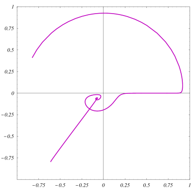
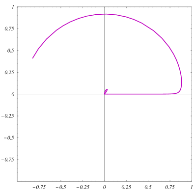
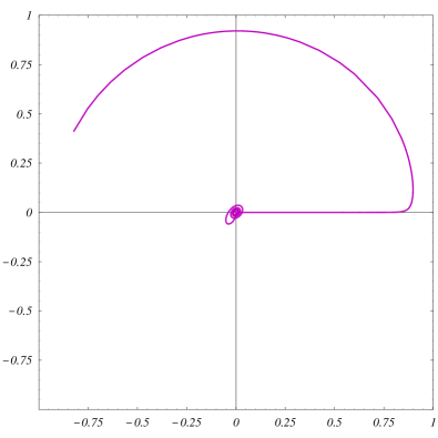
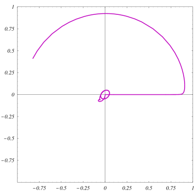
a)         b)
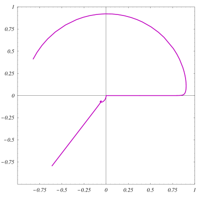
c)         d)
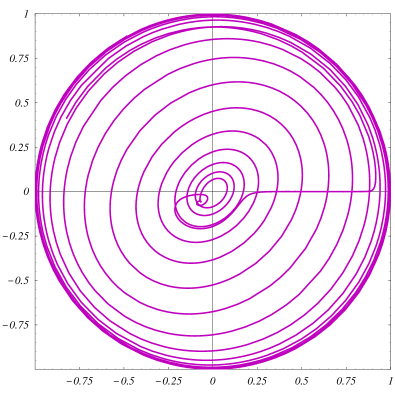
e)         f)

Figure 1: The evolution of quintessence projected to the $\{x,y\}$ plane at slope $\lambda=20$ with various parameters of potential $z_{\star}$ and matter state equations $w_{B}$ as described in the text.

At $|z_{\star}|>3$ critical points (52) take complex values, while matrices satisfy $\hat{B}_{a}=\hat{B}_{b}^{*}$, i.e. they are complex conjugate to each other as well as $x_{\star}=y_{\star}^{*}$. The same is valid for eigenvectors:

$$\boldsymbol{e}^{a}_{1}=\left(\begin{array}[]{c}3-\sqrt{9-z_{\star}^{2}}\\ z_{\star}\\ \end{array}\right),\quad\boldsymbol{e}^{a}_{2}=\left(\begin{array}[]{c}3+\sqrt{9-z_{\star}^{2}}\\ -z_{\star}\\ \end{array}\right),$$ (55)

while $\boldsymbol{e}^{b}_{1,2}=\{\boldsymbol{e}^{a}_{1,2}\}^{*}$. Basis (55) is orthonormal:

$$\boldsymbol{e}^{a}_{i}\cdot\boldsymbol{e}^{a}_{j}=\delta_{ij}.$$

The linearized system has solutions

$$\left(\begin{array}[]{c}x\\ y\\ \end{array}\right)=\left(\begin{array}[]{c}x_{\star}\\ y_{\star}\\ \end{array}\right)+\sum\limits_{j=1}^{2}\boldsymbol{e}^{a}_{j}\,u_{j}\,{\rm e}^{\nu^{a}_{j}N},$$ (56)

where $u_{j}$ stand for some initial data. Solutions (56) are complex-valued. By our investigation, (56) are irrelevant to physical quantities in question at $|z_{\star}|>3$.

III. Tuned scaling appears at the special value of parameter $z_{\scriptscriptstyle T}=3\sqrt{1-w_{B}^{2}}$. Then, there is the critical line

$$\mbox{(iii): ~{} }y_{\star}=x_{\star}\sqrt{\frac{1-w_{B}}{1+w_{B}}},$$ (57)

which is $\lambda$-invariant, i.e. independent of slope in the potential. It is spectacular that tuned point given by $z_{\scriptscriptstyle T}=z_{c}$, $x_{\star}=x_{c}$, $y_{\star}=y_{c}$ corresponds to the exact scaling solution found in Section II.

At (57) the linear analysis of perturbations gives two eigenvalues: $\nu_{1}=0$ and $\nu_{2}=2w_{B}$, so that zero eigenvalue corresponds to the line itself, while the positive one indicates instability at $w_{B}>0$ in vicinity of the line as a whole. This fact is in agreement with the study of critical points in the case II, since (57) contains the point of (52) at $w_{B}<0$ as well as it does the point at $w_{B}>0$ after the action of symmetry $\mathcal{B}$, so we correspondingly get eigenvalues (53) and (54) at $z_{\star}=z_{\scriptscriptstyle T}$ yielding the same result above. Therefore, at $w_{B}>0$ the scaling solution of section II is unstable in future, while it does at $w_{B}<0$.

IV. The boundary circle

$$\mbox{(iv): ~{} }x^{2}+y^{2}=1$$ (58)

is conserved by the autonomous system. This fact implies that at $|z_{\star}|>3$ and $w_{B}>0$, when there are no stable critical points, the system approaches the boundary circle in future.

Summarizing the results, we have found that in the presence of cosmological constant the scalar field with the hyper-cosine potential approaches the stable attractor at late times just before the present day (the time of cosmological constant becomes visible) at the potential slope $\lambda^{2}>3(1+w_{B})$, so that the energy of field scales like that of matter with the state parameter $w_{B}$, while the fraction of field energy depends on the slope value. However, this attractor exhibits the strange behavior in future, i.e. under the dominance of cosmological term. Then, the balance of remnant energy depends on the parameter $z_{\star}$ determined by two quantities: i) the weight of potential normalization with respect to the energy density due to the cosmological constant and ii) the slope, in accordance with (47). So, at $|z_{\star}|<3$ and $w_{B}\geqslant 0$ the dynamical part of scalar field energy reaches the other scaling attractor, which dominates over the matter in accordance with (53) (see Fig. 1a) and gets the state parameter

$$\widetilde{w}_{\phi}=-\sqrt{1-\frac{z_{\star}^{2}}{9}}.$$ (59)

At $|z_{\star}|<3$ and $w_{B}<0$ we get an interplay of two attractors with (51) and (53): at $3w_{B}+\sqrt{9-z_{\star}^{2}}<0$ the scalar field relaxes at the minimum of kinetic and potential energy (48) (see Fig. 1b), while, otherwise, at $3w_{B}+\sqrt{9-z_{\star}^{2}}>0$ the scalar field dominates over the matter at the same point of (53) and (59) (see Fig. 1c).

At $|z_{\star}|>3$ we get three cases: i) at $w_{B}>0$ the quintessence in future vibrates at the boundary circle as the limit cycle (see Fig. 1e), ii) at $w_{B}=0$ the field cycled around the center being the point of minimal kinetic and potential energy (see Fig. 1f), iii) at $w_{B}<0$ the field relaxes to the minimum (see Fig. 1d).

The evolution kinds of scalar field in the plane of $\{x,y\}$ are illustrated in Fig. 1 at $\lambda=20$ and various sets of $z_{\star}$ and $w_{B}$: at $z_{\star}=2.9$ we put $w_{B}=0.2$ in Fig. 1 a), $w_{B}=-0.5$ in b), and $w_{B}=-0.2$ in c), while at $z_{\star}=10$ we put $w_{B}=-0.2$ in Fig. 1 d), $w_{B}=0.2$ in e), and $w_{B}=0$ in f). At all of tries the evolution starts at $x_{0}=-0.8$, $y_{0}=0.4$, and trajectories move clockwise. We certainly see that trajectories approaches the late time attractor at appropriate $\{x_{c},y_{c}\}$, which are negative in all cases except b), when they are positive. The future attractors in Fig. 1 a) and c) are posed at $\{x_{\star},y_{\star}\}$ with opposite, negative, sign of (52). The attractors at b) and d) stand in the minimum, while limit cycles of e) and f) are at the border and around the minimum, correspondingly.

Thus, in the linear analysis we have classified the late time and future attractors for the quintessence with the specified kind of potential relevant to the case of nonzero cosmological constant.

However, this analysis falls in special degenerate case of $z_{\star}=3$, $w_{B}=0$.

III.3 Degenerate case

At $z_{\star}=3$, $w_{B}=0$ and $v\gg 1$ the analysis of future evolution becomes nonlinear, since, after the transformation to variables $\sigma=x^{2}+y^{2}$ and $\tau=x/y$, autonomous system (43) is reduced to

$$\begin{array}[]{l}\displaystyle\sigma^{\prime}=3\sigma(\sigma-1)\,\frac{1-\tau^{2}}{1+\tau^{2}},\\[8.53581pt] \displaystyle\tau^{\prime}=-\frac{3}{2}(1-\tau)^{2},\\ \end{array}$$ (60)

which can be solved explicitly. Indeed, the integration for $\tau$ results in

$$\tau=1+\frac{2}{\mathfrak{N}},$$ (61)

where $\mathfrak{N}=3(N-N_{0})$, and $N_{0}$ corresponds to some initial data. Hence, $\tau\to 1$ at the end of evolution, i.e. at $N\to+\infty$. Then,

$$\begin{array}[]{rcl}\displaystyle{\rm i}\ln\frac{1-\sigma}{1-\sigma_{0}}\,\frac{\sigma_{0}}{\sigma}&=&\displaystyle\ln\frac{\mathfrak{N}-\mathfrak{N}_{c}}{\mathfrak{N}-\mathfrak{N}_{c}^{*}}+\mathfrak{N}_{c}\ln(\mathfrak{N}-\mathfrak{N}_{c})\\[11.38109pt] &&\displaystyle-\mathfrak{N}_{c}^{*}\ln(\mathfrak{N}-\mathfrak{N}_{c}^{*}),\\[2.84526pt] \end{array}$$ (62)

where $\sigma_{0}<1$, $\mathfrak{N}_{c}=-(1+{\rm i})$. Therefore, at $N\to+\infty$ we find

$$\ln\frac{1-\sigma}{1-\sigma_{0}}\,\frac{\sigma_{0}}{\sigma}\to-2\ln N\to-\infty,$$

that implies

$$\sigma\to 1,$$ (63)

and the attractor is posed at the boundary circle,

$$x_{\star}=y_{\star}=\frac{1}{\sqrt{2}}\quad\mbox{or}\quad x_{\star}=y_{\star}=-\frac{1}{\sqrt{2}}.$$ (64)

If the initial data $\sigma_{0}=1$, the quantity $\sigma$ does not evolve, while $\tau$ approaches the attractor $\tau_{\star}=1$.

In addition, we have explicitly found that the second critical point $\sigma_{\star}=0$, i.e. $x_{\star}=y_{\star}=0$ is unstable.

The character of attractor (64) is illustrated in Fig. 2, where trajectories move clockwise.

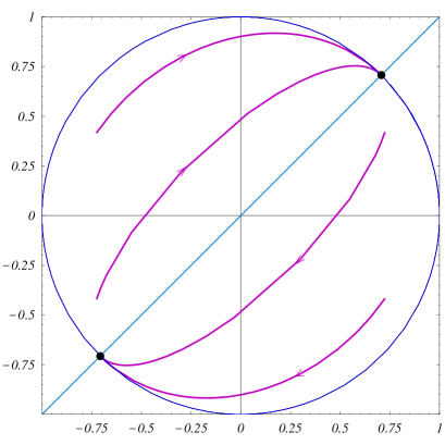
Figure 2: The attraction of trajectories to the critical points at the boundary circle of $\{x,y\}$ plane in the degenerate case.

Thus, attractors (64) exhibit the stable behavior in appropriate semicircles, while the line connecting the critical points has the instability versus perturbations.

IV Phenomenological points

IV.1 The mass

The potential of quintessence suggests the mass

$$m^{2}=\frac{\partial^{2}V}{\partial\phi^{2}}\Big{|}_{\phi=0}=4\pi G\lambda^{2}\widetilde{V}_{0}.$$ (65)

For the exact scaling solution in Section II we get

$$m^{2}_{s}=\frac{9}{4}\,(1-w_{B}^{2})\,H_{0}^{2}\Omega_{\Lambda},$$ (66)

and at $w_{B}=0$ and $\Omega_{\Lambda}\approx 0.7$ of practice the mass is determined by the current value of Hubble constant, i.e. it is extremely small as well as the energy scale of cosmological constant, that is beyond a natural reason. Although, such the mass could argue for both the present acceleration in the universe expansion and the scale of cosmological constant.

Generically, we get

$$m^{2}=\frac{2\pi}{3}\,V_{0}G\,z_{\star}^{2}=\frac{1}{4}\,H_{0}^{2}\Omega_{\Lambda}\,z_{\star}^{2}.$$ (67)

So, the mass of scalar quintessence scales as the present day Hubble constant with the factor of $z_{\star}$, which could be arbitrary to enlarge the mass up to reasonable values in the physics of Standard model. However, huge values of $z_{\star}$ involve extremely frequent oscillations of quintessence in the nearest future, that is in contradiction with the present smooth evolution of universe. Therefore, we expect that a viable model includes the quintessence mass of the order of Hubble constant today.

IV.2 Restriction to the slope

The late time scaling of quintessence results in a fixed fraction of quintessence energy in the budget of universe with respect to other matter irrespective of the evolution stage: the dust or radiation fix close values of fractions. However, the fraction of nonbaryonic matter is constrained due to measured and primordial abundances of light elements caused by Big Bang Nucleosynthesis Wetterich ; CLW . Then, the slope of potential should be quite large to suppress $\Omega_{\phi}\leqslant 0.13$, so according CLW one gets

$$\lambda^{2}>20.$$ (68)

Next, a role of quintessence field $\phi$ during inflation actually was analyzed in CLW , since the hyper-sine in fact coincides with the exponential potential at large values of field. The problem is a relic abundance of quintessence after inflation, that should be small in order to conserve the standard scenario of nucleosynthesis. Appropriate restrictions in various schemes of inflation are given in CLW .

IV.3 Initial conditions

Attractors mean a slow dependence of late time evolution on initial data for the quintessence. The character of regulation is illustrated in Fig. 3. The set of tries exhibits the following general features:

• At small initial fraction of quintessence energy, it is frozen to a moment, when it approaches an appropriate scaling value in order to start the tracker behavior at late times.

• At large initial fraction of quintessence energy, it rapidly falls in order to frozen and wait for a moment of tracker way at late times.

• In future, vibrations of quintessence at $z_{\star}>3$ and $w_{B}\geqslant 0$ determine an average value of dynamical parameter for the equation of state $\langle\widetilde{w}_{\phi}\rangle$, which is independent of initial data, whereas $-1<\langle\widetilde{w}_{\phi}\rangle<w_{B}$ at $w_{B}>0$ or $\langle\widetilde{w}_{\phi}\rangle=0$ at $w_{B}=0$ (see Fig. 3 a, b, c, d). At $w_{B}<0$ vibrations determine the effective $\langle\widetilde{w}_{\phi}\rangle>w_{B}$ (see Fig. 3 g, h).

Further observations repeat general properties of future attractors.

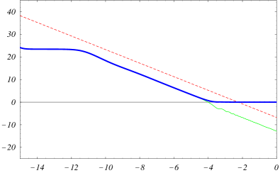
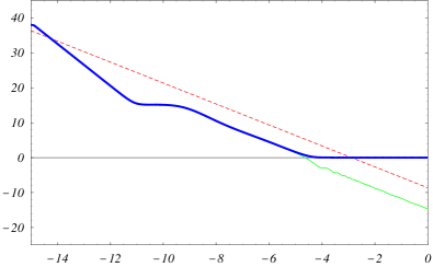
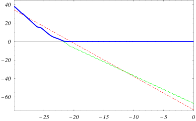
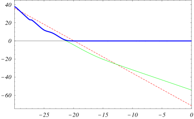
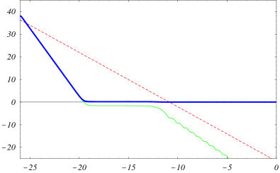
a)         b)
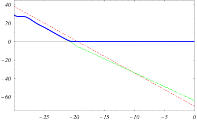
c)         d)
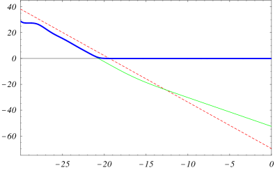
e)         f)
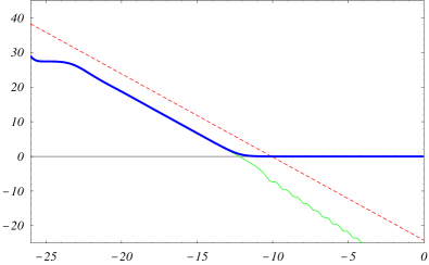
g)         h)

Figure 3: Approaching the scaling under different initial data: the logarithm of energy $\ln\rho$ in arbitrary units versus the e-folding $N=\ln a(t)$ with a casual shift of present day scale factor $a(t_{0})$; the quintessence and baryotropic matter are represented by thick solid and dashed lines, correspondingly, while the dynamical part of quintessence without the cosmological term is given by thin solid line. Initial data for the suppressed and dominated quintessence are respectively shown in left and right panels: a) and b) at $\lambda=20$, $w_{B}=0$ and $z_{\star}=50$; c) and d) at $\lambda=20$, $w_{B}=0.2$ and $z_{\star}=10$; e) and f) at $\lambda=20$, $w_{B}=0.2$ and $z_{\star}=2.9$; g) and h) at $\lambda=20$, $w_{B}=-0.2$ and $z_{\star}=10$.

IV.4 Equation of state

At late times, the attractor causes the ratio of quintessence pressure to the energy density $w_{\phi}$ is stabilized infinitely close to the value of parameter $w_{B}$ for the matter. However, the situation changes, when the cosmological term comes to dominate, and $w_{\phi}$ moves to $-1$. An example of $w_{\phi}$ relaxation is shown in Fig. 4 for the quintessence vibrating around the minimum point (see Figs. 1 f and 3 a, b). The present day e-folding is arbitrary in Fig. 4. The magnitude of deviation from the limit of $-1$ and vibration period depend on the potential parameters. The picture analogous to Fig. 4 was observed in BarreiroCN with similar values of parameters.

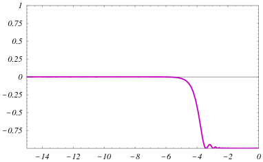
Figure 4: The state parameter of quintessence $w_{\phi}$ versus the e-folding $N$ of evolution scale: changing the stable value of late times at $w_{B}=0$ at $z_{\star}=50$ and $\lambda=20$.

It is clear that vibrations are absent if $z_{\star}<3$. Anyway, the parameter of quintessence state $w_{\phi}$ rapidly approaches the vacuum value. Nevertheless, it would be interesting to see a relative significance of quintessence with respect to the matter. So, general consideration of attractors and Fig. 3 demonstrate that the quintessence fraction can dominate or be suppressed depending on the potential parameters, the value of $z_{\star}$. It is evident that in the case of reaching the boundary circle in the $\{x,y\}$ plane the effective, average value for the state parameter is $\langle\widetilde{w}_{\phi}\rangle=0$, while the same value is clearly observed also in the case of $w_{B}=0$ and $|z_{\star}|>3$ (see Fig. 3 a and b).

Thus, we get the definite understanding of phenomenological properties for the evolution of quintessence with the specified kind of potential in the presence of cosmological term.

V Conclusion

In this paper we have found the potential of scalar field quintessence, which gives the exact solution for the scaling evolution of flat universe in the presence of cosmological constant. The scaling behavior is consistent with the current empirical observations.

We have investigated the stability of scaling behavior versus the variations in the slope and normalization of potential as well as in initial data. The analysis has revealed two kinds of attractors. The late time attractor just before the cosmological constant is coming to play, is independent of normalization, and it is determined by the slope, that is consistent with the well-known result for the exponential potentials CLW , representing the limit of large field for the potential found in the paper. The future behavior of quintessence under the dominance of cosmological constant depends on both the ratio of potential normalization to the vacuum energy density and slope in the special combination denoted by parameter $z_{\star}$. Generically, the future attractor differs from that of late time. So, the late time attractor reveals the strange behavior. We have classified the future attractors by their character and stability in linear analysis. The degenerate case of nonlinear dependence has been solved explicitly. Some phenomenological items have been considered, too.

We conclude that analysis of scaling attractors can be useful for classifying the quintessence behavior at late times and in future.

This work is partially supported by the Russian Foundation for Basic Research, grant 04-02-17530.

References

-
(1)
A. G. Riess et al. [Supernova Search Team
Collaboration],
Astron. J. 116, 1009 (1998) [arXiv:astro-ph/9805201];
B. P. Schmidt et al. [Supernova Search Team Collaboration], Astrophys. J. 507, 46 (1998) [arXiv:astro-ph/9805200];
S. Perlmutter et al. [Supernova Cosmology Project Collaboration], Astrophys. J. 517, 565 (1999) [arXiv:astro-ph/9812133];
J. P. Blakeslee et al. [Supernova Search Team Collaboration], Astrophys. J. 589, 693 (2003) [arXiv:astro-ph/0302402];
A. G. Riess et al. [Supernova Search Team Collaboration], Astrophys. J. 560, 49 (2001) [arXiv:astro-ph/0104455]. - (2) A. G. Riess et al. [Supernova Search Team Collaboration], Astrophys. J. 607, 665 (2004) [arXiv:astro-ph/0402512].
- (3) P. Astier et al., arXiv:astro-ph/0510447.
-
(4)
D. N. Spergel et al. [WMAP Collaboration],
Astrophys. J. Suppl. 148, 175 (2003)
[arXiv:astro-ph/0302209];
D. N. Spergel et al., arXiv:astro-ph/0603449. -
(5)
D. J. Eisenstein et al.,
arXiv:astro-ph/0501171;
S. Cole et al. [The 2dFGRS Collaboration], Mon. Not. Roy. Astron. Soc. 362, 505 (2005) [arXiv:astro-ph/0501174]. -
(6)
T. Chiba,
Phys. Rev. D 60, 083508 (1999)
[arXiv:gr-qc/9903094];
N. A. Bahcall, J. P. Ostriker, S. Perlmutter and P. J. Steinhardt, Science 284, 1481 (1999) [arXiv:astro-ph/9906463];
P. J. Steinhardt, L. M. Wang and I. Zlatev, Phys. Rev. D 59, 123504 (1999) [arXiv:astro-ph/9812313];
L. M. Wang, R. R. Caldwell, J. P. Ostriker and P. J. Steinhardt, Astrophys. J. 530, 17 (2000) [arXiv:astro-ph/9901388]. - (7) V. Sahni and A. Starobinsky, arXiv:astro-ph/0610026.
- (8) A. A. Starobinsky, JETP Lett. 68, 757 (1998) [Pisma Zh. Eksp. Teor. Fiz. 68, 721 (1998)] [arXiv:astro-ph/9810431].
- (9) M. Szydlowski, W. Godlowski and R. Wojtak, Gen. Rel. Grav. 38, 795 (2006) [arXiv:astro-ph/0505202].
- (10) C. Wetterich, Nucl. Phys. B 302, 668 (1988).
- (11) E. J. Copeland, A. R. Liddle and D. Wands, Phys. Rev. D 57, 4686 (1998) [arXiv:gr-qc/9711068].
- (12) P. G. Ferreira and M. Joyce, Phys. Rev. D 58, 023503 (1998) [arXiv:astro-ph/9711102].
- (13) A. Albrecht and C. Skordis, Phys. Rev. Lett. 84, 2076 (2000) [arXiv:astro-ph/9908085].
- (14) S. Tsujikawa, arXiv:hep-th/0601178.
- (15) Y. Gong, A. Wang and Y. Z. Zhang, Phys. Lett. B 636, 286 (2006) [arXiv:gr-qc/0603050].
- (16) V. Sahni and A. A. Starobinsky, Int. J. Mod. Phys. D 9, 373 (2000) [arXiv:astro-ph/9904398].
- (17) V. Sahni and L. M. Wang, Phys. Rev. D 62, 103517 (2000) [arXiv:astro-ph/9910097].
- (18) L. A. Urena-Lopez and T. Matos, Phys. Rev. D 62, 081302 (2000) [arXiv:astro-ph/0003364].
- (19) A. Gruppuso and F. Finelli, Phys. Rev. D 73, 023512 (2006) [arXiv:astro-ph/0512641].
- (20) A. A. Sen and S. Sethi, Phys. Lett. B 532, 159 (2002) [arXiv:gr-qc/0111082].
- (21) C. Rubano, P. Scudellaro, E. Piedipalumbo and S. Capozziello, Phys. Rev. D 68, 123501 (2003) [arXiv:astro-ph/0311535].
- (22) C. Rubano, P. Scudellaro, E. Piedipalumbo, S. Capozziello and M. Capone, Phys. Rev. D 69, 103510 (2004) [arXiv:astro-ph/0311537].
- (23) T. Barreiro, E. J. Copeland and N. J. Nunes, Phys. Rev. D 61, 127301 (2000) [arXiv:astro-ph/9910214].