Outer Trapped Surfaces In Vaidya Spacetimes

Abstract

It is proven that in Vaidya spacetimes of bounded total mass, the outer boundary, in spacetime, of the region containing outer trapped surfaces, is the event horizon. Further, it is shown that the region containing trapped surfaces in these spacetimes does not always extend to the event horizon.

1 Introduction

There has been renewed interest in the last several years in studying black holes from a more local perspective, including attempting to come up with a local definition for the boundaries of black holes. A black hole is defined as a region in spacetime that cannot be observed from infinity. The boundary of the black hole region is the event horizon. This is a 3-surface defined globally and therefore knowledge of the entire future evolution of the spacetime is required before the event horizon’s position and even existence are known. Turning next to local surfaces, the notion of an outer trapped surface was introduced in the studies of black holes. An outer trapped surface is a compact spacelike surface where the outgoing null geodesics orthogonal to the surface are initially converging, i.e. their expansion is negative. Examples of outer trapped surfaces are 2-spheres inside the event horizon in a Schwarzschild spacetime. Verifying that a surface is outer trapped only requires knowledge of the spacetime in a neighborhood of the surface. In this sense outer trapped surfaces are local while the event horizon, as mentioned, is global.

Assuming reasonable energy conditions and a non-nakedly singular spacetime, outer trapped surfaces lie entirely inside the event horizon [1]. In numerical applications locating these surfaces is of interest in finding the existence of a black hole surrounding them, since locating the event horizon is more difficult. Outer trapped surfaces are also useful in excision techniques, since outer trapped surfaces, and the region enclosed by them, lie entirely inside the black hole. Hence, modifying this region cannot affect the evolution outside the black hole and a numerical simulation can be carried out more easily.

Consider some time slice of the spacetime, i.e. a spacelike 3-surface in the spacetime. One could consider the region in this 3-surface containing outer trapped surfaces that lie entirely in this 3-surface. The outer boundary of this region is the apparent horizon. This is a spacelike 2-surface with the expansion of outgoing null geodesics orthogonal to it vanishing [1]. Given a foliation of the spacetime by spacelike 3-surfaces, the apparent horizon on each leaf of the foliation can be found, and one can consider the union of the apparent horizons on all such leafs. This is a 3-surface that will be referred to as the apparent 3-horizon, so as to distinguish it from the apparent horizon, a 2-surface on one time slice. In general, the apparent 3-horizon can be discontinuous. Furthermore, the apparent horizons in spacetime are not unique. A different foliation of the spacetime into spacelike surfaces can result in a different location of the apparent horizon through the spacetime. As a result the apparent 3-horizon is, in general, neither unique, nor continuous.

More recently, the notions of trapping horizons [2] and dynamical horizons [3] were introduced. These are 3-surfaces that, like the apparent horizon, are quasi-local and therefore do not require the entire evolution of the spacetime in order for them to be located. Though these surfaces are smooth by definition, they come with additional requirements. It is not known, in general, whether these surfaces always exist in spacetimes containing black holes. Furthermore, these 3-surfaces need not be unique.

As described, the apparent horizon is defined by restricting attention to outer trapped surfaces lying in a single time slice. Consider removing this restriction. Instead, consider the region in spacetime containing outer trapped surfaces. The outer boundary of this region is some unique 3-surface that is certainly independent of any slicing of the spacetime. This 3-surface has not been studied much in the past.

Even in spherically symmetric spacetimes, where, due to symmetry, finding apparent horizons on spherically symmetric slices is, relatively, an easy task, finding this 3-surface is not as easy. In spherically symmetric spacetimes, this 3-surface is spherically symmetric. However, the outer trapped surfaces contained within the region enclosed by this surface, need not be spherically symmetric. In fact, they need not lie in spherically symmetric slices. Not much is known about the locations of non-spherically symmetric outer trapped surfaces, and this is the main source of difficulty in locating this 3-surface.

Given some foliation of the spacetime, consider the apparent 3-horizon that is associated with this foliation. It is clear that the 3-surface, which is the boundary of the region containing outer trapped surfaces, lies outside of (or coincides with) the apparent 3-horizon and lies inside of (or coincides with) the event horizon. However, in general, the apparent 3-horizon and the event horizon can be separated in the dynamical regime, and therefore there is room for this 3-surface to lie somewhere in-between.

This point is well illustrated in Vaidya spacetimes, commonly used to describe gravitational collapse that ends in the formation of a black hole. The metric for a Vaidya spacetime is given by

$$g_{ab}=-\Big{(}1-\frac{R(v)}{r}\Big{)}dv_{a}dv_{b}+2dv_{(a}dr_{b)}+r^{2}\Big{(}d\theta_{a}d\theta_{b}+\sin^{2}\theta\,d\phi_{a}d\phi_{b}\Big{)}$$ (1)

with $R(v)$ some non-negative, non-decreasing, smooth function of $v$. In this work, $R(v)$ is also assumed to be bounded from above with a least upper bound, $R_{0}$. The stress energy is given by

$$T_{ab}=\frac{R^{\prime}(v)}{8\pi r^{2}}dv_{a}dv_{b}$$ (2)

The function $R(v)$ is non-negative to ensure a non-nakedly singular spacetime. It is non-decreasing in order for the spacetime to satisfy the dominant energy condition, as can be seen in (2). Finally, the additional requirement of it being bounded from above, is in order to guarantee that the spacetime is asymptotically flat and asymptotes to Schwarzschild.

This spherically symmetric spacetime describes the collapse of null dust in forming a black hole of mass $M=\frac{1}{2}R_{0}$. The metric is given in terms of the following coordinates. Advanced time, $v$, areal radius, $r$, and the usual angular coordinates, $\theta$ and $\phi$. In the special case $R(v)=2M$, with $M$ some positive constant, the metric is that of Schwarzschild in ingoing Eddington-Finkelstein coordinates.

Given any 2-sphere, i.e. a surface of constant $v$ and $r$, the expansion, $\Theta$, of outgoing null geodesics orthogonal to it is given by

$$\Theta\,=\,-\frac{2\big{(}R(v)-r\big{)}}{r^{2}}$$ (3)

Since the apparent horizon on any spherically symmetric slice of this spacetime is a 2-sphere, then it follows from (3) that the apparent horizon on any spherically symmetric asymptotically flat slice is the outermost 2-sphere satisfying $r=R(v)$ in that slice. Consider the spacelike 3-surface given by $r=R(v)$ for all $v$. Outside the $r=R(v)$ surface, 2-spheres are not outer trapped, while inside it, 2-spheres are outer trapped. The event horizon does not, in general, coincide with this 3-surface, and thus there exists, in general, a non-empty region between the surface $r=R(v)$ and the event horizon.

Moreover, notice that, in general, far in the past $R(v)$ may vanish and that region of the spacetime will be a portion of flat space. In fact, the spacetime where $R(v)=0$ for $v<v_{0}$ and $R(v)=2M$ for $v\geq v_{0}$, which can be obtained as a limit of a smooth family of such Vaidya spacetimes, describes the collapse of a thin null dust shell in flat space. A spacetime diagram of a thin null dust shell collapse is shown in Fig. 1.

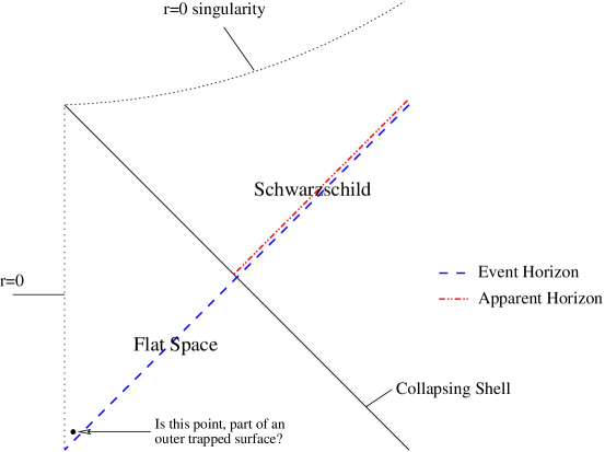
Figure 1: A spacetime diagram of the collapse of a thin null dust shell in flat space. Two angular dimensions are suppressed. Points in this diagram are, therefore, 2-spheres. The region to the left of the shell is a portion of flat space. The region to the right of it is a portion of a Schwarzschild spacetime. The event horizon, a null 3-surface, is shown. The point on the left represents a single event (as part of a 2-sphere). It lies inside the event horizon but is deep in the flat region. Is there an outer trapped surface that contains this point?

As can be seen in this figure, the event horizon extends into the flat region. But, it is known that there are no outer trapped surfaces in flat space. Indeed, the surface $r=R(v)$ does not extend into the flat region of the spacetime. What about the boundary of the region containing outer trapped surfaces? Could this 3-surface extend into the flat portion?

Eardley [5] conjectured that the boundary of the region that contains marginally outer trapped surfaces coincides with the event horizon. For this conjecture to be true, there need to exist marginally outer trapped surfaces close to the event horizon in the flat portion. For example, a marginally outer trapped surface must pass through the point shown in Fig. 1. However, as was just pointed, there are no marginally outer trapped surfaces in flat space. Could there be marginally outer trapped surfaces in this spacetime that lie, in part, in the flat portion?

In [5], Eardley gave an argument showing how one can get outer trapped surfaces, parts of which extend beyond the apparent horizon on some given slice. He then discussed how one might, in spacetimes such as the null shell collapse, find outer trapped surfaces that reach into the flat portion. The idea is to have a 2-surface that lies mostly far in the future, with a thin tendril that is almost null and lies near the event horizon. The tendril reaches into the flat portion and this 2-surface with a tendril is outer trapped.

The existence of non-spherically symmetric marginally trapped surfaces in Vaidya spacetimes was investigated numerically by Schnetter and Krishnan [6]. For specific choices of $R(v)$ they located marginally trapped surfaces, i.e. surfaces where both expansions are non-positive, that penetrate into part of the flat region of the Vaidya spacetime.

These results do not address Eardley’s conjecture. Eardley’s conjecture is about the boundary of the region containing (marginally) outer trapped surfaces, i.e. surfaces with no restriction on the expansion of ingoing null geodesics orthogonal to the 2-surface. In contrast, the surfaces found by Schnetter and Krishnan are marginally trapped, i.e. they satisfy the additional requirement that the ingoing expansion is everywhere non-positive. However, since trapped surfaces are, of course, also outer trapped, then Schnetter and Krishnan’s results show numerically that it is possible to find marginally outer trapped surfaces extending into the flat region of a Vaidya spacetime. Moreover, one can also consider the region containing trapped surfaces and its outer boundary. This boundary is some unique 3-surface that lies inside of (or coincides with) the event horizon. The numerical results of Schnetter and Krishnan show that this 3-surface can extend into the flat region of a Vaidya spacetime.

The main purpose of this work is to prove that in Vaidya spacetimes there are outer trapped surfaces extending arbitrarily close to the event horizon in any region of the spacetime. The event horizon, then, is the boundary of the region containing outer trapped surfaces and in this case Eardley’s conjecture is indeed true.

This will be achieved by constructing an outer trapped surface. Starting with the initial point that lies inside the event horizon, and which might be located in a flat portion, a spacelike narrow tube is constructed. This tube stays inside the event horizon and corresponds to Eardley’s tendril. The tube reaches inside the apparent horizon in the far future and it then tends to a region very close to the singularity. The idea is to close the surface off in a specific way once it is close to the singularity, thereby ensuring that the resulting surface is outer trapped. A sketch of this idea is shown in Fig. 2. Closing this tube into a surface shaped like a worm’s skin, could lead to an inner trapped surface as can be seen on the left. Inner trapped surfaces certainly exist in flat space. If instead the surface is closed off inside-out, like the face of Pacman, then it may be possible to obtain an outer trapped surface in this way, since this procedure interchanges the ingoing and outgoing directions, as can be seen on the right. Recall that inside the spherically symmetric apparent horizon, 2-spheres are outer trapped. Since the closing off is done in the far future, inside the apparent horizon, then it will be possible to keep the expansion negative in that region as well.

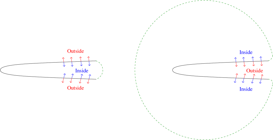
Figure 2: Left, a narrow tube shaped like a worm’s skin. The ingoing and outgoing directions are shown. Right, a similar tube closed off differently. Now it is closed inside-out, like the face of Pacman. As a result the ingoing and outgoing directions of the tube on the left, are interchanged. Therefore, a portion of an inner trapped surface (the worm) can be used in constructing an outer trapped surface (the Pacman). The specific closing off inside-out will be done in the far future, inside the apparent horizon, where 2-spheres are outer trapped.

It will also be shown in this work that in Vaidya spacetimes, the region containing trapped surfaces does not, in general, extend everywhere to the event horizon. As shown by Schnetter and Krishnan, the boundary of the region containing trapped surfaces may extend to the flat region of a Vaidya spacetime. However, the result obtained here shows that in general, this boundary is separated from the event horizon in the flat region.

2 Main result and key ideas

Consider a Vaidya spacetime with a metric given by (1) with $R(v)$ some non-negative, non-decreasing, smooth function of $v$ that is bounded from above with a least upper bound, $R_{0}$.

Since $R(v)$ is bounded by $R_{0}$ then this spacetime is asymptotically flat and tends to Schwarzschild spacetime in the far future. It follows that this spacetime (for the non-trivial $R_{0}\neq 0$ case) contains a spherically symmetric event horizon, which can be described by the equation $r=r_{eh}(v)$. The function $r_{eh}$ cannot be specified without full knowledge of the function $R(v)$. However, like $R(v)$, this function is non-decreasing and in addition $r_{eh}(v)\geq R(v)$ with equality holding at $v_{0}$ only if $R(v)$ is constant for all $v\geq v_{0}$ (i.e. if the spacetime is exactly Schwarzschild in the future). If the spacetime contains a flat region, i.e. if there exists some $v_{\text{flat}}$ such that $R(v)=0$ for all $v\leq v_{\text{flat}}$, then the event horizon extends to this region as well.

Consider a point in this spacetime that lies inside the event horizon, but may be arbitrarily close to it. It lies, in the coordinates above, at $r_{0}$ and $v_{0}$ satisfying $r_{0}<r_{eh}(v_{0})$ and, without loss of generality, this point is assumed to lie at $\theta=0$.

The main result of this work is a proof by construction of the existence of an outer trapped surface that contains this point. More precisely, the following proposition is proven:

Proposition: Given a Vaidya spacetime with metric as in (1) such that $R(v)$ is a non-negative, non-decreasing, bounded function with $R_{0}>0$ the least upper bound of $R(v)$, and given any point that lies inside the event horizon, then there exists a compact smooth spacelike 2-manifold, such that the expansion, $\Theta$, of outgoing future-directed null geodesics normal to it is everywhere negative.

This leads directly to the following result:

Corollary: In any Vaidya spacetime of bounded total mass, the outer boundary of the region containing outer trapped surfaces is the event horizon.

The proposition will be proved in the next section by direct construction. Before doing so, it is worthwhile to understand the general situation and the central ideas of the construction.

As discussed earlier, 2-spheres with $r<R(v)$ are outer trapped. Therefore, the challenge is to construct an outer trapped surface containing a point that is located at some given $r=r_{0}$ and $v=v_{0}$ such that $R(v_{0})<r_{0}<r_{eh}(v_{0})$.

Since the desired outer trapped surface cannot be spherically symmetric, the next simplest option is an axisymmetric surface. The first central idea in the present work is the particular way in which this surface is constructed. A spacelike vector field, $w^{a}$, is defined. This vector field is orthogonal to the axial Killing field, $c^{a}\equiv(\frac{\partial}{\partial\phi})^{a}$. The integral curve of $w^{a}$ that contains the initial point is chosen. This curve is then translated by the axial Killing field, $c^{a}$, and this results in a surface. Since the Killing field has closed orbits then provided that the integral curve starts and ends at the axis and does not intersect it in-between, the resulting surface will be compact. If $w^{a}$ is smooth then the surface obtained in this way is smooth except possibly for the north and south poles. Extra care will be taken at the poles to ensure the surface is smooth everywhere.

Next, consider the expansion, $\Theta$. The outgoing, future directed, null rays orthogonal to this surface are given by some null vector field $l^{a}$ such that $l^{a}$ is orthogonal to the vector fields $w^{a}$ and $c^{a}$. There still remains a scaling freedom for $l^{a}$. However, this freedom does not affect the sign of the expansion, and since for a surface to be outer trapped it is the sign of the expansion that matters, then any convenient choice will do.

The expansion of $l^{a}$ is given by $\Theta=q^{ab}\nabla_{a}l_{b}$ where $\nabla_{a}$ is the covariant derivative associated with $g_{ab}$ and $q^{ab}$ is the inverse of the induced metric on the 2-surface given by

$$q^{ab}=\frac{w^{a}w^{b}}{w^{c}w_{c}}+\frac{c^{a}c^{b}}{c^{c}c_{c}}$$ (4)

Given a choice of a spacelike vector field $w^{a}$ as above, such that the expansion of outgoing null rays, $l^{a}$, is negative along the integral curve of $w^{a}$ then the surface obtained in this way is, as desired, an outer trapped surface.

There are other, more direct, ways of specifying a 2-surface in spacetime. For example, two functions in spacetime could be defined such that the intersection of two level surfaces of these functions is a 2-surface. However, it is much more difficult to use such direct methods for all Vaidya spacetimes with a metric as in (1) and with any $R(v)$ that satisfies the conditions above, since they require the global specification of the surface “all at once” such that $\Theta<0$ everywhere. Instead, using the method employed here, one defines a vector field in spacetime. This allows one to make appropriate “local adjustments” to the surface in the process of defining it. Thus, one is able to ensure that the expansion is negative by such “local adjustments”.

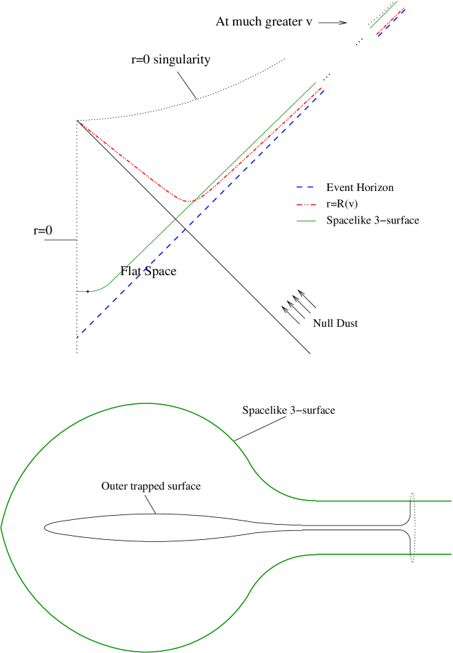
Figure 3: Top: A spacetime diagram of a Vaidya spacetime. Two angular dimensions are suppressed. Points in this diagram are, therefore, 2-spheres. A spherically symmetric spacelike 3-surface is shown. Bottom: A schematic of this 3-surface. One angular dimension is not shown. The desired outer trapped surface is the line traced on this 3-surface.

The central idea leading to a suitable choice of the vector field, $w^{a}$, is that proximity to the axis combined with a specific closing of the 2-surface will enable maintaining the expansion negative. This was described earlier and was shown in Fig. 2. Fig. 3 shows how this idea is actually implemented in a Vaidya spacetime. The top diagram is a spacetime diagram of the collapse of null dust in flat space. In this diagram a spherically symmetric spacelike slice that contains the desired outer trapped surface is shown. The bottom diagram depicts this spacelike 3-surface. The outer trapped surface including its angular ($\theta$) dependence is shown as a line in this 3-surface. As can be seen in the bottom diagram of Fig. 3, the outer trapped surface remains close to the axis for the most part, i.e. at a very small $\theta$. Once the conditions are right, the 2-surface closes off in the particular way described earlier, as can be seen at the right side of the bottom diagram.

A sketch of the construction is now given. Full details are given in the next section. In what follows the components of the vector fields are given with respect to the coordinates $v,r$, and $\theta$ used in the metric above.

The vector field $w^{a}$ is constructed by a sequence of smooth transitions between five vector fields. Each one of these is used only in a restricted region of the spacetime. This is achieved by taking $w^{a}$ to be of the form:

$$w^{a} = (1-\alpha_{1,2})w_{1}^{\ a}+\alpha_{1,2}(1-\alpha_{2,3})w_{2}^{\ a}+\alpha_{2,3}(1-\alpha_{3,4})w_{3}^{\ a}$$ (5)

$$+ \alpha_{3,4}\,\cos\alpha_{4,5}\,w_{4}^{\ a}+\sin\alpha_{4,5}\,w_{5}^{\ a}$$

and the five vector fields are given by

$$w_{1}^{\ a} =\ 2R_{0}\,r\sin\theta\Big{(}\frac{\partial}{\partial v}\Big{)}^{a}+2R_{0}\Big{(}r-\frac{R(v)}{2}\Big{)}\sin\theta\Big{(}\frac{\partial}{\partial r}\Big{)}^{a}$$

$$+\Big{(}2R_{0}\cos\theta\ -r\Big{)}\Big{(}\frac{\partial}{\partial\theta}\Big{)}^{a}$$ (6)

$$w_{2}^{\ a} =2\Big{(}\frac{\partial}{\partial v}\Big{)}^{a}$$

$$+\Big{(}1-\frac{R(v)}{r}+\frac{\sqrt{4R_{0}^{\ 2}-4R_{0}\,r\cos\theta+r^{2}}-(2R_{0}\cos\theta\,-r)}{\sqrt{4R_{0}^{\ 2}-4R_{0}\,r\cos\theta+r^{2}}+(2R_{0}\cos\theta\,-r)}\Big{)}\Big{(}\frac{\partial}{\partial r}\Big{)}^{a}$$ (7)

$$w_{3}^{\ a} =2\Big{(}\frac{\partial}{\partial v}\Big{)}^{a}+\Big{(}1-\frac{R(v)}{r}(1-\frac{\epsilon}{r})\Big{)}\Big{(}\frac{\partial}{\partial r}\Big{)}^{a}\$$ (8)

$$w_{4}^{\ a} =2\Big{(}\frac{\partial}{\partial v}\Big{)}^{a}$$ (9)

$$w_{5}^{\ a} =\frac{2}{r}\,\sqrt{1-\frac{R(v)}{r}}\,\Big{(}\frac{\partial}{\partial\theta}\Big{)}^{a}$$ (10)

where $\epsilon$ is some positive constant to be specified later.

The functions $\alpha_{i,i+1}$ appearing in (5), are referred to as transition functions, i.e. these are functions that facilitate the transition from one vector field to the next. Except for the last transition function, $\alpha_{4,5}$, the functions $\alpha_{i,i+1}$ are all smooth, non-decreasing functions of $v$ into $[0,1]$, and are chosen so that in a neighborhood where one such $\alpha$ is not identically $0$ or $1$ then all the other $\alpha$s are fixed to either $0$ or $1$ identically there. This can be explained more clearly as follows: The smooth functions $\alpha_{i,i+1}$ result in the division of the spacetime into several disjoint regions that border each other. First, there is a region where $w^{a}=w_{1}^{\ a}$. This region contains the initial point. Next, there is a transition region where $w^{a}$ is a smooth linear combination of $w_{1}^{\ a}$ and $w_{2}^{\ a}$. The next region is such that $w^{a}=w_{2}^{\ a}$ there. This is followed by another transition region, and so on. The integral curve that starts at the initial point will be shown to traverse all these different regions.

Here is a rough description of what this surface is like. Initially the surface starts at $\theta=0$ and $\theta$ increases to some small fixed value. Meanwhile, the surface continues towards increasing $v$ and $r$, tending closer to the event horizon. In the top diagram of Fig. 3, this is the horizontal part of the 3-surface in a small neighborhood of the initial point. Next, the surface starts following the event horizon into the future at constant $\theta$, always remaining inside the event horizon. At late $v$ – when the 3-surface $r=R(v)$ tends to the event horizon as the spacetime asymptotes to Schwarzschild – the constructed surface is finally inside the 3-surface $r=R(v)$, as can be seen in the top diagram of Fig. 3. At this stage $r$ starts decreasing. This is shown in the bottom diagram of Fig. 3. The surface, next, settles to very small $r$, close to the black hole singularity. This can be seen in the top diagram of Fig. 3, at much larger $v$. In the bottom diagram, this is the part where the geometry tends to a cylinder with a constant thickness. Finally, the surface closes off like a 2-sphere, following the idea described earlier, as shown in the bottom diagram of Fig. 3.

3 Details

The proposition is now proved by presenting the full details of the construction.

Given a metric of the form (1) with $R(v)$ satisfying the conditions above, consider an event, i.e. a point in this spacetime, which without loss of generality can be taken to lie at the north pole, $\theta=0$, at some $v=v_{0}$ and $r=r_{0}$ such that $R(v_{0})<r_{0}<r_{eh}(v_{0})$. The first inequality here ensures that finding an outer trapped surface is non-trivial, since if $r_{0}$ were smaller than $R(v_{0})$ then the 2-sphere with constant $r$ and $v$ passing through the point would be outer trapped. The second inequality follows since the point of interest lies strictly inside the event horizon (though perhaps arbitrarily close to it).

The following notation is used. Let $v_{i},r_{i}$, and $\theta_{i}$ stand for the value of the coordinates $v,r$, and $\theta$ respectively, when the transition from $w_{i}^{\ a}$ to $w_{i+1}^{\ \ \ a}$ starts. Let $v_{i,i+1},r_{i,i+1}$, and $\theta_{i,i+1}$ be the values of these coordinates at the end of the transition to $w_{i+1}^{\ \ \ a}$.

Given the value of $w^{a}$ in some region, one needs an expression for $l^{a}$ in order to evaluate the expansion. Since $l^{a}$ can be rescaled by an arbitrary function, there remains some freedom in choosing the components of $l^{a}$. Here, a choice will be made by fixing the component of $l^{a}$ along $(\frac{\partial}{\partial v})^{a}$ to be two. The components of $l^{a}$ along $(\frac{\partial}{\partial r})^{a}$ and $(\frac{\partial}{\partial\theta})^{a}$ can then be uniquely determined as follows. The two conditions $l^{a}l_{a}=0$ and $l^{a}w_{a}=0$ translate into equations that when solved uniquely determine the component along $(\frac{\partial}{\partial r})^{a}$. These also yield two possible solutions for $(\frac{\partial}{\partial\theta})^{a}$ since the conditions used so far allow $l^{a}$ to be either outgoing or ingoing. The outgoing direction, as discussed earlier and shown in Fig. 3 is the solution tending towards smaller $\theta$, i.e. the more negative solution. This procedure is followed for the entire sequence of transitions including during the transitions themselves.

Using (4), the expansion, $\Theta$, can be written as:

$$\Theta(w) = q^{ab}\nabla_{a}l_{b}$$ (11)

$$= \Big{(}\frac{w^{a}w^{b}}{w^{c}w_{c}}+\frac{c^{a}c^{b}}{c^{c}c_{c}}\Big{)}\nabla_{a}l_{b}$$

$$= -\frac{w^{a}l^{b}\nabla_{a}w_{b}}{w^{c}w_{c}}+\frac{c^{a}l^{b}\nabla_{b}c_{a}}{c^{c}c_{c}}$$

$$= -\frac{w^{a}l^{b}\nabla_{a}w_{b}}{w^{c}w_{c}}+\frac{1}{2}l^{b}\nabla_{b}\log(c^{a}c_{a})$$

where in the third equality, $l^{a}w_{a}=0$ was used in getting the first term and $l^{a}c_{a}=0$ and $c^{a}$ being a Killing vector field were used in getting the second term. Throughout this work the expansion is evaluated using this expression.

Getting an outer trapped surface requires precise control over the location of the integral curve. This is achieved with a suitable tuning of the transition functions $\alpha_{i,i+1}$ that control the five vector fields and basically turn the vector fields on and off in certain regions of the spacetime.

Except for the final transition, from $w_{4}^{\ a}$ to $w_{5}^{\ a}$, all the transitions are taken to be of the form

$$w^{a}=\Big{(}1-\alpha_{i,i+1}(v)\Big{)}w_{i}^{\ a}+\alpha_{i,i+1}(v)w_{i+1}^{\ \ \ a}$$ (12)

As functions of $v$ this means that $w^{a}$, except for the final transition, simply changes with $v$ as follows. At $v\leq v_{1}$, $w^{a}=w_{1}^{\ a}$. A transition via $\alpha_{1,2}$ takes place and at any intermediate $v$, i.e. $v_{1}<v<v_{1,2}$, the vector field $w^{a}$ is some linear combination of $w_{1}^{\ a}$ and $w_{2}^{\ a}$. At $v_{1,2}\leq v\leq v_{2}$, $w^{a}=w_{2}^{\ a}$, and so on.

For simplicity, the form of the transition is picked once and is used repeatedly. Pick a smooth function $f(x)$ such that $f(x)$ is non-decreasing, $f(x)=0$ for $x\leq 0$, $f(x)=1$ for $x\geq 1$, and finally $f^{\prime}(x)>0\ \forall x\in(0,1)$. Given this choice of $f(x)$, all of the transition functions, except the last one, will be of the form

$$\alpha_{i,i+1}(v)=f\Big{(}\lambda(v-v_{i})\Big{)}$$ (13)

with $\lambda=\frac{1}{v_{i,i+1}-v_{i}}$. It follows that $\alpha_{i,i+1}(v)=0$ for $v\leq v_{i}$ and that $\alpha_{i,i+1}(v)=1$ for $v\geq v_{i,i+1}$.

As a result of using this canonical transition, it remains only to choose the various starting and ending regions for the transitions. In each transition it will be shown that with the choices made, the integral curve along $w^{a}$ reaches the desired regions and the expansion along the integral curve of $w^{a}$ is always negative.

Two parameters will be used in the choosing of the beginning and ending regions for the transition functions. These are given by

$$\epsilon = \min\Big{(}\frac{r_{eh}(v_{0})-r_{0}}{7},\,\epsilon^{*},\,\frac{R_{0}}{16}\Big{)}$$ (14)

$$\tilde{\theta} = \min\Big{(}\frac{\sqrt{\epsilon\,R_{+}}}{2R_{0}},\,\sqrt{\frac{\epsilon}{v^{*}_{r_{0}}-v_{0}}},\,\theta^{*}_{1},\,\theta^{*}_{2},\,\theta^{*}_{3},\,\frac{\pi}{8}\Big{)}$$ (15)

where $v^{*}_{r_{0}}$ satisfies $R(v^{*}_{r_{0}})=r_{0}$, and $R_{+}$ is given by

$$R_{+} = \left\{\begin{array}[]{l@{\quad\quad\quad}l}\frac{1}{2}R(v_{0}),&R(v_{0})>0\vspace{5pt}\\ \frac{1}{2}r_{0},&R(v_{0})=0\\ \end{array}\right.$$ (18)

The parameters $\theta^{*}_{1},\theta^{*}_{2},\theta^{*}_{3}\text{, and }\epsilon^{*}$ are chosen in the following sections. The choice of $\theta^{*}_{1}$ is made at the end of Section 3.1. $\theta^{*}_{2}$ is chosen in Section 3.2. The choice of $\theta^{*}_{3}$ is made at the beginning of Section 3.3. Finally, $\epsilon^{*}$ is chosen in Section 3.5. It is important to note that the choices of $\theta^{*}_{1},\,\theta^{*}_{2},\,\theta^{*}_{3},\text{and }\epsilon^{*}$ are all independent of each other. The specification of $\theta^{*}_{1},\,\theta^{*}_{2},\,\theta^{*}_{3},\text{and }\epsilon^{*}$ is discussed later purely for convenience, so that the relevant conditions for making these specifications will be at hand.

Since $\theta^{*}_{1},\,\theta^{*}_{2},\,\theta^{*}_{3},\text{and }\epsilon^{*}$ are all positive then it follows that $\tilde{\theta}$ and $\epsilon$ are positive as well. The reasons for these choices will be clear once the parameters are used in the construction.

Along the integral curve $r$ can be considered as a function of $v$ and therefore it is possible to define the following function:

$$\tilde{r}(v)\equiv r(v)-r_{eh}(v)$$ (19)

This function serves to keep track of where is the integral curve relative to the event horizon, for a given $v$.

3.1 Initially $w^{a}=w_{1}^{\ a}$ : Starting at the north pole

At the initial point, at the north pole, the construction starts with $w^{a}=w_{1}^{\ a}$ where $w_{1}^{\ a}$ was given  by (6).

As mentioned earlier, the north pole, $\theta=0$, is one point where extra care must be taken to ensure the surface is smooth. This choice of $w_{1}^{\ a}$ guarantees that the resulting surface will be smooth at the north pole as follows. The integral curve of $w_{1}^{\ a}$ near the north pole can be parametrized by $\mu=\cos\theta$. This gives a system of ordinary differential equations for $v$ and $r$ as functions of $\mu$ with smooth coefficients in a neighborhood of the north pole. It follows that in a neighborhood of the north pole, in the resulting surface, $v$ and $r$ are smooth functions of $\mu$. Changing into Cartesian coordinates one can then verify that the surface is smooth at the north pole.

The outgoing null vector field, $l^{a}$, is needed for evaluating the expansion. Following the procedure discussed earlier, it is found to be

$$l_{1}^{\ a}\ = 2\Big{(}\frac{\partial}{\partial v}\Big{)}^{a}+\frac{2}{1+a(r,\theta)}\Big{(}1-\frac{R(v)}{2r}-a(r,\theta)\frac{R(v)}{2r}\Big{)}\Big{(}\frac{\partial}{\partial r}\Big{)}^{a}$$ (20)

$$-\ \frac{2a(r,\theta)}{1+a(r,\theta)}\,\frac{2R_{0}\sin\theta}{r\sqrt{4R_{0}^{\ 2}-4R_{0}\,r\cos\theta+r^{2}}}\Big{(}\frac{\partial}{\partial\theta}\Big{)}^{a}$$

with the function $a(r,\theta)$ given by

$$a(r,\theta)=\frac{\sqrt{4R_{0}^{\ 2}-4R_{0}\,r\cos\theta+r^{2}}}{2R_{0}\cos\theta-r}$$ (21)

Using (11) the expansion is found to be

$$\Theta(w_{1})\, = \,-\frac{2\Big{(}r^{2}+(2R_{0}-r)R(v)\Big{)}}{r^{2}(2R_{0}-r)}+O(\theta^{2})$$ (22)

$$< -\frac{1}{R_{0}}+O(\theta^{2})$$

where in the last inequality, $R(v)<r<R_{0}$ was used. This holds when $w^{a}=w_{1}^{\ a}$.

It follows that there exists some $\theta^{*}_{1}>0$ such that if $\theta\leq\theta^{*}_{1}$ then the expansion is negative. Thus $\theta^{*}_{1}$ is now chosen. As will be seen below, when $w^{a}=w_{1}^{\ a}$, $R(v)<r<R_{0}$ and $\theta\leq\frac{1}{2}\tilde{\theta}\leq\frac{1}{2}\theta^{*}_{1}$ will be maintained. As a result, during this stage the expansion is negative.

3.2 Transition from $w_{1}^{\ a}$ to $w_{2}^{\ a}$ : The integral curve becomes radial

Initially $R(v)=R(v_{0})$, $\tilde{r}(v)\leq-7\epsilon$, and $\theta=0$. In order to keep control of where the integral curve eventually reaches, it is desired to have the transition to $w_{2}^{\ a}$ start when

$$R(v)\leq R(v_{0})+\delta,\quad\tilde{r}(v)\leq-6\epsilon,\quad\text{and}\quad 0<\theta\leq\frac{1}{2}\tilde{\theta}$$ (23)

where $\delta>0$ is given by

$$\delta=\frac{1}{4}\Big{(}r_{0}-R(v_{0})\Big{)}$$ (24)

Since $w_{1}^{\ \theta}\equiv w_{1}^{\ a}\,d\theta_{a}$ is positive and bounded away from zero for $\theta\leq\frac{\pi}{16}$ and since, from (6), the integral curve stays away from the origin, $r=0$, and its components are all bounded, then the integral curve along $w_{1}^{\ a}$ reaches $\theta=\frac{\pi}{16}$.

Let $v_{1}$ be the smallest value of $v>v_{0}$ such that one of the following occurs along the integral curve of $w_{1}^{\ a}$ starting at the initial point: (i) $R(v)=R(v_{0})+\delta$, (ii) $\tilde{r}(v)=-6\epsilon$, or (iii) $\theta=\frac{1}{2}\tilde{\theta}$. This ensures that $v_{1}$ is reached and the transition to $w_{2}^{\ a}$ starts. The choice of $v_{1}$ implies that $r_{1}-R(v_{1})\geq 3\delta$, $\tilde{r}(v_{1})\leq-6\epsilon$ and $\theta_{1}\leq\frac{1}{2}\tilde{\theta}$.

As previously indicated, the transition is taken to be of the form

$$w^{a}=\big{(}1-\alpha_{1,2}(v)\big{)}w_{1}^{\ a}+\alpha_{1,2}(v)w_{2}^{\ a}$$ (25)

where $w_{2}^{\ a}$ was given in (7). The transition function $\alpha_{1,2}$ is given by (13) with $v_{1}$ as chosen above and $v_{1,2}$, the value of $v$ where the transition ends, is chosen next.

Let $v_{1,2}=v_{1}+\epsilon_{1,2}$ where $\epsilon_{1,2}>0$ is now chosen. Since $R(v_{1})\leq R(v_{0})+\delta$ then it follows that a sufficiently small $\epsilon_{1,2}$ implies that $R(v_{1,2})\leq R(v_{0})+2\delta$. Therefore, this is one upper bound on $\epsilon_{1,2}$ so that if $\epsilon_{1,2}$ is chosen smaller than this bound, then $R(v)$ is kept under control.

From the form of the transition, (25), and since it starts at $\theta_{1}>0$ then it can easily be verified that $\frac{d\theta}{dv}$ and $\frac{dr}{dv}$ are both non-negative and bounded from above during the entire transition (i.e. $\forall\alpha_{1,2}\in[0,1]$).

As a result, a sufficiently small $\epsilon_{1,2}>0$ implies that $r_{1,2}-r_{1}\leq\epsilon$ and that $\theta_{1,2}-\theta_{1}\leq\frac{\tilde{\theta}}{2}$. Now, $r_{1,2}-r_{1}\leq\epsilon$ implies that $\tilde{r}(v_{1,2})-\tilde{r}(v_{1})\leq\epsilon$ as well, since recall that $\tilde{r}(v)\equiv r(v)-r_{eh}(v)$ and $r_{eh}(v)$ is non-decreasing.

Therefore, a sufficiently small $\epsilon_{1,2}$ is chosen such that during the transition, including when it ends, $R(v)\leq R(v_{0})+2\delta$, $\tilde{r}(v)\leq-5\epsilon$, and $\theta\leq\tilde{\theta}$.

It is important to verify that given $\alpha_{1,2}(v)$, the integral curve along $w^{a}$ that is given by (25) actually reaches $v=v_{1,2}$, i.e. verify that the transition ends and reaches the region in spacetime where $w^{a}=w_{2}^{\ a}$. Since during the transition, the component $w^{v}\equiv w^{a}\,dv_{a}$ is positive and bounded away from zero, and since the other components are bounded and the integral curve does not tend to $r=0$, then the integral curve reaches $v=v_{1,2}$.

Consider, next, the expansion throughout the transition. It is helpful to note that $l_{2}^{\ a}=l_{1}^{\ a}$, i.e. $w_{2}^{\ a}$ has the same null field orthogonal to it, as $w_{1}^{\ a}$ does. This follows since one can write

$$w_{1}^{\ a}=C_{w}\,w_{2}^{\ a}+C_{l}\,l_{1}^{\ a}$$ (26)

where $C_{w}$ and $C_{l}$ are some smooth functions and in the region of interest $C_{w}$ is positive while $C_{l}$ is negative.

Since $l_{1}^{\ a}=l_{2}^{\ a}$ then it follows that throughout the transition, the expansion does not depend on $\alpha_{1,2}^{\prime}(v)$. Combining (25) and (26) one obtains

$$w^{a}=fw_{2}^{\ a}+gl_{1}^{\ a}$$ (27)

where $f=(1-\alpha_{1,2})C_{w}+\alpha_{1,2}$ and $g=(1-\alpha_{1,2})C_{l}$.

Using (11) the expansion is then found to be given by

$$\Theta\Big{(}(1-\alpha_{1,2})w_{1}+\alpha_{1,2}w_{2}\Big{)} = \Theta(w_{2})$$ (28)

$$- \frac{(1-\alpha_{1,2})C_{l}}{(1-\alpha_{1,2})C_{w}+\alpha_{1,2}}\,\frac{l_{1}^{\ a}l_{1}^{\ b}\nabla_{a}w_{2b}}{w_{2}^{\ c}w_{2c}}$$

Consider the first term in the expansion above, the expansion of $w_{2}^{\ a}$. Using $l_{2}^{\ a}=l_{1}^{\ a}$ and (11) this is found to be

$$\Theta(w_{2}) = \frac{\Big{(}R(v)-4\,r\Big{)}+\frac{R(v)\big{(}2R_{0}\cos\theta-r\big{)}}{\sqrt{4R_{0}^{\ 2}-4R_{0}\,r\cos\theta+r^{2}}}}{r\Big{(}2R_{0}\cos\theta-r+\sqrt{4R_{0}^{\ 2}-4R_{0}\,r\cos\theta+r^{2}}\Big{)}}$$ (29)

$$= -\frac{2r-R(v)}{r(2R_{0}-r)}+O(\theta^{2})$$

There exists some $\theta^{*}_{2}>0$ such that $\Theta(w_{2})$ is negative for all $\theta\leq\theta^{*}_{2}$ when $R(v)<r<r_{eh}(v)$. This $\theta^{*}_{2}$ is chosen and appears in (15).

Consider, next, the second term in (28). The dependence on $\alpha_{1,2}$ is given by

$$\frac{(1-\alpha_{1,2})C_{l}}{(1-\alpha_{1,2})C_{w}+\alpha_{1,2}}$$ (30)

Since in the region of interest $C_{w}$ is positive and $C_{l}$ does not change sign, then it follows that this expression is monotonic in $\alpha_{1,2}$. As a result, the maximum for (28) is attained at $\alpha_{1,2}=0$ or $\alpha_{1,2}=1$. When $\alpha_{1,2}=0$, (28) is the expansion of $w_{1}^{\ a}$ and when $\alpha_{1,2}=1$, it is the expansion of $w_{2}^{\ a}$. As a result it follows that

$$\Theta((1-\alpha_{1,2})w_{1}+\alpha_{1,2}w_{2}))\,\leq\,\max\Big{(}\Theta(w_{1}),\Theta(w_{2})\Big{)}$$ (31)

Since the expansions of $w_{1}^{\ a}$ and $w_{2}^{\ a}$ are both negative then the expansion during the transition is negative as well.

In the region where $w^{a}=w_{2}^{\ a}$, it will be seen below that $\theta\leq\theta^{*}_{2}$ and that $R(v)<r<r_{eh}(v)$. Hence, the expansion along the integral curve of $w^{a}$ is negative in the region where $w^{a}=w_{2}^{\ a}$.

3.3 Transition from $w_{2}^{\ a}$ to $w_{3}^{\ a}$ : Once $R$ is positive

Consider, first, the value $v_{2}$ of $v$, at which the transition begins. Let $v_{2}$ be the smallest value to satisfy $R(v_{2})=R(v_{0})+3\delta$, where $\delta$ was given by (24). This means that when the transition to $w_{3}^{\ a}$ starts, $R(v)$ is already positive. This will turn out to be crucial for keeping the expansion during the transition negative.

Along the integral curve of $w_{2}^{\ a}$, for all $v\leq v_{2}$, it will now be shown that $\tilde{r}(v)\leq-4\epsilon$. The condition set forth for $R(v_{2})$ already takes care of controlling the increase in $R(v)$. Since $\theta$ is constant, its increase is certainly under control.

Consider the following function that is given in (7) as part of a component of $w_{2}^{\ a}$.

$$h(r,\theta) = \frac{\sqrt{4R_{0}^{\ 2}-4R_{0}\,r\cos\theta+r^{2}}-(2R_{0}\cos\theta\,-r)}{\sqrt{4R_{0}^{\ 2}-4R_{0}\,r\cos\theta+r^{2}}+(2R_{0}\cos\theta\,-r)}$$ (32)

$$= \frac{4R_{0}^{\ 2}\,{\theta}^{2}}{4(2R_{0}-r)^{2}}+O(\theta^{4})\,<\,\theta^{2}+O(\theta^{4})$$

where for the last inequality, $r<r_{eh}(v)\leq R_{0}$ was used. It follows that there exists some $\theta^{*}_{3}>0$ such that for all $\theta\leq\theta^{*}_{3}$ and when $r<r_{eh}(v)$ then

$$h(r,\theta)\leq 2\theta^{2}$$ (33)

Such a $\theta^{*}_{3}$ is now chosen and since along the integral curve of $w_{2}^{\ a}$, $\theta\leq\tilde{\theta}$ and $r<r_{eh}(v)$, then (33) is satisfied there.

A bound on the change in $\tilde{r}(v)\equiv r(v)-r_{eh}(v)$ is obtained as follows.

$$\frac{d\tilde{r}(v)}{dv} = \frac{1}{2}\Bigg{(}-\frac{R(v)}{r}+\frac{\sqrt{4R_{0}^{\ 2}-4R_{0}\,r\cos\theta+r^{2}}-(2R_{0}\cos\theta\,-r)}{\sqrt{4R_{0}^{\ 2}-4R_{0}\,r\cos\theta+r^{2}}+(2R_{0}\cos\theta\,-r)}$$ (34)

$$+ \frac{R(v)}{r_{eh}(v)}\Bigg{)}\ \leq\ \frac{1}{2}h(r,\theta)\ \leq\ \theta^{2}$$

where, for the first equality, $dr_{eh}/dv=\frac{1}{2}\Big{(}1-\frac{R(v)}{r}\Big{)}$ was used and $dr/dv$ was obtained from (7). The last inequality follows from (33).

Given this bound it follows that

$$\tilde{r}(v_{2})-\tilde{r}(v_{1,2})\leq\theta^{2}(v_{2}-v_{1,2})\leq\theta^{2}(v^{*}_{r_{0}}-v_{0})\leq\epsilon$$ (35)

where recall that $v^{*}_{r_{0}}$ satisfies $R(v^{*}_{r_{0}})=r_{0}$ and therefore $v^{*}_{r_{0}}>v_{2}$. For the last inequality, it follows from (15) that $\theta\leq\tilde{\theta}\leq\sqrt{\frac{\epsilon}{v^{*}_{r_{0}}-v_{0}}}$.

At $v=v_{1,2}$, when $w^{a}=w_{2}^{\ a}$ initially, $\tilde{r}\leq-5\epsilon$ holds. It follows from (35) that at $v=v_{2}$, $r\leq r_{eh}(v)-4\epsilon$.

Consider next, the choice of $v_{2,3}$ where the transition ends. Let $v_{2,3}=v_{2}+\epsilon_{2,3}$ where $\epsilon_{2,3}>0$ is now chosen. Once again, it is of interest to keep the changes in $\tilde{r}$ and $R(v)$ under control as well as make sure the expansion is negative. This will be achieved by imposing three upper bounds on $\epsilon_{2,3}$

The derivative, $\frac{d\tilde{r}}{dv}$ is bounded from above throughout the transition (i.e. $\forall\alpha_{2,3}\in[0,1]$) and hence if $\epsilon_{2,3}$ is sufficiently small then $\tilde{r}(v_{2,3})-\tilde{r}(v_{2})\leq\epsilon$. This is the first upper bound on $\epsilon_{2,3}$.

Taking $\epsilon_{2,3}\leq v^{*}_{r_{0}}-v_{2}$ guarantees that by the end of this transition $v_{2,3}\leq v^{*}_{r_{0}}$ and therefore $R(v_{2,3})\leq R(v^{*}_{r_{0}})=r_{0}$. This is the second upper bound on $\epsilon_{2,3}$. The third upper bound on $\epsilon_{2,3}$ will be specified after discussing the expansion during the transition.

The vector field is transformed into $w_{3}^{\ a}$ via a transition of the usual form,

$$w^{a}=\Big{(}1-\alpha_{2,3}(v)\Big{)}w_{2}^{\ a}+\alpha_{2,3}(v)\,w_{3}^{\ a}$$ (36)

where $w_{3}^{\ a}$ was given in (8).

The vector field $l^{a}$ for this transition can easily be found, and using (11), the expansion, $\Theta$, is found to be

$$\Theta\Big{(}\big{(}1-\alpha_{2,3}(v)\big{)}w_{2}+\alpha_{2,3}(v)w_{3}\Big{)}$$

$$\quad\quad=\frac{1}{X}\Big{(}\frac{r^{2}}{R(v)}h(r,\theta)-\epsilon\Big{)}\,\alpha_{2,3}^{\prime}(v)$$

$$\quad\quad-\ \frac{\alpha_{2,3}(v)\,\epsilon}{X}\,\frac{R^{\prime}(v)}{R(v)}$$

$$\quad\quad-\ \frac{\big{(}1-\alpha_{2,3}(v)\big{)}\big{(}X+r(\frac{r}{R(v)}-1)\big{)}}{2X}\frac{\partial h(r,\theta)}{\partial r}$$

$$\quad\quad-\frac{2}{r}\sqrt{\frac{R(v)}{r^{2}}X}\cot\theta$$

$$\quad\quad+\frac{2-\big{(}1-\alpha_{2,3}(v)\big{)}h(r,\theta)}{r}-\frac{R(v)}{r^{2}}$$

$$\quad\quad-\frac{\big{(}1-\alpha_{2,3}(v)\big{)}h(r,\theta)\Big{(}\frac{r}{R(v)}-1\Big{)}}{X}$$ (37)

where $h(r,\theta)$ was given in (32) and $X=\frac{r^{2}}{R(v)}\big{(}1-\alpha_{2,3}(v)\big{)}h(r,\theta)+\alpha_{2,3}(v)\,\epsilon\,>\,0$. This expression consists of five terms.

The first term goes like $\alpha_{2,3}^{\prime}(v)$ (second line). This term is negative since

$$\frac{r^{2}}{R(v)}h(r,\theta)\leq\frac{2\theta^{2}\,r^{2}}{R(v)}\leq\frac{\epsilon}{2}\frac{R_{+}}{R(v)}\frac{r^{2}}{R_{0}^{\ 2}}<\frac{\epsilon}{2}$$ (38)

where (33) was used in the first inequality and (15) was used in the second one. The last inequality follows since, during this transition, $r<R_{0}$ and $R_{+}<R(v)$, where $R_{+}$ was defined in (18). Note that the coefficient in front of $\alpha^{\prime}_{2,3}(v)$ is negative and bounded away from zero for all $\alpha_{2,3}\in[0,1]$. This fact will be used shortly.

The second term, the one that is proportional to $R^{\prime}(v)$ (third line) is always non-positive. The third term is proportional to $\frac{\partial h(r,\theta)}{\partial r}>0$ (fourth line). This term is non-positive when $r>R(v)$ and this is satisfied since $R(v)\leq R(v_{0})+4\delta=r_{0}<r$ holds throughout the transition.

Finally there are two more terms, a term that goes like $\cot\theta$ (fifth line) and the remaining term, the last two lines. These two combined, i.e. the last three lines, will only be considered in the limits $\alpha_{2,3}(v)=0$ and $\alpha_{2,3}(v)=1$, since, it will be shown that as long as this combined term is negative in both limits, then a suitable choice of $\epsilon_{2,3}$, where the transition ends, will guarantee that the last three lines can never make the expansion non-negative.

When $\alpha_{2,3}(v)=0$, i.e. the beginning of the transition, the combined term (last three lines) is negative. When $\alpha_{2,3}(v)=1$, i.e. when the transition ends, this term is negative provided that $\tan\theta<\frac{\sqrt{\epsilon R(v_{2,3})}}{r}$. This is indeed satisfied, since

$$\tan\theta<2\theta\leq\frac{\sqrt{\epsilon R_{+}}}{R_{0}}<\frac{\sqrt{\epsilon R(v_{2,3})}}{r}$$ (39)

where the first inequality certainly holds for $\theta\leq\frac{\pi}{8}$. The next inequality follows from (15). Using $R(v_{2,3})\geq R(v_{2})>R_{+}$ and $r<R_{0}$, the final inequality immediately follows.

Since the combined term is negative for $\alpha_{2,3}=0$ and $\alpha_{2,3}=1$ for all $v,r$, and $\theta$ satisfying the other conditions above, then there exists some $\sigma>0$ such that the combined term is negative for $\alpha_{2,3}<\sigma$ and for $\alpha_{2,3}>1-\sigma$. It will now be shown that a suitable choice of $\epsilon_{2,3}$ can keep the combined term negative for all $\alpha_{2,3}\in[0,1]$.

From the form of $\alpha_{2,3}$ in terms of $f(x)$, (13), it follows that

$$\alpha_{2,3}^{\prime}(v)=\lambda\,f^{\prime}(x)|_{x=\lambda(v-v_{2})}$$ (40)

with $\lambda=(v_{2,3}-v_{2})^{-1}=\epsilon_{2,3}^{\ \ -1}$. Since $f^{\prime}(x)>0$ for all $x\in(0,1)$ then there exists an inverse function $f$ and therefore $\alpha_{2,3}\in[\sigma,1-\sigma]$ corresponds to $f(x)$ for $x\in[f^{-1}(\sigma),f^{-1}(1-\sigma)]$. This closed interval for $x$ is compact and $f^{\prime}(x)>0$ there. It follows that $f^{\prime}(x)$ has a minimum in this interval, $f^{\prime}_{\min}>0$.

Using (40) and $f^{\prime}_{\min}$ as well the fact that the coefficient in front of $\alpha^{\prime}_{2,3}(v)$ in the expansion is negative and bounded away from zero, then the $\alpha^{\prime}_{2,3}(v)$ term can be made as negative as desired by choosing $\lambda$ sufficiently large. Meanwhile, the potentially positive remaining term (last two lines) is bounded from above. Thus by taking $\lambda$ sufficiently large, it can be ensured that the $\alpha^{\prime}_{2,3}(v)$ term is more negative than the remaining term is, perhaps, positive. As a result, for such $\lambda$ the expansion is negative.

Taking $\lambda$ sufficiently large is, by definition, taking $\epsilon_{2,3}$ sufficiently small. Thus, the condition on $\lambda$ translates to the final upper bound imposed in the choice of $\epsilon_{2,3}$. Hence, $\epsilon_{2,3}$ is taken to be smaller than all three upper bounds.

It is important to verify that given this $\alpha_{2,3}(v)$, the integral curve along $w^{a}$ that is given by (36) actually reaches $v=v_{2,3}$, i.e. verify that the transition ends and reaches the region in spacetime where $w^{a}=w_{3}^{\ a}$. This is the case for precisely the same reason the previous transition ended. Since during the transition, the component $w^{v}\equiv w^{a}\,dv_{a}$ is positive and bounded away from zero, and since the other components are bounded and the integral curve does not tend to $r=0$, then the integral curve reaches $v=v_{2,3}$.

Setting $\alpha_{2,3}=1$ in (3.3), the expansion once $w^{a}=w_{3}^{\ a}$ is found to be

$$\Theta(w_{3})=-\frac{R(v)+2\sqrt{\epsilon R(v)}\cot\theta-2r}{r^{2}}-\frac{R^{\prime}(v)}{R(v)}$$ (41)

The expansion is negative if $\tan\theta<\frac{\sqrt{\epsilon R(v)}}{r}$, but this is satisfied by (39).

When $w^{a}=w_{3}^{\ a}$, at the end of the transition from $w_{2}^{\ a}$, $r\leq r_{eh}(v)-3\epsilon$ as a result of the bound on the change in $\tilde{r}$. Using $w_{3}^{\ r}$, it is easy to verify that $\frac{d\tilde{r}}{dv}$ is negative if $r_{eh}(v)\geq r+3\epsilon$. In other words, once $w^{a}=w_{3}^{\ a}$ it will remain at $r\leq r_{eh}(v)-3\epsilon$ indefinitely.

3.4 Transition from $w_{3}^{\ a}$ to $w_{4}^{\ a}$ : When $r$ is sufficiently small

The transition to $w_{4}^{\ a}$ starts at $v_{3}$, which is now chosen. Let $v_{3}$ be the smallest $v$ such that $R(v_{3})\geq\frac{1}{2}R_{0}$ and such that $r_{3}\equiv r(v_{3})$ satisfies $r_{3}\leq 2\epsilon$.

Along the integral curve of $w_{3}^{\ a}$, $v$ increases and can reach any arbitrary large value without the curve getting to the singularity, $r=0$. This follows since when $r\leq\epsilon$, $w_{3}^{\ r}$ is positive, and therefore $r>\epsilon$ along the integral curve.

As a result, the curve reaches $v$ such that $R(v)\geq\frac{1}{2}R_{0}$. It remains to show that the integral curve along $w_{3}^{\ a}$ reaches $r\leq 2\epsilon$.

It was shown that $r\leq r_{eh}(v)-3\epsilon$ holds along the integral curve of $w_{3}^{\ a}$. Since this integral curve reaches arbitrarily large $v$ then it reaches $v$ large enough so that $R(v)=R_{0}-\epsilon$. It follows that for this $v$ and later, $r\leq R(v)-2\epsilon$. The idea is that since $R(v)$ is bounded from above then late enough the spacetime asymptotes to Schwarzschild and the surface $r=R(v)$ tends to the event horizon. Since the integral curve lies at $r\leq r_{eh}(v)-3\epsilon$ then once the surface $r=R(v)$ is close enough to the event horizon, the integral curve must cross it and it now lies inside the surface $r=R(v)$.

It can easily be shown that once $r\leq R(v)-2\epsilon$, then $w_{3}^{\ r}$ is negative, i.e. the integral curve starts tending towards smaller $r$. For $r$ in the range $2\epsilon\leq r\leq R(v)-2\epsilon$, $w_{3}^{\ r}$ is negative and bounded away from zero. As a result, since, in addition, $w_{3}^{\ v}=2$, then at finite coordinate $v$, the integral curve reaches $r=2\epsilon$. As already discussed, it does not reach the singularity since it tends to $r\gtrsim\epsilon$.

Thus, $v_{3}$ was chosen above and the choice of $v_{3,4}$ will be discussed after the expansion is explored. The transition is taken to be of the usual form and $w_{4}^{\ a}$ was given by (9). This transition is motivated by a desire to keep the final transition, as simple as possible. After finding $l^{a}$ for the transition, the expansion is evaluated to be

$$\Theta\Big{(}\big{(}1-\alpha_{3,4}(v)\big{)}w_{3}+\alpha_{3,4}(v)w_{4}\Big{)}$$

$$\quad\ =\frac{r^{2}+(\epsilon-r)R(v)}{Y}\,\alpha_{3,4}^{\prime}(v)$$

$$\quad\ -\ \frac{\epsilon+\alpha_{3,4}(v)\big{(}r-\epsilon\big{)}}{Y}R^{\prime}(v)$$

$$\quad\ -\ \frac{2}{r^{2}}\sqrt{Y}\cot\theta$$

$$\quad\ +\frac{\big{(}R(v)-2r\big{)}\Big{(}\alpha_{3,4}(v)\big{(}1+\alpha_{3,4}(v)\big{)}\big{(}r^{2}+(\epsilon-r)R(v)\big{)}-2\epsilon R(v)\Big{)}}{2r^{2}\,Y}$$ (42)

where $Y=\epsilon R(v)-\alpha_{3,4}(v)\big{(}r^{2}+(\epsilon-r)R(v)\big{)}$. It follows, since $\epsilon\leq r\leq 2\epsilon$, that $Y>0$ and exploring the four terms, it is found that all are manifestly either non-positive or negative, except for the term that goes like $\alpha_{3,4}^{\prime}(v)$, which, without further analysis, may be positive. However, since the $\cot\theta$ term is negative and bounded away from zero for all $\alpha_{3,4}(v)\in[0,1]$, then as long as $\alpha_{3,4}^{\prime}(v)$ is small enough, the expansion remains negative. As seen before, the derivative of the transition function is

$$\alpha_{3,4}^{\prime}(v)=\lambda\,f^{\prime}(x)|_{x=\lambda(v-v_{3})}$$ (43)

with $\lambda=(v_{3,4}-v_{3})^{-1}$, where $v=v_{3,4}$ is where the transition to $w_{4}^{\ a}$ is complete. Since $f^{\prime}(x)$ is bounded then $v_{3,4}$ can be chosen sufficiently large so that $\lambda$ is sufficiently small and the potentially positive $\alpha_{3,4}^{\prime}(v)$ term is dominated by the negative $\cot\theta$ term. Thus, $v_{3,4}$ is now set and as a result, this transition may terminate at some very large value of $v$.

During the transition, $w^{a}\approx 2\Big{(}\frac{\partial}{\partial v}\Big{)}^{a}$ and therefore the transition ends, i.e. the integral curve reaches $v=v_{3,4}$.

Once the transition ends, the expansion along the integral curve of $w_{4}^{\ a}$ is obtained by setting $\alpha_{3,4}(v)=1$ and $\alpha^{\prime}_{3,4}(v)=0$ in (3.4). Following the previous discussion, the expansion is negative in this case as well.

3.5 Transition from $w_{4}^{\ a}$ to $w_{5}^{\ a}$ : Closing off as a 2-sphere

The required conditions for the transition to $w_{5}^{\ a}$ to start are already satisfied as soon as the transition to $w_{4}^{\ a}$ ends, and therefore the final transition starts at any $v_{4}>v_{3,4}$.

The final transition requires a different way of performing the transition. A choice of $v_{4,5}$ and a transition of the form $\Big{(}1-\alpha_{4,5}(v)\Big{)}w_{4}^{\ a}+\alpha_{4,5}(v)w_{5}^{\ a}$ will not work. The integral curve, in this case, will never reach $v_{4,5}$ since as $\alpha_{4,5}$ tends to $1$, then $w^{v}$ tends to 0, but $\alpha_{4,5}(v)$ increases only if $v$ increases and therefore a transition where the transition function depends on $v$ alone in this way, is not possible. A simple solution is to take, in this case, a transition function that depends on $v$ and $\theta$, such as $\alpha_{4,5}(v+\theta)$.

The vector fields $w_{4}^{\ a}$ and $w_{5}^{\ a}$ defined in (9) and (10), respectively, satisfy $w_{4}^{\ a}w_{4a}=w_{5}^{\ a}w_{5a}$ and $w_{4}^{\ a}w_{5a}=0$. Thus, using $\cos(\alpha_{4,5})$ and $\sin(\alpha_{4,5})$, it is possible to keep $w^{a}w_{a}$ independent of $\alpha_{4,5}$ and this simplifies the expression for the expansion. For convenience, then, the transition is taken to be of the form

$$w^{a} = \cos\Big{(}\alpha_{4,5}(v+\theta)\Big{)}w_{4}^{\ a}+\sin\Big{(}\alpha_{4,5}(v+\theta)\Big{)}w_{5}^{\ a}$$ (44)

where in this case, the transition function, $\alpha_{4,5}$ is given by

$$\alpha_{4,5}(v+\theta)=\frac{\pi}{2}f\Big{(}\lambda\big{(}v+\theta\ -\ (v_{4}+\theta_{4})\big{)}\Big{)}$$ (45)

and in this transition $\lambda$ is simply chosen to be

$$\lambda=\frac{4}{\pi}$$ (46)

Note that this choice of $\lambda$ is really a specification of $v_{4,5}+\theta_{4,5}$, where the transition ends. In this transition $\alpha_{4,5}$ varies from $0$ to $\frac{\pi}{2}$ as $f$ varies from $0$ to $1$.

The transition in this form does end, i.e. the integral curve reaches the region where $w^{a}=w_{5}^{\ a}$. First, $v$ and $\theta$ are non-decreasing during the entire transition and it will be shown that $\theta<\frac{\pi}{2}$ throughout the transition. Initially, when $\alpha_{4,5}\leq\frac{\pi}{4}$, $w^{v}$ is positive and bounded away from zero. In this case the increase in $v$ guarantees that $\alpha_{4,5}$ will reach $\frac{\pi}{4}$. When $\alpha_{4,5}\geq\frac{\pi}{4}$, $w^{\theta}$ is positive and bounded away from zero. Here the increase in $\theta$ guarantees that $\alpha_{4,5}$ will reach $\frac{\pi}{2}$. Thus, the combination of $v$ and $\theta$ in this way as well as the particular choice of $\lambda$, ensure that the integral curve crosses the transition region.

The null field, $l^{a}$, for the transition is obtained, and the expansion is evaluated to be

$$\Theta\Bigg{(}\frac{\cos\alpha_{4,5}}{\sqrt{\frac{R(v)}{r}-1}}\Big{(}\frac{\partial}{\partial v}\Big{)}^{a}+\frac{\sin\alpha_{4,5}}{r}\Big{(}\frac{\partial}{\partial\theta}\Big{)}^{a}\Bigg{)}$$

$$\quad\ =\frac{2(\cos\alpha_{4,5}+\frac{1}{r}\sqrt{\frac{R(v)}{r}-1}\,\sin\alpha_{4,5})}{1+\sin\alpha_{4,5}}\,\alpha^{\prime}_{4,5}$$

$$\quad\ -\ \frac{1-\sin\alpha_{4,5}}{R(v)-r}\ R^{\prime}(v)$$

$$\quad\ -\ \frac{2}{r}\sqrt{\frac{R(v)}{r}-1}\ \frac{1-\sin\alpha_{4,5}}{\cos\alpha_{4,5}}\,\cot\theta$$

$$\quad\ -\frac{2\big{(}\cos(2\alpha_{4,5})-3\big{)}r+\big{(}5-3\cos(2\alpha_{4,5})\big{)}R(v)}{2r^{2}\Big{(}\cos\frac{\alpha_{4,5}}{2}+\sin\frac{\alpha_{4,5}}{2}\Big{)}^{2}}$$ (47)

Consider the different terms in the expansion. The term proportional to $R^{\prime}(v)$ is always non-positive. This leaves two terms. A term proportional to $\cot\theta$ and the combination of the $\alpha^{\prime}_{4,5}$ term and the remaining term, the last line.

The term proportional to $\cot\theta$ is non-positive provided that $\cot\theta\geq 0$, i.e. $\theta\leq\frac{\pi}{2}$. Since $\theta_{4}$, the angle at which the final transition starts, satisfies $\theta_{4}=\theta_{1,2}\leq\frac{\pi}{8}$ then if the additional change in $\theta$ during the final transition is not greater than, say, $\frac{\pi}{4}$, then this term will remain non-positive throughout the transition. A simple bound on the change in $\theta$ is obtained as follows

$$\Delta\theta\equiv\theta_{4,5}-\theta_{4}<\frac{1}{\lambda}\,\lambda\Big{(}v_{4,5}+\theta_{4,5}-(v_{4}+\theta_{4})\Big{)}=\frac{1}{\lambda}=\frac{\pi}{4}$$ (48)

since at the end of the transition, the argument of $f$ in (45) is equal to $1$, and $v_{4,5}>v_{4}$. Thus, $\lambda$ was chosen to ensure that the $\cot\theta$ term remains non-positive throughout the final transition.

Consider next the combined two terms consisting of the term proportional to $\alpha^{\prime}_{4,5}$ and the remaining term, the last line of (3.5). First, since $f^{\prime}(x)$ is bounded from above, then let $f^{\prime}_{\max}$ be its maximum. From the definition of $\alpha_{4,5}$, (45), if follows that

$$\alpha_{4,5}^{\prime}\equiv\alpha_{4,5}^{\prime}(v+\theta)=\frac{\pi}{2}\,f^{\prime}\Big{(}\lambda\big{(}v+\theta\ -\ (v_{4}+\theta_{4})\big{)}\Big{)}\ \lambda\leq 2f^{\prime}_{\max}$$ (49)

The combined two terms can be bounded from above as follows

$$\frac{2(\cos\alpha_{4,5}+\frac{1}{r}\sqrt{\frac{R(v)}{r}-1}\,\sin\alpha_{4,5})}{1+\sin\alpha_{4,5}}\,\alpha^{\prime}_{4,5}$$

$$-\ \frac{2\big{(}\cos(2\alpha_{4,5})-3\big{)}r+\big{(}5-3\cos(2\alpha_{4,5})\big{)}R(v)}{2r^{2}\Big{(}\cos\frac{\alpha_{4,5}}{2}+\sin\frac{\alpha_{4,5}}{2}\Big{)}^{2}}$$

$$< 4\Bigg{(}1+\frac{1}{r}\sqrt{\frac{R(v)}{r}-1}\,\Bigg{)}f^{\prime}_{\max}-\frac{R(v)}{4r^{2}}$$

$$< 4\Bigg{(}1+\frac{1}{r}\sqrt{\frac{R_{0}}{r}-1}\,\Bigg{)}f^{\prime}_{\max}-\frac{R_{0}}{8r^{2}}$$ (50)

where, in the first inequality, $R(v)-4r\geq\frac{1}{2}R_{0}-8\epsilon\geq 0$, which follows from (14), was used. The last inequality follows since $\frac{1}{2}R_{0}\leq R(v)\leq R_{0}$.

Given $R_{0}$ and $f^{\prime}_{\max}$ it follows that there exists some positive value $\epsilon^{*}$ such that if $r\leq 2\epsilon^{*}$ then the right hand side of (3.5) is negative. Therefore, $\epsilon^{*}$, the parameter appearing in (14), is now chosen and since by (14), $\epsilon\leq\epsilon^{*}$, then this ensures that the contribution to the expansion from the combined two terms is negative. Since the other terms in the expansion are non-positive, it follows that the expansion throughout the final transition is always negative.

Once $w^{a}=w_{5}^{\ a}$ the integral curve continues along $(\frac{\partial}{\partial\theta})^{a}$ until the axis is reached at $\theta=\pi$. Along the integral curve of $w_{5}^{\ a}$, the expansion is that of a 2-sphere, as given by (3). It is negative, since, in this region, $r<R(v)$. The ending point, $\theta=\pi$, of the integral curve, is the south pole of the 2-surface. The 2-surface obtained by translation of the curve by the axial Killing field is smooth there, since, in a neighborhood of this point, the 2-surface is just a portion of a 2-sphere.

3.6 The 2-surface obtained in this way

Since the integral curve starts and ends at the axis, then the resulting 2-surface is compact. Since $w^{a}$, and the axial Killing field are spacelike everywhere, then so is the resulting 2-surface. The 2-surface is smooth since $w^{a}$ is smooth everywhere and at the north pole, $\theta=0$, and at the south pole, $\theta=\pi$, the surface was shown to be smooth. Finally, the expansion of outgoing null geodesics orthogonal to it is negative everywhere, as was shown throughout the construction. It is, therefore, an outer trapped surface and it contains the initial point. This completes the proof.

4 Trapped surfaces

The situation regarding outer trapped surfaces in Vaidya spacetimes is now clear. These can lie arbitrarily close to the event horizon in any region of the spacetime. What about trapped surfaces, i.e. surfaces where both expansions are required to be negative? Exploring the region containing outer trapped surfaces and its boundary leads to a similar question about the region containing trapped surfaces.

Future trapping horizons [2] and dynamical horizons [3] are foliated by inner trapped and marginally outer trapped surfaces, i.e. foliated by surfaces that are almost trapped, except that in the outgoing direction the expansion vanishes instead of being everywhere negative. It is the region containing trapped surfaces and not the one containing outer trapped surfaces that is relevant when trying to explore where future trapping horizons and dynamical horizons can exist.

It will now be shown that in Vaidya spacetimes that contain a flat region, a portion of the event horizon does not have any trapped surfaces lying close to it. As a result, the boundary of the region containing trapped surfaces is not, in general, the event horizon.

Consider some spacelike 2-surface, $S$, in spacetime. Let this 2-surface be embedded in a spacelike 3-surface, $\Sigma$, which, itself, is embedded in the four dimensional spacetime. Let $s^{a}$ be the outgoing spacelike unit normal to $S$ in $\Sigma$, and let $t^{a}$ be the timelike, future directed, unit normal to $\Sigma$ in the spacetime. The outgoing null normal to the 2-surface, is then given by

$$l^{a}=t^{a}+s^{a}$$ (51)

The expansion in this case is given by

$$\Theta=q^{ab}\nabla_{a}l_{b}=h^{ab}\nabla_{a}t_{b}-s^{a}s^{b}\nabla_{a}t_{b}+q^{ab}D_{a}s_{b}$$ (52)

where $q^{ab}$ is the inverse of the induced metric on $S$, $h^{ab}$ is the induced metric on $\Sigma$, and $D_{a}$ is the covariant derivative associated with $\Sigma$. If instead of the outgoing direction, the ingoing one is of interest, then this derivation can be repeated with the change $s^{a}\to-s^{a}$. The first two terms in (52) include the trace of the extrinsic curvature of the 3-surface, $\Sigma$, in spacetime and the component of the extrinsic curvature orthogonal to $S$. These are independent of the change $s^{a}\to-s^{a}$. The last term in (52), the trace of the extrinsic curvature of the 2-surface, $S$, in the 3-surface, $\Sigma$, changes sign with the change $s^{a}\to-s^{a}$.

This can now be applied in flat space in inertial coordinates. Let $\Sigma$ be a $t=\text{const}$ hyperplane. Then $\Sigma$ is a 3-surface with vanishing extrinsic curvature in the flat four dimensional spacetime. As a result, any 2-surface in this hyperplane will have the two expansions of equal size and of opposite signs (or, of course, both vanishing). If some 2-surface embedded in such a hyperplane in flat space is inner trapped, with that expansion being everywhere negative, then this 2-surface is not outer trapped, with that expansion being everywhere positive, and vice versa.

For a trapped surface to extend into the flat region of a Vaidya spacetime, it will be shown that it needs to “bend down in time”, since otherwise, the expansions cannot both be negative. An example of a surface that “bends down in time” is the intersection of the past lightcones of two single events in flat space. This spacelike 2-surface has both ingoing and outgoing expansions everywhere negative. It is not, however, a trapped surface, because, as the intersection of two past lightcones, this surface is not compact.

It will be shown that because of the required “bending down in time”, a trapped surface, which extends into the flat region of the spacetime, cannot have a minimum there, for any inertial time $t$. It will follow that there is an excluded region, where not having a minimum for any inertial time $t$ cannot occur without the surface crossing the event horizon, which is impossible. It will therefore be shown, that no trapped surfaces can pass in this excluded region. The situation is shown in Fig. 4. The excluded region can be seen in the flat region of the spacetime, bordering the event horizon. The proposition is now stated and proved.

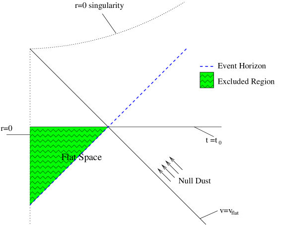
Figure 4: A spacetime diagram of the collapse of null dust in flat space. The coordinate $t$ is such that $(\frac{\partial}{\partial t})^{a}$ is pointing upwards in the flat region in the diagram. The surfaces $v=v_{\text{flat}}$ and $t=t_{0}$ are shown. The excluded region is the region inside the event horizon satisfying $t<t_{0}$. This is the shaded triangular region in the diagram. It follows from the proposition that trapped surfaces cannot extend into this region. As a result, the boundary of the region containing trapped surfaces, is not, in general, the event horizon.

Proposition: Consider a Vaidya spacetime with metric as in (1) such that $R(v)$ is a non-negative, non-decreasing, bounded function, and such that $R(v)=0$ for $v\leq v_{\text{flat}}$ and $R(v)>0$ for $v>v_{\text{flat}}$. Let $t$ be the global inertial time coordinate in the flat region such that the 2-spheres of the global spherical symmetry of the Vaidya spacetime are at rest. Let $t_{0}$ be the value of $t$ at the intersection of the event horizon with the surface $v=v_{0}$. Then, no trapped surface in this spacetime may contain a point with $v<v_{0}$ and $t<t_{0}$.

Proof: Let $U$ be the region in this spacetime that contains all the points that lie inside, or coincide with, the event horizon and with $t\leq t_{0}$. Thus, in the figure, this is the shaded region including the portion of the 3-surface $t=t_{0}$ at the top of the region, and including the portion of the event horizon at the bottom of this region. The region $U$ is compact.

Assume that a trapped surface contains some point $(t_{1},x_{1},y_{1},z_{1})$ that lies strictly inside this region, i.e. $t_{1}<t_{0}$, and, of course, it is strictly inside the event horizon. Let $W$ be the intersection of the trapped surface with $U$. The region $W$ is compact and it is non-empty, since, by assumption, it contains the point above. As a result a minimum for $t$ exists in $W$. Let $(\tilde{t},\tilde{x},\tilde{y},\tilde{z})$ be a point in $W$ where this minimum for $t$ is attained.

This point cannot lie in the boundary of $U$, since this would mean that either $\tilde{t}=t_{0}$ or that the point lies in the event horizon. The first is impossible, since, by assumption, another point in $W$ satisfies $t_{1}<t_{0}$, and therefore this would contradict this point being a minimum for $t$ in $W$. The second is impossible, since trapped surfaces lie strictly inside the event horizon, so the point cannot lie on the event horizon. Therefore, the minimum for $t$ is attained strictly inside $U$, and this implies that $(\tilde{t},\tilde{x},\tilde{y},\tilde{z})$ must be a local minimum for $t$.

Without loss of generality, the Cartesian coordinates can be chosen so that at $(\tilde{t},\tilde{x},\tilde{y},\tilde{z})$, the $z$-axis is orthogonal to the trapped surface. It follows that in a neighborhood of this point, the 2-surface can be expressed in terms of $x$ and $y$. Therefore, in a neighborhood of this point the surface’s coordinates are given by

$$\Big{(}T(x,y),x,y,Z(x,y)\Big{)}$$ (53)

with $T(x,y)$ and $Z(x,y)$ some smooth functions in this neighborhood. Since $(\tilde{t},\tilde{x},\tilde{y},\tilde{z})$ is a local minimum for $t$ then

$$\frac{\partial T(x,y)}{\partial x}|_{(\tilde{x},\tilde{y})}=0\quad\quad\text{and}\quad\quad\frac{\partial T(x,y)}{\partial y}|_{(\tilde{x},\tilde{y})}=0$$ (54)

Similarly, since the $z$-axis is orthogonal to the 2-surface at this point then

$$\frac{\partial Z(x,y)}{\partial x}|_{(\tilde{x},\tilde{y})}=0\quad\quad\text{and}\quad\quad\frac{\partial Z(x,y)}{\partial y}|_{(\tilde{x},\tilde{y})}=0$$ (55)

Consider the 3-surface given by $t-T(x,y)=0$. At $(\tilde{t},\tilde{x},\tilde{y},\tilde{z})$, the normal to the surface, $\nabla_{a}\Big{(}t-T(x,y)\Big{)}$, is timelike. Since this gradient is smooth in the coordinates, then it is timelike in some small neighborhood of $(\tilde{t},\tilde{x},\tilde{y},\tilde{z})$. Furthermore, in this neighborhood the 2-surface given by (53) is embedded in this 3-surface. Consider the sum of the outgoing and ingoing expansions at the point $(\tilde{t},\tilde{x},\tilde{y},\tilde{z})$. Since, in the interchange of ingoing and outgoing, $s^{a}$ changes sign in (52), then in this sum only the first two terms of (52) will contribute. These two terms depend on $t^{a}$, the future directed timelike unit normal to the 3-surface, in a neighborhood of the point. They depend on $s^{a}$, the spacelike unit normal to the 2-surface in the 3-surface, as well as on $h^{ab}$, the metric on the 3-surface. However, in order to evaluate the sum of the expansions at $(\tilde{t},\tilde{x},\tilde{y},\tilde{z})$, $s^{a}$ and $h^{ab}$ are needed only at that point.

A simple evaluation shows that

$$t^{a} = \frac{1}{\sqrt{1-T_{x}^{\ 2}-T_{y}^{\ 2}}}\ (\frac{\partial}{\partial t})^{a}$$ (56)

$$+ \frac{T_{x}}{\sqrt{1-T_{x}^{\ 2}-T_{y}^{\ 2}}}\ (\frac{\partial}{\partial x})^{a}+\frac{T_{y}}{\sqrt{1-T_{x}^{\ 2}-T_{y}^{\ 2}}}\ (\frac{\partial}{\partial y})^{a}$$

where $T_{x}\equiv\frac{\partial T(x,y)}{\partial x}$ and similarly for $T_{y}$. At $(\tilde{t},\tilde{x},\tilde{y},\tilde{z})$, using (54), the metric of the 3-surface is given by

$$h_{ab}|_{\big{(}\tilde{x},\tilde{y},Z(\tilde{x},\tilde{y})\big{)}}=dx_{a}dx_{b}+dy_{a}dy_{b}+dz_{a}dz_{b}$$ (57)

Finally, using (54) and (55), the normal to the 2-surface in the 3-surface at $(\tilde{t},\tilde{x},\tilde{y},\tilde{z})$ is given by

$$s^{a}|_{(\tilde{x},\tilde{y})}=(\frac{\partial}{\partial z})^{a}$$ (58)

It is now possible to use (52) to evaluate the sum of the two expansions. Using $t^{a}$, $h_{ab}$, and $s^{a}$ as above, as well as (54), the sum of the two expansions is found to be

$$\big{(}\Theta_{1}+\Theta_{2}\big{)}|_{(\tilde{t},\tilde{x},\tilde{y},\tilde{z})}=2(\frac{\partial^{2}T(x,y)}{\partial x^{2}}+\frac{\partial^{2}T(x,y)}{\partial y^{2}})$$ (59)

Since the 2-surface is trapped, then the sum of the two expansions is negative, and therefore at least one of the two terms in (59) must be negative. This is a contradiction to $(\tilde{t},\tilde{x},\tilde{y},\tilde{z})$ being a local minimum. (It also shows that for a surface to be trapped, it has to “bend down in time” everywhere in the flat region.)

Thus, the assumption that $(t_{1},x_{1},y_{1},z_{1})$, a point of the trapped surface, lies strictly inside $U$, cannot hold. This completes the proof.

5 Discussion

In Vaidya spacetimes, the situation regarding outer trapped surfaces, is now clear. Outer trapped surfaces can reach arbitrarily close the the event horizon everywhere and Eardley’s conjecture is true for these spacetimes.

Extending the main result to other spacetimes using a similar procedure, seems unlikely since the technique used here relies on precise control of the location of the integral curve relative to the spherically symmetric apparent 3-horizon and the event horizon. The level of precision, required for this particular method, can be obtained in Vaidya spacetimes in the ingoing Eddington-Finkelstein coordinates, but appears to be substantially harder to obtain in general spherically symmetric spacetimes and much more so in spacetimes that are not spherically symmetric. Nonetheless, the class of spacetimes covered by the main result is wide as it includes spacetimes that start flat and later, with some collapsing matter, form a black hole. As a result, since it was shown that outer trapped surfaces exist even in the flat region in such spacetimes, then this appears to, perhaps, capture the essential features of general black hole collapse spacetimes. This then strengthens the expectation that Eardley’s conjecture is true, in general.

The situation regarding trapped surfaces in Vaidya spacetimes was explored as well. A proposition was proved, showing that there is a portion of the flat region of a Vaidya spacetime that is excluded, i.e. that trapped surfaces cannot enter this region. This is consistent with the results of Schnetter and Krishnan [6]. They describe finding a marginally trapped surface that extends into the flat region of a Vaidya spacetime. Since the flat region is not excluded entirely, it follows that the surface described by Schnetter and Krishnan can extend into the flat region in the non-excluded part.

It would be of interest to find in Vaidya spacetimes the exact location of the boundary of the region containing trapped surfaces, as this will give a better understanding of where can surfaces such as future trapping horizons and dynamical horizons be located in these spacetimes. In Fig. 4, this boundary must lie somewhere above the $t=t_{0}$ surface.

Acknowledgments

I am greatly indebted to my advisor, Bob Wald, for many useful discussions and guidance along the way. I have also benefited from discussions with Akihiro Ishibashi. This research was supported in part by NSF grant PHY-0456619 to the University of Chicago. Submitted in partial fulfillment of the requirements of the degree of Doctor of Philosophy, University of Chicago, Chicago, Illinois.

References

- [1] S. W. Hawking and G.F.R. Ellis, Large scale structure of spacetime (Cambridge University Press, Cambridge, 1972).
- [2] S. A. Hayward, Phys. Rev. D 49, 6467 (1994).
- [3] A. Ashtekar and B. Krishnan, Phys. Rev. D 68, 104030 (2003).
- [4] A. Ashtekar and G. Galloway, Adv. Theor. Math. Phys. 9, 1-30 (2005).
- [5] D. M. Eardley, Phys. Rev. D 57, 2299 (1998).
- [6] E. Schnetter and B. Krishnan, Phys. Rev. D 73, 021502(R) (2006).