Comment on “Quantization of FRW spacetimes
in the presence of a cosmological constant and radiation”

Abstract

The quantization of the Friedmann-Robertson-Walker spacetime in the presence of a negative cosmological constant was used in a recent paper to conclude that there are solutions that avoid singularities (big bang–big crunch) at the quantum level. We show that a proper study of their model does not indicate the it prevents the occurrence of singularities at the quantum level, in fact the quantum probability of such event is larger than the classical one. Our numerical simulations based on the powerful variational sinc collocation method (VSCM) also show that the precision of the results of that paper is much lower than the $20$ significant digits reported by the authors.

We review the results presented in a recent paper on Quantum Cosmology by Monerat et al MCOFL06 , concerning the quantization of the Friedmann-Robertson-Walker spacetime. The quantum dynamics of this model is described by the Wheeler-De Witt equation, which is obtained by applying the Dirac formalism to the quantization of constrained systems. Such equation reads

$$\left(\frac{1}{12}\frac{\partial^{2}}{\partial a^{2}}-3ka^{2}+\Lambda a^{4}\right)\Psi(a,\tau)=-i\frac{\partial}{\partial\tau}\Psi(a,\tau)\ ,$$ (1)

and it is formally equivalent to the Schrödinger equation for a quartic anharmonic oscillator with a potential given by MCOFL06

$$V_{e}(a)=36ka^{2}-12\Lambda a^{4}\ .$$ (2)

Here $a$ is the scale factor in the FRW metric, $\Lambda$ is the (negative) cosmological constant and $k$ denotes the constant curvature of the spatial sections.

The corresponding time–independent Schrödinger equation then reads

$$\left(-\frac{\partial^{2}}{\partial a^{2}}+V_{e}(a)\right)\eta(a)=12E\eta(a),$$ (3)

in the notation of Monerat et al MCOFL06 . In what follows we write $\varepsilon\equiv 12\ E$.

Our critique of the arguments of Monerat et al MCOFL06 is based on both technical and conceptual grounds. The former stems from the numerical results obtained in their paper which are below the claimed accuracy. The latter concerns the correct interpretation of the model which does not support the conclusion that singularities are avoided at a quantum level MCOFL06 .

Regarding the technical part, Monerat et al MCOFL06 obtained their results by means of a technique developed by Chhajlany and Malnev CM90 ; CM91 . The application of this method requires the introduction of an extra term in the Schrödinger equation, in the form of a sextic potential with a coefficient obtained from a cubic algebraic equation. Due to this fact the energies and wave functions calculated by Monerat et al are only approximations with roughly $1\%$ error. However, the results reported in Table I of Ref. MCOFL06 , which are obtained using the modified potentials given in their equations (26), (30) and (32) are claimed to have $20$ digits accuracy. Long time ago Fernández FMF91 noticed that the method of Chhajlany et al CM90 ; CM91 converges rather slowly and it therefore requires a much larger number of terms to reach that precision.

In order to verify the accuracy of the results we have used the powerful “Variational Sinc Collocation Method” (VSCM) Amore06a ; Amore06b , which allows one to obtain very precise numerical results, both for the energies and wavefunctions, and has proved to yield errors that decay exponentially with the number of elements (sinc functions) used.

In what follows we briefly sketch the VSCM. The sinc functions are given by

$$S_{k}(h,x) \equiv \frac{\sin\left(\pi(x-kh)/h\right)}{\pi(x-kh)/h}\ ,$$ (4)

where $k=0,\pm 1,\dots$ is an integer and $h$ is the spacing between two contiguous sinc functions. The sinc functions are orthogonal:

$$\int_{-\infty}^{+\infty}S_{k}(h,x)\ S_{l}(h,x)\ dx=h\ \delta_{kl}.$$ (5)

Using a collocation scheme, one can express the matrix element of the Hamiltonian operator in the sinc “basis” as

$$H_{kl}\approx h\left[-c_{kl}^{(2)}+\delta_{kl}\ V(kh)\right]\ ,$$ (6)

where

$$c_{lk}^{(2)} \equiv \left\{\begin{array}[]{c}-\frac{\pi^{2}}{3h^{2}}\ \ if\ \ k=l\\ -\frac{2}{h^{2}}\frac{(-1)^{k-l}}{(k-l)^{2}}\ \ if\ \ k\neq l\end{array}\right.$$ (9)

are the coefficients obtained from the discretization of the second derivative. Diagonalization of the $N\times N$ matrix yields a set of $N$ eigenvalues (energies) and eigenvectors (wavefunctions). Notice however, that the diagonalization of $H$ requires the specification of the otherwise arbitrary grid spacing $h$. For a given number $N$ of sinc functions there exists an optimal value of $h$ which provides the smallest errors. As shown by Amore and collaborators Amore06a ; Amore06b such optimal value of $h$ can be found by application of the Principle of Minimal Sensitivity (PMS) Ste81 to the trace of the $N\times N$ hamiltonian matrix. Notice that once the hamiltonian matrix has been diagonalized one can also solve the time–dependent Schrödinger equation, in terms of the stationary states previously calculated.

Our table 1 shows the odd energies for the potentials given in equations (26), (30) and (32) of Ref. MCOFL06 using the VSCM. The results in this table are correct up to the $20^{th}$ digit, and show that the results reported by Monerat et al in their Table I MCOFL06 are considerably less precise than they appear to suggest. Just to mention one example, their energy $E_{16}$ corresponding to $k=1$ has just $5$ correct digits. Although this lack of precision does not affect the authors’ analysis MCOFL06 , which is in any case bounded by the more severe $1\%$ error due to the use of an effective potential rather than the exact one, we believe that it is important to remark this point.

Table 1: Lowest energy levels for the effective potentials with $k=0,\pm 1$.

Level	$k=1$	$k=0$	$k=-1$
$E_{1}$	$1.5103016760578707333$	$0.3404027974289474964$	$-10.553138375809812184$
$E_{2}$	$3.5509871014722926520$	$1.0496018816142096406$	$-8.8509608822646650503$
$E_{3}$	$5.6230931685079239340$	$1.9248782225982734499$	$-7.2247835560429854525$
$E_{4}$	$7.7256531719676264015$	$2.9232145294809850623$	$-5.6802949920840011967$
$E_{5}$	$9.8577817763092210058$	$4.0227383298745516995$	$-4.2251989178977204001$
$E_{6}$	$12.018664366203979043$	$5.2097960735587976352$	$-2.8707515711793779600$
$E_{7}$	$14.207548236413247839$	$6.4748734068112171253$	$-1.6348253113363418720$
$E_{8}$	$16.423735233636153025$	$7.8108774875618647285$	$-0.5364307199618285749$
$E_{9}$	$18.666575557925837760$	$9.2122719234208330574$	$0.481759254997070592451$
$E_{10}$	$20.935462499941518896$	$10.674588220211030332$	$1.583190805382159479497$
$E_{11}$	$23.229827940734217332$	$12.194126732921328651$	$2.833031712002511140698$
$E_{12}$	$25.549138478317595566$	$13.767762283584094708$	$4.213983702088123106309$
$E_{13}$	$27.892892073596735435$	$15.392811775837602761$	$5.707834132050646278314$
$E_{14}$	$30.260615129836301427$	$17.066940597587263816$	$7.302868225546844668469$
$E_{15}$	$32.651859936513780000$	$18.788094386112582846$	$8.990905434198164180404$
$E_{16}$	$35.066202421382313215$	$20.554447991460572182$	$10.76576537713456435413$
$E_{17}$	$37.503240164769059826$	$22.364366463785281446$	$12.62252647249543208197$
$E_{18}$	$39.962590638221848703$	$24.216374668801875820$	$14.55712323817216360861$
$E_{19}$	$42.443889636078437368$	$26.109133235245860851$	$16.56610649829916492072$
$E_{20}$	$44.946789873733933173$	$28.041419241199542663$	$18.64649041909474222481$
$E_{21}$	$47.470959730597782399$	$30.012110508653406479$	$20.79564954975016308111$
$E_{22}$	$50.016082119171135490$	$32.020172687758339925$	$23.01124646297271199397$
$E_{23}$	$52.581853464498535137$	$34.064648527576543759$	$25.29117906504417774373$

Table 2: Lowest energy levels for the exact potential with $k=0,\pm 1$.

Level	$k=1$	$k=0$	$k=-1$
$E_{1}$	$1.5102625384705021518$	$0.3364795921008755186$	$-21.79569603947057798056$
$E_{2}$	$3.5506472908620463050$	$1.0311990503013958552$	$-20.39848968823294656013$
$E_{3}$	$5.6218937064348010503$	$1.8807615814216099958$	$-19.01885125967730517826$
$E_{4}$	$7.7227778139934265020$	$2.8424874930254863943$	$-17.65745105165687339198$
$E_{5}$	$9.8521942203839334149$	$3.8947462112216761884$	$-16.31503013488920386315$
$E_{6}$	$12.009138568080285499$	$5.0240915609641800702$	$-14.99241327017434870429$
$E_{7}$	$14.192693387434484198$	$6.2211924298081547999$	$-13.69052532294706014390$
$E_{8}$	$16.402016547726087957$	$7.4791208557098708821$	$-12.41041248037188872561$
$E_{9}$	$18.636331727173164959$	$8.7924907241645713076$	$-11.15327022078174141020$
$E_{10}$	$20.894920472196314023$	$10.156971843165374589$	$-9.920481041305256697868$
$E_{11}$	$23.177115522582541829$	$11.568992820956286787$	$-8.713666752230586250096$
$E_{12}$	$25.482295155850129982$	$13.025548149708503746$	$-7.534763378250629251892$
$E_{13}$	$27.809878360230719403$	$14.524066967082505523$	$-6.386132854421764354442$
$E_{14}$	$30.159320687349375640$	$16.062320376957969417$	$-5.270738293115111860300$
$E_{15}$	$32.530110667020528246$	$17.638353963148189178$	$-4.192437789021558602284$
$E_{16}$	$34.921766690427654626$	$19.250437372785090866$	$-3.156519423136907030485$
$E_{17}$	$37.333834286304756785$	$20.897025823964631886$	$-2.170719224552462670164$
$E_{18}$	$39.765883728998739663$	$22.576730162849598220$	$-1.246288323062400948910$
$E_{19}$	$42.217507928478425449$	$24.288293189747778350$	$-0.389996330189812857692$
$E_{20}$	$44.688320561206965683$	$26.030570672865707451$	$0.433719867112653240009$
$E_{21}$	$47.177954407853964266$	$27.802515928224750562$	$1.300741393435948191383$
$E_{22}$	$49.686059869496678687$	$29.603167154324565317$	$2.243855389930394850590$
$E_{23}$	$52.212303638550624930$	$31.431636924008847119$	$3.256001768433707607172$

We wish to stress that the numerical method that we have used is completely general and can be applied to arbitrary potentials; for this reason we have decided to perform the numerical simulation and time evolution of the model with the exact potential, rather than following the strategy of Monerat et al MCOFL06 , which was dictated by their choice of numerical method CM90 ; CM91 . Table 2 shows the eigenvalues corresponding to the exact potential Eq. (2). Particularly in the case $k=-1$, corresponding to a double well we have verified that the results are quite different from the ones obtained with the effective potential (compare the fourth columns of tables 1 and 2).

By means of the VSCM we have obtained accurate energies $E_{n}$ and wavefunctions $\phi_{n}(a)$ up to $n=23$. Using these states we can build a wave packet

$$\Theta(a,\tau)=\sum_{n}B_{n}\phi_{n}(a)\ e^{-i\varepsilon_{n}\tau}$$ (10)

where the coefficients $B_{n}$ are taken to be equal to unity as in Ref. MCOFL06 and the energies $\varepsilon_{n}=12E_{n}$. The expected value of the scale factor is

$$\langle a\rangle=\frac{\int_{0}^{\infty}a\ |\Theta(a,\tau)|^{2}da}{\int_{0}^{\infty}|\Theta(a,\tau)|^{2}da}=\frac{\sum_{nn^{\prime}}B_{n}^{*}B_{n^{\prime}}\kappa_{nn^{\prime}}e^{i(\varepsilon_{n}-\varepsilon_{n^{\prime}})\tau}}{\sum_{n}|B_{n}|^{2}},$$ (11)

where $\kappa_{nn^{\prime}}\equiv\int_{0}^{\infty}a\ \phi_{n}^{*}(a)\phi_{n^{\prime}}(a)da$. This expectation value oscillates in time because of the time–dependent terms $e^{i(\varepsilon_{n}-\varepsilon_{n^{\prime}})t}$. Likewise the energy of the wave packet is ${\cal E}_{wp}=\sum_{n}|B_{n}|^{2}\varepsilon_{n}/\sum_{n}|B_{n}|^{2}$.

We notice that the wave packet of eq. (10) is not yet fully specified, since the eigenfunctions $\phi_{n}(a)$ are known up to a phase factor which can be chosen arbitrarily. By looking at the coefficients in Table II of MCOFL06 and of Tables II-VII of MCOFL06arxiv we see that these wave functions have been chosen by Monerat and collaborators to be positive in a small neighborhood of $a=0^{+}$. The wave packet obtained with this prescription for $k=1$ corresponds at $t=0$ to a state sharply localized around $a=0.1$, which quickly spreads at later times according to the Heisenberg principle. The reader can look at the left plot in Fig. 1, where the wave packet at $t=0$ and $t=10$ is plotted . The wave packet for $k=-1$ is plotted in the right plot of Fig. 1.

Fig.1 of MCOFL06 displays the expectation value of the scale factor for $\Lambda=-0.1$ and $k=1$; in this plot it is difficult to appreciate the localization of the wave packet, since the curve is compressed by the large time scale considered. In fig.2 of the present paper we show the behavior of the expectation value $\langle a\rangle$ for $\Lambda=-0.1$ and $k=\pm 1$ using the same choice of phases of Monerat et al. Our result for $k=1$ is similar to the one observed by Monerat et al.: the expectation value of the scale factor starts at $a\approx 0.1$ at $t=0$ and then strongly oscillates at later times, in accordance with the Heisenberg principle; for $k=-1$, however, our curve is different from the corresponding curve of Fig.3 of MCOFL06 , and $\langle a\rangle$ oscillates around a larger value. The reason for this discrepancy is the poor accuracy of the results of Monerat et al. especially for the case $k=-1$: the fact that $\langle a\rangle$ oscillates around $a\approx 3$ in our figure reflects both the incorrectness of the eigenfunctions calculated in MCOFL06 and the presence of a minimum of the potential at $a=\sqrt{\frac{3k}{2\Lambda}}=\sqrt{15}$ (being the energy of the wave packet negative).

The dashed horizontal lines in our figure correspond to the classical expectation value $\langle a\rangle_{cl}$ for a particle moving in the same potential and with the same energy of the wave packet. The classical probability of finding a given value for the scale factor is given by

$$P_{cl}(a)=\frac{N_{cl}}{\sqrt{V(a_{+})-V(a)}}$$ (12)

where $N_{cl}=1/\int_{0}^{a_{+}}\frac{da}{\sqrt{V(a_{+})-V(a)}}$ and $a_{+}$ is the right inversion point (remember that in our problem there is an infinite wall at the origin) given by ${\cal E}_{wp}=V(a_{+})$.

Based on the behavior of $\langle a\rangle$ in their figures 1-3 the authors of MCOFL06 state that they “may be confident about all values assumed by $\langle a\rangle$, in particular, that it does not vanish”, thus concluding that this proves the absence of a big-crunch in the model at the quantum level or using their own words “since the expectation values of the scale factors never vanish, we have an initial indication that these models may not have singularities at the quantum level”.

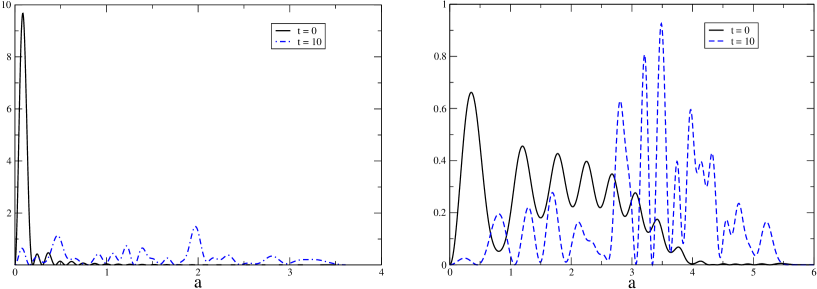
Figure 1: Wave packets for $\Lambda=-0.1$ and $k=1$ (left plot) and $k=-1$ (right plot) at two different times. (color online)

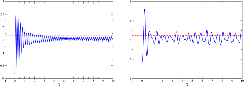
Figure 2: Behavior of the expectation value $\langle a\rangle$ for $\Lambda=-0.1$ and $k=1$ (left plot) and $k=-1$ (right plot). (color online)

In our opinion these observations are not correct: in the first place, one concludes that $\langle a\rangle\neq 0$ without any calculation because it is a consequence of the presence of an infinite wall located at $a=0$ and is therefore completely independent of the form of the potential. In the second place, and more importantly, the condition $\langle a\rangle\neq 0$ does not imply the absence of a big crunch and actually holds even at the classical level. As a matter of fact, simple mathematical considerations, based on the form of $P_{cl}(a)$, are sufficient to conclude that $\langle a\rangle_{cl}>0$ . As we have said the horizontal curves in Fig. 2 correspond to the classical expectation values which in both cases fall in the region of oscillation of the quantum expectation value. For this reason we believe that hardly any conclusion can be drawn from the study of $\langle a\rangle$ performed in Fig.1-3 of MCOFL06 .

We also stress that, although the expectation value of the scale factor can never vanish, one can build wave packets which at a given time (say $t=0$) are localized around an arbitrarily small values, $a_{0}$. Such wave packets are obtained using $B_{n}=\phi_{n}^{*}(a_{0})$ for the first $N$ states of the potential using the completeness of the basis $\left\{\phi_{n}(a)\right\}$:

$$\delta(a-a_{0})\approx\sum_{n=0}^{N}\phi^{*}_{n}(a_{0})\phi_{n}(a)\ .$$ (13)

On the other hand, a more meaningful comparison between the classical and quantum cases can be made by calculating the probability of finding $a$ in a region between $0$ and $a_{max}$. Fig. 3 shows the quantum probability that the scale factor is smaller than a given value $a$ at three different times, for the wave packet with $B_{n}=1$, and $k=\pm 1$ (left and right plot respectively) and also its classical analogue (solid line), using the same phase convention of MCOFL06 . We have used a logarithmic scale in the plots to better appreciate the region around $a=0$.

For $k=1$ we see that at $t=0$ the quantum probability differs strongly from the classical one, since the scale factor is localized around $a\approx 0.1$, while at later times when the packet spreads, the quantum probability gets closer to its classical counterpart. At $t=0$ only for quite small values of $a$ the classical probability is larger than the quantum one, as a consequence of the Dirichlet boundary conditions on the wave functions.

More dramatic differences are observed for $k=-1$: in this case the region around $a=0$ is classically forbidden and only the quantum probability is nonvanishing around $a=0$.

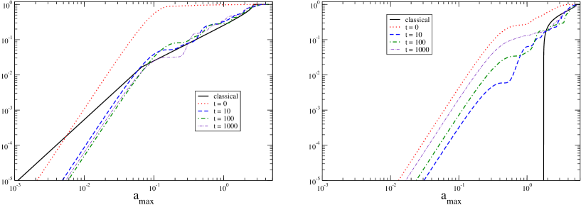
Figure 3: Probability of finding a scale factor $\leq a$ for $\Lambda=-0.1$ and $k=1$ (left plot) and $k=-1$ (right plot). (color online)

Concluding, we feel that the question posed in MCOFL06 , whether in the quantum model the singularity is avoided, has not been addressed properly in that paper : the observation that $\langle a\rangle>0$ is trivial and holds both at classical and quantum level; The expectation values calculated for the wave packets considered in MCOFL06 oscillate around the corresponding classical expectation values and can never vanish neither in classical or in quantum mechanics. The strong oscillations observed for the case $k=1$ are understood as a consequence of the Heisenberg principle.

On the other hand, we feel that a better tool to address the question posed by Monerat et al. is to calculate the probability of finding a scale factor below a given value (such tool was not considered in MCOFL06 ). Our result show that only for very small $a$ the classical probability is larger than the quantum one, although this effect is a mere consequence of the Dirichlet boundary conditions, and therefore holds regardless of the binding potential used (in this case a quartic potential).

References

• (1) G. A. Monerat, E. V. Corrêa Silva, G. Oliveira–Neto, L. G. Ferreira Filho, and N. A. Lemos, Phys. Rev. D 33, 044022 (2006)
• (2) G. A. Monerat, E. V. Corrêa Silva, G. Oliveira–Neto, L. G. Ferreira Filho, and N. A. Lemos, gr-qc/0508086
• (3) S. C. Chhajlany and V. N. Malnev, Phys. Rev. A 42, 3111 (1990)
• (4) S. C. Chhajlany, D. A. Letov and V. N. Malnev, J. Phys. A 24, 2731 (1991)
• (5) F. M. Fernándenz, Phys. Rev. A 44, 3336-3339 (1991)
• (6) P. Amore, Journal of Physics A 39, L349-L355 (2006)
• (7) P. Amore, M. Cervantes and F. M. Fernández , submitted to J. Phys. A (2006)
• (8) P. M. Stevenson, Phys. Rev. D 23, 2916 (1981).