An Extensive Search for Overtones in Schwarzschild Black Holes

Abstract

In this paper we show that with standard methods it is possible to obtain highly precise results for QNMs. In particular, secondary modes are obtained by numerical integration. We compare several results making a detailed analysis.

I Introduction

Wave propagation around black holes is an active field of research (see Regge-57 ). The perspective of gravitational waves detection in a near future and the great development of numerical general relativity have increased even further the activity on this field aguiar . Gravitational waves should be especially strong when emitted by black holes. The study of the propagation of perturbations around them is, hence, essential to provide templates for the gravitational waves identification. Thus, activity in this field is developping quickly many .

The Schwarzschild black hole is rather well known Regge-57 ; Konoplya but it is important to get reassured about the robustness of the methods and results. Therefore, here, we embark in a detailed study of the secondary modes by means of the subtraction of the first modes in time domain. The method, though very simple has not been used in the literature due to numerical errors implicit in the method. However, we were able to use simple standard methods to show that the results are valid implying an acuracy of seven figures for the dominant mode and sometimes three for the secondary one.

We have used the geometric system of units, for which $\hbar=c=G=1$. This means that the masses have dimension of length and are measured in metres. The conversion factor from metres to kilograms is $c^{2}/G$.

II Fundamental Modes and First Overtones

We begin with a series of tables on the frequencies of the QNMs for the Schwarzschild black holes. We have employed, throughout our discussion, $M=1.0m$ since the black-hole frequencies scales as $M\omega=const$. For the grid spacing, we have used $h=10^{-2}m$. In what follows, we have used the notation $\omega^{DOM}$ for the dominant mode, $\omega^{SEC}$ for the first overtone and, whenever applicable, $\omega^{TER}$ for the second overtone.

$\ell$	$\omega_{DOM}$	$\delta\omega_{DOM}$	$\omega_{SEC}$	$\omega_{TER}$
$1$	$-$	$-$	$-$	$-$
$2$	$0.483644-0.0967590i$	$3E-7$	$0.470-0.300i$	$-$
$3$	$0.675367-0.0964997i$	$2E-7$	$0.667-0.288i$	$-$
$4$	$0.867417-0.0963923i$	$2E-7$	$0.859-0.287i$	$-$
$5$	$1.059614-0.0966337i$	$6E-7$	$1.050-0.283i$	$-$
$6$	$1.251891-0.0963060i$	$9E-8$	$1.224-0.283i$	$-$
$7$	$1.444214-0.0962866i$	$7E-7$	$1.433-0.282i$	$-$
$8$	$1.636565-0.0962724i$	$1E-6$	$1.629-0.288i$	$1.584-0.422i$
$9$	$1.828959-0.0962639i$	$1E-6$	$1.822-0.288i$	$1.791-0.404i$
$10$	$2.021329-0.0962568i$	$1E-6$	$2.014-0.288i$	$1.990-0.405i$
$11$	$2.213730-0.0962522i$	$1E-6$	$2.207-0.288i$	$2.174-0.440i$
$12$	$2.406139-0.0962487i$	$1E-6$	$2.400-0.288i$	$2.371-0.440i$

Table 1: Frequencies for the Schwarzschild BH of $M=1.0m$. Scalar Field, different $\ell$ values.

$\ell$	$\omega_{DOM}$	$\delta\omega_{DOM}$	$\omega_{SEC}$	$\omega_{TER}$
$1$	$0.248229-0.0924905i$	$-$	$-$	$-$
$2$	$0.457595-0.0950044i$	$5E-8$	$0.440-0.290i$	$-$
$3$	$0.656899-0.0956165i$	$2E-8$	$0.648-0.286i$	$-$
$4$	$0.853096-0.0958605i$	$2E-7$	$0.844-0.285i$	$-$
$5$	$1.047915-0.0959821i$	$9E-8$	$1.039-0.282i$	$-$
$6$	$1.242000-0.0960523i$	$9E-8$	$1.232-0.282i$	$-$
$7$	$1.435647-0.0960959i$	$7E-7$	$1.424-0.281i$	$-$
$8$	$1.629012-0.0961250i$	$6E-8$	$1.621-0.288i$	$1.577-0.425i$
$9$	$1.822180-0.0961452i$	$1E-6$	$1.815-0.288i$	$1.788-0.407i$
$10$	$2.015214-0.0961596i$	$1E-6$	$2.008-0.288i$	$1.984-0.410i$
$11$	$2.208148-0.0961714i$	$2E-6$	$2.199-0.285i$	$2.164-0.442i$
$12$	$2.401004-0.0961800i$	$1E-6$	$2.395-0.288i$	$2.365-0.427i$

Table 2: Frequencies for the Schwarzschild BH of $M=1.0m$. Electromagnetic Field, different $\ell$ values.

$\ell$	$\omega_{DOM}$	$\delta\omega_{DOM}$	$\omega_{SEC}$	$\omega_{TER}$
$2$	$0.37367-0.08896i$	$6E-6$	$0.352-0.271i$	$-$
$3$	$0.599444-0.0927031i$	$5E-9$	$0.586-0.278i$	$-$
$4$	$0.809180-0.0941643i$	$4E-8$	$0.797-0.279i$	$-$
$5$	$1.012297-0.0948713i$	$3E-7$	$1.002-0.279i$	$-$
$6$	$1.212013-0.0952667i$	$2E-7$	$1.203-0.286i$	$-$
$7$	$1.409741-0.0955106i$	$2E-7$	$1.401-0.286i$	$1.361-0.432i$
$8$	$1.606202-0.0956724i$	$3E-7$	$1.594-0.280i$	$1.474-0.515i$
$9$	$1.801801-0.0957836i$	$1E-6$	$1.795-0.287i$	$1.770-0.411i$
$10$	$1.996796-0.0958649i$	$2E-7$	$1.990-0.286i$	$1.967-0.408i$
$11$	$2.191345-0.0959263i$	$2E-7$	$2.188-0.287i$	$2.154-0.415i$
$12$	$2.385555-0.0959724i$	$2E-7$	$2.379-0.287i$	$2.353-0.446i$

Table 3: Frequencies for the Schwarzschild BH of mass $M=1.0m$. Axial Field, different $\ell$ values.

A few remarks are due: the scalar $\ell=0$ field oscillated almost nothing, so no frequencies were computed for it at all. The second overtone wasn’t clearly visible for $\ell<6$, and even so only for $\ell=8$ and higher we could make minimally acceptable fittings to it.

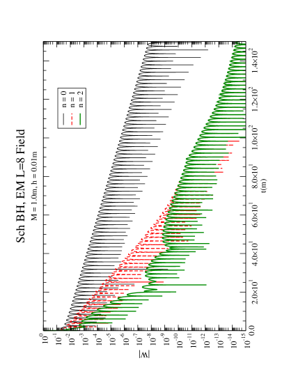
Figure 1: Fundamental mode and first overtone, for the electromagnetic $\ell=8$ field. The second overtone is much clearer than in the previous figures.

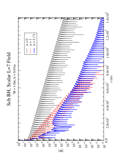
Figure 2: Fundamental mode and first overtone, for the scalar $\ell=7$ field. The second overtone also appears, though not in a very evident manner.

The figures (1) and (2) show that the second overtone appears clearly only for very high $\ell$ ($\ell>6$), and it is the reason why we have blank spaces for this overtone in tables (1) and (2).

We have compared our data to those generated via 6th-order WKB computations, from Konoplya and 3rd-order WKB from Iyer-87 . When it comes to notation, we have employed $\ell$ for the multipole index (as before), $n$ for the overtone index ($n=0$ for the fundamental, $n=1$ for the first overtone, and so on). $\omega_{NUM}$ refers to our numerical data, $\omega_{WKB1}$ refers to the WKB data from paper Konoplya and $\omega_{WKB2}$, to paper Iyer-87 .

$\ell$	$n$	$\omega_{NUM}$	$\omega_{WKB1}$	$\omega_{WKB2}$
$0$	$0$	$-$	$0.1105-0.1008i$	$0.1046-0.1152i$
$1$	$0$	$0.292939-0.0976663i$	$0.2929-0.0977i$	$0.2911-0.0980i$
$1$	$1$	$-$	$0.264-0.307i$	$0.2622-0.3074i$
$2$	$0$	$0.483644-0.0967590i$	$0.4836-0.0968i$	$0.4832-0.0968i$
$2$	$1$	$0.470-0.300i$	$0.4638-0.2956i$	$0.4632-0.2958i$
$2$	$2$	$-$	$0.4317-0.5034i$	$0.4317-0.5034i$
$3$	$0$	$0.675367-0.0964997i$	$0.675366-0.0965006i$	$-$
$3$	$1$	$0.667-0.288i$	$0.660671-0.292288i$	$-$
$4$	$0$	$0.867417-0.0963923i$	$0.867416-0.0963919i$	$-$
$4$	$1$	$0.859-0.287i$	$0.855808-0.290877i$	$-$
$5$	$0$	$1.059614-0.0963337i$	$1.05961-0.0963368i$	$-$
$5$	$1$	$1.050-0.283i$	$1.05004-0.290154i$	$-$
$6$	$0$	$1.251891-0.0963060i$	$1.25189-0.0963051i$	$-$
$6$	$1$	$1.224-0.283i$	$1.24375-0.289736i$	$-$
$7$	$0$	$1.444214-0.0962866i$	$1.44421-0.0962852i$	$-$
$7$	$1$	$1.433-0.282i$	$1.43714-0.289473i$	$-$
$8$	$0$	$1.636565-0.0962724i$	$1.63656-0.0962719i$	$-$
$8$	$1$	$1.629-0.288i$	$1.63031-0.289297i$
$8$	$2$	$1.584-0.422i$	$1.61797-0.483757i$
$9$	$0$	$1.828939-0.0962639i$	$1.82893-0.0962626i$	$-$
$9$	$1$	$1.822-0.288i$	$1.82333-0.289173ii$
$9$	$2$	$1.791-0.404i$	$1.81225-0.483235i$
$10$	$0$	$2.021329-0.0962568i$	$2.02132-0.0962558i$	$-$
$10$	$1$	$2.014-0.288i$	$2.01625-0.289083i$
$10$	$2$	$1.990-0.405i$	$2.0062-0.482854i$
$11$	$0$	$2.213730-0.0962522i$	$2.21372-0.0962507i$	$-$
$11$	$1$	$2.207-0.288i$	$2.20909-0.289015i$
$11$	$2$	$2.174-0.417i$	$2.19989-0.482567i$
$12$	$0$	$2.406139-0.0962487i$	$2.40613-0.0962467i$	$-$
$12$	$1$	$2.400-0.288i$	$2.40186-0.288963i$
$12$	$2$	$2.371-0.440i$	$2.39338-0.482347i$

Table 4: Frequencies for the Schwarzschild BH of $M=1.0m$. Scalar Field, different $\ell$ and $n$ values. Comparing to WKB data.

$\ell$	$n$	$\omega_{NUM}$	$\omega_{WKB1}$	$\omega_{WKB2}$
$1$	$0$	$0.248229-0.0924905i$	$0.2482-0.0926i$	$0.2459-0.0931i$
$1$	$1$	$-$	$0.2143-0.2941i$	$0.2113-0.2958i$
$2$	$0$	$0.457595-0.0950044i$	$0.4576-0.0950i$	$0.4571-0.0951i$
$2$	$1$	$0.440-0.290i$	$0.4365-0.2907i$	$0.4358-0.2910i$
$2$	$2$	$-$	$0.4009-0.5017i$	$0.4023-0.4959i$
$3$	$0$	$0.656899-0.0956165i$	$0.6569-0.0956i$	$0.6567-0.0951i$
$3$	$1$	$0.648-0.286i$	$0.6417-0.2897i$	$0.6415-0.2898i$
$3$	$2$	$-$	$0.6138-0.4921i$	$0.6151-0.4901i$
$3$	$3$	$-$	$0.5814-0.6955i$	$0.5814-0.6955i$
$4$	$0$	$0.853096-0.0958605i$	$0.853095-0.0958601i$	$-$
$4$	$1$	$0.844-0.285i$	$0.841267-0.289315i$	$-$
$5$	$0$	$1.047915-0.0959821i$	$1.04791-0.095981i$	$-$
$5$	$1$	$1.039-0.282i$	$1.03822-0.289104i$	$-$
$6$	$0$	$1.242000-0.0960523i$	$1.242-0.0960512i$	$-$
$6$	$1$	$1.232-0.282i$	$1.23379-0.288982i$	$-$
$7$	$0$	$1.435647-0.0960959i$	$1.43564-0.0960947i$	$-$
$7$	$1$	$1.424-0.281i$	$1.42852-0.288906i$	$-$
$8$	$0$	$1.629012-0.0961250i$	$1.629-0.0961236i$	$-$
$8$	$1$	$1.621-0.288i$	$1.62272-0.288855i$	$-$
$8$	$2$	$1.577-0.425i$	$1.61032-0.483028i$	$-$
$9$	$0$	$1.822180-0.0961452i$	$1.82217-0.0961439i$	$-$
$9$	$1$	$1.815-0.288i$	$1.81655-0.288819i$	$-$
$9$	$2$	$1.788-0.407i$	$1.80542-0.48265i$	$-$
$10$	$0$	$2.015214-0.0961596i$	$2.01521-0.0961587i$	$-$
$10$	$1$	$2.006-0.288i$	$2.01012-0.288793i$	$-$
$10$	$2$	$1.984-0.410i$	$2.00003-0.482374i$	$-$
$11$	$0$	$2.208148-0.0961714i$	$2.20814-0.0961697i$	$-$
$11$	$1$	$2.199-0.285i$	$2.20349-0.288773i$	$-$
$11$	$2$	$2.161-0.442i$	$2.19426-0.482167i$	$-$
$12$	$0$	$2.401004-0.096180i$	$2.40099-0.0961782i$	$-$
$12$	$1$	$2.395-0.288i$	$2.39672-0.288758i$	$-$
$12$	$2$	$2.365-0.427i$	$2.38822-0.482007i$	$-$

Table 5: Frequencies for the Schwarzschild BH of $M=1.0m$. Electromagnetic field, different $\ell$ and $n$ values. Comparing to WKB values.

$\ell$	$n$	$\omega_{NUM}$	$\omega_{WKB1}$	$\omega_{WKB2}$
$2$	$0$	$0.37367-0.08896i$	$0.373691-0.088891i$	$0.3732-0.0892i$
$2$	$1$	$0.352-0.272i$	$0.346297-0.27348i$	$0.3460-0.2749i$
$2$	$2$	$-$	$0.2985-0.4776i$	$0.29852-0.47756i$
$3$	$0$	$0.599444-0.0927031i$	$0.599443-0.0927025i$	$0.5993-0.0927i$
$3$	$1$	$0.587-0.278i$	$0.582642-0.28129i$	$0.5824-0.2814i$
$3$	$2$	$-$	$0.551594-0.479047i$	$0.5532-0.4767i$
$4$	$0$	$0.809180-0.0941643i$	$0.809178-0.0941641i$	$0.8091-0.0942i$
$4$	$1$	$0.797-0.279i$	$0.796631-0.284334i$	$0.7965-0.2844i$
$4$	$2$	$-$	$0.7727-0.4799i$	$0.772695-0.4799i$
$5$	$0$	$1.012297-0.0948713i$	$1.0123-0.0948706i$	$-$
$5$	$1$	$1.002-0.279i$	$1.00222-0.285817i$	$-$
$6$	$0$	$1.212013-0.0952667i$	$1.21201-0.0952659i$	$-$
$6$	$1$	$1.203-0.286i$	$1.20357-0.28665i$	$-$
$7$	$0$	$1.409741-0.0955106i$	$1.40974-0.0955096i$	$-$
$7$	$1$	$1.401-0.286i$	$1.40247-0.287164i$	$-$
$7$	$2$	$1.361-0.432i$	$1.38818-0.480709i$	$-$
$8$	$0$	$1.606202-0.0956724i$	$1.60619-0.0956707i$	$-$
$8$	$1$	$1.594-0.280i$	$1.59981-0.287504i$	$-$
$8$	$2$	$1.474-0.515i$	$1.58721-0.480804i$	$-$
$9$	$0$	$1.801801-0.095784i$	$1.80179-0.0957828i$	$-$
$9$	$1$	$1.795-0.288i$	$1.7961-0.287741i$	$-$
$9$	$2$	$1.770-0.440i$	$1.78483-0.48087i$	$-$
$10$	$0$	$1.996796-0.0958649i$	$1.99679-0.0958639i$	$-$
$10$	$1$	$1.990-0.286i$	$1.99165-0.287912i$	$-$
$10$	$2$	$1.967-0.408i$	$1.98145-0.48087i$	$-$
$11$	$0$	$2.191345-0.0959263i$	$2.19133-0.0959245i$	$-$
$11$	$1$	$2.185-0.287i$	$2.18665-0.28804i$	$-$
$11$	$2$	$2.154-0.415i$	$2.17734-0.480952i$	$-$
$12$	$0$	$2.385555-0.0959724i$	$2.38554-0.095971i$	$-$
$12$	$1$	$2.379-0.287i$	$2.38124-0.288138i$	$-$
$12$	$2$	$2.353-0.446i$	$2.37268-0.480979i$	$-$

Table 6: Frequencies for the Schwarzschild BH of mass $M=1.0m$. Axial Field, different $\ell$ and $n$ values. Comparing data to WKB.

These comparison tables leave no room for doubts when it comes to the fundamental mode, $n=0$. For all fields and $\ell$-values, the data from our numerical simulations and those from the 6th-order WKB method showed a high-degree agreement, with differences between 1 part in $10^{4}$ and 1 part in $10^{5}$, for both $Re(\omega)$ and $Im(\omega)$, especially for higher $\ell$-values. When it comes to the first overtone, for all fields under study, the agreement between both sets of data was not so impressive, hovering around $1-2\%$ for $Re(\omega)$ and $2-3\%$ for $Im(\omega)$ for low $\ell$ (typically up to $\ell=6$) and improving for higher $\ell$, to a few parts in 1000 for $Re(\omega)$ and around $0.5\%$ or so for $Im(\omega)$. The second overtone showed much higher discrepancies, especially for $Im(\omega)$, with differences around $15\%$ is some cases, while for $Re(\omega)$ this difference usually hovers around $1-2\%$ (with two exceptions for $\ell=8$, when it was much bigger - almost $8\%$ for the axial field).

Appendix A Finding the Overtones Numerically

A comment is due on the method of extracting the secondary (and, whenever applicable, the tertiary) mode: we took the first (or dominant) mode ($n=0$) and applied an oscillatory fitting to it, in order to extract the data on its oscillatory frequency $\omega_{R}$, amplitude $A$ and decay rate $\omega_{I}$. These data were taken with the maximum number of significant digits possible (usually 8 or 9), and we subtracted the fitted function, which had the form

$$\Psi_{0}=A\exp(i\omega_{R}^{0}t)\exp(-\omega_{I}^{0}t),$$ (1)

so that we could see the remainder of this operation. In all cases (except for the $\ell=0,1$ scalar and $\ell=1$ EM field), we could find a remainder of the form

$$\Psi_{R}=B\exp(i\omega_{R}^{1}t)\exp(-\omega_{I}^{1}t)+\Delta,$$ (2)

in which $\omega_{1}\neq\omega_{0}$, characterizing a secondary mode (the first overtone), and with similar amplitudes ($A\thickapprox B$). The term $\Delta$ is just the $\Psi_{0}$ term, but with a much reduced amplitude, indicating that the fitting operation has its precision limitations. This can be seen in the form of parallel curve envelopes in the figures from above.

A similar procedure was adopted to find the second overtone, this time applying the oscillatory fitting to the first overtone, in which a new remainder similar to that seen in (2) was seen. In this latter case, however, only the very high $\ell$-values could yield any valuable result when an oscillatory fitting was applied to it.

Now it is the time to estimate the precision of the first fitting. As we can see again in the aforementioned figures, there is a given time $t_{c}$ for which the secondary mode and the dominant mode are roughly equal in magnitude, that is

$$B\exp(i\omega_{R}^{1}t)\exp(-\omega_{I}^{1}t)\thickapprox\delta(A\exp(i\omega_{R}^{0}t)\exp(-\omega_{I}t)).$$ (3)

The variation of the dominant mode can be expressed as

$$\delta(A\exp(i\omega_{R}^{0}t)\exp(-\omega_{I}t))=(\delta A)\exp(i\omega_{R}^{0}t)\exp(-\omega_{I}t) +$$ (4)

$$+ Ai\exp(i\omega_{R}t)\exp(-\omega_{I}t)[\delta\omega_{R}^{0}+i\delta\omega_{I}^{0}]t.$$

In what follows, we assume $\delta A$ to be much smaller than $A$. Such approximation implies

$$B\exp(i\omega_{R}^{1}t)\exp(-\omega_{I}^{1}t)\thickapprox Ait\delta\omega\exp(i\omega_{R}^{0})\exp(-\omega_{I}^{1}t),$$ (5)

in which we have used $\delta\omega=\delta\omega_{R}^{0}+i\delta\omega_{I}^{0}$.Working with the moduli of the quantities above, we arrive at

$$|\delta\omega|\thickapprox|\frac{B}{A}|\frac{\exp(-[\omega_{I}^{1}-\omega_{I}^{0}])t}{t}.$$ (6)

Upon substituting $t=t_{c}$ and noting that $|A|\thickapprox|B|$, we arrive at

$$|\delta\omega|\thickapprox\frac{\exp(-[\omega_{I}^{1}-\omega_{I}^{0}])t_{c}}{t_{c}}.$$ (7)

Such an estimate was done for each field and for each $\ell$-value, and $|\delta\omega|$ was compared to $|\omega|$, so as to determine the approximate degree of precision in the computation of the dominant mode frequency. A similar estimate can also be done, in principle, for the first overtone fitting precision. We have determined the ratio $m=|\frac{\delta\omega}{\omega}|$ - for the $n=0$ mode - to be smaller than $10^{-6}$, in all cases we have dealt with, except for the axial $\ell=2$ case, for which $m\thickapprox 10^{-5}$ (hence its smaller number of significant figures).

References

- (1) T. Regge and J.A. Wheeler, Phys. Rev. 108, 1063 (1957); S. Chandrasekhar, The Mathematical Theory of Black Holes, (Oxford University Press, Oxforf, 1983); K. D. Kokkotas and B. G. Schmidt, Living Rev. Relativity 2 (1999).
- (2) O.D. Aguiar et al., Class. Quant. Grav. 23 (2006) S239.
- (3) R. Price, Phys. Rev. D 5, 2419 (1972); C. Gundlach, R. Price and J. Pullin, Phys. Rev. D 49, 883 (1994); V. Cardoso and J. P. S. Lemos, Phys. Rev. D 64, 084017 (2001); Bin Wang, Chi-Yong Lin and Elcio Abdalla Phys. Lett. B481 (2000) 79; Bin Wang, C. Molina and Elcio Abdalla Phys. Rev. D63 (2001) 084001; C. Molina, D. Giugno, E. Abdalla and A. Saa Phys. Rev. D69 (2004) 104013; R.A. Konoplya, A.V. Zhidenko Phys. Lett. B609 (2005) 377; E. Abdalla, B. Cuadros-Melgar, A.B. Pavan, C. Molina Nucl. Phys. B752 (2006) 40.
- (4) R. A. Konoplya, Journal of Physical Sciences, 8, No. 1 (2004). p. 93-100.
- (5) S. Iyer, Phys. Rev. D35, 12, 3632-3636 (1987).