Late-time evolution of charged massive Dirac fields in the Kerr-Newman background

Abstract

We investigate both the intermediate late-time tail and the asymptotic tail behavior of the charged massive Dirac fields in the background of the Kerr-Newman black hole. We find that the intermediate late-time behavior of charged massive Dirac fields is dominated by an inverse power-law decaying tail without any oscillation, which is different from the oscillatory decaying tails of the scalar field. We note that the dumping exponent depends not only on the angular quantum numbers $m$, the separation constant $\lambda$ and the rotating parameter $a$, but also on the product $seQ$ of the spin weight of the Dirac field and the charges of the black hole and the fields. We also find that the decay rate of the asymptotically late-time tail is $t^{-5/6}$, and the oscillation of the tail has the period of $2\pi/\mu$ which is modulated by two types of long-term phase shifts.

I Introduction

The evolution of field perturbation around a black hole consists roughly of three stages Frolov98 . The first one is an initial wave burst coming directly from the source of perturbation and is dependent on the initial form of the original field perturbation. The second one involves the damped oscillations called the quasinormal modes, the frequencies and damping times of which are entirely fixed by the structure of the background. The last one is a power-law tail tail1 tail2 behavior of the waves at very late time, which is caused by backscattering of the gravitational field.

The late-time evolution of various field perturbations outside a black hole has important implications for two major aspects of black hole physics: the no-hair theorem and the mass-inflation scenarioPoisson Burko . Therefore, since Wheeler w1 w2 introduced the no-hair theorem which states that black holes are completely characterized only by three externally observable parameters: mass, electrical charge, and angular momentum, the decay rate of the various fields have been extensively studied eg.1 -6 . Price and Burko tail1 studied the massless neutral external perturbations and found that the late-time behavior for a fixed  $r$ is dominated by the factor $t^{-(2l+3)}$ for each multiple moment. In Refs. 7 8 the massless late-time tail for the gravitational, electromagnetic, neutrino and scalar perturbations had also been considered in the case of the Kerr black hole. Starobinskii, Novikov Starobinskii and Burko L.M.Burko analyzed the evolution of a massive scalar field in the Reissner-Norström background, and they found that, because of the mass term, there are poles in the complex plane closer to the real axis than in the massless case, which leads to inverse power-law behavior with smaller indices than the massless case. Hod and Piran 13 pointed out that, if the field mass $\mu$ is small, namely  $\mu M\ll 1$, the oscillatory inverse power-law behavior $\Phi\sim t^{-(l+3/2)}\sin(\mu t)$ dominates as the intermediate late-time tails in the Reissner-Nordström background. Xue and Wang Wang studied the massive scalar wave propagation in the background of a Reissner-Nordstrm̈ black hole by using numerical simulations and found that the relaxation process depends only on the field parameter and does not depend on the spacetime parameter for $\mu M\ll 1$. The very late-time tails of the massive scalar fields in the Schwarzschild and Reissner-Nordström background were studied in Refs. 14 ; 15 and in the Kerr case was first investigated numerically in Ref. 4418 , and it has been pointed out that the oscillatory inverse power-law behavior of the dominant asymptotic tail is approximately given by  $t^{-5/6}\sin(\mu t)$ which is slower than the intermediate ones. Jing eg.7 studied the late-time tail behavior of massive Dirac fields in the Schwarzschild black-hole geometry and found that the asymptotic behavior of the massive Dirac fields is dominated by a decaying tail without any oscillation in which the dumping exponent depends not only on the multiple number of the wave mode but also on the mass of the Dirac field, and also noted that the decay of the massive Dirac field is slower than that of the massive scalar field. Recently, late-time tails of self-interacting (massive) scalar fields in a dilaton spacetime and in higher dimensional black hole were investigated by Moderski and Rogatko Moderski 1 Moderski 2 , and they found that the intermediate asymptotic behavior of the self-interacting scalar field is determined by an oscillatory inverse power-law decaying tail. Konoplya and Molina Konoplya studied the late-time behavior of massive vector field in the background of Schwarzschild black holes, and found three functions with different decay law depending on the multiple number $l$ at intermediately late times and a asymptotically late-time decay law $\propto t^{-5/6}sin(\mu t)$ which was independent of $l$.

Although much attention has been paid to the study of the late-time behaviors of the neutral scalar, gravitational, electromagnetic in static and stationary black-hole backgrounds, however, to my best knowledge, at the moment only the late-time evolution of the charged massless scalar field was investigated by Hod and Piran 4 -6 and their conclusion was that a charged scalar hair outside a charged black hole is dominated by a  $t^{-(2l+2)}$ tail which decays slower than a neutral one. Jing eg.8 recently studied the late-time evolution of charged massive Dirac fields in the background of a Reissner-Norström black hole note that the dumping exponent also depends on the product of the spin weight of the Dirac field and the charges of the black hole and the Dirac fields. The main purpose of this paper is extend the study of the late-time tail evolution of the charged massive Dirac fields to the stationary Kerr-Newman black-hole background.

The organization of this paper is as follows. In Sec.II the decoupled charged massive Dirac equations in the Kerr-Newman spacetime are presented by using Newman-Penrose formalism. In Sec.III the black-hole Green’s function is introduced and the late-time evolution of the charged massive Dirac fields in the Kerr-Newman background is investigated. Sec.IV is devoted to a summary. In appendix we calculate the separation constant $\lambda^{2}$ of the charged massive Dirac equation.

II Charged massive Dirac equations in the Kerr-Newman spacetime

In a curve spacetime the Dirac equations coupled to a electromagnetic field can be expressed as as

$$\sqrt{2}(\nabla_{A\dot{B}}+ieA_{A\dot{B}})P^{A}+i\mu\bar{Q}_{\dot{B}}=0,$$

$$\sqrt{2}(\nabla_{A\dot{B}}-ieA_{A\dot{B}})Q^{A}+i\mu\bar{P}_{\dot{B}}=0,$$ (1)

where $\nabla_{A\dot{B}}$ represents the covariant differentiation, $P^{A}$ and $Q^{A}$ are the two-component spinors representing the wave function, $\bar{P}_{\dot{B}}$ is the complex conjugate of $P_{B}$, $A_{A\dot{B}}$ is a four-vector describes the electromagnetic field, and $\mu$ and $e$ are the mass and charge of the Dirac particle. Plank units are used, so $\hbar=c=G=1$.

Using the Newman-Penrose formalism formalism with a null tetrad $(\vec{l},\vec{n},\vec{m},\vec{\bar{m}})$, the equation (II) becomes

$$(D+\varepsilon-\rho+ieA_{0\dot{0}})P^{0}+(\bar{\delta}+\pi-\alpha+ieA_{1\dot{0}})P^{1}={1\over\sqrt{2}}i\mu\bar{Q}^{\dot{1}},$$

$$(\Delta+\mu-\gamma+ieA_{1\dot{1}})P^{1}+(\delta+\beta-\tau+ieA_{0\dot{1}})P^{0}=-{1\over\sqrt{2}}i\mu\bar{Q}^{\dot{0}},$$

$$(D+\bar{\varepsilon}-\bar{\rho}+ieA_{\dot{0}0})\bar{Q}^{\dot{0}}+(\delta+\bar{\pi}-\bar{\alpha}+ieA_{\dot{1}0})\bar{Q}^{\dot{1}}=-{1\over\sqrt{2}}i\mu P^{1},$$

$$(\bar{\delta}+\bar{\beta}-\bar{\tau}+ieA_{\dot{0}1})\bar{Q}^{\dot{0}}+(\Delta+\bar{\mu}-\bar{\gamma}+ieA_{\dot{1}1})\bar{Q}^{\dot{1}}={1\over\sqrt{2}}i\mu P^{0},$$ (2)

where

$$A_{0\dot{0}}=\overrightarrow{A}\cdot{\overrightarrow{l}}=-{Qr\over\Delta},$$

$$A_{0\dot{1}}=\overrightarrow{A}\cdot{\overrightarrow{m}}=A_{1\dot{0}}=\overrightarrow{A}\cdot{\overrightarrow{\bar{m}}}=0,$$

$$A_{1\dot{1}}=\overrightarrow{A}\cdot{\overrightarrow{n}}=-{Qr\over{2(r^{2}+a^{2}cos^{2})}}.$$ (3)

For the Kerr-Newman spacetime, the null tetrad can be taken as

$$l^{\mu}=({r^{2}+a^{2}\over\Delta},~{}1,~{}0,~{}{a\over\Delta}),$$

$$n^{\mu}={1\over 2\rho^{2}}((r^{2}+a^{2}),~{}-\Delta,~{}0,~{}a),$$

$$m^{\mu}={1\over\sqrt{2}\bar{\rho}}(iasin\theta,~{}0,~{}1,~{}{i\over sin\theta}),$$ (4)

with

$$\Delta=r^{2}+a^{2}+Q^{2}-2Mr,~{}~{}~{}~{}\bar{\rho}=r+iacos\theta,$$ (5)

where $M$, $Q$ and $a$ represent the mass, charge and angular momentum per unit mass of the Kerr-Newman black hole respectively.

If we take

$$P^{0}={1\over{\bar{\rho}^{\ast}}}e^{-i\omega t+im\phi}R_{-{1\over 2}}(r)S_{-{1\over 2}}(\theta),$$

$$P^{1}=e^{-i\omega t+im\phi}R_{+{1\over 2}}(r)S_{+{1\over 2}}(\theta),$$

$$\bar{Q}^{\dot{1}}=e^{-i\omega t+im\phi}R_{+{1\over 2}}(r)S_{-{1\over 2}}(\theta),$$

$$\bar{Q}^{\dot{0}}=-{1\over\bar{\rho}}e^{-i\omega t+im\phi}R_{-{1\over 2}}(r)S_{+{1\over 2}}(\theta),$$ (6)

where $\omega$ and $m$ are the energy and angular momentum of the Dirac particle, after tedious calculation, the equations (II) can be simplified as

$${\mathcal{D}}_{0}R_{-{1\over 2}}S_{-{1\over 2}}+{1\over\sqrt{2}}{\mathcal{L}}_{1\over 2}R_{+{1\over 2}}S_{+{1\over 2}}={1\over\sqrt{2}}i\mu(r-iacos\theta)R_{+{1\over 2}}S_{-{1\over 2}},$$

$$\Delta{{\mathcal{D}}^{\dagger}}_{1\over 2}R_{+{1\over 2}}S_{+{1\over 2}}-\sqrt{2}{{\mathcal{L}}^{\dagger}}_{1\over 2}R_{-{1\over 2}}S_{-{1\over 2}}=-\sqrt{2}i\mu(r-iacos\theta)R_{-{1\over 2}}S_{+{1\over 2}},$$

$${\mathcal{D}}_{0}R_{-{1\over 2}}S_{+{1\over 2}}-{1\over\sqrt{2}}{{\mathcal{L}}^{\dagger}}_{1\over 2}R_{+{1\over 2}}S_{-{1\over 2}}={1\over\sqrt{2}}i\mu(r+iacos\theta)R_{+{1\over 2}}S_{+{1\over 2}},$$

$$\Delta{{\mathcal{D}}^{\dagger}}_{1\over 2}R_{+{1\over 2}}S_{-{1\over 2}}+\sqrt{2}{{\mathcal{L}}_{1\over 2}}{R_{-{1\over 2}}S_{+{1\over 2}}}=-\sqrt{2}i\mu(r+iacos\theta)R_{-{1\over 2}}S_{-{1\over 2}},$$ (7)

with

$${\mathcal{D}}_{n}={\partial\over{\partial}{r}}-{iK\over\Delta}+2n{r-M\over\Delta},$$

$${{\mathcal{D}}^{\dagger}}_{n}={\partial\over{\partial}{r}}+{iK\over\Delta}+2n{r-M\over\Delta},$$

$${\mathcal{L}}_{n}={\partial\over{\partial}{\theta}}-H+ncot\theta,$$

$${{\mathcal{L}}^{\dagger}}_{n}={\partial\over{\partial}{\theta}}+H+ncot\theta,$$

$$K={(r^{2}+a^{2})\omega}-ma-eQr,$$

$$H=a\omega sin\theta-{m\over sin\theta}.$$ (8)

The equation (II) can be reduced to the following radial and angular parts

$${\mathcal{D}}_{0}{R_{-{1\over 2}}}=(\lambda+i\mu r){R_{+{1\over 2}}},$$ (9)

$$\Delta{{{\mathcal{D}}^{\dagger}}_{1\over 2}}{R_{+{1\over 2}}}=(\lambda-i\mu r){R_{-{1\over 2}}},$$ (10)

$${{\mathcal{L}}_{1\over 2}}{S_{+{1\over 2}}}=(-\lambda+\mu acon\theta)S_{-{1\over 2}},$$ (11)

$${{\mathcal{L}^{\dagger}}_{1\over 2}}{S_{-{1\over 2}}}=(\lambda+\mu acos\theta)S_{+{1\over 2}},$$ (12)

where $\lambda$ is a separation constant. Then we can eliminate $S_{+{1\over 2}}$ (or $S_{-{1\over 2}}$) from Eqs. (11) and (12), and obtain the angular equation

$${1\over sin\theta}{d\over{d\theta}}\left(sin\theta{d{S}_{s}\over d\theta}\right)+{{a\mu sin\theta}\over{-2s\lambda+a\mu cos\theta}}{d{S_{s}}\over d\theta}+\left[{\mu asin\theta\over{\lambda-2s\mu acos\theta}}H-2s{\partial H\over{\partial\theta}}\right.$$

$$\left.-{1\over 2{sin^{2}\theta}}+{\mu acos\theta\over{2(-2s\lambda+a\mu cos\theta)}}-H^{2}+{1\over 4}{cot^{2}\theta}+\lambda^{2}-\mu^{2}a^{2}{cos^{2}\theta}\right]S_{s}=0,$$ (13)

For the slow rotating black hole $\lambda^{2}$ can be expressed as (see Appendix A for detail)

$$\lambda^{2} = \lambda_{0}^{2}+\lambda_{1}^{2}a+\lambda_{2}^{2}a^{2}+...,$$ (14)

where $\lambda_{0}^{2}$, $\lambda_{1}^{2}$ and $\lambda_{2}^{2}$ are described by Eqs. (59), (60) and (64).

We can also eliminate $R_{-1/2}$ (or $R_{+1/2}$) from Eqs. (9) and (10), and obtain a radial decoupled equation for $R_{+1/2}$ (or $R_{-1/2}$). We find both the decoupled equations for $R_{+1/2}$ and $R_{-1/2}$ can be casted into a single equation

$$\Delta^{-s}{d\over dr}\left(\Delta^{1+s}{dR_{s}\over dr}\right)+{2is\mu\Delta\over{\lambda-2is\mu r}}{dR_{s}\over dr}+P_{s}R_{s}=0,~{}~{}~{}~{}~{}~{}~{}~{}~{}(s=\pm\frac{1}{2})$$ (15)

with

$$P_{s} = {K^{2}-2isK(r-M)\over\Delta}+4is\omega r-2iseQ+\left(s+\frac{1}{2}\right)$$ (16)

$$+{i\mu(s+1/2)(r-M)-\mu K\over{\lambda-2is\mu r}}-\mu^{2}r^{2}-\lambda^{2}.$$

Introducing an usual tortoise coordinate

$$dr_{\star}={r^{2}+a^{2}\over\Delta}dr,$$ (17)

and resolving the equation (15) in the form

$$R_{s}={{\Delta^{-s/2}}\over\sqrt{r^{2}+a^{2}}}(\lambda^{2}+\mu^{2}r^{2})^{1/4}e^{-{is}\arctan{({\mu r\over\lambda}})}\Psi_{s},$$ (18)

we have

$${d^{2}\Psi_{s}\over{dr_{\star}}^{2}}+\left[{dH_{s}\over dr_{\star}}-H_{s}^{2}+{\Delta\over{(r^{2}+a^{2})^{2}}}P_{s}\right]\Psi_{s}=0,$$ (19)

where

$$H_{s}=-{s\over{2(r^{2}+a^{2})}}{d\Delta\over dr}-{\Delta\over(r^{2}+a^{2})^{3/2}}{d\sqrt{r^{2}+a^{2}}\over dr}-{s\Delta\over{(r^{2}+a^{2})}}{i\mu\over{\lambda-2is\mu r}}.$$ (20)

We will use Eq. (19) to study the late-time evolution of the charged massive Dirac field.

III Late-time tail of the charged massive Dirac field

The time evolution of a charged massive Dirac field in Kerr-Newman spacetime is given by

$$\Psi_{s}(r_{\star},t)=\int[G_{s}(r_{\star},r^{\prime}_{\star};t)\partial_{t}\Psi_{s}(r^{\prime}_{\star},0)+\partial_{t}G_{s}(r_{\star},r^{\prime}_{\star};t)\Psi_{s}(r^{\prime}_{\star},0)]dr^{\prime}_{\star},$$ (21)

where the black-hole (retarded) Green’s function $G_{s}(r_{\star},r^{\prime}_{\star};t)$ is defined by

$$\left\{{\partial^{2}\over{\partial r_{\star}}^{2}}-{\partial^{2}\over{\partial t}^{2}}+{dH_{s}\over dr_{\star}}-H_{s}^{2}+\left[{-2ima\over{\varrho}^{2}}+{2s(r-M)\over{\varrho}^{2}}-{{4sr\Delta}\over{\varrho^{4}}}-{i\mu\over{\lambda+2is\mu r}}{\Delta\over{\varrho^{2}}}\right]{\partial\over{\partial t}}\right.$$

$$+\left.{{{m^{2}}{a^{2}}+2is(r-M)ma}\over{\varrho^{4}}}-{\Delta(\mu^{2}r^{2}+\lambda^{2}-(s+1/2)+2iseQ)\over{\varrho^{4}}}\right.$$

$$\left.+{{\Delta\over{\varrho^{4}}}{i\mu(r-M)(s+1/2)+\mu ma\over{\lambda-2is\mu r}}}\right\}G_{s}(r_{\star,},r^{\prime}_{\star,};t)=\delta(t)\delta(r_{\star}-r^{\prime}_{\star}),$$ (22)

with $\varrho=\sqrt{r^{2}+a^{2}}$. The causality condition gives us the initial condition $G_{s}(r_{\star},r^{\prime}_{\star};t)=0$ for $t\leq 0$. In order to get $G_{s}(r_{\star},r^{\prime}_{\star};t)$ we calculate $G_{s}(r_{\star},r^{\prime}_{\star};t)$ through the Fourier transform

$$G_{s}(r_{\star},r^{\prime}_{\star};t)={1\over 2\pi}\int_{-\infty+ic}^{\infty+ic}\tilde{G}_{s}(r_{\star},r^{\prime}_{\star};\omega)e^{-i\omega t}d\omega,$$ (23)

where $c$ is a positive constant. The corresponding inversion formula is given by

$$\tilde{G}_{s}(r_{\star},r^{\prime}_{\star};\omega)=\int_{0^{-}}^{\infty}G_{s}(r_{\star},r^{\prime}_{\star};t)e^{i\omega t}dt.$$ (24)

The Fourier transform is analytic in the upper half $\omega$-plane and it satisfies the equation

$$\left\{{d^{2}\over dr_{\star}^{2}}+{dH_{s}\over dr_{\star}}-H_{s}^{2}+{\Delta\over(r^{2}+a^{2})^{2}}P_{s}\right\}\tilde{G}_{s}(r_{\star},r^{\prime}_{\star};\omega)=\delta(r_{\star}-r^{\prime}_{\star}).$$ (25)

We define auxiliary functions ${\tilde{\Psi}_{\pm 1}}({r_{\star},\omega})$ and ${\tilde{\Psi}_{\pm 2}}({r_{\star},\omega})$ which are (linearly independent) solutions to Eq. (19). Using the solutions ${\tilde{\Psi}_{\pm 1}}$ and ${\tilde{\Psi}_{\pm 2}}$, the black-hole Greens’s function can be constructed as

$$\ \ \ \ \tilde{G}_{\pm}(r_{\star},r^{\prime}_{\star};\omega)=-\frac{1}{W_{\pm}(\omega)}\left\{\begin{array}[]{l}\tilde{\Psi}_{\pm 1}(r_{\star},\omega)\tilde{\Psi}_{\pm 2}(r^{\prime}_{\star},\omega),\ \ r_{\star}<r^{\prime}_{\star},\\ \tilde{\Psi}_{\pm 1}(r^{\prime}_{\star},\omega)\tilde{\Psi}_{\pm 2}(r_{\star},\omega),\ \ r_{\star}>r^{\prime}_{\star},\end{array}\right.$$ (28)

where $W_{\pm}(\omega)=W_{\pm}({\tilde{\Psi}_{\pm 1}},{\tilde{\Psi}_{\pm 2}})={\tilde{\Psi}_{\pm}}{\tilde{\Psi}_{\pm 2,x}}-{\tilde{\Psi}_{\pm 2}}{\tilde{\Psi}_{\pm 1,x}}$ is the Wronskian.

Morse and Feshbach 19 shown that massive tails exist even in a flat spacetime due to the fact that different frequencies forming a massive wave packet have different phase velocities. We will see that at intermediate times the backscattering from asymptotically far regions is negligible compared to the flat spacetime massive tails that appear here. Hod, Piran, and Leaver 13 ; 17 argued that the asymptotic massive tail is associated with the existence of a branch cut (in $\tilde{\Psi}_{2}$) placed along the interval $-\mu\leq\omega\leq\mu$. This tail arises from the integral of the Green function $\tilde{G}(r_{*},r_{*}^{\prime};\omega)$ around the branch (denoted by $G^{C}(r_{*},r_{*}^{\prime};\omega)$) which gives rise to an inverse power-law behavior of the Dirac fields. Therefore our goal is to carry out $G^{C}(r_{*},r_{*}^{\prime};\omega)$.

When both the observer and the initial data are situated far away from the black hole, (a large $r$ or equivalently, a low $\omega$), we expand the wave equation (19) for the charged massive Dirac field as a power series in $M/r$ and $Q/r$, neglecting terms of order $O((\omega/r)^{2})$ and higher, we obtain

$$\left\{{d^{2}\over{dr^{2}}}+\omega^{2}-\mu^{2}+{{4M\omega^{2}-2M\mu^{2}-2eQ\omega}\over r}-{(\lambda/\mu+2isM+2am+8MeQ)\omega\over r^{2}}\right.$$

$$\left.-{\lambda^{2}-2iseQ-Q^{2}(e^{2}+\mu^{2})+(4M^{2}-a^{2})\mu^{2}\over r^{2}}\right\}\xi=0,$$ (29)

where $\xi=\sqrt{\Delta\over{r^{2}+a^{2}}}\Psi_{s}$. We take the transformation

$$z = 2\sqrt{\mu^{2}-\omega^{2}}r=2\varpi r,$$

$$\xi = e^{-z/2}z^{1/2+b}\Phi,$$

$$b^{2} = {1\over 4}+\lambda^{2}-2iseQ-Q^{2}(e^{2}+\mu^{2})+(4M^{2}-a^{2})\mu^{2}$$

$$+({\lambda\over\mu}+2isM+2am+8MeQ)\omega,$$

$$k = {M\mu^{2}-eQ\omega\over\varpi}-2M\varpi,$$ (30)

then, Eqs. (III) becomes the confluent hypergeometric equation hy

$$z{d^{2}\Phi\over dz^{2}}+(1+2b-z){d\Phi\over dz}-({1\over 2}+b-k)\Phi=0.$$ (31)

The two basic solutions required in order to build the Green’s function can be expressed as

$${\tilde{\Psi}_{1}}=Ae^{-\varpi r}(2\varpi r)^{1/2+b}M({{1\over 2}+b-k},{1+2b},{2\varpi r}),$$ (32)

$${\tilde{\Psi}_{2}}=Be^{-\varpi r}(2\varpi r)^{1/2+b}U({{1\over 2}+b-k},{1+2b},{2\varpi r}),$$ (33)

where $A$ and $B$ are normalization constants. The functions $M(\tilde{k},\tilde{b},z)$ and $U(\tilde{k},\tilde{b},z)$ represent the two standard solutions to the confluent hypergeometric equation hy . $U(\tilde{k},\tilde{b},z)$ is a many-valued function, so there is a cut in ${\tilde{\Psi}}_{2}$. Then, we find that the branch cut which contribute to the Green’s function can be expressed as

$$G^{C}(r_{\star},r^{\prime}_{\star};t) = {1\over 2\pi}\int_{-\mu}^{\mu}\left[{{\tilde{\Psi}_{1}}(r^{\prime}_{\star},\omega e^{i\pi}){\tilde{\Psi}_{1}}(r_{\star},\omega e^{i\pi})\over{W(\omega e^{i\pi})}}-{{\tilde{\Psi}_{1}}(r^{\prime}_{\star},\omega){\tilde{\Psi}_{1}}(r_{\star},\omega)\over{W(\omega)}}\right]e^{-i\omega t}d\omega$$ (34)

$$\equiv {1\over 2\pi}\int_{-\mu}^{\mu}F(\varpi)e^{-i\omega t}d\omega.$$

We can get the following relations with the use of the Eqs. (13.1.32), (13.1.33), and (13.1.34) of Ref. hy

$${\tilde{\Psi}}_{1}(2\varpi r) = Ae^{-\varpi r}(2\varpi r)^{{1\over 2}+b}M({1\over 2}+b-k,1+2b,2\varpi r),$$ (35)

$${\tilde{\Psi}}_{2}(2\varpi r) = B{{\Gamma(-2b)}\over\Gamma({1\over 2}-b-k)}e^{-\varpi r}(2\varpi r)^{{1\over 2}+b}M({1\over 2}+b-k,1+2b,2\varpi r)$$ (36)

$$+B{{\Gamma(2b)}\over\Gamma({1\over 2}+b-k)}e^{-\varpi r}(2\varpi r)^{{1\over 2}-b}M({1\over 2}-b-k,1-2b,2\varpi r).$$

Using Eq. (13.1.22) of Ref. hy , we get

$$W(\varpi e^{i\pi})=-W(\varpi)=AB{{\Gamma(2b)}\over{\Gamma({1\over 2}+b-k)}}4b\varpi.$$ (37)

Then, we find that $F(\varpi)$ is given by

$$F(\varpi) ={{r_{\star}}^{{1\over 2}-b}{r^{\prime}_{\star}}^{{1\over 2}+b}e^{-\varpi({r_{\star}}+{r^{\prime}_{\star}})}\over{2b}}\left[M({1\over 2}+b-k,1+2b,2\varpi r^{\prime}_{\star})M({1\over 2}-b-k,1-2b,2\varpi r_{\star})\right.$$ (38)

$$-\left.M({1\over 2}+b+k,1+2b,2\varpi r^{\prime}_{\star})M({1\over 2}-b+k,1-2b,2\varpi r_{\star})\right]+{\Gamma(-2b)\Gamma({1\over 2}+b-k)\over{\Gamma(2b)\Gamma({1\over 2}-b-k)}}$$

$$\frac{{e^{-\varpi({r_{\star}}+{r^{\prime}_{\star}})}}(4\varpi^{2}{r_{\star}{r^{\prime}_{\star}}})^{{1\over 2}+b}}{4b\varpi}\left[M({1\over 2}+b-k,1+2b,2\varpi r^{\prime}_{\star})M({1\over 2}+b-k,1+2b,2\varpi r_{\star})\right.$$

$$+\left.e^{(1+2b)i\pi}M({1\over 2}+b+k,1+2b,2\varpi r^{\prime}_{\star})M({1\over 2}+b+k,1+2b,2\varpi r_{\star})\right].$$

In what follows, we will evaluate $G^{c}(r_{*},r_{*}^{\prime};t)$ at the intermediate and very late times, respectively.

III.1 Intermediate behavior of the charged massive Dirac field

We First focus our attention on the intermediate behavior of the charged massive Dirac field. When the late-time behaviors of $G^{C}$ at the time scale $M\ll r\ll t\ll{M\over{(M\mu)^{2}}}$, which means $k\ll 1$, following Hod and Prian eg.3 eg.4 , the effective contribution to the integral in Eq. (23) is limited to the range $\varpi=O(\sqrt{\mu/t})$. This is due to the rapidly oscillating term $e^{-i\omega t}$, which leads to a mutual cancellation between the positive and the negative parts of the integrand. The condition $k\ll 1$ shows that the $1/r$ term which describes the effect of backscattering off the spacetime curvature from the asymptotically far regions is negligible.

For the case $k\ll 1$, noting that $M(\tilde{k},\tilde{b},z)\simeq 1$ as $z\rightarrow 0$, we get

$$F(\varpi) \simeq -{{1+e^{(1+2b)i\pi}}\over 4\varpi b}{{{{\Gamma(-2b)}{\Gamma({1\over 2}+b)}}}\over{{{\Gamma(2b)}{\Gamma({1\over 2}-b)}}}}{(2\varpi)^{1+2b}}{({r_{\star}}{r^{\prime}_{\star}})^{{1\over 2}+b}}$$ (39)

$$= {\pi\over sin(\pi b)}{{1+e^{(1+2b)i\pi}}\over{{2^{1+2b}}b^{2}}}{{\varpi^{2b}}\over\Gamma(b)^{2}}{({r_{\star}}{r^{\prime}_{\star}})^{{1\over 2}+b}}.$$

After tedious calculation, we get

$$G^{C}(r_{\star},r^{\prime}_{\star};t)={1\over 4}\int_{-\mu}^{\mu}{1\over sin(\pi b)}{{1+e^{(1+2b)i\pi}}\over{{2^{2b}}{b^{2}}}}{{({r_{\star}}{r^{\prime}_{\star}})^{{1\over 2}+b}}\over{\Gamma(b)^{2}}}{(\mu^{2}-\omega^{2})^{b}}{e^{-i\omega t}}d\omega.$$ (40)

We work out the integral numerically and present the results in the figures 1-4. Figure 1 describes ln$|{G^{C}}({r_{\star},{r^{\prime}_{\star}};t})|$ versus $t$ for different $eQ$, and $\lambda>0$. We find that the dumping exponent depends on the product $seQ$ of the spin weight, the charge of the Dirac particles and the charge of the black hole, and $seQ>0$ slows the perturbation decay down but $seQ<0$ speeds it up. It is the same as $\lambda<0$ case. Figure 2, 3 illustrate ln$|{G^{C}}({r_{\star},{r^{\prime}_{\star}};t})|$ versus $t$ for different $a$ with $Q=0.8$ and $\mu=0.01$ and Figure 4 gives ln$|{G^{C}}({r_{\star},{r^{\prime}_{\star}};t})|$ versus $t$ for different $a$ with $Q=-0.8$ and $\mu=0.01$. Figs. 2, 3 and 4 tell us that the dumping exponent depends on the quantum number $m$, the separation constant $\lambda$ and the rotating parameter $a$, and also show that, for both positive and negative electric charge of the black hole, the rotating parameter $a$ slows the decay rate down for $m\lambda>0$ but speeds it up for $m\lambda<0$.

Figure 1: Graphs of ln$|{G^{C}}({r_{\star},{r^{\prime}_{\star}};t})|$ versus $t$ for different $eQ$ with $\mu=0.01$, $a=0.05$ and $\lambda>0$. For $seQ>0$, the larger the parameter $Q$ is, the more slowly the perturbation decays. But for $seQ<0$, the larger the parameter $Q$ is, the more quickly the perturbation decays.

Figure 2: Graphs of ln$|{G^{C}}({r_{\star},{r^{\prime}_{\star}};t})|$ versus $t$ for $j={3/2}$, with $Q=0.8$, $\mu=0.01$. The rotating parameter $a$ speeds the decay up for $m\lambda<0$ but slows it down for $m\lambda>0$.

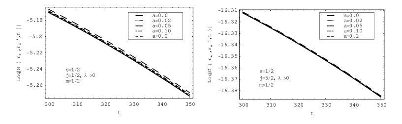
Figure 3: Graphs of ln$|{G^{C}}({r_{\star},{r^{\prime}_{\star}};t})|$ versus $t$ for $j=1/2$ and $j=5/2$, with $Q=0.8$, $\mu=0.01$. The rotating parameter $a$ speeds the decay up for $m\lambda<0$ but slows it down for $m\lambda>0$.

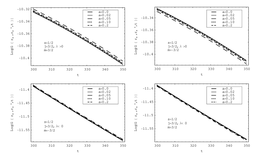
Figure 4: Graphs of ln$|{G^{C}}({r_{\star},{r^{\prime}_{\star}};t})|$ versus $t$, with $Q=-0.8$, $\mu=0.01$, $j=3/2$. The rotating parameter $a$ speeds the decay up for $m\lambda<0$ but slows it down for $m\lambda>0$.

To compare with the oscillating late-time behavior of the massive scalar field in the Kerr-Newman background scalar , we draw the graphs of ln$|{G^{C}}({r_{\star},{r^{\prime}_{\star}};t})|$ versus $t$ with $\mu=0.01$, $Q=0.8$, $a=0.02$ in Fig 5. It is shown that the intermediate late-time behavior of charged massive Dirac field is dominated by a decaying tail without any oscillation, and the decay of the massive Dirac field which is affected by the black-hole and field parameters is slower than that of the massive scalar field.

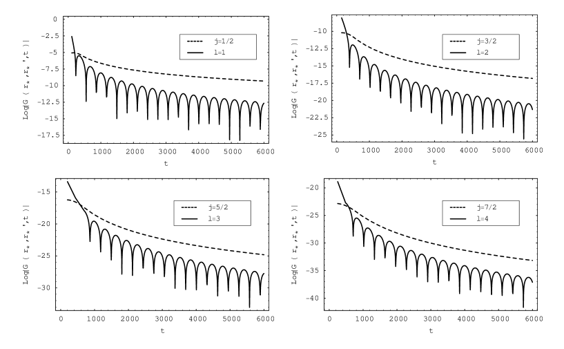
Figure 5: Graphs of ln$|{G^{C}}({r_{\star},{r^{\prime}_{\star}};t})|$ versus $t$ with $\mu=0.01$, $Q=0.8$, $a=0.02$. The dashed lines represent the result of the Green function of the massive Dirac field with different $j$. For comparing, we also show the corresponding result of the scalar field with real lines. It is shown that the late-time behavior of massive Dirac fields is dominated by a decaying tail without any oscillation, and the decay of the massive Dirac field is slower than that of the massive scalar field.

III.2 Asymptotically late-time tail

The intermediate tail is not a final pattern of the perturbation decay. At very late times, $\mu t\gg{1/(\mu M)^{2}}$, we find

$$k\simeq{{M\mu^{2}-eQ\mu\over\varpi}}\gg 1,$$ (41)

which means that the $1/r$ term gives the dominant contribution to the decay. That is to say, the backscattering from the asymptotically far regions is important. Using the Eq. (13.5.13) of Ref. hy , we obtain

$$F(\omega)\simeq{\Gamma(1+2b)\Gamma(1-2b)r_{\star}r^{\prime}_{\star}\over 2b}\left[J_{2b}(\sqrt{\alpha r^{\prime}_{\star}})J_{-2b}(\sqrt{\alpha r_{\star}})-I_{-2b}(\sqrt{\alpha r_{\star}})I_{-2b}(\sqrt{\alpha r_{\star}})\right]+$$

$${\Gamma(1+2b)^{2}\Gamma(-2b)\Gamma({1\over 2}+b-a)r_{\star}r^{\prime}_{\star}\over 2b\Gamma(2b)\Gamma({1\over 2}-b-a)}\left[J_{2b}(\sqrt{\alpha r^{\prime}_{\star}})J_{-2b}(\sqrt{\alpha r_{\star}})+I_{-2b}(\sqrt{\alpha r_{\star}})I_{-2b}(\sqrt{\alpha r_{\star}})\right],$$

where $\alpha=8M\mu^{2}-8eQ\mu$, and $I_{\pm 2b}$ are modified Bessel functions.

It is easily to know that the factor $\Gamma(1+2b)\Gamma(1-2b)/2b$ in the first term is not a constant. Therefore, we use numerical method to study late-time behavior of the first term and present the result in Fig. (6). The figure shows, for different value of $a$, that asymptotically late-time tail arising from the first term is still $\sim t^{-1}$ although the factor $\Gamma(1+2b)\Gamma(1-2b)/2b$ is not a constant.

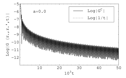
Figure 6: Graphs of ln$|{G^{C}}({r_{\star},{r^{\prime}_{\star}};t})|$ versus $t$ with $M=100$, $\mu=0.01$, $Q=0.1M$, $e=0.002$, $s=-1/2$ and $j=1/2$ (the left panel is for $a=0$ and right one for $a=0.2$) for the first term (solid line). The dashed line is $\sim\log\left|\frac{1}{t}\right|$. From the figure we know, for different $a$, that the late-time tail arising from the first term is $\sim\frac{1}{t}$.

Then we consider the contribution of the second term to the decay rate. Because

$${\Gamma(1+2b)\Gamma(1-2b)\over 2b}=-{\Gamma(1+2b)^{2}\Gamma(-2b)\over 2b\Gamma(2b)},$$ (43)

and the factor almost does not affect the asymptotically behavior of the firs term, we define

$$A={\Gamma(1+2b)^{2}\Gamma(-2b)r_{\star}r^{\prime}_{\star}\over 2b\Gamma(2b)}\left[J_{2b}(\sqrt{\alpha r^{\prime}_{\star}})J_{-2b}(\sqrt{\alpha r_{\star}})+I_{-2b}(\sqrt{\alpha r_{\star}})I_{-2b}(\sqrt{\alpha r_{\star}})\right],$$ (44)

which approximates to a constant. Then, the second term in Eq. (III.2) can be rewritten as

$$G^{C}(r_{\star},r^{\prime}_{\star};t)\simeq{A\over 2\pi}\int_{-\mu}^{\mu}{\Gamma({1\over 2}+b-k)\over\Gamma({1\over 2}-b-k)}a^{-2b}e^{-i\omega t}d\omega.$$ (45)

Using the saddle point integration method, the Eq. (45) can be written as

$$G^{C}(r_{\star},r^{\prime}_{\star};t)\simeq{A\over 2\pi}\int_{-\mu}^{\mu}e^{i(2\pi k-\omega t)}e^{i\phi}d\omega,$$ (46)

where the phase is defined by

$$e^{i\phi}={{1+(-1)^{2b}e^{-2i\pi k}}\over{1+(-1)^{2b}e^{2i\pi k}}},$$ (47)

and it remains in the range $0\leq\phi\leq 2\pi$, even if $k$ becomes very large.

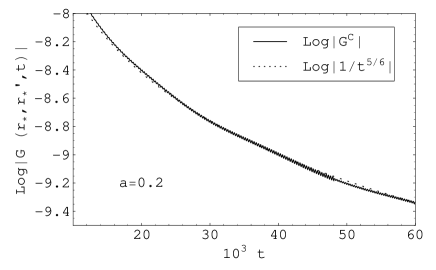
Figure 7: Graphs of ln$|{G^{C}}({r_{\star},{r^{\prime}_{\star}};t})|$ versus $t$ with $M=100$, $\mu=0.01$, $Q=0.1M$, $e=0.002$, $s=-1/2$ and $j=1/2$ (the left panel is for $a=0$ and right one for $a=0.2$) for the second term (solid line). The dashed line is $\sim\log\left|\frac{1}{t^{5/6}}\right|$. The figure shows, for different $a$, that the late-time tail arising from the second term is $\sim\frac{1}{t^{5/6}}$.

Solving

$${d\over d\omega}\ \ (2\pi k-\omega t)\ =\ 0,$$ (48)

we get

$$\varpi_{0}\simeq\left[2\pi(M\mu^{3}-eQ\mu^{2})\over t\right]^{1/3},$$ (49)

at very large times (when $\mu t\gg{1/(\mu M)^{2}}$ is satisfied). In this region, most of the waves backscattered by the space curvature are cancelled by each other, except for the particular waves with the frequency $\omega_{0}\simeq\mu$. Approximating the integral (46) in the immediate vicinity of $\omega_{0}$, we find

$$G^{C}(r_{\star},r^{\prime}_{\star};t) \sim {A\mu\over 2\sqrt{3}}(2\pi)^{5/6}(M\mu-eQ)^{1/3}(\mu t)^{-5/6}$$ (50)

$$\times sin\left\{\mu t-[2\pi(M\mu-eQ)]^{2/3}(\mu t)^{1/3}-\phi(\omega_{0})-{\pi\over 4}\right\}.$$

The equation shows that the decay rate of the asymptotic late-time tail is exactly $t^{-5/6}$, and the oscillation has the period $2\pi/\mu$ which is modulated by two types of long-term phase shift, the one is $[2\pi(M\mu-eQ)]^{2/3}(\mu t)^{1/3}$ represents a monotonously increasing phase shift, the other is $\phi(\omega_{0})$ represents a periodic phase shift.

In order to check the above analytical calculation, we also present the numerical result of the second term in the Fig. 7 and find that the decay rate of the asymptotically tail is $\sim t^{-5/6}$ for different value of $a$.

IV Discussion and Summary

The Teukolsky’s master equations for the charged massive Dirac fields in the Kerr-Newman spacetime are obtained by means of the Newman-Penrose formulism. Then, both the intermediate late-time tail and the asymptotic tail behavior of the charged massive Dirac fields in the background of the Kerr-Newman black hole are studied by considering the intermediate and very late-time solutions of the Teukolsky’s master equations. The results of the intermediate late-time tail are presented by figures because we can not obtain analytically Green’s function $G^{C}(r_{*},r_{*}^{\prime};t)$, as the parameter $b$ in the integrand of the Green’s function depends on the integral variable $\omega$, especially for a factor $\lambda\omega/\mu$. We learn from the figures that the intermediate late-time behavior of charged massive Dirac field is dominated by a decaying tail without any oscillation which is different from the oscillatory decaying tails of the scalar field, and the decay of the massive Dirac field is slower than that of the massive scalar field. We find that the dumping exponent depends not only on the multiple number of the wave mode but also on the product $seQ$ of the spin weight of the Dirac field and the charges of the black hole and the fields ($seQ<0$ speeds up the decay of the charged massive Dirac fields but $seQ>0$ slows it down). We also find, for both positive and negative electric charge of the black hole, that the rotating parameter $a$ slows the decay rate down for $m\lambda>0$ but speeds it up for $m\lambda<0$. And at very late time, the backscattering off the curvature from the asymptotically far regions is dominant. We find, for different value of the angular momentum per unit mass, that the decay rate of the asymptotically late-time tail is $t^{-5/6}$ through both numerical integral method and saddle-point integration method, and the oscillation of the tail has the period of $2\pi/\mu$ which is modulated by two types of long-term phase shifts. Our result seems to suggest that the oscillatory $t^{-5/6}$ tail caused by resonance back scattering at asymptotic late time may be a quit general feature for the late-time decay of the charged massive Dirac fields in stationary black-hole backgrounds.

Appendix A The separation constant

The angular equation (II) can be expressed as

$$\left\{{d^{2}\over d\theta^{2}}+cot\theta{d\over d\theta}+{1\over y}\left[{d^{2}y\over d\theta^{2}}+cot\theta{dy\over d\theta}+{a\mu sin\theta\over-2s\lambda+\mu acos\theta}{dy\over d\theta}\right]+\Theta_{s}+\lambda^{2}\right\}{{}_{s}\zeta_{jm}}=0,$$ (51)

where

$$S_{s} = y{{}_{s}\zeta_{jm}},$$

$$y = \sqrt{2s\lambda-a\mu cos\theta},$$

$$\Theta_{s} = {\mu asin\theta\over{\lambda-2s\mu acos\theta}}H-2s{\partial H\over{\partial\theta}}-{1\over 2{sin^{2}\theta}}+{\mu acos\theta\over{2(-2s\lambda+a\mu cos\theta)}}$$ (52)

$$-H^{2}+{1\over 4}{cot^{2}\theta}-\mu^{2}a^{2}cos^{2}\theta.$$

For the slow rotating black hole, ${{}_{s}\zeta_{jm}}$ and $\lambda^{2}$ can be expanded as

$${{}_{s}\zeta_{jm}} = {}_{s}P_{jm}+{{}_{s}S_{jm}^{(1)}}a+{{}_{s}S_{jm}^{(2)}}a^{2}+O(a^{3}),$$

$$\lambda^{2} = \lambda_{0}^{2}+\lambda_{1}^{2}a+\lambda_{2}^{2}a^{2}+O(a^{3}),$$ (53)

where ${}_{s}P_{jm}$ are the spherical harmonics with $s=\pm 1/2$. The functions ${}_{s}P_{jm}$ and ${}_{s}\zeta_{jm}$ satisfy the orthogonality relations

$$\int{{}_{s}P_{j^{\prime}m^{\prime}}}{{}_{s}P_{jm}}d\Omega=\int{{}_{s}\zeta_{j^{\prime}m^{\prime}}}{{}_{s}\zeta_{jm}}d\Omega=\delta_{j^{\prime}j}\delta_{m^{\prime}m}.$$ (54)

Using the ordinary perturbation theory, we have

$$[D_{0}+\lambda_{0}^{2}]{{}_{s}P_{jm}}=0,$$ (55)

$$[D_{0}+\lambda_{0}^{2}]{{}_{s}S_{jm}^{(1)}}+[D_{1}+\lambda_{1}^{2}]{{}_{s}P_{jm}}=0,$$ (56)

$$[D_{0}+\lambda_{0}^{2}]{{}_{s}S_{jm}^{(2)}}+[D_{1}+\lambda_{1}^{2}]{{}_{s}S_{jm}^{(1)}}+[D_{2}+\lambda_{2}^{2}]{{}_{s}P_{jm}}=0,$$ (57)

with

$$D_{0} = {d^{2}\over{d\theta^{2}}}+cot\theta{d\over{d\theta}}-{2mscos\theta\over{sin^{2}\theta}}-{1\over 2sin^{2}\theta}-{m^{2}\over sin^{2}\theta}+{1\over 4}cot^{2}\theta,$$

$$D_{1} = \left({\mu cos\theta\over 4s\lambda_{0}}-{\mu m\over\lambda_{0}}+2m\omega-2s\omega cos\theta\right),$$

$$D_{2} = \left({m\mu\lambda_{1}^{2}\over 2\lambda_{0}^{3}}-{3\mu^{2}\over 16s^{2}\lambda_{0}^{2}}+{\mu\omega\over\lambda_{0}}-\omega^{2}\right)-\mu\left({\lambda_{1}^{2}\over 8s\lambda_{0}^{3}}+{2sm\mu\over\lambda_{0}^{2}}\right)cos\theta$$ (58)

$$+\left({5\mu^{2}\over 16s^{2}\lambda_{0}}-{\mu\omega\over\lambda_{0}}+\omega^{2}-\mu^{2}\right)cos^{2}\theta.$$

From the lowest order equation (55), we have

$$\lambda_{0}^{2}=(j+{1\over 2})^{2}.$$ (59)

Multiplying equation (56) by ${}_{s}P_{jm}$ from the left side and integrating it over $\theta$, we obtain

$$\lambda_{1}^{2}=-2m\omega+{\mu m\over\lambda_{0}}+\left({\mu\over 4s\lambda_{0}}-2s\omega\right){ms\over j(j+1)}.$$ (60)

Setting

$${}_{s}S_{jm}^{(1)}=\sum_{j^{\prime}}c_{jm}^{j^{\prime}}{{}_{s}P_{j^{\prime}m}},$$ (61)

inserting this into equation (56), then multiplying it by ${}_{s}P_{j^{\prime}m}$ from the left side and integrating it over $\theta$, we have

$$c_{jm}^{j^{\prime}}={A\over{j^{\prime}(j^{\prime}+1)-j(j+1)}}\int{{}_{s}P_{j^{\prime}m}}cos\theta{{}_{s}P_{jm}}d\Omega,$$ (62)

where $A={\mu\over 2s(2j+1)}-2s\omega$. It is non-zero only for $j^{\prime}=j\pm 1$, so we obtain

$$c_{jm}^{j+1} = {A\over 2(j+1)^{2}}{\sqrt{(j+m+1)(j-m+1)(j+s+1)(j-s+1)\over(2j+1)(2j+3)}},$$

$$c_{jm}^{j-1} = -{A\over 2j^{2}}{\sqrt{(j+m)(j-m)(j+s)(j-s)\over(2j-1)(2j+1)}}.$$ (63)

In order to obtain $\lambda_{2}^{2}$, we multiply equation (57) by ${}_{s}P_{jm}$ from the left side, and integrate it over $\theta$, then we get

$$\lambda_{2}^{2}= -\int{{}_{s}P_{jm}}D_{1}{{}_{s}S_{jm}^{(1)}}d\Omega-\int{{}_{s}P_{jm}}D_{2}{{}_{s}P_{jm}}d\Omega$$ (64)

$$= -2(j+1)\left(c_{jm}^{j+1}\right)^{2}+2j\left(c_{jm}^{j-1}\right)^{2}$$ (65)

$$-\left({m\mu\lambda_{1}^{2}\over 2\lambda_{0}^{3}}-{3\mu^{2}\over 16s^{2}\lambda_{0}^{2}}+{\mu\omega\over\lambda_{0}}-\omega^{2}\right)-\left({\lambda_{1}^{2}\over 8s\lambda_{0}^{3}}+{2sm\mu\over\lambda_{0}^{2}}\right){\mu ms\over j(j+1)}$$

$$-\left({5\mu^{2}\over 16s^{2}\lambda_{0}}-{\mu\omega\over\lambda_{0}}+\omega^{2}-\mu^{2}\right)\left[{1\over 3}+{2\over 3}{[3m^{2}-j(j+1)][3s^{2}-j(j+1)]\over j(j+1)(2j+3)(2j-1)}\right].$$

The integrals in the above equations are given by

$$\int{{}_{s}P_{j^{\prime}m}}cos\theta{{}_{s}P_{jm}}d\Omega = \sqrt{2j+1\over 2j^{\prime}+1}<j,m,1,0|j^{\prime},m><j,-s,1,0|j^{\prime},-s>,$$

$$\int{{}_{s}P_{j^{\prime}m}}sin^{2}\theta{{}_{s}P_{jm}}d\Omega = {2\over 3}{\delta_{j^{\prime}j}}-{2\over 3}{\sqrt{2j+1\over 2j^{\prime}+1}}<j,m,2,0|j^{\prime},m><j,-s,2,0|j^{\prime},-s>.$$

References

- (1) V. P. Frolov, and I. D. Novikov, Black hole physics: basic concepts and new developments (Kluwer Academic, Dordrecht, 1998).
- (2) R. H. Price, Phys. Rev. D 5 (1972) 2419; R. H. Price and L. M. Burko, Phys. Rev. D 70 (2004) 084039.
- (3) R. H. Price , Phys. Rev. D 5 (1972) 2439.
- (4) E. Poisson and W. Israel, Phys. Rev. D 41 (1990) 1796.
- (5) L. M. Burko, Phys. Rev. Lett 79 (1997) 4958.
- (6) R. Ruffini and J. A. Wheeler, Phys. Today 24(1) (1971) 30.
- (7) C. W. Misner, K. S. Thorne, and J. A. Wheeler, Gravitation (Freeman, San Francisco, 1973).
- (8) N. Andersson, Phys. Rev. D. 55 (1997) 468.
- (9) L. M. Burko and A. Ori, Phys. Rev. D. 56(1997) 7820.
- (10) S. Hod and T. Piran, Phys. Rev.D 58 (1998) 024017.
- (11) S. Hod and T. Piran, Phys. Rev.D 58 (1998) 024018.
- (12) S. Hod and T. Piran, Phys. Rev.D 58 (1998) 024019.
- (13) L. Barack, Phys. Rev.D 59 (1999) 044017.
- (14) J. L. Jing, Phys. Rev. D. 72 (2005) 027501.
- (15) L. Barack and A. Ori, Phys. Rev. Lett. 82 (1999) 4388.
- (16) L. M. Burko and G. Khanna , Phys. Rev. D. 67 (2003) 081502(R).
- (17) A. A. Starobinskii and I. D. Novikov (unpublished).
- (18) L. M. Burko, Abstracts of Plenary Talks and Contributed Papers, 15th International Conference on General Relativity and Gravitation, Pune, 1997, p. 143 (unpublished).
- (19) S. Hod and T. Piran, Phys. Rev.D 58 (1998) 044018.
- (20) L.H. Xue, B. Wang, and R. K. Su, Phys. Rev. D. 66 (2002) 024032.
- (21) H. Koyama and A. Tomimatsu, Phys. Rev. D. 63 (2001) 064032.
- (22) H. Koyama and A. Tomimatsu, Phys. Rev. D. 64 (2001) 044014.
- (23) L. M. Burko and G. Khanna , Phys. Rev. D. 70 (2004) 044018.
- (24) J. L. Jing, Phys. Rev. D. 70(2004) 065004.
- (25) R. Moderski and M. Rogatko, Phys. Rev. D. 64 (2001) 044024.
- (26) R. Moderski and M. Rogatko, Phys. Rev. D. 72 (2005) 044027.
- (27) R. A. Konoplya and C.Molina, gr-qc 0602047 (2006) .
- (28) S. Hod and T. Piran, Phys. Rev. D. 58 (1998) 024017 .
- (29) E. S. C. Ching, P. T. Leung, W. M. Suen, and K. Young , Phys. Rev. D. 52 (1995) 2118.
- (30) E. W. Leaver, Phys. Rev. D. 34 (1986) 384.
- (31) S. Hod and T. Piran, Phys. Rev. D. 58 (1998) 024019.
- (32) D. N. Page, Phys. Rev. D. 14 (1976) 1509.
- (33) E. Newman and R. Penrose, J. Math. Phys. (N.Y) (1962) 3566.
- (34) P. M. Morse and H. Feshbach, Methods of Theoretical Physics (McGraw-Hill, New York, 1953).
- (35) M. Abramowitz and I. A. Stegun, Handbook of Mathematical Functions (Dover, New York, 1970).
- (36) Q. Y. Pan and J. L. Jing, Chin. Phys. Lett. 21 (2004) 1873.