Inspiral, merger and ring-down of equal-mass black-hole binaries

Abstract

We investigate the dynamics and gravitational-wave (GW) emission in the binary merger of equal-mass black holes as obtained from numerical relativity simulations. The simulations were performed with an evolution code based on generalized harmonic coordinates developed by Pretorius, and used quasi-equilibrium initial data sets constructed by Cook and Pfeiffer. Results from the evolution of three sets of initial data are explored in detail, corresponding to different initial separations of the black holes, and exhibit between $2\mbox{--}8$ GW cycles before coalescence. We find that to a good approximation the inspiral phase of the evolution is quasi-circular, followed by a “blurred, quasi-circular plunge” lasting for about $1\mbox{--}1.5$ GW cycles. After this plunge the GW frequency decouples from the orbital frequency, and we define this time to be the start of the merger phase. Roughly $10\mbox{--}15m$ separates the time between the beginning of the merger phase and when we are able to extract quasi-normal ring-down modes from gravitational waves emitted by the newly formed black hole. This suggests that the merger lasts for a correspondingly short amount of time, approximately $0.5\mbox{--}0.75$ of a full GW cycle. We present first-order comparisons between analytical models of the various stages of the merger and the numerical results—more detailed and accurate comparisons will need to await numerical simulations with higher accuracy, better control of systemic errors (including coordinate artifacts), and initial configurations where the binaries are further separated. During the inspiral, we find that if the orbital phase is well modeled, the leading order Newtonian quadrupole formula is able to match both the amplitude and phase of the numerical GW quite accurately until close to the point of merger. We provide comparisons between the numerical results and analytical predictions based on the adiabatic post-Newtonian (PN) and non-adiabatic resummed-PN models (effective-one-body and Padé models). For all models considered, 3PN and 3.5PN orders match the inspiral numerical data the best. From the ring-down portion of the GW we extract the fundamental quasi-normal mode and several of the overtones. Finally, we estimate the optimal signal-to-noise ratio for typical binaries detectable by GW experiments. We find that when the merger and ring-down phases are included, binaries with total mass larger than $40M_{\odot}$ (sources for ground-based detectors) are brought in band and can be detected with signal-to-noise up to $\approx 15$ at 100 Mpc, whereas for binaries with total mass larger than $2\times 10^{6}M_{\odot}$ (sources for space-based detectors) the SNR can be $\approx 10^{4}$ at 1Gpc.

I Introduction

With gravitational-wave (GW) detectors operating LIGO ; GEO ; TAMA or under commissioning VIRGO , it is more and more desirable to improve the theoretical predictions of the GW signals. Compact binaries composed of black holes (BH) and/or neutron stars are among the most promising candidates for the first detection.

The last year has been marked by breakthroughs in numerical relativity (NR) with several independent groups being able to simulate binary black hole coalescence through the last stages of inspiral ($2\mbox{--}4$ orbits), merger, ring-down and sufficiently long afterwards to extract the emitted GW signal FP ; Bakeretal1 ; CLMZ ; HLS ; S . In Ref. FP the first stable evolution of such an entire merger process was presented. A couple of the key elements responsible for this success where the use of a formulation of the field equations based on a generalization of harmonic coordinates friedrich ; garfinkle ; szilagyi_et_al and the addition of constraint damping terms to the equations gundlach_et_al ; lambda_ref . Similar techniques have been successfully incorporated into other efforts since lindblom_et_al ; scheel_et_al ; szilagyi_nfnr . Some months afterwords, two groups CLMZ ; Bakeretal1 independently presented modifications of the BSSN (or NOK) nok ; bs ; sn formulation of the field equations that allowed them to simulate complete merger events. Among the key modifications were gauge conditions allowing the BHs to move through the computational domain in a so-called puncture evolution bruegmann ; these methods have also been successfully reproduced by other groups since HLS ; S ; bruegmann_nfnr ; marronetti_nfnr ; pollney_nfnr .

In this paper, after analyzing the main features of the dynamics and waveforms obtained from the NR simulations, we present a preliminary comparison between the numerical and analytical waveforms. The analytical model we use for the inspiral phase is the post-Newtonian (PN) approximation 35PNnospin ; LB in the adiabatic limit  LB , whereas for the inspiral–(plunge)–merger–ring-down phases we consider the PN non-adiabatic and resummed models, such as the effective-one-body (EOB) BD1 ; BD2 ; BD3 ; DJS ; TD ; BCD and Padé resummations DIS98 . Due to the limited resolution, initial eccentricity, relatively close initial configurations and possible coordinate artifacts, it is difficult to claim very high accuracy when comparing with analytical models. Thus, we shall refer to those comparisons as first-order comparisons. We will only consider a few dynamical quantities of the analytical models characterizing the binary evolution, notably gauge-invariant quantities such as the orbital and wave frequencies, and the GW phase, all as measured by an observer at infinity. When comparing, we will assume that the numerical and analytical waveforms refer to equal-mass binaries, but we apply a fitting procedure to obtain the best-match time of coalescence and the spin variables. We will use the confrontation with analytical models as an interesting diagnostic of the numerical results. When simulations that are more accurate and begin closer to an inspiralling circular binary become available we will be able to do more stringent tests of analytical models, compare all dynamical quantities expressed in the same gauge, and use those results to discriminate between models.

Certainly, the most intriguing and long-awaited result of the numerical simulation is the transition inspiral–merger–ring-down. Is it a strongly non-linear phase? How much energy and angular momentum is released? Over how many GW cycles does it occur? How spread in frequency is the signal power spectrum? Answers to these questions are relevant from a theoretical point of view, e.g., to study general relativity in the strongly coupled regime, and also from an observational point of view, e.g., to build faithful templates to detect GW waves and test GR with GW experiments. In this paper we shall start to scratch the surface of this problem. We pinpoint several interesting features of the inspiral to ringdown transition that need to be investigated more quantitatively in the future when more accurate simulations become available.

Quasi-normal modes (QNM) (or ring-down modes) of Schwarzschild and Kerr BHs were predicted a long time ago CVV ; Press ; Davis ; QNR . Their associated signal can be described analytically in terms of damped sinusoids. By fitting to the numerical waveforms we extract the dominant QNMs of the final Kerr BH—i.e. the fundamental mode and several of the overtones—and try to make connections to the previous dynamical phase.

Finally, we discuss the impact of the merger and ring-down phases on the detectability of GWs emitted by equal-mass binaries for ground-based and space-based detectors, and compare those results with predictions from analytical models.

This paper is organized as follows. In Sec. II we review the initial-data sets of Cook and Pfeiffer CP used in the numerical simulations. In Sec. III we present and discuss the results of NR simulations of binary BH mergers obtained with the generalized-harmonic-gauge code of Pretorius FP . In Sec. IV we provide a first-order comparison between numerical and analytical results for the last stages of inspiral. In Secs. V and VI we analyze the ring-down and merger phases as predicted by the numerical simulations. In Sec. VII we present a first-order comparison between the numerical results and the EOB predictions for inspiral, plunge, merger and ring-down. In Sec. VIII we evaluate the Fourier transform of the waveforms and discuss how the inclusion of the merger and ring-down phases will increase the optimal signal-to-noise ratio of ground-based and space-based detectors. Section IX contains our main conclusions and a discussion on how to make more robust comparisons with analytical models in future NR simulations.

Some material we defer to appendices. The majority of the comparisons and analysis of gravitational waveforms focus on the dominant quadrupole multipole moment of the wave; in Appendix A we briefly describe the sub-dominant multipole moments extracted from the waves. Appendix B compares the energy and angular momentum flux of the numerically extracted GW with analytical models of the fluxes. In Appendix C we describe some possible artifacts induced by extracting the GW a finite distance from the source in the simulations. Appendix D contains tables of fitting coefficients from the QNM ring-down fits. We have analyzed three sets of BBH evolutions—some figures from the case with the closest initial separation are contained in Appendix E to simplify the main text.

II Initial data

The evolutions presented in this paper begin with initial data that has been prepared using the methods developed by Cook and Pfeiffer CP ; CCGP ; PKST ; CPID . This approach incorporates the extended conformal thin-sandwich (CTS) decomposition PY ; CTS , the “Komar mass method” for locating circular orbits GGB1 ; GGB2 , and quasiequilibrium boundary conditions on BH excision surfaces C2 ; CP . The data we have used are designed to represent an equal-mass binary BH configuration in which the binary is in quasiequilibrium with the holes in a nearly circular orbit and where the spins of the individual holes correspond to “corotation”. Within the CTS approach, the conformal metric, the trace of the extrinsic curvature, and their time derivatives must be freely specified. The time derivatives of the conformal metric and the trace of the extrinsic curvature are chosen to vanish. This time derivative is taken along an approximate helical Killing vector which defines the notion of quasiequilibrium. The initial data is constructed on a “maximal slice” which fixes the trace of the extrinsic curvature to zero. Finally, the conformal metric is chosen to be flat.

The initial data produced by this procedure do a very good job of representing the desired astrophysical situation of a pair of BHs nearing the point of coalescence. However, two important approximations have been made in the construction of these initial-data sets. When the initial data are evolved, these approximations will affect the subsequent dynamics and the GW that is produced. The first approximation is that the initial data are “conformally flat”. The choice of a flat conformal metric is known to introduce small errors in representing both individual spinning BHs and binary systems. As part of this error, some amount of unphysical gravitational radiation is included in the initial data. The second approximation is in placing the binary in a circular orbit. This approximation is motivated by the fact that for large enough separation, the time scale for radial motion due to radiation reaction is large compared to the orbital period. However, this approximation results in BHs having little, if any, initial radial momentum. For sufficiently small separations, this is clearly not “astrophysically correct.”

Until now, the best way to estimate the quality of BH binary initial data has been to compare them against the results obtained by PN methods. Comparisons of gauge-invariant quantities such as the total energy and angular momentum of the system or the orbital angular velocity, all measured at infinity, are in good agreement with adiabatic sequences of circular orbits as determined by third-order PN (3PN) calculations LB and their EOB resummed extension BD1 ; DJS (see Figs. 10–18 in Ref. CP , Figs. 3–5 in Ref. DGG and Figs. 3–5 in Ref. ICO and discussion around them). There are, of course, differences between the numerical initial data and the PN/EOB models and these differences increase as the binary separation decreases and the system becomes more relativistic. Among these differences, there is also some evidence that the initial orbit incorporates a small eccentricity BIW .

Adiabatic sequences of BH binaries exhibit an inner-most stable circular orbit (ISCO) defined by a turning point in the total conserved energy. For the numerical initial data, the quasiequilibrium approximation becomes less accurate as the binary separation decreases and we would expect the approximation to be rather poor at the ISCO. PN methods restricted to circular orbits suffer similar problems as they approach the ISCO. The PN/EOB and numerical initial-data circular-orbit models are in reasonable agreement up to the ISCO, but it is difficult to ascertain the accuracy of either in this limit.

The comparisons done in Refs. DGG ; ICO ; CP between numerical initial data and PN/EOB models are limited by the fact that they use adiabatic circular orbits. Essentially, these comparisons lend strength to the belief that the conformal-flatness approximation is not causing significant problems with the non-radiative aspects of the initial data. Clearly, they cannot shed any light on the effects of the circular-orbit approximation. Some insight on this issue has been obtained by performing full dynamical evolutions of the PN/EOB equations of motion for equal-mass binaries BD2 ; MM . These studies show that neglecting the radial momentum, at both the initial time and throughout the evolution as done in adiabatic circular orbits, results in a phase error in the waveforms (see e.g., Fig. 5 in Ref. BD2 ). Neglecting the radial momentum at the initial time also introduces eccentricity into the dynamics (see e.g., Fig. 4 in Ref. MM ).

III Numerical relativity results and their diagnostics

III.1 Initial Data for Generalized Harmonic Evolution

The corotating quasi-circular BH inspiral data discussed in the previous section were evolved using a numerical code based on a generalized harmonic (GH) decomposition of the field equations, as described in detail in Ref. FP1 ; FP ; FP3 . As supplied by Pfeiffer CPID ; PKST , the initial data is given in terms of standard $3+1$ or ADM (Arnowitt-Deser-Misner) variables L ; ADM ; CB ; Y , namely the lapse function $\alpha$, shift vector $\beta^{i}$, spatial metric $h_{ij}$ and extrinsic curvature $K_{ij}$:

$$ds^{2} = -\alpha^{2}dt^{2}+h_{ij}\left(dx^{i}+\beta^{i}dt\right)\left(dx^{j}+\beta^{j}dt\right),$$ (1)

$$K_{ij} = -h_{i}{}^{l}h_{j}{}^{m}\nabla_{m}n_{l}.$$ (2)

In the above $n_{\mu}=-\alpha\nabla_{\mu}t$ is the unit time-like vector normal to $t={\rm const.}$ hypersurfaces, and we use units where $G=c=1$. The GH code directly integrates the 4-metric elements $g_{\mu\nu}$

$$ds^{2}=g_{\mu\nu}dx^{\mu}dx^{\nu},$$ (3)

and therefore needs the values of $g_{\mu\nu}$ and $\partial g_{\mu\nu}/\partial t$ at $t=0$ as initial conditions. The initial data (1), (2) provides most of what is required to construct $g_{\mu\nu}|_{t=0},\partial g_{\mu\nu}/\partial t|_{t=0}$; what must still be specified are the components of the gauge encoded in $\partial\alpha/\partial t|_{t=0}$ and $\partial\beta^{i}/\partial t|_{t=0}$. We choose the time derivatives of the lapse and shift such that the slice is spacetime harmonic at $t=0$:

$$\partial_{\gamma}\alpha\ n^{\gamma} = -\alpha K$$ (4)

$$\partial_{\gamma}\beta^{i}\ n^{\gamma} = \alpha\bar{\Gamma}^{i}_{jk}h^{jk}-\partial_{j}\alpha\ h^{ij},$$ (5)

where $K$ is the trace of the extrinsic curvature, and $\bar{\Gamma}^{i}_{jk}$ are the Christoffel symbols of the spatial metric $h_{ij}$.

III.2 Characterization of the Waveform

Gravitational wave information is obtained by computing the Weyl scalar $\Psi_{4}$, which has the asymptotic property of being equal to the outgoing radiation if the complex null tetrad is chosen correctly. To be explicit, we define a spherical coordinate system centered on the center of mass of the binary with orthonormal bases $(\hat{r},\hat{\theta},\hat{\phi})$. The coordinates are chosen so that the azimuthal axis is aligned with the orbital angular momentum and the binary orbits in the direction of increasing azimuthal coordinate.

To define our complex null tetrad, we use the time-like unit vector normal to a given hypersurface $\hat{n}$ and the radial unit vector $\hat{r}$ to define an ingoing ($\vec{k}$) and outgoing null vector ($\vec{\ell}$) by

$$\vec{k} \equiv \frac{1}{\sqrt{2}}(\hat{n}+\hat{r}),$$ (6)

$$\vec{\ell} \equiv \frac{1}{\sqrt{2}}(\hat{n}-\hat{r}).$$ (7)

We define the complex null vector $\vec{m}$ by

$$\vec{m}\equiv\frac{1}{\sqrt{2}}(\hat{\phi}-i\hat{\theta}).$$ (8)

In terms of this tetrad, we define $\Psi_{4}$ as

$$\Psi_{4}\equiv C_{\alpha\beta\gamma\delta}\ell^{\alpha}(m^{\beta})^{*}\ell^{\gamma}(m^{\delta})^{*},$$ (9)

where $C_{\alpha\beta\gamma\delta}$ is the Weyl tensor and $*$ denotes complex conjugation.

To relate $\Psi_{4}$ to the GWs, we note that in transverse-traceless (TT) gauge,

$$\frac{1}{4}(\ddot{h}^{TT}_{\hat{\theta}\hat{\theta}}-\ddot{h}^{TT}_{\hat{\phi}\hat{\phi}}) = -R_{\hat{n}\hat{\theta}\hat{n}\hat{\theta}}=-R_{\hat{n}\hat{\phi}\hat{r}\hat{\phi}}=-R_{\hat{r}\hat{\theta}\hat{r}\hat{\theta}}=R_{\hat{n}\hat{\phi}\hat{n}\hat{\phi}}=R_{\hat{n}\hat{\theta}\hat{r}\hat{\theta}}=R_{\hat{r}\hat{\phi}\hat{r}\hat{\phi}},$$ (10)

$$\frac{1}{2}\ddot{h}^{TT}_{\hat{\theta}\hat{\phi}} = -R_{\hat{n}\hat{\theta}\hat{n}\hat{\phi}}=-R_{\hat{r}\hat{\theta}\hat{r}\hat{\phi}}=R_{\hat{n}\hat{\theta}\hat{r}\hat{\phi}}=R_{\hat{r}\hat{\theta}\hat{t}\hat{\phi}}.$$ (11)

Following convention, we take the $h_{+}$ and $h_{\times}$ polarizations of the GW to be given by

$$\ddot{h}_{+} = \frac{1}{2}(\ddot{h}^{TT}_{\hat{\theta}\hat{\theta}}-\ddot{h}^{TT}_{\hat{\phi}\hat{\phi}}),$$ (12)

$$\ddot{h}_{\times} = \ddot{h}^{TT}_{\hat{\theta}\hat{\phi}}.$$ (13)

We find, then, that in vacuum regions of the spacetime,

$$\Psi_{4}=\ddot{h}_{+}-i\ddot{h}_{\times}.$$ (14)

It is most convenient to deal with $\Psi_{4}$ in terms of its harmonic decomposition. Given the definition of $\Psi_{4}$ in Eq. (9) and the fact that $\vec{m}^{*}$ carries a spin-weight of $-1$, it is appropriate to decompose $\Psi_{4}$ in terms of spin-weight $-2$ spherical harmonics ${}_{-2}Y_{\ell m}(\theta,\phi)$. There is some freedom in the definition of the spin-weighted spherical harmonics. To be explicit, we defined the general spin-weighted spherical harmonics by

$${}_{s}Y_{\ell m}(\theta,\phi)\equiv(-1)^{s}\sqrt{\frac{2\ell+1}{4\pi}}d^{\ell}_{m(-s)}(\theta)e^{im\phi},$$ (15)

where $d^{\ell}_{ms}$ is the Wigner $d$-function

$$d^{\ell}_{ms}(\theta)\equiv\sum_{t=C_{1}}^{C_{2}}\frac{(-1)^{t}\sqrt{(\ell+m)!(\ell-m)!(\ell+s)!(\ell-s)!}}{(\ell+m-t)!(\ell-s-t)!t!(t+s-m)!}(\cos\theta/2)^{2\ell+m-s-2t}(\sin\theta/2)^{2t+s-m},$$ (16)

and where $C_{1}=\max(0,m-s)$ and $C_{2}=\min(\ell+m,\ell-s)$.

Finally, for convenience, we always decompose the dimensionless Weyl scalar $rM\Psi_{4}$ where $M=m_{1}+m_{2}$ is the mass of the initial binary system with $m_{1}$ and $m_{2}$ the irreducible CR masses of the individual BHs, and $r$ is the generalized harmonic radial coordinate. We then define

$$rM\Psi_{4}(t,\vec{r})=\sum_{\ell m}{}_{-\!2}C_{\ell m}(t,r){}_{-\!2}Y_{\ell m}(\theta,\phi).$$ (17)

The complex mode amplitudes ${}_{-\!2}C_{\ell m}(t,r)$, extracted at a fixed generalized harmonic coordinate radius $r$, contain the full information about the gravitational waveforms as a time-series.

In the numerical code the four orthonormal vectors $(\hat{n},\hat{r},\hat{\theta},\hat{\phi})$ used to construct the null tetrad are computed as follows. The spacetime is evolved using Cartesian coordinates $x,y,z$ with time $t$, and we use the standard transformation to define the spherical coordinates:

$$x = r\cos(\phi)\sin(\theta)\,,$$ (18)

$$y = r\sin(\phi)\sin(\theta)\,,$$ (19)

$$z = r\cos(\theta)\,,$$ (20)

$\hat{n}$ is the time-like unit vector normal to $t={\rm const.}$ surfaces, and $\hat{r}$ is the unit space-like vector pointing in the direction $(\partial/\partial r)^{a}$. In the limit $r\rightarrow\infty$ the time coordinate $t$ coincides with $TT$ time. $\hat{\theta}$ is computed by making $(\partial/\partial\theta)^{a}$ orthonormal to $(\hat{n},\hat{r})$ using a Gramm-Schmidt process, and then $\hat{\phi}$ is calculated by making $(\partial/\partial\phi)^{a}$ orthonormal to ($\hat{n},\hat{r},\hat{\theta}$). All norms are computed with the full spacetime metric $g_{\mu\nu}$. The Weyl scalar $\Psi_{4}$ is evaluated over the entire numerical grid (i.e. at all $x,y,z$ mesh points) at regular intervals in time. We then interpolate $\Psi_{4}(t,x,y,z)$ to a set of coordinate spheres at several “extraction radii” $r_{i}$, with a uniform distribution of points in $(\theta,\phi)$ . All the waveform related data from the simulations presented here are taken from such samplings of $\Psi_{4}(t,r=r_{i},\theta,\phi)$, and we have used $r_{i}=12.5m,25m,37.5m$ and $50m$. The plots and comparisons shown in the main part of the paper use $r_{i}=50m$, while in Appendix C we discuss the trends that are seen in $\Psi_{4}$ as a function of $r_{i}$. To summarize the results of the Appendix, prior to merger the extraction radii at $37.5m$ and $50m$ appear to be well within the “wave-zone”, and thus gives a decent representation of the waveform. Specifically, the coordinate propagation speed of the wave from one extraction sphere to the next is very close to unity, and the structure of the wave, normalized by $r$, is similar at the two extraction points. Interestingly though, at later times during the simulation, apparently in coincidence with the strongest wave emission around the merger part of the evolution, the gauge seems to change slightly in the extraction zone. The coordinate speed drops by several percent, and the amplitude of the normalized waveform also decreases as the wave moves outward. The effect is more pronounced for binaries that are initially further separated. As not all metric information was saved when the simulations were run we cannot describe what underlying properties of the metric are responsible for the change in propagation behavior, though for the purposes of this paper the effect is sufficiently small that we do not believe it will alter any of the primary conclusions. A couple of exceptions are in the estimates of the total energy and angular momentum radiated—these calculations involve double and triple time integrations of squares of the wave, and so significantly amplify even small systematic errors in the waveform. This is, we believe, the cause of the increasing over-estimate of these quantities as the initial orbital separation increases, as shown later in Table 2. Future work will attempt to address these gauge-related issues.

III.3 Numerical results and a discussion of errors

We have evolved 3 sets of initial data, labeled by $d=13,16$ and $19$ in Ref. CP ; the initial orbital parameters are summarized in Table 1 . Each initial data set was evolved using three different grid resolutions, summarized in Table 2. Most of the results presented in this paper are from the highest resolution simulations, with the lower resolution runs providing error estimates via the Richardson expansion. During evolution the same temporal source-function evolution equations were used as with the scalar-field-collapse binaries described in Ref. FP1 ; FP , and the (covariant) spatial source-functions were kept equal to zero. We have quite extensively tested this code to make sure we are solving the Einstein equations, and convergence tests of the residual of the Einstein equation for similar simulations were presented in Ref. FP3 .

	“d”	$M_{\rm ADM}/M$	$M\omega$	$J_{\rm ADM}/M^{2}$	$\ell/M$	$S_{1}/m_{1}^{2}$
	13	0.986	0.0562	0.875	7.96	0.107
	16	0.988	0.0416	0.911	9.77	0.0802
	19	0.989	0.0325	0.951	11.5	0.0629

Table 1: Several parameters describing the initial data CP (left to right): the ADM mass of the spacetime, the initial angular velocity of each BH, the ADM angular momentum, the initial proper separation between the holes, and their initial spins. The units have been scaled to $M$, the sum of initial AH masses.

	“Resolution”	wave-zone res.	orbital-zone res.	BH res.
	h	$1.6M$	$0.20M$	$0.048M$
	3/4 h	$1.2M$	$0.15M$	$0.036M$
	1/2 h	$0.82M$	$0.10M$	$0.024M$

Table 2: The three sets of characteristic spatial resolutions used in the simulation discussed here, where each resolution is labeled relative to the coarsest resolution $h$. The grid is adaptive with a total of 8 levels of refinement, and the coordinate system is compactified. The wave zone is defined to be at $r=50M$, the orbital zone within about $r=10M$ and the BH zone is within $2-3M$ of each AH. A Courant-Friedrichs-Lewy (CFL) factor of $0.2$ was used in all cases.

	d=13	d=16	d=19
$M_{f}/M$	$0.950\pm 0.005$	$0.954\pm 0.005$	$0.952\pm 0.005$
$E_{\rm GW}/M$	$0.036\pm 0.004$	$0.043\pm 0.004$	$0.052\pm 0.004$
$a_{f}/M_{f}$	$0.71\pm 0.02$	$0.71\pm 0.02$	$0.70\pm 0.02$
$J^{z}_{f}/M^{2}$	$0.64\pm 0.02$	$0.65\pm 0.02$	$0.63\pm 0.02$
$J^{z}_{\rm GW}/M^{2}$	$0.23\pm 0.02$	$0.31\pm 0.02$	$0.42\pm 0.02$
number of orbits	$1.47\pm 0.10$	$2.47\pm 0.09$	$4.39\pm 0.18$
$t_{\rm CAH}/M$	$109\pm 4$	$228\pm 16$	$529\pm 22$
$(t_{\rm peak}-t_{\rm CAH})/M$	$\approx 9$	$\approx 9$	$\approx 9$
$(t_{\rm dec}-t_{\rm CAH})/M$	$\approx-11$	$\approx-11$	$\approx-9$
initial eccentricity $e_{1}$	—	—	$0.018\pm 0.003$
initial eccentricity $e_{2}$	—	—	$0.012(+0.014,-0.012)$
Max. GW amp. error	8%	9%	8%
(Max. GW phase error)/$(2\pi)$	0.08	0.7	1
(Max.“shifted” GW phase error)/$(2\pi)$	0.04	0.06	0.05

Table 3: A summary of simulation results. From top to bottom: (i) the mass $M_{f}$ of the final BH estimated from AH properties, (ii) the energy $E_{\rm GW}$ emitted in GWs extracted using the Newman-Penrose scalar $\Psi_{4}$ at a coordinate radius of $r=50M$ from the origin, (iii) the Kerr spin parameter $a_{f}$ and corresponding non-zero z-component $J^{z}$ of the angular-momentum vector of the final BH (from AH properties), (iv) an estimate $J^{z}_{\rm GW}$ of the angular-momentum radiated in GWs (from $\Psi_{4}$), (v) the number of orbits in coordinate space before a common AH, at coordinate time $t=t_{\rm CAH}$, is first detected, (vi) an estimate $t=t_{\rm peak}$ of when the GW amplitude reaches its peak, (vii) an estimate $t=t_{\rm dec}$ of when the GW frequency decouples from the orbital frequency, (viii) for $d=19$ two estimates of the eccentricity in the initial data calculated using (21) ($e_{1}$) and (22) ($e_{2}$), (ix) the estimated maximum error in the amplitude of the extracted GWs (occurring near the peak of emission), (x) an estimate of the cumulative phase error in the wave from $t=0$ until merger, and (xi) the phase error after maquillage. The estimated uncertainties and errors do not include possible systematic errors; see the discussion in Secs. III.2, III.3 and Appendix C for more information. In all plots in the paper where we have shifted time by either $t_{\rm CAH}$ or $t_{\rm peak}$, any quantity shown that was measured from the waveform at $r=50M$ is also shifted by the propagation time $\delta t$ of the wave to $r=50M$. We have estimated $\delta t$ by finding the shift resulting in a best-fit between orbital frequency measured using the GW versus AH orbital motion, as shown in Fig. 7; specifically, we get $\delta t=65M,68M$ and $70M$ for $d=13,16$ and $19$ respectively.

Table 3 lists some key information obtained from each merger simulation. Figure 1 shows the orbital motion prior to merger. The uncertainties and error estimates listed in the table were calculated using an assumed Richardson expansion, as discussed in FP3 . At least three simulations are needed to verify that one is in the convergent regime in general, and for the properties listed in the table we do see close to second order convergence for most properties — a couple of anomalous cases (the phase error and merger time for the $d=19$ case) are discussed further below. Assuming one is in the convergent regime, results from two simulations can then be used to estimate the truncation error. This estimate will not account for systematic errors, and here we list several potential sources of such error. Some quantities are in principle susceptible to gauge or coordinate effects, including the apparent horizons (AHs), and therefore properties measured using them; orbital parameters such as angular frequency and eccentricity deduced from the positions of the AHs; the finite GW extraction radius and nature of the coordinates at the extraction surface (see Sec.III.2 and AppendixC); and the choice of tetrad used to calculate $\Psi_{4}$ NBRE ; NBBBP ; BBLP . Certain post-processing operations have a truncation error associated with them and we have not estimated the magnitude of these. For example, in all cases $\Psi_{4}$ was sampled on a mesh of size $33\times 65$ points in $\theta\times\phi$ at the extraction radius at a given time. We suspect that many of these systematic errors are small, though eventually the accuracy of the simulations will be improved (through a combination of high-order methods and higher resolution), and then it may become important to quantify and eliminate these additional uncertainties.

In a waveform, the error of most significance to GW detection is an error in the phase. The first generation of numerical binary BH merger simulations FP ; Bakeretal1 ; CLMZ ; Bakeretal2 ; CLZ ; HLS ; FP3 ; CLZ2 , with the notable exception of the Caltech/Cornell effort CalCor , all suffer from rather significant cumulative phase errors in the inspiral portion of the waveform for the longer duration merger events. In Ref. Bakeretal2 it was argued that the dominant portion of the phase could be factored out as a constant phase shift within the wave, resulting in a “universal” merger result for the class of initial conditions considered. Henceforth, we shall denote by maquillage the operation of phase shifting waveforms to make them agree at a specified point in time, improving their coincidence (appeareance) over a larger interval of time. For certain applications this maquillage waveform is the relevant one. For example, in a matched-filter search the initial phase of the waveform is an extrinsic parameter DIS98 and is irrelevant for detectability of the signal. Also, when comparing waveforms from different initial-data sets the waveforms need to be aligned in some manner for a meaningful comparison, and so again a constant phase difference, whatever the source, is largely irrelevant. However, for parameter estimation in an inspiral search where a hybrid PN/numerical template is used, the association of a numerical merger/ring-down to a PN inspiral waveform will be very sensitive to all phase errors. In particular, an uncertainty in the overall phase evolution prior to merger in the numerical waveform is directly related to an uncertainty in the merger time for the given initial conditions, and this will translate to an uncertainty in the PN binary parameters identified with the match.

For the reasons just outlined, in Table 3 we give two estimates of the phase errors in the waveforms. The first is the cumulative error in the phase directly measured from the waveform, and the second is the cumulative error after the maquillage. Specifically, in the latter case we shift all the waveforms in time so that the peak amplitudes (corresponding to the peak of the energy radiated) occur at t=0, and then apply a constant rotation in the complex plane of the waveform to give optimal overlap with a reference waveform (typically the highest resolution result). Example waveforms before and after the shift for the three resolutions are given in Figs. 2, 3. Unfortunately, the lowest resolution waveform data for the $d=19$ case was accidentally deleted, and so only the medium and higher resolution results are shown. The two $d=19$ cases are unusual in that the phase difference between them does not grow monotonically with time; rather the phase difference initially grows then decreases so that by merger time the difference is close to zero. We are not entirely sure why the error in the phase evolution behaves so in this case. One possibility is that for this longer integration time we are too far from the convergent regime to see the trends in phase evolution observed for the shorter d=13 and d=16 runs. However, other estimators of convergence, including AH properties and orbital motion as shown in Figs. 4, 5 which do include data from the lowest resolution suggest the $d=19$ case is in the convergent regime. Another possibility is that the numerical error in the phase has a periodic time component whose frequency is sufficiently low that the d=13 and 16 runs do not show it. Regardless, that the $1/2h$ and $3/4h$ d=19 cases merge at almost the same time makes it impossible to use them to estimate the error in merger time and phase. Therefore, the errors quoted for these two numbers in Table 3 for d=19 were estimated using the difference in merger time between the $h$ and $1/2h$ d=19 runs, with the estimated phase error being the error in the merger time divided by the waveform period at ring-down multiplied by $2\pi$.

A final note regarding the phase difference in maquillage waveforms: for two orbits that are quite similar, either because of similar initial conditions or the same initial conditions but different numerical truncation error, the time/phase shifting can be performed at any time during the common inspiral/merger phase. The phase difference will then by construction be identically zero at the time of the match, and slowly drift as one moves away from the matching time. The choice of matching at the peak of the wave amplitude effectively minimizes the net phase error as this is where the wave frequency is highest.

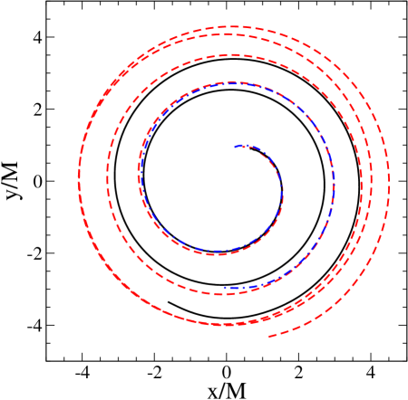
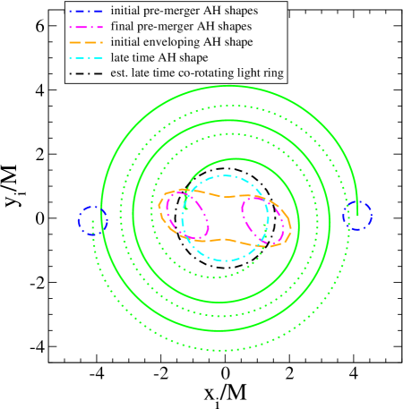
Figure 1: (left) The orbital motion of one BH from each of the three cases: the dot-dashed (blue) line is $d=13$, the solid (black) $d=16$ and the dashed (red) $d=19$. The position of the BH is defined as the center of its AH, and the curve ends once an encompassing horizon is found. The eccentricity present in the initial data is particularly evident for the $d=19$ case, though in part this is due to numerical error—see Fig. 5. To aid in the comparison each trajectory was rotated by a constant phase so that they coincide at a coordinate separation of $3M$. (right) The orbital motion of the BH’s from the d=16 simulation, showing the coordinate shapes of the AHs at several key moments. Also shown is the location of the co-rotating light ring of the final BH—see the discussion in Sec. VI.

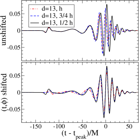
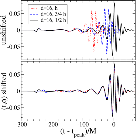
Figure 2: The ${\rm Re}[_{-2}C_{22}]$ component of the $d=13$ and $d=16$ waveforms, unshifted (top) and shifted (bottom). All resolutions are shown to demonstrate the size of numerical errors in the simulation, and data such as this was used to compute the errors for waveform quantities listed in Table 2.

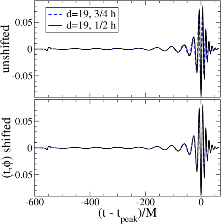
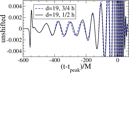
Figure 3: In the left panel we show the the ${\rm Re}[_{-2}C_{22}]$ component of the $d=19$ waveform, unshifted (top) and shifted (bottom). The lower resolution data for the $d=19$ case was accidentally deleted. In the right panel we zoom in for a close-up of the inspiral part of the unshifted waveform. From these two results alone it would appear as if the $d=19$ simulations have anomalously good convergence behavior (compare to Fig. 2). However, this is not the case—refer to the discussion in Sec. III.3, and see Figs. 4 and 5 for other estimators of the convergence of the solution.

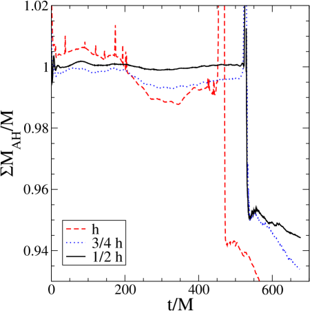
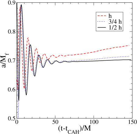
Figure 4: Sum of AH masses (left panel), and the Kerr angular momentum parameter of the final BH (right panel) for the $d=19$ simulations. The angular momentum was estimated using the ratio of polar to equatorial proper circumference of the horizon brandt_seidel ; the dynamical horizons estimate ashtekar_krishnan gives similar results modulo the oscillations about the mean. Except near the time of merger the sum of AH masses in the spacetime should be conserved, and similarly at late times for the Kerr parameter. As resolution increases we see the expected trends in these quantities. Note that the ”jaggies” in the AH mass estimate is a reflection of AH finder problems in the code, and not irregularities in the underlying solution FP3 .

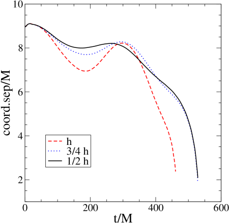
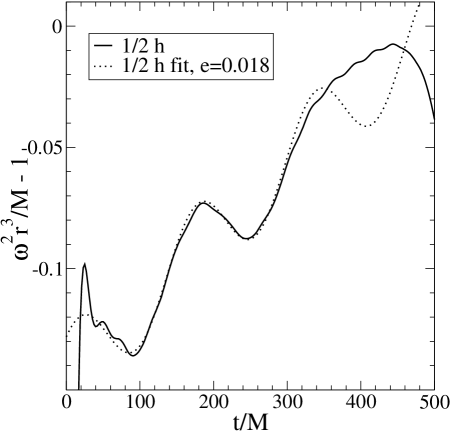
Figure 5: In the left panel we show the coordinate separation of the BHs as a function of time for the $d=19$ simulations. This plot highlights the eccentricity within the orbit and it also reflects the phasing behavior in the waveform for the $3/4h$ and $1/2h$ cases—see Fig. 3. In the right panel we estimate the eccentricity for the $d=19$ case: shown is a plot of the left hand side of Eq. (21) together with a fit of the form $a_{0}+a_{1}t+e\,\cos(a_{2}t+a_{3})$ to the early time behavior of this function. We estimate the eccentricity to be the amplitude of the sinusoidal part of the fitting function.

III.4 Diagnostic of the orbital evolution

The initial orbits of the $d=19$ case displayed in Fig. 1 are clearly neither circular nor a smooth adiabatic inspiral. It is natural to refer to such orbits as being eccentric. However, describing orbits as “eccentric” when radiative effects are strong can be problematic. The notion of eccentricity is precise in Newtonian physics, where the eccentricity is one of two parameters needed to describe a general, bound elliptic orbit. In general relativity, even when considering only the conservative dynamics, binaries do not follow closed elliptic orbits. When the dissipative effects of gravitational radiation are strong, it becomes even more difficult to define the concept of eccentricity.

The initial data we use starts with essentially no radial momentum. If radiative dissipation is neglected, such orbits can be circular or eccentric depending on the magnitude of the orbital angular velocity. But, because of radiation reaction, initial data with no radial momenum cannot represent a binary on a smooth quasi-circular inspiral. In fact, such an orbit must have some effective eccentricity.

We will use two methods to attempt to calculate this eccentricity in the $d=19$ case. Neither of these methods work well for the $d=13$ and $d=16$ cases as they do not exhibit enough orbital motion prior to merger. The first method uses the following relationship that holds for an orbit with eccentricity $e$, orbital angular frequency $\omega$ and separation $r$ in Newtonian theory:

$$\omega^{2}(t)\,r^{3}(t)/M-1=e\cos(\phi(t)).$$ (21)

Lower order general relativistic corrections (in particular perihelion precession) will change the argument to the cosine function, though the amplitude remains $e$. The right panel in Fig. 5 shows the LHS of Eq. (21) for the $d=19$ simulation, with $\omega$ and $r$ calculated from the coordinate motion of the BHs. A certain amount of eccentricity is due to numerical error, though the trend in the curves of Fig. 5 as resolution increases indicates that some amount of eccentricity does come from the initial data. The numerical data does not follow Eq. (21) too closely, though at early times there are clear oscillations about a line, and we will use the amplitude of these oscillations to define $e$. For a fitting function we use $a_{0}+a_{1}t+e\,\cos(a_{2}t+a_{3})$, and guided by Eq. (21), we define the amplitude of the oscillation to be the eccentricity. For the $1/2h$ run the fit gives $e=0.018\pm 0.003$, with the uncertainty calculated using the $1/2h$ and $3/4h$ data and assumed second order convergence.

For a second estimate of the eccentricity we use another Newtonian definition given in Ref. MW :

$$e=\frac{\sqrt{\omega_{p}}-\sqrt{\omega_{a}}}{\sqrt{\omega_{p}}+\sqrt{\omega_{a}}},$$ (22)

where $\omega_{p}$ is the frequency $\omega$ at a local maxima, and $\omega_{a}$ is the frequency at the following local minima. Using this definition, and the data for the $d=19$ case shown in Fig. 7, we get $e=0.012$ ($0.029,0.068$) for the $1/2h$ ($3/4h,h$) resolution runs. The rather large differences in the values calculated using the different resolutions means that the corresponding uncertainty in $e$ calculated using Eq. (22) is also large: $\pm 0.014$ (for the values quoted in Table 3 we restricted $e\geq 0$).

As mentioned in Sec. II, Refs. MW ; BIW have shown that 3PN estimates of eccentric orbits suggest the quasicircular initial data being used has some intrinsic eccentricity. From Fig. 2 of Ref. BIW , we find a 3PN estimate of $e\sim 0.01$ for the $d=19$ case. We note that this is remarkably close to the eccentricity estimate obtained via Eq. (22). However, despite this coincidence, we should be cautious in attributing the “eccentricity” observed in the orbit of the $d=19$ case to a non-vanishing eccentricity in the initial data. It is important to remember that the initial data are constructed to have vanishing radial velocity. As shown by Miller MM , initially circular orbits clearly lead to the kind of effective eccentric behavior seen in our numerical evolutions. A comparison of Fig. 4 of Ref. MM with Fig. 5 of this paper also shows striking similarity. It is clear that the initial data, through a combination of a vanishing initial radial velocity and possibly non-vanishing initial eccentricity, results in an evolution that exhibits some undesired eccentric behavior. However, it is not yet possible to determine which, if either, effect dominates.

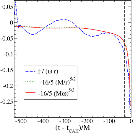
Figure 6: We plot the ratio between the radial velocity and the tangential velocity as evaluated in the numerical evolution of the $d=19$ case (dashed curve), and compare it with the Newtonian predictions (dot and continuous curves) obtained using the quadrupole formula. The two dashed vertical lines span the region in which a dynamical ISCO could be present.

Despite the presence of the eccentricity, the orbital motion on average is quasi-circular. By this we mean that throughout the evolution the radial velocity is smaller than the tangential velocity. At leading order, the quadrupole formula predicts for the radial velocity $\dot{r}=-16/5\,(M/r)^{3}$ and for the ratio between the radial and tangential velocity $\dot{r}/(\omega\,r)=-2/3\,\dot{\omega}/{\omega^{2}}=-16/5\,(M/r)^{5/2}=-16/5\,(M\omega)^{5/3}$, where we use $\omega^{2}\,r^{3}/M=1$. In Fig. 6 we show how the above relations are satisfied by the numerical simulations. For simplicity we only consider the high-resolution run $d=19$. Quite interestingly, the curves $-16/5\,(M/r)^{5/2}$ or $-16/5\,(M\omega)^{5/3}$ average the behavior of $\dot{r}/(\omega\,r)$ during the inspiral part and converge to it at later times. Between $30\mbox{--}50M$ before the formation of the CAH, we notice an abrupt change in the behavior of the ratio between the radial velocity and the tangential velocity, which suggests the presence of a blurred dynamical ISCO with subsequent plunge BD2 . Even during the plunge, the radial velocity is still much smaller than the tangential velocity, reaching the value of $20\%$ only at the end of the plunge. This result is a further confirmation that the numerical, equal-mass dynamics is quasi-circular until the end, as predicted by the EOB approach BD2 .

IV The inspiral

The analysis in Sec. III.4 has shown that, despite the presence of an initial eccentricity, the dynamics is quasi-circular. If the dynamics is sufficiently quasi-circular, then it should be possible to model the inspiral waveform and frequency using Newtonian and PN methods together with the quadrupole formula. In this section, we will compare the numerical waveforms to the expected results from Newtonian theory and PN theory LB assuming an adiabatic inspiral. In a subsequent section (Sec. VII) we will also consider the non-adiabatic EOB model BD1 ; BD2 ; DJS ; BD3 and Padé approximants DIS98 . Our analysis should be considered as a first-order attempt to assess the closeness of analytical and numerical results. More rigorous comparisons will be tackled in the future when numerical simulations start with initial conditions that more accurately model a binary on an adiabatic path closer to that describe by PN methods, and with simulations that have smaller or better understood systematic errors.

In addition to examining the full waveforms, it is useful to focus attention on the angular frequency of the waves and the underlying orbital motion. From the evolved data, there are several methods for determining the orbital angular frequency. The most direct measure is obtained by tracking the coordinate locations of the centers of the AHs of each individual BH. We label this measure of the frequency by $\omega_{c}$. Because it is based directly on generalized harmonic coordinate values, this measure of $\omega$ is susceptible to gauge effects. A second method for determining $\omega$ is to track the phase of the maximum of $\Psi_{4}$ in the equatorial plane as it intersects the extraction surface at $r=50M$. We denote the orbital angular frequency determined by this method by $\omega_{\lambda}$. Since the angular resolution at which $\Psi_{4}$ is sampled is coarser than the temporal resolution, we use spatial interpolation to find the phase $\phi_{\rm max}(t)$ of the maximum at time $t$, then smooth the curve in $t$ before computing $\omega_{\lambda}=d\phi_{\rm max}/dt$. As a third method, we note that if a complex signal $f(t)$ has a dominant frequency and it is circular polarized, then that frequency is given by ${\rm Im}[\dot{f}/f]$, where the dot ($\dot{\ }$) denotes a time derivative. In terms of the mode amplitudes ${}_{-2}C_{\ell m}(t,r)$, the dominant circular polarized frequency can be estimated by

$$\omega_{\rm Dm}=-\frac{1}{m}{\rm Im}\left[\frac{{{}_{-2}\dot{C}_{\ell m}}}{{}_{-2}C_{\ell m}}\right],$$ (23)

where we note that $m$ in this equation is the azimuthal index and should not be confused with the total mass. These different definitions of the frequency are summarized in Table 4.

Symbol	Type	Computed
$\omega_{c}$	orbital frequency	from AH centers (see Sec. IIB)
$\omega_{\lambda}$	${}_{-2}C_{22}$ frequency	by tracking wave peak (see Sec. IIB)
$\omega_{\rm Dm}$	${}_{-2}C_{lm}$ dominant (circular-polarized) frequency	from Eq. (23)
$\omega_{\rm NQC}$	${}_{-2}C_{22}$ Newtonian quasi-circular frequency	from Eq. (27)

Table 4: We summarize several frequency variables used in the text.

Figure 7 compares the orbital angular velocity $M\,\omega(t)$ obtained by these approaches, for the initial separations $d=16$ and $19$. First, note that various frequencies have been appropriately shifted in time to account for the wave propagation time to the extraction sphere. The initial numerical waveform is dominated by spurious radiation associated with the initial-data, and $\omega_{\lambda}$ and $\omega_{{\rm D}2}$ are quite noisy at early times. Though it is somewhat difficult to see in these plots, $\omega_{\lambda}$ and $\omega_{{\rm D}2}$ also extend to earlier times than does $\omega_{c}$. This is a manifestation of the fact that $\omega_{\lambda}$ and $\omega_{{\rm D}2}$ are obtained from information at the extraction sphere at $r=50M$. Also small and difficult to see, we note that there are unexpected deviations at early times in $\omega_{c}$. We find that all three measures of $\omega$ agree quite well except near the beginning of the evolution and near the end of the inspiral $30$–$40M$ before the time of the peak in $|\Psi_{4}|$.

The aberrant behavior of $\omega$ at early times is primarily due to the use of conformally-flat initial data and, consequently, to a lack of physically realistic initial radiative modes. This strongly affects $\omega_{\lambda}$ and $\omega_{D2}$. The small anomalous behavior in $\omega_{c}$ at early times might also be caused by artifacts in the initial data, and note that imposing spacetime harmonic coordinates at the initial time does create some “artificial” coordinate dynamics. Each of these methods for measuring $\omega$ are based directly on generalized harmonic coordinate values, and are susceptible to gauge effects. In particular, the coordinate position of an AH is certainly not a gauge-invariant quantity, and given that the BHs are in the strong-field region of the spacetime there is no a priori reason to expect the coordinate locations to have any simple mapping to what one may describe as the physical orbit. It is therefore somewhat surprising how well these “almost-harmonic” coordinates describe the orbit—more examples of this are given in the next section.

IV.1 Newtonian quadrupole approximation

Now consider a Newtonian binary in a circular orbit with orbital angular frequency $\omega$. For a binary with reduced mass $\mu=m_{1}m_{2}/M$ and mass ratio $\nu=\mu/M$, the standard quadrupole formula yields

$$rM\Psi_{4}=32\sqrt{\frac{\pi}{5}}\nu(M\omega)^{8/3}\left[e^{-2i(\omega t-\phi_{0})}{}_{-\!2}Y_{22}+e^{2i(\omega t-\phi_{0})}{}_{-\!2}Y_{2-\!2}\right]$$ (24)

where $\phi_{0}$ fixes the initial phase of the orbit and assuming right-handed rotation about the positive $z$-axis. If we replace $\omega t$ by the accumulated phase of the orbit

$$\phi(t)=\int_{0}^{t}{\omega(t^{\prime})dt^{\prime}},$$ (25)

then we find that we can approximate $\ell=2$ modes of the inspiral waveform by

$$_{-\!2}C_{2\pm\!2}(t)=32\sqrt{\frac{\pi}{5}}\,\nu\,[M\omega(t)]^{8/3}\,e^{\mp 2i(\phi(t)-\phi_{0})}.$$ (26)

Note that we have assumed an adiabatic inspiral and have replaced the constant orbital angular frequency $\omega$ of the circular orbit with a time-dependent orbital angular frequency $\omega(t)$. We refer to the result in Eq. (26) as the Newtonian quadrupole circular orbit (NQC) approximation.

This result can be used in two ways. First, if we assume that Eq. (26) provides a good approximation to the waveform, then we can extract $\omega(t)$ from the waveform via

$$M\,\omega(t)=\left(\frac{1}{32\nu}\sqrt{\frac{5}{\pi}}|{}_{-\!2}C_{2\pm\!2}(t)|\right)^{3/8}\,.$$ (27)

In Fig. 7 we have also plotted $\omega_{\rm NQC}$ obtained by the Newtonian quadrupole circular orbit approximation of Eq. (27). As noted previously, near the beginning of each evolution, artifacts from the initial data dominate the waveform and this leads to large inaccuracies in $\omega_{\lambda}$ and $\omega_{\rm D2}$. Similar inaccuracies at early time are also seen in $\omega_{\rm NQC}$. Near the end of the inspiral, when the orbital motion is no longer close to circular, we should not expect Eq. (27) to yield an accurate value for $M\omega$ and we see that the NQC method is systematically underestimating the value of $M\omega$.

The inconsistency of these methods for determining $\omega$ near the end of the inspiral should remind us that the very notion of “orbital angular frequency” becomes poorly defined after the formation of a common horizon. $\omega_{c}$ terminates near the end of the inspiral as a common horizon forms. The various methods agree quite well until about a quarter of an orbit before the formation of a common horizon (see Fig. 8 below). At this point, which we refer to as the “decoupling point”, $\omega_{c}$ separates from $\omega_{\lambda}$ and $\omega_{D2}$ and begins to rise more rapidly. Determining the precise point of decoupling is difficult due to numerical noise in the frequencies, but it seems to occur close to a value of $M\omega_{\rm dec}=0.15\pm 0.01$. Incidentally, this moment of decoupling also seems to coincide with the time the centers of the individual AH’s cross what we estimate to be the late time co-rotating light ring of the final BH (see Sec.VI). Finally, in Secs. IV.2 and VII, we will again examine the orbital angular frequency of the numerical models and find that $\omega$ from 3PN-adiabatic and EOB circular orbits agrees well with $\omega_{c}$.

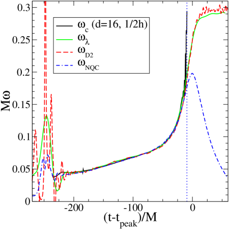
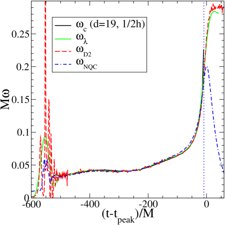
Figure 7: Orbital angular frequencies for the $d=16$ and $d=19$ cases evaluated using several different methods. The solid (black) line labeled $\omega_{c}$ displays $M\omega$ as determined from the coordinate locations of the center of each BH’s AH. The solid (green) line labeled $\omega_{\lambda}$ displays $M\omega$ as extracted by tracking the phase of the peak in $\Psi_{4}$ at an extraction surface placed at $r=50M$. The long-dash (red) line labeled $\omega_{\rm D2}$ displays the dominant frequency in ${}_{-2}C_{22}$ obtained using Eq. (23). The dash-dash-dot (blue) line labeled $\omega_{\rm NQC}$ displays the orbital angular velocity obtained from ${}_{-\!2}C_{22}(t)$ using Eq. (27). Finally, the vertical dotted (blue) line marks the approximate time that a common AH forms.

The second way that the NQC approximation can be used is to estimate ${}_{-\!2}C_{2\pm\!2}(t)$ by using $\omega$ extracted from the evolution. Figure 8 compares the real part of ${}_{-\!2}C_{22}(t)$ with the waveform estimated using the Newtonian quadrupole circular orbit approximation of Eq. (26) for both the $d=16$ and $19$ cases. In the upper half of each plot, we use $\omega_{c}$ for the orbital angular frequency. In the lower half of each plot, $\omega_{\lambda}$ is used. We do not consider reconstructing the waveform from $\omega_{\rm D2}$ or $\omega_{\rm NQC}$ because these where themselves derived from ${}_{-\!2}C_{22}(t)$.

A benefit of examining these plots is that they give a clear indication of how much of the initial waveform is contaminated by artifacts from the initial data. This can be most clearly seen in Fig. 8 in the comparison with $\omega_{c}$ where we find that the estimated waveform begins later than the extracted waveform. The reason is that $\omega_{c}$ is a function of “coordinate time” while the extracted waveform is a function of “retarded time” at the extraction radius. So, the beginning of the estimated waveform marks the earliest time that a waveform produced by the numerically evolved inspiral motion could begin. The numerical signal preceding this is due entirely to the unphysical initial radiative content of the initial data. This signal precedes the inspiral waveform because it originates from spatial locations in the domain that are closer than the binary to the extraction sphere. An initial segment of the true inspiral signal is also contaminated because of initial-data artifacts propagating to the extraction sphere from beyond the binary. If we make the reasonable assumption that the most significant contributions to the initial-data artifacts originate within the extraction sphere located at $r=50M$, then we should expect a total of around $2\times 50M$ of the signal to be contaminated as measured in the retarded time of the extraction sphere. This number cannot be exact since we expect the initial-data artifacts to be strongest close to the center of the extraction sphere, and also because of variations in the coordinate speed of light in the strong field region.

Both halves of the plots in Fig. 8 show a clear mismatch at early times. Because $\omega_{\lambda}$ is constructed from information at the extraction sphere, it shows an initial pulse of radiation that is clearly an artifact of the initial data. However, the level of contamination of the wavform decays quickly following this initial pulse and appears to have become insignificant by a time of $30M$ to $50M$ following this “initial-data pulse” .

A striking feature of these figures is the excellent agreement between the estimated and extracted waveforms following the initial contamination and up to a short time before the formation of a common AH. During this phase of the inspiral, Fig. 1 clearly shows that the motion of the binary is not circular. Nor is it the smooth adiabatic inspiral that we would expect from an astrophysical binary that has evolved from much larger separation. In fact, the observed motion exhibits a small radial oscillation about this “desired” motion. This effect is most easily seen in the longer $d=19$ evolution, and also in the plots of $\omega$ in Fig. 7 (see also Fig. 5, and Fig. 10 which includes a fit to the PN form for $\omega$ expected for adiabatic inspiral from large separation). The point we want to emphasize is that Eq. (26) gives an excellent approximation for the waveform, even when the motion is clearly non-circular, so long as the phase $\phi(t)$ and orbital angular velocity $\omega(t)$ accurately incorporate the non-circular aspects of the orbital motion. As mentioned above, the NQC approximation appears to work quite well up until about $1/4$ of an orbit (half a full wave cycle) before the appearance of a common horizon.

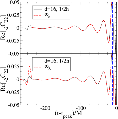
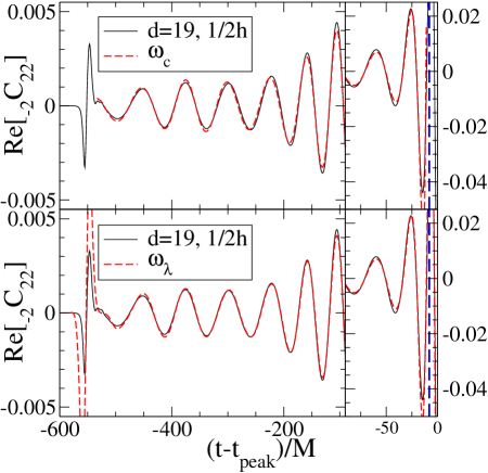
Figure 8: Comparison of numerical and NQC inspiral waveforms for the $d=16$ and $19$ cases. In all plots, the solid (black) line displays ${}_{-\!2}C_{22}(t)$ from the numerical waveform and the vertical long-dashed (blue) line marks the approximate time that a common AH forms. In the upper plots, the dashed (red) line displays ${}_{-\!2}C_{22}(t)$ as computed from Eq. (26) using $\omega_{c}$ and $\phi(t)$ is obtained from Eq. (25). In the lower plots, the dashed (red) line displays ${}_{-\!2}C_{22}(t)$ as computed from Eq. (26) using $\omega_{\lambda}$. The longer evolution of the $d=19$ run leads to significant changes in scale for ${}_{-\!2}C_{22}(t)$. Therefore, we change scales for the final $90M$ of the evolution.

Another rather intriguing example demonstrating the adequacy of the quadrupole formula, and how well adapted the numerical coordinate system is in describing the binary motion is shown in Fig. 9. For brevity we focus on a single example here, comparing the real part of the ${}_{-2}C_{22}$ component of the $d=19$ waveform to the same component of a waveform calculated using the quadrupole formula  for two point sources of mass $M/2$ following trajectories given by the coordinate locations of the AH’s from the simulation. The latter curve ends when a common AH forms, and has again been shifted in time by a constant amount to account for the propagation time for the wave to reach the extraction surface. The difference between this comparison and the preceding NQC comparison is we have not assumed circular orbits, using instead the detailed orbit motion obtained from the simulation. Not only does the good agreement testify to the well-suited nature of the coordinates, it shows that the quadrupole formula does a remarkably good job of capturing the dominant physics of GW emission during the entire merger regime prior to common AH formation.

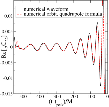
Figure 9: Comparison of the real part of the ${}_{-2}C_{22}$ component of the waveform from the $d=19$ ($h/2$) numerical simulation (solid curve) versus the same quantity calculated by using the quadrupole formula (dashed curve) for two point particles, each of mass $M/2$ and following trajectories given by the coordinate motion of the AH’s in the simulation (see Fig. 1). The waveform from the orbit ends once a common AH forms.

IV.2 Adiabatic post-Newtonian model

The post-Newtonian approximation to the two-body dynamics of compact objects provides the most accurate predictions for the motion and the GW emission during the inspiral phase, when the weak-field and slow-motion assumptions hold.

In a more rigorous analysis we would compare the numerical and analytical dynamical quantities expressed in the same coordinate system and gauge. Here and in Appendix B, we limit the comparison to a few gauge-invariant dynamical quantities, such as the orbital frequency $\omega$, the orbital phase $\phi$, the energy flux $F_{E}$ and the angular-momentum flux $F_{J}$, expressed in terms of the instantaneous orbital frequency and/or the time of a stationary observer at infinity. This is also motivated by the fact that previous studies DIS98 ; BD2 have shown that PN-approximants to dynamical quantities are more robust (under change of PN order) if expressed in terms of gauge-invariant quantities, notably the instantaneous orbital-frequency $M\omega$. At the present time, PN calculations provide the orbital frequency through 3.5PN order 35PNnospin if spins are neglected, and through 2.5PN order 25PNspin if spins are included. As mentioned in Sec. II and shown in Table 1, the numerical initial data describe BHs which carry a small spin aligned with the direction of the orbital angular-momentum $\ell$. For this reason we include spin effects in the PN approximants.

In this section we limit the analysis to the so-called PN-adiabatic model. In Sec. VII we shall investigate the comparisons with the EOB model which goes beyond the adiabatic approximation. In the PN-adiabatic model the waveforms are computed assuming that the motion proceeds along an adiabatic sequence of quasi-circular orbits. More specifically, one assumes $\dot{r}=0$ and evaluates the variation in time of the orbital frequency $\omega$ from the energy-balance equation $dE/dt=-F_{E}$, where $E$ is the two-body energy and $F_{E}$ is the GW energy flux. In particular, $E$ and $F_{E}$ are first computed for circular orbits and written as a power expansion in $M\,\omega$, then $\dot{\omega}(t)=-F_{E}(\omega)/(dE(\omega)/d\omega)$. The adiabatic sequence of circular orbits ends at the conservative Innermost Circular Orbit (ICO), i.e., the ICO evaluated from the conservative dynamics by imposing ${(dE/d\omega)}{{}_{\rm ICO}}=0$ LB . The study of Ref. BD2 (see in particular Figs. 4 and 5 and discussion around them) and Ref. MM , showed that waveforms computed in the adiabatic approximation (which are very accurate at large separations) can have a non-negligible phase difference with respect to waveforms computed in the non-adiabatic approximation, even before reaching the last stable orbit. The accuracy of our numerical simulations and the nature of the initial data will not allow us to explore these phase differences. Nevertheless, we have found it useful to use the adiabatic PN model as a diagnostic of the last few cycles of the numerical evolution.

As discussed in Sec. IV.1, it takes a certain time for the evolution to settle to a quasi-circular orbit. Moreover, the numerical results contain a non-negligible amount of eccentricity. For these reasons we shall evaluate the PN-adiabatic approximant which best averages the numerical orbital frequency until either the dynamical ISCO, the decoupling frequency, or the CAH. Again, these issues will be overcome when numerical simulations starting at larger separation, and from initial conditions that more accurately model an adiabatic inspiral, become available. We notice that in principle there could be non-negligible differences between the instantaneous orbital frequency as defined in PN theory and in the numerical simulation. In the latter, the orbital angular frequency is calculated from the coordinate locations of the centers of the AHs of each individual BH. However, since in Sec. IV.2 we have found that the numerical orbital-frequency agrees quite well with the numerical GW frequency extracted at larger radii, we expect that the differences are small.

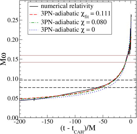
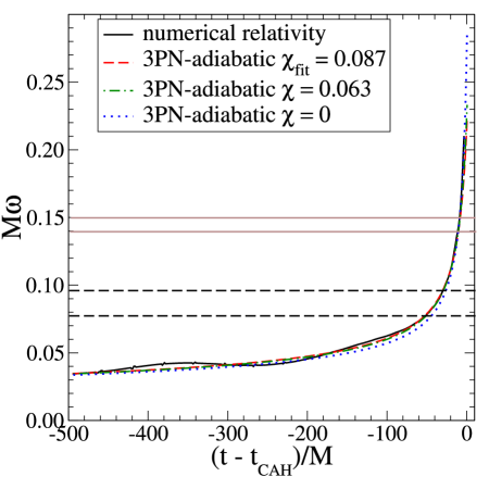
Figure 10: We compare the NR and three analytical orbital frequencies obtained by fitting (i) both $t_{c}$ and $\chi$ (dashed line), (ii) only $t_{c}$ and using the nominal $\chi$ value from Table 1 (dot-dashed line) and (iii) only $t_{c}$ and assuming $\chi=0$ (dot line). The left panel refers to the run $d=16$, the right panel to $d=19$. From top to bottom, the continuous horizontal lines mark the ICO frequencies as predicted by the 3PN-adiabatic energy and the decoupling frequency. The dashed horizontal line in the right panel span the frequency range when a dynamical ISCO could be present.

Defining $\tau=\nu\,(t_{c}-t)/5M$, where $t_{c}$ is the time at which the orbital-frequency diverges (time of coalescence, not to be confused with the decoupling time) we have

$$M\,\omega = {1\over 8}\tau^{-3/8}\biggl{\{}1+\left(\frac{743}{2688}+\frac{11}{32}\nu\right)\tau^{-1/4}-\frac{3}{10}\pi\tau^{-3/8}$$ (28)

$$+ \left(\frac{47}{40}\,\frac{S_{\ell}}{M^{2}}+\frac{15}{32}\frac{\delta M}{M}\,\frac{\Sigma_{\ell}}{M^{2}}\right)\,\tau^{-3/8}$$

$$+ \left(\frac{1855099}{14450688}+\frac{56975}{258048}\nu+\frac{371}{2048}\nu^{2}\right)\tau^{-1/2}+\left(-\frac{7729}{21504}+\frac{13}{256}\nu\right)\pi\tau^{-5/8}$$

$$+ \left[\left(\frac{101653}{32256}+\frac{733}{896}\nu\right)\,\frac{S_{\ell}}{M^{2}}+\left(\frac{7453}{7168}+\frac{347}{896}\nu\right)\,\frac{\delta M}{M}\,\frac{\Sigma_{\ell}}{M^{2}}\right]\,\tau^{-5/8}$$

$$+ \left(-\frac{720817631400877}{288412611379200}+\frac{53}{200}\pi^{2}+\frac{107}{280}C-\frac{107}{2240}\ln\left(\frac{\tau}{256}\right)\right.$$

$$+ \left.\left[\frac{25302017977}{4161798144}-\frac{451}{2048}\pi^{2}\right]\nu-\frac{30913}{1835008}\nu^{2}+\frac{235925}{1769472}\nu^{3}\right)\tau^{-3/4}$$

$$+ \left(-\frac{188516689}{433520640}-\frac{97765}{258048}\nu+\frac{141769}{1290240}\nu^{2}\right)\pi\tau^{-7/8}\biggr{\}}\;,$$

where $\delta M=m_{1}-m_{2}$, the spin variables are

$$\mathbf{S}\equiv\mathbf{S}_{1}+\mathbf{S}_{2}\,,$$ (29)

$$\mathbf{\Sigma}\equiv M\left[\frac{\mathbf{S}_{2}}{m_{2}}-\frac{\mathbf{S}_{1}}{m_{1}}\right]\,,$$ (30)

with $\mathbf{S}_{i}=\chi_{i}\,m_{i}^{2}\,\hat{\mathbf{S}}_{i}$. In Eq. (28) we have denoted with $S_{\ell}$ and $\Sigma_{\ell}$ the spin components along the direction of the orbital angular-momentum $\ell$ 25PNspin . The orbital phase through 3.5PN order reads

$$\phi = \phi_{0}-{1\over\nu}\biggl{\{}\tau^{5/8}+\left(\frac{3715}{8064}+\frac{55}{96}\nu\right)\tau^{3/8}-\frac{3}{4}\pi\tau^{1/4}$$ (31)

$$+ \left(\frac{47}{16}\,\frac{S_{\ell}}{M^{2}}+\frac{75}{64}\frac{\delta M}{M}\,\frac{\Sigma_{\ell}}{M^{2}}\right)\,\tau^{1/4}$$

$$+ \left(\frac{9275495}{14450688}+\frac{284875}{258048}\nu+\frac{1855}{2048}\nu^{2}\right)\tau^{1/8}+\left(-\frac{38645}{172032}+\frac{65}{2048}\nu\right)\pi\ln\left({\tau}\right)$$

$$+ \left[\left(\frac{508265}{258048}+\frac{3665}{7168}\nu\right)\,\frac{S_{\ell}}{M^{2}}+\left(\frac{37265}{57344}+\frac{1735}{7168}\nu\right)\,\frac{\delta M}{M}\,\frac{\Sigma_{\ell}}{M^{2}}\right]\,\ln\left({\tau}\right)$$

$$+ \left(\frac{831032450749357}{57682522275840}-\frac{53}{40}\pi^{2}-\frac{107}{56}C+\frac{107}{448}\ln\left(\frac{\tau}{256}\right)\right.$$

$$+ \left.\left[-\frac{126510089885}{4161798144}+\frac{2255}{2048}\pi^{2}\right]\nu+\frac{154565}{1835008}\nu^{2}-\frac{1179625}{1769472}\nu^{3}\right)\tau^{-1/8}$$

$$+ \left(\frac{188516689}{173408256}+\frac{488825}{516096}\nu-\frac{141769}{516096}\nu^{2}\right)\pi\tau^{-1/4}\biggr{\}}\;,$$

where $C=0.577\cdots$ is the Euler constant and $\phi_{0}$ is an arbitrary constant. The non-spin terms in Eqs. (28) and (31) are given by Eqs. (12) and (13) of Refs. BFIJ ; 35PNnospin , while we evaluated the spin terms through 2.5PN order using the recent results of Ref. 25PNspin (we use the constant spin variables as defined in Ref. 25PNspin ), and we neglected spin-spin contributions.

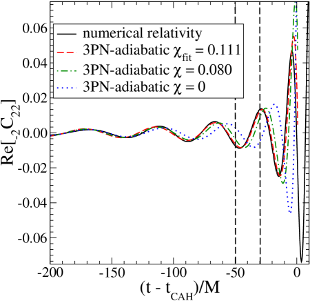
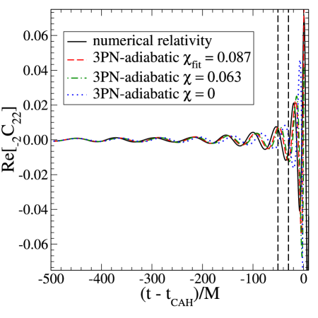
Figure 11: We compare the NR and analytical ${\rm Re}[{}_{-2}C_{22}]$ obtained by fitting the orbital frequencies. The fit is done for (i) both $t_{c}$ and $\chi$ (dashed line), (ii) only for $t_{c}$ and using the nominal value for $\chi$ from Table 1 (dot-dashed line) and (iii) only for $t_{c}$ and assuming $\chi=0$ (dot line). The left panel refers to the run $d=16$, the right panel to $d=19$. The dashed vertical lines span the region during which a dynamical ISCO could be present. The waveform cycle beyond this point could be associated with the plunge cycle.

For each of the three runs, we determine the time of coalescence $t_{c}$ and the spin-magnitude $\chi=\chi_{1}=\chi_{2}$ by fitting the PN orbital frequency $(\ref{omega})$ to the numerical orbital frequency $\omega_{c}$ using a non-linear least-squares method. Figure 10 shows the results for $d=16$ and $d=19$. Due to the initial burst of radiation related to the initial conditions, we remove from the numerical data the first $\approx 22M$ and $\approx 34M$, for the $d=16$ and $d=19$ runs, respectively. In Sec. III.4 we discussed the possible presence of a blurred dynamical ISCO BD2 occurring $30\mbox{--}50M$ before the CAH forms, at $M\,\omega_{\rm dyn\,ISCO}=0.078\mbox{--}0.097$. The orbital frequency at the conservative ICO evaluated at 3PN order with $\chi=0.080$ is $M\,\omega_{\rm ICO}=0.143$ and with $\chi=0.063$ is $M\,\omega_{\rm ICO}=0.140$. We mark all these frequencies in Fig. 10 along with the decoupling frequency. In principle, the adiabatic PN waveform should be used only until the last stable orbit, since it was derived from the balance equation for circular orbits which ends at this last stable orbit. However, since the two-body motion predicted by the numerical simulations is rather adiabatic and quasi-circular until the CAH forms BD2 , we extend the PN waveforms through the plunge until almost that point. More specifically, we fit until the time at which the numerical orbital frequency decouples from the GW frequency, $M\omega_{\rm dec}\approx 0.15\pm 0.01$. Notice that by fitting the time of coalescence $t_{c}$ and $\chi$ we are fitting the initial value of the orbital frequency. We find that the 3PN-approximant best fits the data with $\chi^{\rm d=16}=0.111$ and $t_{c}^{\rm d=16}=220.1\,M$ [$M\,\omega(t=0)=0.04789$], $\chi^{\rm d=19}=0.0874$ and $t_{c}^{\rm d=19}=509.1\,M$ [$M\,\omega(t=0)=0.03477$]. If we fit until the CAH time, we find $\chi^{\rm d=16}=0.0812$ and $t_{c}^{\rm d=16}=217.6\,M$ [$M\,\omega(t=0)=0.04715$], $\chi^{\rm d=19}=0.0626$ and $t_{c}^{\rm d=19}=506.2\,m$ [$M\,\omega(t=0)=0.03447$]. Those values are closer to the nominal $\chi$ values of Table 1. However, we think this is accidental. Finally, notice that if we fit until the dynamcal ISCO $M\omega_{\rm dyn\,ISCO}=0.096$ we find $\chi^{\rm d=19}=0.113$ and $t_{c}^{\rm d=19}=514.3\,M$ [$M\,\omega(t=0)=0.03502$].

In Fig. 10 we also show curves evaluated using the nominal $\chi$ value of Table 1. To understand how spins affect the PN-adiabatic orbital frequency, we show in Fig. 10 also the case in which we fix $\chi=0$ and fit only $t_{c}$. The latter values produce a difference of $\approx 0.3$ GW cycles at the CAH time with respect to the case where we fit both $t_{c}$ and $\chi$. Although we can use the numerical results to discriminate between several PN-adiabatic models with spin, it is not clear which role the spin variable is playing in fitting the data. In fact, the spin values obtained from the fit are also affected by the eccentricity present in the numerical data but absent in the analytical model.

Using the time of coalescence and spin values obtained from the fits, we plot in Fig. 11 the waveforms ${\rm Re}[{}_{-2}C_{22}]$. Notice that the GW phase differences between the fitted models is smaller than the maximum GW phase error estimated in Table 3 using lower resolution runs. This gives a concrete example of how cumulative phase error in a numerical simulation translates to uncertainties associating PN model parameters with the numerical waveform, despite the deceptively small phase error after maquillage. PN-adiabatic models can also fit the data of lower resolution runs and give initial orbital frequencies larger than those found for the high resolution runs.

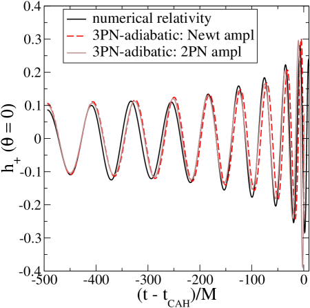
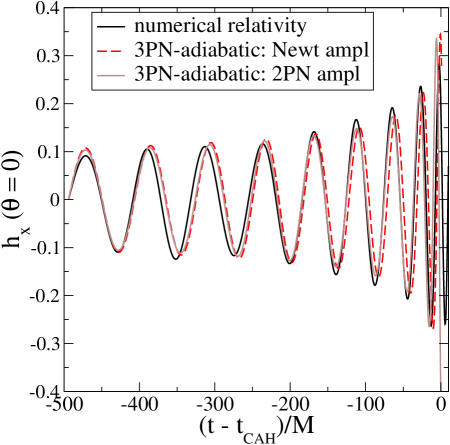
Figure 12: We plot the numerical $h_{+}$ (left panel) and $h_{\times}$ (right panel) extracted along the direction perpendicular to the orbital plane (dark continuous line) and compare them with PN-adiabatic predictions with the phase evaluated at 3PN order and the amplitude evaluated either at Newtonian order (dashed line) or through 2PN order (light continuous line). These results refer to the $d=19$ run.

So far, when comparing with numerical waveforms, we have neglected higher-order PN corrections to the GW amplitude and have restricted the comparison to ${\rm Re}[{}_{-2}C_{22}]$, i.e., we used waveforms in the so-called restricted approximation. In Ref. BIWW the authors evaluated the ready-to-use PN waveforms $h_{+}$ and $h_{\times}$ through 2PN order in the amplitude (see Ref. ABQI where this computation has been pushed through 2.5PN order). In Figs. 12 we compare the numerical $h_{+}$ and $h_{\times}$, which are obtained by integrating $\psi_{4}$ twice in time, with the analytical $h_{+}$ and $h_{\times}$ as given by Eqs. (2)–(4) of Ref. BIWW . The phase is computed from Eq. (31) at 3PN order with the values of $t_{c}$ and $\chi$ obtained from the best fit. The waves are extracted along the direction perpendicular to the orbital plane. Because the BH masses are equal, only the $2^{\rm nd}$ harmonic is present. We would conclude that higher-order PN amplitude corrections have a mild effect in the waveform emitted by equal-mass binaries. However, we notice an oscillating behavior in the PN approximation to $h_{+}$ and $h_{\times}$. For example the 1PN correction is rather large and opposite in sign to the Newtonian correction, resulting in a significant reduction of the amplitude of the signal. The 1.5PN and 2PN corrections undo this effect. This oscillating behavior seems to also affect the higher multipoles $C_{lm}$. In fact, we checked that $C_{44}$ is well approximated by the 3PN-adiabatic model for the phase, if computed at (leading) 1PN order in the amplitude, but the agreement become worse when 2PN corrections are added. We plan to investigate in more detail the effect of higher-order PN corrections and higher multipoles in the future.

To obtain more robust comparisons between PN and numerical predictions, it would be preferable to start the numerical evolution where we are confident that the PN expansion can be safely applied. First, we notice that if we were computing $\omega$ as a function of time instead of from Eq. (28), then integrating numerically the following equation 35PNnospin ; 25PNspin

$$\frac{\dot{\omega}}{\omega^{2}}=\frac{96}{5}\,\nu\,(M\omega)^{5/3}\Bigg{\{}1-\frac{743+924\,\nu}{336}\,(m\omega)^{2/3}+\frac{(M\omega)}{M^{2}}\left[-\frac{47}{3}S_{\ell}-\frac{25}{4}\frac{\delta M}{M}\Sigma_{\ell}\right]+4\pi(M\omega)$$

$$+\Bigg{(}\frac{34\,103}{18\,144}+\frac{13\,661}{2\,016}\,\nu+\frac{59}{18}\,\nu^{2}\Bigg{)}\,(M\omega)^{4/3}+\frac{(M\omega)^{5/3}}{M^{2}}\left[\left(-\frac{31811}{1008}+\frac{5039}{84}\nu\right)S_{\ell}+\left(-\frac{473}{84}+\frac{1231}{56}\nu\right)\frac{\delta M}{M}\Sigma_{\ell}\right]$$

$$-\frac{1}{672}\,(4\,159+15\,876\,\nu)\,\pi\,(M\omega)^{5/3}+\Bigg{[}\left(\frac{16\,447\,322\,263}{139\,708\,800}-\frac{1\,712}{105}\gamma_{E}+\frac{16}{3}\pi^{2}\right)+\left(-\frac{56\,198\,689}{217\,728}+\frac{451}{48}\pi^{2}\right)\nu$$

$$+\frac{541}{896}\nu^{2}-\frac{5\,605}{2\,592}\nu^{3}-\frac{856}{105}\log\left[16(M\omega)^{2/3}\right]\Bigg{]}(M\omega)^{2}+\Bigg{(}-\frac{4\,415}{4\,032}+\frac{358\,675}{6\,048}\,\nu+\frac{91\,495}{1\,512}\,\nu^{2}\Bigg{)}\,\pi\,(M\omega)^{7/3}\Bigg{\}}\,,$$ (32)

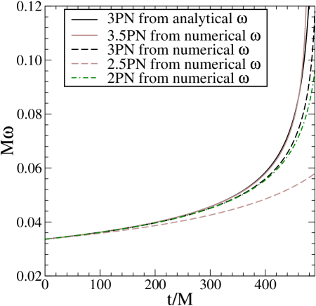
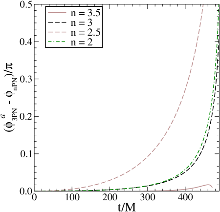
Figure 13: In the left panel we plot the orbital frequency for several PN approximants computed from Eqs. (28) and (32) whose frequencies coincide at time $t=0$. In the right panel we plot the differences between the number of GW cycles at 3PN computed from the analytical Eq. (28), and at nPN order computed from Eq. (32). The initial frequency coincides with the one computed from the fit of the $d=19$ run when $\chi=0$.

which can be derived expanding $\dot{\omega}=-F(\omega)/(dE/d\omega)$ in powers of $(M\omega)$, we find some differences from Eq. (28). In particular, at 3.5PN and 2.5PN orders, $\omega$ derived from Eq. (28) reaches a maximum and then starts decreasing, becoming negative. By contrast, this behavior does not occur in the $\omega$ derived by numerically integrating Eq. (32). In Fig. 13 we show the differences in the orbital frequency and the number of GW cycles if the latter quantities were computed from Eq. (32) at different PN orders but with the same initial frequency $\omega_{0}=0.03361$. We consider here a non-spinning binary. In the right panel of Fig. 13 we compute the differences in the number of GW cycles between the 3PN $\omega$ from the analytical Eq. (28) and several PN $\omega$ from Eq. (32). Quite interestingly the 3.5PN order computed numerically is very close to the 3PN order computed analytically, whereas the 3.5PN order computed analytically has almost half a cycle of difference at the end of the inspiral. These differences are a consequence of the fact that at such (close) initial separation, $M\,\omega\sim 0.033$, the differences between PN-approximants are not negligible. This fact is better illustrated in Fig. 14. We start the evolutions at $M\,\omega=0.004$ (left panel) and $M\,\omega=0.02$ (right panel) and plot the differences between the number of GW cycles at 3.5PN and at nPN order versus the $\omega$ computed at 3.5PN order. All quantities are obtained by numerically integrating Eq. (28) with spins set to zero. 2PN and 2.5PN approximants accumulate large differences from the 3.5PN-approximant when evolving from larger separations (left panel).

Thus, summarizing, the phase computed at 3PN order from Eq. (28) or at 3.5PN order from Eq. (32) best-fit the numerical results. If we wanted to investigate to which PN order, notably 3PN or 3.5PN, the NR orbital frequency is closest to, we would need to start the numerical evolution at frequencies smaller then the one used in the $d=19$ run, which is $\sim 0.033$.

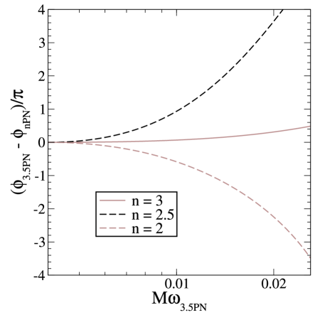
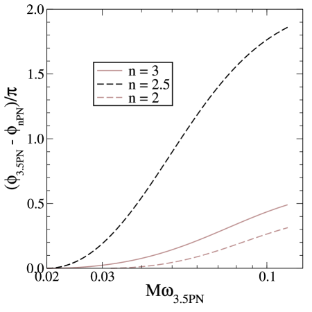
Figure 14: We plot the differences between the number of GW cycles at 3.5PN and at nPN order versus the 3.5PN $\omega$. All quantities are computed integrating numerically Eq. (32) with spins set to zero. The initial and final frequencies are $M\omega=0.004$ and $M\omega=0.026$ in the left panel, $M\omega=0.02$ and $M\omega=0.13$ in the right panel. They correspond to an equal-mass binary sweeping in the most sensitive frequency band of LIGO from $\sim 43$ Hz to $\sim 280$ Hz of mass $(3+3)M_{\odot}$ in the left panel and of mass $(15+15)M_{\odot}$ in the right panel.

V The ring-down phase

During the ring-down, the GW can be decomposed in terms of the quasi-normal modes (QNM) of KerrL85 ; E89 ; brandt_seidel . These modes are distinguished by their longitudinal and azimuthal indices $\ell$ and $m$, as well as by their overtone number $n$. Each mode has a particular frequency $\omega_{\ell mn}$ and decay constant $\tau_{\ell mn}$ which are functions of the Kerr parameter $a$ and total mass $M_{f}$ of the background BH that is being perturbed. To shorten the notation, we will introduce the complex frequency $\hat{\omega}_{\ell mn}$ and use ^∗ to denote complex conjugation:

$$\hat{\omega}_{\ell mn}\equiv\omega_{\ell mn}-i/\tau_{\ell mn}.$$ (33)

Following Ref. BCW , the ring down can be expressed, in terms of the Weyl scalar as

$$rM\Psi_{4} = \sum_{\ell mn}\Bigl{\{}{\cal C}_{\ell mn}e^{-i(\hat{\omega}_{\ell mn}t+\phi_{\ell mn})}S_{\ell mn}+{\cal C}^{\prime}_{\ell mn}e^{i(\hat{\omega}^{*}_{\ell mn}t+\phi^{\prime}_{\ell mn})}S^{*}_{\ell mn}\Bigr{\}},$$ (34)

where ${\cal C}_{\ell mn}$, ${\cal C}^{\prime}_{\ell mn}$, $\phi_{\ell mn}$, and $\phi^{\prime}_{\ell mn}$ are real constants, and $S_{\ell mn}=S_{\ell m}(a\hat{\omega}_{\ell mn})$ are the spin-weight -2 spheroidal harmonics implicitly evaluated at the complex QNM frequencies. The primed terms are necessary because, for a given $(\ell,m,n)$ and a fixed non-vanishing angular momentum, there are two solutions of the eigenvalue problem. To make the notation as clear as possible, we will always take the real frequencies and decay constants to be non-negative, so $\omega_{\ell mn}\geq 0$ and $\tau_{\ell mn}\geq 0$. Of the two solutions to the eigenvalue problem for fixed $(\ell,m,n)$, one solution has positive frequency and one negative, and the complex frequencies are related by $-\hat{\omega}_{\ell mn}=\hat{\omega}^{*}_{\ell-\!mn}$ (see Ref. BCW for a full discussion). Because of this relationship, it is only necessary to determine the positive (or negative) frequency modes. In Ref. BCW the authors compute the positive frequency modes and choose the convention that $\omega_{\ell mn}\geq\omega_{\ell-\!mn}$, with equality in the case that $m=0$ or $a=0$. Finally, we note that with these conventions, it is necessary to introduce an overall sign change on the real frequency in the equations of Ref. BCW in order for the signs of the frequencies of the various modes to agree with numerical simulations.

The decomposition of $\Psi_{4}$ in terms of spin-weight -2 spherical harmonics is given by Eq. (17). In order to relate the expansion coefficients in Eqs (34) and (17), we need the expansion of the spheriodal harmonics in terms of the spherical harmonics. Following Press and Teukolsky PT ,

$$S_{\ell mn}=\sum_{\ell^{\prime\prime}}{\cal A}_{\ell\ell^{\prime\prime}mn}{}_{-\!2}Y_{\ell^{\prime\prime}m}.$$ (35)

Using the orthonormality of spin-weighted spherical harmonics, we find that

$${}_{-\!2}C_{\ell m} = \sum_{\ell^{\prime\prime}n}\Bigl{\{}{\cal C}_{\ell^{\prime\prime}mn}{\cal A}_{\ell\ell^{\prime\prime}mn}e^{-i(\hat{\omega}_{\ell^{\prime\prime}mn}t+\phi_{\ell^{\prime\prime}mn})}+{\cal C}^{\prime}_{\ell^{\prime\prime}-\!mn}{\cal A}^{*}_{\ell\ell^{\prime\prime}-\!mn}e^{i(\hat{\omega}^{*}_{\ell^{\prime\prime}-\!mn}t+\phi^{\prime}_{\ell^{\prime\prime}-\!mn})}\Bigr{\}},$$ (36)

$$\equiv \sum_{\ell^{\prime\prime}n}\Bigl{\{}{\cal C}_{\ell\ell^{\prime\prime}mn}e^{-i(\hat{\omega}_{\ell^{\prime\prime}mn}t+\phi_{\ell\ell^{\prime\prime}mn})}+{\cal C}^{\prime}_{\ell\ell^{\prime\prime}mn}e^{i(\hat{\omega}^{*}_{\ell^{\prime\prime}-\!mn}t+\phi^{\prime}_{\ell\ell^{\prime\prime}mn})}\Bigr{\}}.$$ (37)

So, in principle, a spherical harmonic mode amplitude ${}_{-\!2}C_{\ell m}$ of the ring-down signal can contain a contribution from any of the negative frequency modes with azimuthal index $m$ and from any of the positive frequency modes with azimuthal index $-m$. Note that in the second version of this expansion, the complex coefficients ${\cal A}_{\ell\ell^{\prime\prime}mn}$ have been absorbed into the new real expansion coefficients ${\cal C}_{\ell\ell^{\prime\prime}mn}$, ${\cal C}^{\prime}_{\ell\ell^{\prime\prime}mn}$, $\phi_{\ell\ell^{\prime\prime}mn}$, and $\phi^{\prime}_{\ell\ell^{\prime\prime}mn}$, where each coefficient now has four indices.

The expansion coefficients ${\cal A}_{\ell\ell^{\prime\prime}mn}$ depend on the product of the Kerr parameter and the complex QNM frequency $a\hat{\omega}_{\ell mn}$ and for sufficiently small values can be determined via perturbation theory (cf. Ref. PT ). For example, using first order perturbation theory, we find

$${}_{-\!2}C_{22} = \sum_{n}\Bigl{\{}{\cal C}_{22n}e^{-i(\hat{\omega}_{22n}t+\phi_{22n})}+{\cal C}^{\prime}_{2-\!2n}e^{i(\hat{\omega}^{*}_{2-\!2n}t+\phi^{\prime}_{2-\!2n})}$$ (42)

$$\mbox{}\hskip 18.06749pt+\frac{1}{18}\sqrt{\frac{5}{7}}a\hat{\omega}_{32n}(4+a\hat{\omega}_{32n}){\cal C}_{32n}e^{-i(\hat{\omega}_{32n}t+\phi_{32n})}$$

$$\mbox{}\hskip 18.06749pt-\frac{1}{18}\sqrt{\frac{5}{7}}a\hat{\omega}^{*}_{3-\!2n}(4+a\hat{\omega}^{*}_{3-\!2n}){\cal C}^{\prime}_{3-\!2n}e^{i(\hat{\omega}^{*}_{3-\!2n}t+\phi^{\prime}_{3-\!2n})}$$

$$\mbox{}\hskip 18.06749pt+\frac{\sqrt{5}}{294}(a\hat{\omega}_{42n})^{2}{\cal C}_{42n}e^{-i(\hat{\omega}_{42n}t+\phi_{42n})}$$

$$\mbox{}\hskip 18.06749pt+\frac{\sqrt{5}}{294}(a\hat{\omega}^{*}_{4-\!2n})^{2}{\cal C}^{\prime}_{4-\!2n}e^{i(\hat{\omega}_{4-\!2n}t+\phi^{\prime}_{4-\!2n})}\Bigr{\}}.$$

We have extracted the various QNM contributions to the ${}_{-\!2}C_{22}(t)$ ring-down signal in the following way . At late times, we expect the $\ell=2$, $m=2$, $n=0$ QNM to dominate. We fit the signal after time $t_{r}+t_{\rm peak}$ to this single mode using non-linear regression and choose $t_{r}$ to minimize the error in the fit. There are four dimensionless parameters in this non-linear fit: ${\cal C}_{220}$, $\phi_{220}$, $m\omega_{220}$, and $\tau_{220}/m$. However, instead of fitting directly for these four parameters, we treat $m\omega_{\ell mn}$ and $\tau_{\ell mn}/m$ as functions of $a/M_{f}$ and $M_{f}/m$ which can be obtained via interpolation from tabulated values (cf. Tables II–IV of Ref. BCW ) or via approximating functions (cf. Tables VIII–X of Ref. BCW ). The advantage of using $(a/M_{f},M_{f}/m,{\cal C}_{220},\phi_{220})$ for the set of fitting parameters comes when we fit to additional modes.

If we knew $a/M_{f}$ and $M_{f}/M$ precisely from the fit to the dominant mode, then we could directly compute the values for $M\omega_{\ell mn}$ and $\tau_{\ell mn}/M$ for all additional contributing modes. All that would be necessary for determining the contribution of each additional mode would be to fit for its amplitude and phase. However, we will not know $a/M_{f}$ and $M_{f}/M$ precisely from the fit to the dominant mode. Therefore, we treat the frequency and damping constant for each mode as functions of $a/M_{f}$ and $M_{f}/M$ so that they are determined consistently when we fit multiple modes to a given signal.

To make our procedure more explicit, we note that for the ${}_{-\!2}C_{22}(t)$ ring-down signal, the contributions of modes with $\ell>2$ seem to be near the level of numerical precision, as are the positive frequency modes with $\ell=2$ and $m=-2$. Therefore, we take as our fitting function:

$$_{-\!2}C_{22}=\sum_{n=0}^{N}{\cal C}_{222n}e^{-i(\hat{\omega}_{22n}(a/M_{f},M_{f}/m)(t-t_{\rm peak})+\phi_{222n})}.$$ (43)

We fit separately the real ${\rm Re}[{}_{-\!2}C_{22}]$ and imaginary ${\rm Im}[{}_{-\!2}C_{22}]$ parts of the ${}_{-\!2}C_{22}(t)$ ring-down signal without any phase shifting of the numerical waveform. Separate fits were performed because simple non-linear least-squares fitting was used. During each fit, numerical data for the waveforms for times prior to $t_{r}+t_{\rm peak}$ are removed from the signal. Starting with $N=0$, we fit the data for a sequence of values for $t_{r}$ and choose as our final $t_{r}$ the value that produces the smallest error estimate for $a/M_{f}$ and $M_{f}/M$. We include additional overtones ($N>0$) successively, using results from $N=0$ fits as seeds for the $N=1$ fits, and so forth. For each value of $N$, we refit the entire function, so for $N=0$ there are 4 parameters in the fit, for $N=1$ there are 6, for $N=2$ there are 8, and so forth (see Tables 7, 8, and 9 for and explicit list of the parameters being fit for each $N$). At each set, we determine new values for $a/M_{f}$ and $M_{f}/M$ that are used consistently for all of the modes. Also, each time we include a new mode in the fit, we also fit the data for a sequence of values for $t_{r}$ and again choose our final $t_{r}$ for that set of modes by the value that produces the smallest error estimates for $a/M_{f}$ and $M_{f}/M$.

Tables 7, 8, and 9 in Appendix D display the fit parameters for the ${}_{-\!2}C_{22}(t)$ waveform obtained from initial data with separation parameter $d=13$, $d=16$ and $d=19$. These tables show the fits for only the high resolution ($\frac{1}{2}h$) runs and give result to 3 significant figures. In most cases, the errors in the fit suggest that only two significant figures can be trusted, but we display the additional digit in order to clearly illustrate the level of consistency in the fits. However, even if the accuracy of the individual fits were higher, we must still take into account the discretization error when estimating the value of parameters from the fits. Using Richardson techniques, we can for example estimate the value and error of the angular momentum and mass of the BH at the end of the ring-down phase by using fits to the medium ($\frac{3}{4}h$) and high ($\frac{1}{2}h$) resolution runs. Table 5 shows the results of this analysis for the angular momentum ratio $a/M_{f}$ and final mass ratio $M_{f}/m$ and includes results for the $d=13$, $d=16$, and $d=19$ cases. There is considerable consistency in the value of the final mass ratio, with $M_{f}/M\approx 0.95$ for all separations. However, there is a discernible decrease in $a/M_{f}$ as the separation increases. In fact each case differs by about $0.01$ in value from its neighboring separation. This variation in the final spin of the coalesced BH is, in fact, completely consistent with the change in the spins of the initial corotating BHs. If we compute the total angular momentum contained in the spin of the individual BHs $S$, then we find respectively for the $d=(13,16,19)$ cases $S/M_{f}^{2}=(0.06,0.04,0.03)$.

Table 5: Richardson extrapolated values for the angular momentum ratio $a/M_{f}$ and final mass ratio $M_{f}/M$ from the ring-down fits to ${\rm Re}[{}_{-\!2}C_{22}]$ for the $d=13$, $d=16$, and $d=19$ cases. For each separation we provide estimates when $N$ overtones of the $\ell=2,m=2$ QNMs are used.

	$d=13$		$d=16$		$d=19$
N	$a/M_{f}$	$M_{f}/M$	$a/M_{f}$	$M_{f}/M$	$a/M_{f}$	$M_{f}/M$
0	$0.724\pm 0.002$	$0.948\pm 0.006$	$0.72\pm 0.01$	$0.945\pm 0.003$	$0.702\pm 0.007$	$0.946\pm 0.002$
1	$0.723\pm 0.002$	$0.945\pm 0.008$	$0.72\pm 0.01$	$0.942\pm 0.001$	$0.706\pm 0.004$	$0.947\pm 0.001$
2	$0.735\pm 0.002$	$0.955\pm 0.006$	$0.725\pm 0.007$	$0.946\pm 0.002$	$0.711\pm 0.002$	$0.949\pm 0.002$
3	$0.732\pm 0.006$	$0.951\pm 0.003$	$0.725\pm 0.007$	$0.946\pm 0.002$	$0.709\pm 0.003$	$0.947\pm 0.001$

Figure 15 shows the quality of the fit to ${\rm Re}[{}_{-\!2}C_{22}(t)]$ for the cases $N=0,1,2,3$ and for the separations $d=16$ and $19$. We note that by including modes through the $n=3$ overtone, we can fit the ring-down quite well to times preceding the point where $|{}_{-\!2}C_{22}|$ reaches its peak. For each case beyond the fit to the fundamental $n=0$ mode, we include the residual of the previous fit. To be explicit, the residual displayed for $N=1$ is defined as the difference between the numerical signal and the fit obtained using the fundamental mode. The residual displayed for $N=2$ is the difference between the numerical signal and the $n=0,1$ modes used in the $N=1$ fit. This residual gives an estimate of the remaining signal that is being fit. However, it is important to remember that for each value of $N$, the entire signal is actually being fit, including a redetermination of $a/M_{f}$ and $M_{f}/M$ for all the modes. The most important point to notice from the residuals is that for each value of $N$ there is a clear signal that is being fit.

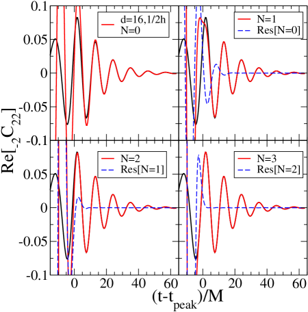
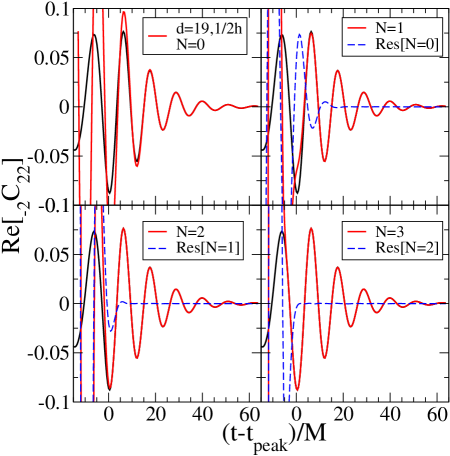
Figure 15: Comparison of numerical and QNM ${}_{-\!2}C_{22}$ ring-down waveforms for $d=16$ and $19$. All plots show the numerical ring-down waveform as a thin solid (black) line. The thick solid (red) line displays the fit of the ring-down signal using the first $N$ $\ell=2,m=2$ overtones beyond the fundamental. For plots containing $N>0$ overtones, we also include the fit residual from the previous value of $N$. This is displayed as a dashed (blue) line. The coefficients for the displayed fits are found in Tables 8 and 9.

A close examination of Tables 7–9 reveals a significant level of consistency to the fits. For each separation $d$, the spin and mass ratios remain very consistent and the ${\cal C}_{22n}$ and $\phi_{22n}$ coefficients remain quite consistent, as we increase the number of overtones included in the fits. This is true individually within the separate fits of the real and imaginary parts of ${}_{-\!2}C_{22}$, and consistency is also seen between the fits of the real and imaginary parts. While the $\ell=2$, $m=2$ QNMs seem to dominate the ring down signal in ${}_{-\!2}C_{22}$, the $\ell=2$, $m=-2$ modes and the modes with $\ell>2$ should be present. However, the remaining residual after the $N=3$ fit (not shown in any figure) has very low amplitude at times after the peak in $|{}_{-\!2}C_{22}|$. While there are some hints to structure, there is insufficient signal and the simple approach we have used for fitting does not yield consistent fits when additional modes are included.

However, if we fix the values for $a/M_{f}$ and $M_{f}/M$ to the values obtained from the $\ell=2$, $m=2$ fits, we can fit for the ${\cal C}_{\ell\pm\!2n}$ and $\phi_{\ell\pm\!2n}$ coefficients for a range of modes. Doing so, we find that the fundamental QNM with $\ell=3$, $m=-2$ has the most significant contribution, followed by the $\ell=4$, $m=-2$ and $\ell=3$, $m=2$ fundamental modes at roughly comparable levels. Unlike the case of fitting only the $\ell=2$, $m=2$ modes, adding in higher overtones when an increased spectrum of modes was considered did not lead to consistent fits. Part of the difficulty in finding consistent fits to the subdominant modes is likely due to the fact that the signal associated with these modes is close to the level of numerical precision in the waveform. However, it is also likely that more sophisticated fitting methods are needed. In particular, it would be useful to fit the real and imaginary parts of the waveform simultaneously. It may also be helpful to fit several ${}_{-\!2}C_{\ell m}$ modes simultaneously.

While fitting multiple modes is problematic in some cases, it is essential in others. For the case of ${}_{-\!2}C_{32}(t)$, the dominant QNMs include both $\ell=2$ and $\ell=3$, both with $m=2$. In fact, it was not possible to fit the ring-down signal of ${}_{-\!2}C_{32}(t)$ without fitting simultaneously for these two modes. To be explicit, we take as our fitting function:

$${}_{-\!2}C_{32} = \sum_{n=0}^{N}\bigl{\{}{\cal C}_{322n}e^{-i(\hat{\omega}_{22n}(a/M_{f},M_{f}/M)(t-t_{\rm peak})+\phi_{322n})}$$

$$\mbox{}\hskip 18.06749pt+{\cal C}_{332n}e^{-i(\hat{\omega}_{32n}(a/M_{f},M_{f}/M)(t-t_{\rm peak})+\phi_{332n})}\bigr{\}}.$$

Fitting proceeds as with ${}_{-\!2}C_{22}$, starting with $N=0$ and then adding successive overtones which allow us to fit to successively earlier times in the ring down.

Tables 10, 11, and 12 in Appendix D display the fit parameters for the ${}_{-\!2}C_{32}(t)$ waveform obtained from initial data with separation parameter $d=13$, $d=16$ and $d=19$. Figure 16 shows the quality of the fit to ${\rm Re}[{}_{-\!2}C_{32}(t)]$ for the cases $N=0,1,2$ and for the separations $d=16$ and $19$. We note that by including modes through the $n=2$ overtone, we can again fit the ring down quite well to times preceding the point where $|{}_{-\!2}C_{22}|$ reaches its peak. As for ${\rm Re}[{}_{-\!2}C_{22}(t)]$, we also include the residuals of the previous fit. We note that the level of consistency of the fits, though significant, is not as high for ${}_{-\!2}C_{32}$ as seen for ${}_{-\!2}C_{22}$.

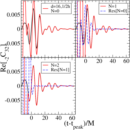
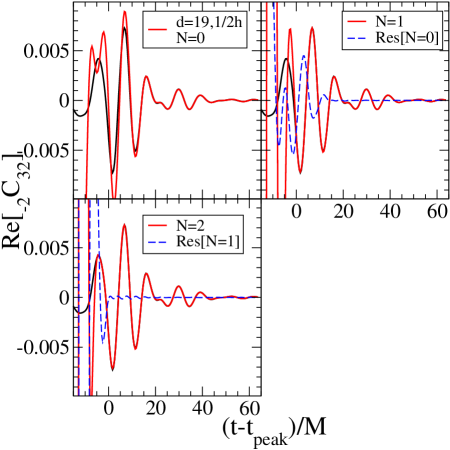
Figure 16: Comparison of numerical and QNM ${}_{-\!2}C_{32}$ ring-down waveforms for $d=16$ and $19$. All plots show the numerical ring-down waveform as a thin solid (black) line. The thick solid (red) line displays the fit of the ring-down signal using the first $N$ $\ell=2,m=2$ and $\ell=3,m=2$ overtones beyond the fundamental. For plots containing $N>0$ overtones, we also include the fit residual from the previoius value of $N$. This is displayed as a dashed (blue) line. The coefficients for the displayed fits are found in Tables 11 and 12

During the ring-down phase, it is possible for a few percent of the final mass $M_{f}$ and angular momentum $aM_{f}$ to be radiated away from the system. The Kerr QNM frequencies and decay constants are computed assuming that the mass and angular momentum they carry away constitute a negligible perturbation on the system. This raises the question as to whether or not the radiated energy and angular momentum are affecting the QNM fits. This issue will, of course, become more significant as the fits are pushed to earlier times. As we have seen for the cases of ${}_{-\!2}C_{22}$ and ${}_{-\!2}C_{32}$, fitting to earlier times in the ring down requires the use of higher overtones ($n>0$) with shorter decay times. Because these higher overtones dominate the waveform only at earlier times in the ring down, we should expect some increase in the level of uncertainty in the fits as we incorporate these overtones.

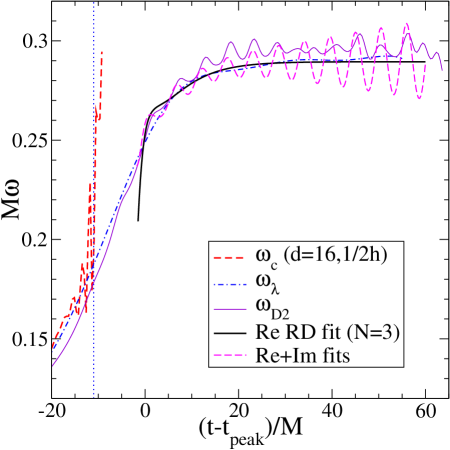
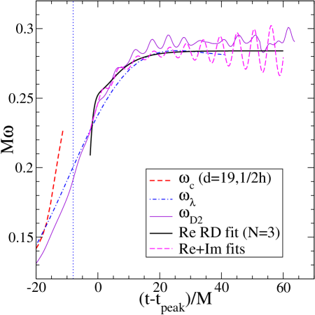
Figure 17: Dominant frequencies during the ring down for the $d=16$ and $19$ cases evaluated using several methods. The short dashed (red) line is $\omega_{c}$. The dot-dashed (blue) line is $\omega_{\lambda}$. And the thin solid (purple) line is $\omega_{\rm D2}$. These three lines were previously displayed in Fig. 7. The thick solid (black) line shows the dominant frequency of Eq. (43) as fit to the real part of the ${}_{-\!2}C_{22}$ ring-down signal. The long-dashed (magenta) line shows the dominant frequency of a similar fit, but consistently using the both the real and imaginary fits to ${}_{-\!2}C_{22}$. The vertical dotted (blue) line marks the approximate time that a common AH forms.

Finally we want to revisit the plots of the orbital angular frequency displayed in Fig. 7. The $\omega_{\lambda}$ and $\omega_{D2}$ frequencies continue beyond the inspiral phase and through the ring down. Beyond the inspiral phase, this frequency clearly cannot be associated with the orbital angular frequency. Rather they are half of the dominant GW frequencies seen in ${}_{-\!2}C_{22}$. In Fig. 17, we plot this dominant frequency from a time about $10M$ before the formation of a common AH and through the ring down. In this range of times, $\omega_{c}$ clearly decouples from $\omega_{\lambda}$ and $\omega_{\rm D2}$. As the dynamics transitions from the inspiral phase, the dominant frequency rises very rapidly, finally reaching a plateau associated with the dominant QNM ring-down frequency. Both $\omega_{\lambda}$ and $\omega_{\rm D2}$ agree quite well through both the transition and ring down, but we note that $\omega_{D2}$ shows an unusual “beating” of the frequency during the ring down.

We also plot in Fig. 17 the dominant frequency as measured by the fits to the ring down. Using the ring-down fit function in Eq. (43) together with the fit value given in Tables 7–9 yields an analytic expression for ${}_{-\!2}C_{22}$ through the ring-down phase. Because we independently fit Eq. (43) to the real and imaginary parts of ${}_{-\!2}C_{22}(t)$ we have three different ways that we can construct ${}_{-\!2}C_{22}$. We can take the coefficients for the fit from either ${\rm Re}[{}_{-\!2}C_{22}]$ or ${\rm Im}[{}_{-\!2}C_{22}]$ and use that set of coefficients exclusively in Eq. (43). Using the analytic representation of ${}_{-\!2}C_{22}(t)$ we can compute the dominant frequency using Eq. (23) with $m=2$. A plot of this frequency using the coefficient obtained form the fit of ${\rm Re}[{}_{-\!2}C_{22}]$ is shown if Fig. 17 with the label “Re RD fit (N=3).” Notice that the frequencies agree well during the ring-down phase and show a period following the peak in $|{}_{-\!2}C_{22}|$ where the frequency increases before reaching its plateau. Also, we see no evidence of the beating seen in $\omega_{\rm D2}$.

However, if we instead construct an analytic representation of ${}_{-\!2}C_{22}$ using the coefficients from the fits to both ${\rm Re}[{}_{-\!2}C_{22}]$ and ${\rm Im}[{}_{-\!2}C_{22}]$, we recover the beating of the frequency. To be clear, using Eq. (23) to construct the dominant frequency incorporates both the real and imaginary parts of ${}_{-\!2}C_{22}$. If we consistently use the coefficients from the fit to ${\rm Re}[{}_{-\!2}C_{22}]$ when constructing an analytic representation for ${\rm Re}[{}_{-\!2}C_{22}]$ and use the coefficients from ${\rm Im}[{}_{-\!2}C_{22}]$ for its representation, then we obtain the line labeled “Re+Im fits” in Fig. 17. The plot of this frequency clearly shows a beating of the frequency and this is due to a small mismatch between the real and imaginary fit coefficients. It seems clear that the beating we observe in $\omega_{\rm D2}$ is caused by a similar effect. Essentially, numerical error is leading to a non-physical mode that is not circularly polarized, leading to the mismatch seen between the real and imaginary parts of $\Psi_{4}$.

VI The (plunge and) merger

In Sec. III.4 we discussed the possible presence of a rather blurred dynamical ISCO which marks the beginning of the plunge phase. The latter ends when the CAH forms. The plunge has a duration of $30\mbox{--}50M$, corresponding to $1\mbox{--}1.5$ GW cycles. The plunge cycle has a slightly different shape than the inspiralling cycles when viewed in ${\rm Re}[{}_{-\!2}C_{22}]$ (see Fig. 11), but it can barely be distinguished from the inspiralling cycles when viewed in $h_{+}$ and $h_{\times}$ (see Fig. 12). Quite interestingly we notice that the onset of the plunge phase seems to happen soon after the “knee” in the frequency curve (see Fig. 7), and when the first change in the slope of the GW energy flux occurs (see Fig. 26, especially the right panel). A second change of slope in the frequency and GW energy flux seems to happen roughly around the CAH, the third change occurs at the peak of the radiation.

In Fig. 18 we illustrate some other interesting features of the inspiral to ring-down transition, i.e., the binary BH merger. We plot the frequencies $\omega_{c}$ and $\omega_{\lambda}$, and the GW energy flux (multiplied by 100). Circles mark the position (time and frequency) at which the CAH forms and show when the coordinate separation between the BHs become less that the estimated co-rotating light ring of the final BH. The latter are coordinate dependent quantities. The light ring is an unstable circular null geodesic of the Kerr geometry in the equatorial plane of the BH, and we estimate the position of the light ring by noting that for a Kerr BH with $a=0.70$, in Boyer-Lindquist coordinates the co-rotating light ring is a radial distance of $\approx 1.17$ times that of the outer horizon BM . For an estimate of the light-ring location in the generalized harmonic coordinates of the simulation we took the late-time coordinate radius of the final AH multiplied by $1.17$. Of course the different coordinates used to arrive at this value make it a rather rough estimate, though given that the notion of a light ring is not well-defined near coalescence it would not add much if we found the exact location. When the equal-mass binary reaches the CAH, only half of the total energy has been released. A little while before this point we observe that $\omega_{\lambda}$ decouples from $\omega_{c}$. Note also that at the peak of the radiation, $23\%$ of the total energy has yet to be released. Here and in the following, the total energy refers to the energy radiated from the beginning of the simulation until the end. Thus, it doesn’t include the energy radiated during the long inspiral preceding the initial time of the simulation.

The results obtained in Sec. V, in particular Figs. 17 and discussion around them, suggests that the GW emission soon after the peak of radiation is caused by the excitation of the QNMs of the final Kerr BH. The frequency of the least damped QNM $l=2,m=2,n=0$ is responsible for the plateau, and the higher overtones ($l=2,m=2,n>0$), which have smaller frequencies and smaller decay times, should be responsible for raising the frequency from the peak of the radiation to the plateau. It is still not completely clear to us whether the higher overtones and/or other QNMs, e.g., $l=2,m\neq 2,n\geq 0$, are able to smoothly connect the decoupling frequency with the plateau. In fact, soon after the decoupling, there could be a very short non-linear phase, perhaps with strong mode mixing, that would preclude a description in terms of QNMs. To clarify those issues, it would be interesting to compute the binary BH metric around the decoupling point or the CAH, decompose it as a single Kerr metric plus perturbations, e.g., as done in the close limit approximation PP94 ; AC ; GNPP ; Pullin99 , and determine more precisely when the perturbative regime starts. In the next section, following a more phenomenological approach aimed at providing templates for GW detection, we will see how the ring-down phase could be matched to the inspiral phase in the EOB model, assuming that the QNMs are responsible for raising the frequency from the decoupling to the plateau.

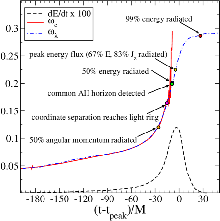
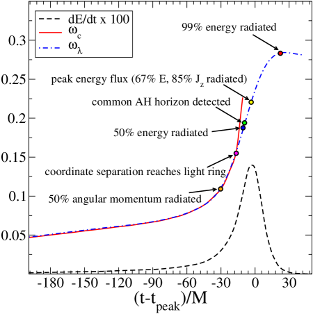
Figure 18: Features of the merger phase. We plot the frequency evaluated from the orbit and the wave, and the GW energy flux. We mark with circles the time when the common AH of the final BH first appears, when the binary separation reaches the light-ring of the final BH, the peak of the radiation flux (which occurs around $3-4M$ before the peak in the amplitude of the waveform), when $50\%$ of the energy and angular momentum have been radiated, and the time when $99\%$ of the energy has been radiated ($99\%$ of the angular momentum appears to be radiated around $5-10M$ before this, though due to the oscillations in $dJ_{z}/dt$ we are much less certain exactly when this occurs—see Fig.27). The left panel refers to the $d=16$ run and the right panel to the $d=19$ run.

Finally, if we denote by merger the phase from roughly the decoupling point when $M\,\omega_{\rm dec}\sim 0.14\mbox{--}0.16$ to the peak of ${\rm Re}[{}_{-\!2}C_{22}]$ when $M\,\omega_{\rm peak}\sim 0.2$ or the peak of radiation, the merger occurs in a very short time $\approx 10\mbox{--}15M$, corresponding to $\approx 0.5\mbox{--}0.75$ GW cycles. During this phase the frequency increases by $\approx 45\%$, causing the GW spectrum to spread over a large frequency range (see Figs. 22 and 23). We shall discuss how this will affect the detectability of GWs from equal-mass binaries in Sec. VIII.

VII Effective-one-body approach to inspiral–(plunge)–merger–ring-down

The Taylor-expanded Hamiltonian for a two-body system was computed at 3PN order in Refs. DJSdr ; JS . It took several years to compute the GW energy flux at 3.5PN order 35PNnospin . Before the 3.5PN dynamics was completed the Taylor-expanded PN predictions for the GW energy flux and the phasing of equal-mass binaries were not accurate enough to obtain robust predictions of the GW signal during the last stages of inspiral and plunge. For example, through 2.5PN order, the PN-approximants of some of the crucial ingredients entering the GW signal, such as the GW energy flux, differ significantly when evaluated at subsequent PN orders in the typical frequency band of ground-based detectors DIS98 . On the other hand, the signal-to-noise ratio of ground-based interferometers (especially the LIGOs) reaches its maximum around comparable-mass binaries. Thus, likely, the first detection may come from a coalescence of stellar–comparable-mass BHs merging in the most sensitive region of the detector’s frequency band.

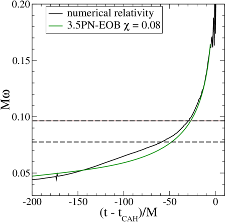
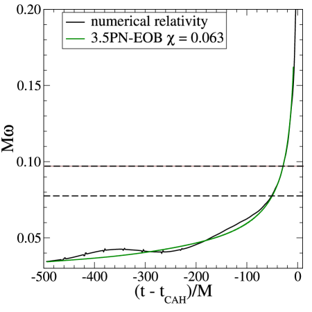
Figure 19: We compare the NR orbital frequency and the EOB orbital frequency obtained using the nominal $\chi$ value from Table 1. The left panel refers to the run $d=16$, the right panel to $d=19$. The horizontal light continuous line marks the ISCO frequency, as predicted by the conservative 3PN-EOB Hamiltonian. The two dashed lines span the region in which a dynamical ISCO might be present.

At the beginning of 2000, in absence of NR results and under the urgency of providing templates to search for comparable-mass BHs, some resummation techniques of the PN series were proposed. In Ref. DIS98 , the authors proposed the Padé resummation of the two-body energy and the GW energy flux, and in Refs. BD1 a specific resummation of the PN Hamiltonian was proposed, the so-called effective-one-body (EOB) Hamiltonian. Later on, in Ref. BD2 the last stages of inspiral and plunge were modeled by combining the EOB Hamiltonian with the Padé resummation of radiation-reaction effects, providing the GW signal which includes effects beyond the adiabatic approximation. The EOB Hamiltonian was then extended at 3PN order without spin effects in Ref. DJS and with spin effects in Ref. TD . More recently, the transition from inspiral to plunge including spin couplings has been modeled in Ref. BCD . These analytical studies predicted that (i) the two-body motion would be quasi-circular throughout the last stages of inspiral and plunge, until the light-ring (see Fig. 1 in Ref. BD2 ), (ii) the ISCO for an equal-mass binary is a rather blurred concept, taking place roughly during half of a GW cycle (see Fig. 12 in Ref. BD2 ) and that (iii) the adiabatic plunge lasts only for almost one GW cycle (see Fig. 12 in Ref. BD2 ).

In Refs. BD2 ; BCD , the authors also provided an example of the full waveform by modeling the merger as a very short (instantaneous) phase and by matching the natural end of the EOB plunge (around the light-ring) with the ring-down phase (see Ref. lazarus where similar ideas subsequently developed also in NR). The matching was done using only the least damped QNM whose mass and spin were determined by the binary BH energy and angular momentum at the end of the EOB plunge. The choice of the light-ring at $\approx 3M$ for shifting the description between a (quasi-circular) binary motion and a deformed Kerr BH, was inspired by two considerations BD2 . First, in the test-mass limit, $\nu\ll 1$, Refs. Davis ; Press (see also Ref. BM ) realized a long time ago that the basic physical reason underlying the presence of a universal merger signal was that when a test particle falls below $3M$ (which is also the unstable light storage ring of Schwarzschild), the GW it generates is strongly filtered by the effective potential barrier centered around it. Secondly, for the equal-mass case $\nu=1/4$, the close limit approximation PP94 ; AC ; GNPP ; Pullin99 ; AHSSS suggests a matching between the two-body and the perturbed-black-hole descriptions when the distance modulus $\mu_{0}\simeq 2$, which would correspond to a Schwarzschild-like radial distance $\simeq 2.6M$.

For non-spinning, equal-mass binaries, the EOB approach predicts at 3PN order BCD : $a_{\rm end}/M_{\rm end}\simeq 0.77$, $M_{\rm end}\simeq 0.974\,M$, an energy released of $\simeq 1.3\%M$ until $t_{\rm end}$ and $\approx 1\%$ from the least-damped QNM phase BD3 ; BCD . Here and henceforth we denote by the subscript “${\rm end}$” the time at the end of the EOB plunge. Depending on the PN order the ending time can occur slightly before the conservative light-ring. $t_{\rm end}$ is the time at which the quasi-circular assumption used in building the EOB equations of motion breaks down BCD .

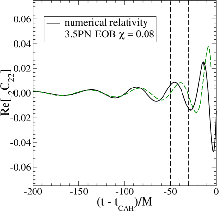
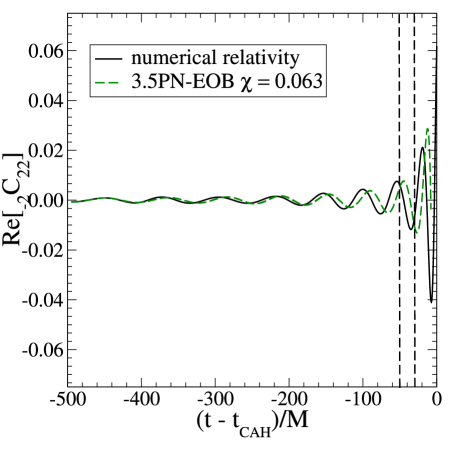
Figure 20: We compare the NR ${\rm Re}[{{}_{-2}C_{22}}]$ and the EOB ${\rm Re}[{{}_{-2}C_{22}}]$ waveforms obtained using the nominal $\chi$ value from Table 1. The left panel refers to the run $d=16$, the right panel to $d=19$. The two vertical dashed lines span the region in which a dynamical ISCO might be present.

We show now some first-order comparisons between the numerical waveforms and the EOB waveforms, evaluated with the EOB conservative dynamics at 3PN order with spin-orbit and spin-spin effects included through 2PN order, and Padé radiation-reaction energy flux at 3.5PN order BCD . In contrast to the PN adiabatic model discussed in Sec. IV.2, which should be used with confidence only until the last stable orbit, the EOB model extends beyond it through the plunge.

In Sec. IV.2 a comparison of the PN orbital frequency with the numerical results was obtained by fitting to the orbital frequency $\omega_{c}$. In the EOB model the orbital frequency is obtained by solving the EOB equations of motion, thus it is more complicated to implement a least-square fit. Here, we simply determine by hand which initial EOB orbital frequency best matches, on average, the numerical orbital frequency $\omega_{c}$ from the initial time to the light-ring or CAH (see Sec. VI), and compute the corresponding wave. In Fig. 19 we show the results for the $d=16$ and $d=19$ runs assuming the nominal $\chi$ value from Table 1. At the initial time $t=0$, we find $M\,\omega_{0}=0.047$, $E_{0}/M=0.986$, $J_{0}/M^{2}=0.896$ for $d=16$ and $M\,\omega_{0}=0.034$, $E_{0}/M=0.988$, $J_{0}/M^{2}=0.945$ for $d=19$. The evolution ends at $r_{\rm end}\simeq 2.5\,M$, where $M\,\omega_{\rm end}\simeq 0.16$, $E_{\rm end}/M\simeq 0.971$, $J_{\rm end}/M^{2}\simeq 0.741$ for the $d=16$ run, and at $r_{\rm end}\simeq 2.5\,M$ where $M\,\omega_{\rm end}\simeq 0.16$, $E_{\rm end}/M\simeq 0.971$, $J_{\rm end}/M^{2}\simeq 0.737$ for the $d=19$ run. We notice that the EOB conservative ISCO for $\chi=0.063$ is at $M\,\omega_{\rm ISCO}\sim 0.096$ TD ; BCD , rather close to the frequency range $M\omega_{\rm dyn\,ISCO}=0.078\mbox{--}0.097$ of the dynamical ISCO discussed in Sec. III.4. In Fig. 20 we compare the NR and EOB ${\rm Re}[{{}_{-2}C_{22}}]$ waveforms. The two vertical dashed lines in Fig. 20 mark the region during which a dynamical ISCO may be present. We compute the EOB waveform using Eq. (26), which is valid in the adiabatic circular-orbit case. We checked that by relaxing this assumption and computing ${\rm Re}[{{}_{-2}C_{22}}]$ by taking derivatives of the binary quadrupole moment, the wave does not change much, except at the very end.

By assuming the merger is a very short phase, the authors of Ref. BD2 simply joined the GW signal at the end of the inspiral to the least-damped QNM. As said above this modeling was inspired by the idea that once beyond the light-ring (i.e., inside the potential barrier), the GW emission is quickly dominated by the excitation of the QNM of the newly-formed BH. The choice of matching only one QNM inevitably creates a sudden jump of the GW frequency at the matching point. However, a smoother transition can be obtained by including higher overtones. As discussed in Sec. VI, the analysis done in Sec. V would suggest that the QNM production starts a bit later, around the peak of the radiation. At this stage we do not know whether a linear superposition of QNM can be responsible for raising the frequency from around the light ring (see Fig. 18) to the peak of radiation. In the spirit of an effective approach aimed at modeling the GW signal for detection, we push this idea further by including higher overtones when matching to the ring-down phase and discuss the consequences. The inclusion of higher overtones when matching to the ring-downn phase has also recently been adopted in Ref. DNT , where the authors computed the transition inspiral–plunge–ring-down of a test particle in Schwarzschild. By including higher overtones, the authors could successfully match the exact numerical rise of frequency from the light ring to the least damped QNM as obtained from the Zerilli equation.

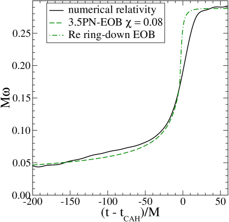
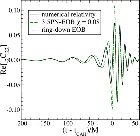
Figure 21: We compare the NR and EOB frequency and ${\rm Re}[{{}_{-2}C_{22}}]$ waveforms throughout the entire inspiral–merger–ring-down evolution. The data refers to the $d=16$ run.

First, we evaluate the BH mass and angular-momentum at the end of the EOB plunge, finding $M_{\rm end}\equiv E_{\rm end}\simeq 0.971\,M$ and $a_{\rm end}/M_{\rm end}\equiv J_{\rm end}/E^{2}_{\rm end}\simeq 0.785$. Then, we notice that those values are not the final BH mass and angular momentum because the binary has yet to emit energy and angular-momentum from the light-ring or CAH to the least-damped mode (see discussions around Fig. 18). Future NR simulations will provide predictions for different mass ratios and spins. Here, guided by the results of Sec. VI and Fig. 18, we assume that $(M_{\rm end}-M_{f})/M_{\rm end}=1.5\%$ and $(a_{\rm end}-a_{f})/a_{\rm end}=6\%$. Thus, we obtain $M_{f}=0.956\,M$ and $a_{f}/M_{f}=0.738$. Using Ref. BCW , we determine the frequency and the decay time of the fundamental mode and the first two overtones, finding $M\,\omega_{220}=0.576$, $M\,\omega_{221}=0.565$, $M\,\omega_{222}=0.545$, $\tau_{220}/M=0.0828$, $\tau_{221}/M=0.250$ and $\tau_{222}/M=0.422$. We then determine the three unknown amplitudes and three unknown phases of the three QNMs by imposing the continuity of the frequency $\omega_{\rm D2}$, Eq. (23), the wave and its first five derivatives at $t=t_{\rm end}$. We note that this matching procedure is rather sensitive to the time of matching because the frequency is increasing very quickly around $t_{\rm end}$. In Fig. 21 we compare the frequency and the inspiral–(plunge)–merger–ring-down wave ${\rm Re}[{{}_{-2}C_{22}}]$ of the EOB model with the NR results for the case $d=16$. The EOB ring-down frequency is computed from Eq. (23) where we used in ${\rm Im}[{{}_{-2}C_{22}}]$ the same three amplitudes and three phases of ${\rm Re}[{{}_{-2}C_{22}}]$. Were we to use in ${\rm Im}[{{}_{-2}C_{22}}]$ the three amplitudes and phases obtained by matching it at $t_{\rm end}$, we would not obtain a good result. This is due to numerical errors introduced by matching separately ${\rm Re}[{{}_{-2}C_{22}}]$ and ${\rm Im}[{{}_{-2}C_{22}}]$ at $t_{\rm end}$.

As seen in Fig. 21, by matching the fundamental QNM and the first two overtones, the frequency transition becomes smoother, but nevertheless it differs from the NR frequency $\omega_{\lambda}$. As we shall see in the next section, this effective way of including a short in time, but spread in frequency, merger phase, can mimic the frequency spread of the power spectrum of the NR waves, though with a slightly different power law.

VIII Detectability of the signal

In this section we compute the Fourier transform of the numerical waveforms, compare the results with the analytical predictions and give an estimate of the optimal signal-to-noise ratio (SNR) for ground-based and space-based detectors.

Frequency domain PN templates for the inspiral phase are generally computed in the so-called Stationary Phase Approximation (SPA). They read

$$h_{\rm SPA}(f)={\cal A}\,f^{-7/6}\,e^{i\Psi_{\rm SPA}(f)}\,,\quad\quad{\cal A}=\frac{1}{\sqrt{30}\pi^{2/3}}\frac{{\cal M}_{c}^{5/6}}{D_{\rm L}}\,$$ (45)

where $f$ is the frequency of the GWs, ${\cal M}_{c}=\nu^{3/5}M$ is the chirp mass and $D_{\rm L}$ is the luminosity distance to the source. In Eq. (45) we have adopted the standard “restricted PN approximation”, in which the amplitude is expressed to the leading order in a PN expansion while the phasing $\Psi_{\rm SPA}(f)$, is expressed to the highest PN order available. The phase is currently known through 3.5PN order. Here, we are only interested in computing the amplitude of the Fourier transform of the signal and investigating how and when it starts deviating from the Newtonian prediction $f^{-7/6}$. We shall analyze the comparisons between the Fourier transform phases in the future.

In the left panel of Fig. 22 we plot the Fourier transform amplitudes of the numerical waveform for the three runs, for a $(15+15)M_{\odot}$ binary which is a typical source for LIGO/VIRGO/GEO/TAMA. Using Table I we find that for this binary mass the initial GW frequency in the three runs is $121$ Hz, $89$ Hz and $71$ Hz (vertical dot lines in the left panel of Fig. 22) . To compute the Fourier transform we extrapolate the numerical waveforms at earlier time, for almost $6\times 10^{4}$ m, by attaching to it the 3PN-adiabatic model which best-fits it. We compute the Fourier transform in three different ways, from ${\rm Re}[\Psi_{4}]$ and $h_{+}$ extracted along the direction perpendicular to the orbital plane, and from ${{}_{-2}C_{22}}$. Besides a normalization factor, the amplitudes computed from ${\rm Re}[\Psi_{4}]$ and ${{}_{-2}C_{22}}$ must agree in the inspiral phase, where they satisfy more and more the restricted PN approximation, but they can differ in the last part of inspiral, merger and ring-down, when non-linear effects and higher harmonics can become important.

From Fig. 22, we see that at low-frequency, during the last stages of inspiral, the amplitude can be approximated by the Newtonian amplitude $f^{-7/6}$, with small bumps maybe due to the presence of eccentricity. At higher frequency, during the merger and ring-down the slope changes to $f^{-n}$. At this stage we cannot uniquely determine the slope index or say if there is more than one change in the slope. We estimate $n\approx 0.6\mbox{--}0.8$  and notice that the change in the slope can occur as early as the beginning of the plunge $M\omega\sim 0.1$ or as late as the decoupling time $M\,\omega\sim 0.16$. As an example in Fig. 22 we show the case $n=2/3$. Finally, the signal drops at higher frequencies, around the frequency of the fundamental QNM, i.e., $620$ Hz for the $(15+15)M_{\odot}$. Even if the merger occurs in a short time, corresponding to $\approx 0.5\mbox{--}0.75$ GW cycle, the frequency increases very quickly during this phase and then approaches the frequency of the fundamental QNM. As a consequence, the Fourier transform signal spreads over a large frequency band $300\mbox{--}600$ Hz. We also computed the Fourier transform amplitude from $\Psi_{4}$ extracted along directions $\theta\neq 0$, and found differences in the merger–ring-down amplitude slope. We shall discuss those interesting features in a future publication.

In the right panel of Fig. 22, we show the sky averaged SNRs versus total mass, for an equal mass binary at 100 Mpc, and for initial LIGO. The dashed-dot and dashed curves are computed assuming the SPA inspiral signal (45) until the Schwarzschild ISCO $f_{\rm ISCO}=4400/(M/M_{\odot})$ and the ICO predicted by adiabatic PN theory at 3PN order ICO , respectively. The average SNR for one detector for an SPA signal is computed using

$$\sqrt{<{\rm SNR}^{2}>}=\frac{1}{D_{L}}\,\frac{1}{\pi^{2/3}}\,\sqrt{\frac{2}{15}}\,{\cal M}_{c}^{5/6}\,\left[\int_{f_{\rm low}}^{f_{\rm high}}\frac{f^{-7/3}}{S_{n}(f)}\right]^{1/2}\,.$$ (46)

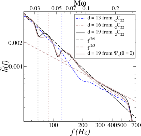
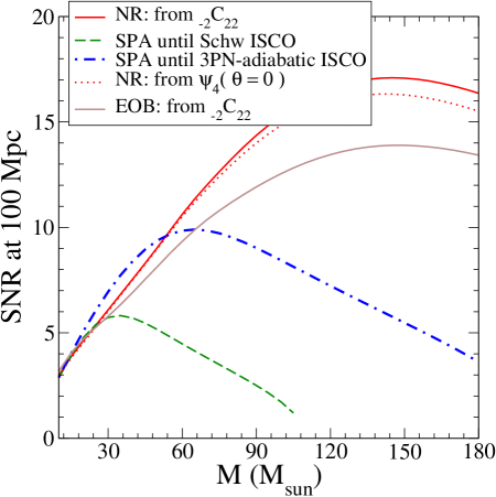
Figure 22: In the left panel we plot the amplitude of the Fourier transform of the numerical waveform for a binary with (redshift) mass $(15+15)M_{\odot}$. The lower horizontal axis marks the gravitational wave frequency in Hz, while the upper axis marks the dimensionless orbital angular velocity that coincides with the instantaneous GW frequency. The vertical dotted lines mark the frequencies at which the runs start. In the right panel, we show the average SNR for one detector versus the (redshift) total mass for an equal-mass binary at 100 Mpc.

The continuous light curve in Fig. 22 is computed from the EOB inspiral–(plunge)–merger–ring-down wave shown in Fig. 21. The change in the slope that we observe in the left panel of Fig. 22, together with the inclusion of the signal beyond the ISCO, causes an increase of the SNR for large masses BD2 ; TD ; BCD ; FH . For total masses lower than $(15+15)M_{\odot}$, the end of the inspiral occurs around the most sensitive LIGO frequency, while the merger–ring-down is pushed to higher frequency where the sensitivity is much lower. As a consequence, the average SNR which includes merger and ring-down phases does not differ much from the one that includes only the inspiral phase. Astrophysical observations and theoretical predictions suggest that stellar mass BHs have a total mass ranging between $6\mbox{--}30M_{\odot}$. If binary BHs of larger total mass exist, they could be detected by initial LIGO with very high SNR. The EOB model with the instantaneous matching to three QNMs predicts a SNR close to the NR result. It is smaller because the effective matching of the inspiral to the three QNMs (see Fig. 21) gives a Fourier transform amplitude which extends until the QNM frequency, but with a slope index slightly larger than $\approx-0.6\mbox{--}0.8$.

In the left panel of Fig. 23 we plot the amplitude of the Fourier transform for a signal typical of LISA, a $(10^{6}+10^{6})M_{\odot}$ supermassive BH binary. In the right panel we show the average SNR for one Michelson LISA configuration versus the total (redshift) mass for an equal-mass binary at 3 Gpc. The dip in the plot is due to the WD-WD confusion noise BBW . Due to the inclusion of merger and ring-down phases, the SNR increases considerably for total masses larger than $2\times 10^{6}M_{\odot}$. We notice that Fig. 23 is consistent with Fig. 7 of Ref. BCW where the authors computed the SNR due to the ring-down phase, assuming $\sim 3\%m$ of energy released during the merger.

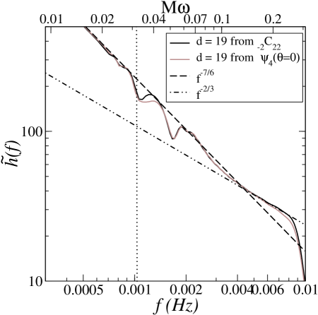
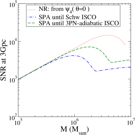
Figure 23: In the left panel we plot the amplitude of the Fourier transform of the numerical waveform for a binary with (redshift) mass $(10^{6}+10^{6})M_{\odot}$. The lower horizontal axis marks the gravitational wave frequency in Hz, while the upper axis marks the dimensionless orbital angular velocity that coincides with the instantaneous GW frequency. The vertical dotted line marks the frequency at which the $d=19$ run starts. In the right panel we show the average SNR versus the (redshift) total mass for an equal-mass binary at 3 Gpc ($z=0.54$).

IX Conclusions

In this paper we have analyzed the data of several numerical simulations of the inspiral–merger–ring-down of an equal-mass binary carrying a very small spin aligned with the orbital angular momentum.

The combination of several effects including (i) limited resolution, (ii) relatively close initial configurations and (iii) lack of diagnostics to measure and compensate for possible coordinate artifacts, make it impossible to claim very high accuracy in the comparisons with analytical models and the analysis of the merger waveform. Nevertheless, the resolution studies performed in Sec. III suggest that we are in the convergent regime, and so meaningful conclusions can be drawn from the data. Furthermore, the consistency with which several quantities have been measured by independent means suggest that adverse gauge effects are minor and will not affect many of the conclusions reached. In particular, as Tables 3 and 5 show, the final mass and angular momentum extracted from the ring-down are very close to their values measured through AH properties. Also, the orbital frequency measured via AH motion is close to the one extracted from the GW, as Fig. 7 shows.

We found that one of the dominant forms of numerical error is a slow drift in the phase of the waveform. With respect to detectability in a GW burst-search this error does not seem to be very significant, as the cumulated phase error up to the peak in the radiation can be factored out by a constant phase shift and the subsequent coalescence/ring-down waveform does not seem to be significantly affected by prior phase error. However, for matching to PN models at earlier time and parameter estimation this error is significant, and directly translates into uncertainties in matching parameters.

As Figs. 2 and 3 show, the numerical evolution is characterized by a strong initial pulse of radiation. The timing of the pulse suggests that it is associated with the assumption of conformal flatness. In fact it has very similar characteristics to the initial pulse seen in scalar field collapse generated binaries FP ; FP3 , which also begin with a conformally flat spatial metric. Fortunately, the effects of this pulse of radiation seem to diminish rapidly. The initial data does not put the binary on a clean circular inspiral path. As discussed in Sec. III.4 (see Fig. 5), the trajectory clearly oscillates about the desired trajectory. The effects of this oscillation can be interpreted as a small eccentricity of the initial orbit. We estimated it to be $e\sim 0.02$ for the $d=19$ case. While these oscillations could be due to an actual eccentricity in the initial data, they could also be due to a lack of an appropriate initial radial momentum. The current simulations cannot determine which effect, if either, is most significant. However, while there are oscillations in the inspiral trajectory, the resulting dynamics is still adiabatic (e.g., see Fig. 6) and modeled well by circular orbits.

Concerning the inspiral phase, as described in Sec. IV.1 it is remarkable how well the Newtonian quasi-circular approximation can match the numerical signal of an equal-mass binary. For this we mean that if the orbital phase is modeled well, the leading order Newtonian term in the expansion of the waveform is able to model both the amplitude and phase of the GW quite accurately until close to the time of merger. It is also striking how, despite possible coordinate artifacts, a GW signal computed with the leading quadrupole formula using the coordinate motion of the AH’s matches the numerically extracted wave to a reasonable degree (see Fig. 9).

As discussed in Sec. IV.2, the PN adiabatic phase and frequency matches $\omega_{c}$ (frequency computed from the AH motion) well. In particular, if the analytical expressions for $\omega$ (28) and $\phi$ (31) are used, the 3PN-approximant best fits the data, whereas if the expression for $\dot{\omega}$ (32) is solved numerically, a 3.5PN-approximant also matchs the numerical data to a similar level. The accuracy of the PN-adiabatic model improves with increasing binary separation. We expect it deviates from non-adiabatic models when approaching the last stable orbit. Nevertheless, we found that if the PN-adiabatic model is extrapolated even to the formation of the CAH, it gives reasonable results. This is due to the fact that the numerical plunge cycle is very short and still quasi-circular for an equal-mass binary, as originally predicted in the EOB model BD2 . In Sec. VII we compared the numerical results with the EOB model. Again we found that the 3.5PN-approximant best matches the data. The blurred ISCO phase of half of a GW cycle and subsequent plunge phase of almost one GW cycle predicted in the EOB model BD2 seems to be consistent with the numerical results. By properly adjusting the mass and angular-momentum of the BH at the end of the EOB plunge, to account for the energy and angular-momentum released during the merger, and by including three QNMs, we could match the EOB inspiral-(plunge) wave to the ring-down wave (see Fig. 21). This matching procedure is very sensitive to the time of matching and it is only partially effective (see the difference in the GW frequency in Fig. 21) since it does not capture the details of the merger, but could be improved in the future.

As Fig. 7 shows, $\omega_{c}$ decouples from the dominant GW frequency just before the point of formation of the common AH, around the light ring. We conjecture that this decoupling time marks the transition point between inspiral-(plunge) and merger. We found that the merger accounts for only a brief time ($\sim 10\mbox{--}15M$) compared to the inspiral (arbitrarily long) or ring down phases ($\sim 30M$ as measured by adding $\tau_{220}$ to the time at which higher-order modes and overtones become insignificant). However, the dominant GW frequency rises very quickly and spans a significant range of frequencies during the merger, as can be seen in the left panel of Fig. 22. With current data, the peak in $|{}_{-\!2}C_{22}|$ (which occurs a few $M$ after the peak of the radiation) seems to be a natural point to mark the transition between the merger and ring-down phases. It is possible that the higher-order ring-down modes/overtones (with lower frequencies than $\omega_{220}$) are excited by resonance with the dominant GW frequency as it rises during the merger. An open and important question remains whether it would be possible to model the merger by using some kind of non-linear modification of the onset of each QNM.

Concerning the ring-down phase, we extracted the fundamental QNM and first few overtones. Results are shown in several Tables of Appendix D and Figs. 15 and 16. We fit to the individual ${}_{-\!2}C_{\ell m}$ modes instead of to $\Psi_{4}$ directly because fitting to ${}_{-\!2}C_{\ell m}$ includes information from all directions. The fit to each ${}_{-\!2}C_{\ell m}$ can, in principle, include QNMs for all values of $\ell\geq|m|$ but only the negative frequency modes with azimuthal index $m$ and positive frequency modes with index $-m$. For ${}_{-\!2}C_{22}$, we found only the $\ell=2,m=2$ QNMs are significant. As seen in Fig. 17, we could fit the ring-down signal to times slightly before the peak in $|{}_{-\!2}C_{22}|$ by using $n=0\ldots 3$. For ${}_{-\!2}C_{32}$, we found that we must use both the $\ell=2,m=2$ and $\ell=3,m=2$ QNMs, but other modes do not contribute at a significant level. Also in this case we can again fit the ring-down signal to times slightly before the peak in $|{}_{-\!2}C_{32}|$ by using $n=0\ldots 2$. More sophisticated ring-down fitting techniques will be helpful in gaining a better understanding of the transition from merger to ring down.

Quite interestingly throughout the inspiral–merger-ring-down the balance equation $dE/dt=\omega\,dJ/dt$ holds quite well on average, as Fig. 27 in Appendix B shows, with a single frequency always dominating the entire evolution (see Fig. 7).

The analysis of the inspiral–merger–ring-down suggests that it should be possible to come up with good hybrid numerical/analytical waveforms, or even complete analytical waveforms where the full numerics guides how we need to patch the inspiral and ring-down waveforms together. To this end, it will be very important to devise a simple model of how the QNM’s are excited during the transition regime. Of course, all of this will be moot if the relative simplicity of this merger scenario breaks down for more interesting initial conditions ($m_{1}\neq m_{2}$, $S_{1}\neq S_{2}\nsim 0$ and non-aligned with the orbital angular-momentum), so it will be important to numerically evolve more varied classes of initial data.

Finally, during the relatively brief merger phase the dominant GW frequency rises quickly, generating a signal in the Fourier domain that is rather spread out in frequency. The left panels in Figs. 22 and 23 indicate a change of slope in the signal Fourier amplitude $\tilde{h}$. The slope during inspiral is $-7/6$. The slope during the transition merger–ring-down seems to be $\approx-0.6\mbox{--}0.8$. The inclusion of the merger–ring-down signal increases the SNR for large binary masses. If binary BHs of mass larger than $40M_{\odot}$ exist, they could be detected by one single LIGO with SNR up to $\sim 15$ at 100 Mpc. LISA could detect supermassive BHs of masses $2\times 10^{6}\mbox{--}10^{7}$, with SNR up to $10^{4}$ at 1Gpc.

Appendix A Additional multipole moments

For the majority of comparisons in this paper we focused on the dominant $\ell=|m|=2$ spherical harmonic components of a waveform, as for quasi-circular, equal mass binaries that are initially co-rotating one does not expect other multipoles to be present to any significant degree. In Fig. 24 we plot the magnitudes of several higher multiple moments of the waveform relative to the ${}_{-2}C_{2,2}$ multipole moment for the $d=19$ $h/2$ run (the $d=13$ and $d=16$ have a similar spectrum). The next-to-leading order component of the waveform is the ${}_{-2}C_{4,4}$ moment, which is about an order of magnitude smaller than ${}_{-2}C_{2,2}$. At up 5 times smaller than ${}_{-2}C_{4,4}$ are the ${}_{-2}C_{\ell\geq 3,2}$, ${}_{-2}C_{6,4}$ and ${}_{-2}C_{6,6}$ modes. Interestingly, during the ring-down part of the waveform the relative magnitude of the ${}_{-2}C_{\ell\geq 3,2}$ modes grow and become almost as significant as the ${}_{-2}C_{4,4}$ mode. We only calculated components of $\Psi_{4}$ up to $\ell=|m|=6$—all other modes not shown (including the axisymmetric $m=0$ modes) are at least of factor of 3 times smaller than any of the modes in the plot. Note however that the sub-dominant components of the waveform are more susceptible to gauge effects and numerical truncation error in the solution as their relative amplitudes are so small; hence one should be wary of drawing any significant conclusions from Fig. 24.

Even though the higher multipole moments are small, it will still be interesting to compare them to the predictions of perturbative calculations. Furthermore, for unequal mass binaries and/or binaries with significant initial spins—in particular with spin components that are not aligned with the orbital angular momentum—the higher multiple moments will play a much more important role in the description of the waveforms. We leave it to future studies to analyze these modes in more detail.

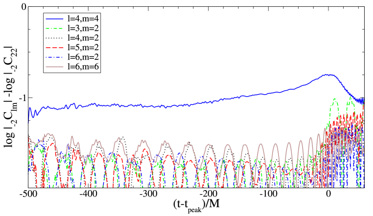
Figure 24: Magnitudes of several sub-dominate components of the $d=19$ waveform relative to the dominant $\ell=2,|m|=2$ component. Modes up to $\ell=6,|m|=6$ were extracted—those not present in the plot were several times (at least) smaller than any of the modes shown.

Appendix B Energy and Angular Momentum Flux

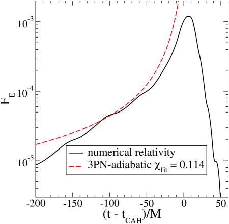
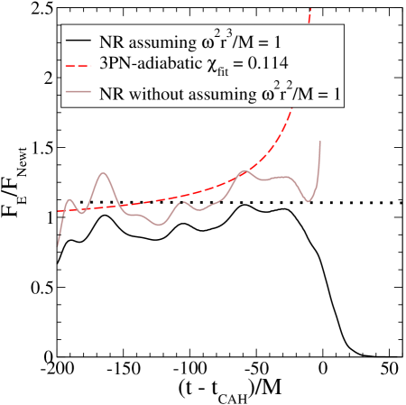
Figure 25: In the left plot we compare the GW energy fluxes of the numerical simulation and PN-adiabatic model when the best-fit for the orbital frequency is used (see Sec. IV.2). In the right plot, we show the same comparisons but we divide the fluxes by the Newtonian GW flux. For the numerical case we show the results assuming circular orbits, i.e., $F_{\rm Newt}=32/5\,\nu^{2}(M\omega)^{10/3}$ and not assuming circular orbits, i.e., $F_{\rm Newt}=32/5\,\nu^{2}(M\omega)^{6}\,(M/r)^{-4}$. The data refers to the $d=16$ run.

The GW energy flux emitted by a binary moving along an adiabatic sequence of circular orbits is currently known through 3.5PN order 35PNnospin for non-spinning BHs and through 2.5PN for spinning BHs 25PNspin . It reads

$$F_{\rm E} = {32\over 5}\nu^{2}(M\omega)^{10/3}\biggl{\{}1+\left(-\frac{1247}{336}-\frac{35}{12}\nu\right)(M\,\omega)^{2/3}+4\pi(M\,\omega)$$ (47)

$$+ \left(-\frac{44711}{9072}+\frac{9271}{504}\nu+\frac{65}{18}\nu^{2}\right)(M\,\omega)^{4/3}+\left(-\frac{8191}{672}-\frac{583}{24}\nu\right)\pi(M\,\omega)^{5/3}$$

$$+ \frac{(M\,\omega)}{G\,m^{2}}\left[-4S_{\ell}-\frac{5}{4}\frac{\delta M}{M}\Sigma_{\ell}\right]$$

$$+ \frac{(M\,\omega)^{5/3}}{G\,m^{2}}\left[\left(\frac{65}{14}+\frac{428}{63}\nu\right)S_{\ell}+\left(\frac{51}{16}-\frac{67}{28}\nu\right)\frac{\delta M}{M}\Sigma_{\ell}\right]$$

$$+ \left(\frac{6643739519}{69854400}+\frac{16}{3}\pi^{2}-\frac{1712}{105}C-\frac{856}{105}\ln(16~{}\!(M\,\omega))\right.$$

$$+ \left.\left[-\frac{134543}{7776}+\frac{41}{48}\pi^{2}\right]\nu-\frac{94403}{3024}\nu^{2}-\frac{775}{324}\nu^{3}\right)(M\,\omega)^{2}$$

$$+ \left(-\frac{16285}{504}+\frac{214745}{1728}\nu+\frac{193385}{3024}\nu^{2}\right)\pi(M\,\omega)^{7/3}\biggr{\}}\;.$$

The numerical energy flux is computed in terms of the mode amplitudes ${}_{-\!2}C_{\ell m}(t)$ as

$$\frac{dE}{dt}=\frac{1}{16\pi}\sum_{\ell m}{|D_{\ell m}(t)|^{2}},$$ (48)

where $D_{\ell m}(t)$ is a dimensionless first time integral of ${}_{-\!2}C_{\ell m}(t)$ defined by

$$D_{\ell m}(t)\equiv\frac{1}{M}\int_{0}^{t}{dt^{\prime}{}_{-\!2}C_{\ell m}(t^{\prime})}.$$ (49)

In the left panels of Figs. 25, 26, we compare the PN-adiabatic and numerical fluxes for the runs $d=16$ and $d=19$. We compute the PN-adiabatic flux from Eq. (47), using the best-fit $\omega$ derived in Sec. IV.2. To better pinpoint the differences, we show in the right panels of Figs. 25, 26, the GW energy fluxes normalized to the Newtonian GW flux, assuming the Keplerian relation $\omega^{2}r^{3}/M=1$ valid for circular orbits. In addition, we show a curve where the flux has been calculated without assuming the Keplerian relation. We notice that for the case $d=19$, except for the very first part of the evolution, the PN-adiabatic flux averages the numerical one until $\approx 30\mbox{--}50M$ before the CAH forms. For the case $d=16$, the PN-adiabatic flux computed from the best-fit PN-adiabatic $\omega$ always overestimates the numerical one.

Figures 25, 26 show that the frequency obtained by fitting the numerical frequency, as done in Sec. IV.2, not only provides a GW signal that matches the numerical one quite well, but also provides an energy flux that is consistent with the numerical energy flux. However, this study does not give hints on which analytical model and/or PN order best fits the numerical flux. We leave for future work a more detail study of the comparison between numerical and analytical energy and angular-momentum fluxes, which includes fully relaxing the assumption of circular orbits and comparisons with the Padé resummed fluxes.

In PN theory it is possible to show that the following relationship holds between the radiated angular momentum flux $dJ_{z}/dt$ and energy flux $dE/dt$ for circular orbits:

$$\frac{dE}{dt}=\omega\,\frac{dJ_{z}}{dt}\,.$$ (50)

The above equation is used in building the EOB equations of motion BD2 ; BCD . The numerical angular momentum flux is computed in terms of the mode amplitudes ${}_{-\!2}C_{\ell m}(t)$ as

$$\frac{dJ_{z}}{dt}=-\frac{M}{16\pi}\sum_{\ell m}{m\left({\rm Im}[D_{\ell m}(t)E^{*}_{\ell m}(t)]\right)},$$ (51)

where $E_{\ell m}(t)$ is a dimensionless second time integral of ${}_{-\!2}C_{\ell m}(t)$ defined by

$$E_{\ell m}(t)\equiv\frac{1}{M}\int_{0}^{t}{dtD_{\ell m}(t^{\prime})}.$$ (52)

In Figure 27 we plot these two quantities calculated from the angular momentum and energy fluxes of the numerical simulation, using the frequency $\omega_{D2}$ (23). The oscillations we see in the numerical $dJ_{z}/dt$ are, we believe, due in part to improper initial conditions in the double-time integral of $\Psi_{4}$ used to obtain $dJ_{z}/dt$ (we used initial conditions that are valid at $t=-\infty$); however, on average (50) appears to hold to a reasonable degree throughout the entire evolution.

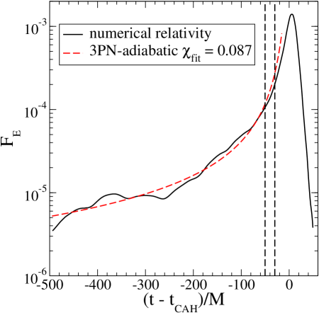
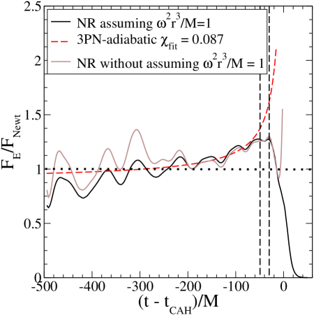
Figure 26: In the left plot we compare the GW energy fluxes of the numerical simulation and PN-adiabatic model when the best-fit for the orbital frequency is used (see Sec. IV.2). In the right plot, we show the same comparisons but we divide the fluxes by the Newtonian GW flux. For the numerical case we show the results assuming circular orbits, i.e., $F_{\rm Newt}=32/5\,\nu^{2}(M\omega)^{10/3}$ and not assuming circular orbits, i.e., $F_{\rm Newt}=32/5\,\nu^{2}(M\omega)^{6}\,(M/r)^{-4}$. The two vertical lines span the region in which a dynamical ISCO could exist. The data refers to the $d=19$ run.

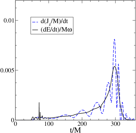
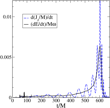
Figure 27: Comparison of $dJ_{z}/dt$ and $(dE/dt)/(M\omega)$ from numerical data for the $d=16$ and $d=19$ runs.

Appendix C Effect of extraction radius on measured waveform

There are many coordinate related issues in extracting GWs from the simulation, most of which have not been rigorously addressed for this set of runs. The issues can be summarized by the question how does the gauge used in the simulation affect the assumed relationship between $\Psi_{4}$ and the gravitational wave strain given in Eq. (14)?. Most certainly there are differences that decay by some power of $r$, as only in the limit as $r\rightarrow\infty$ is (14) strictly satisfied. To test whether such differences are present and estimate how significant they are, we can examine $rM\Psi_{4}(t,r,\theta,\phi)$, or equivalently ${}_{-2}C_{\ell m}(t,r)$ as defined in Eq. (17), as a function of extraction radius $r$. In the wave zone of a “good” coordinate system ${}_{-2}C_{\ell m}(t,r)={}_{-2}C_{\ell m}(t-r)$ for large $r$, and so by comparing the waveform at several extraction radii will give some hints as to the adequacy of the coordinates.

Figures 28–30 show two plots each of ${}_{-2}C_{2,2}(t,r)$ at four extraction radii, $r=12.5M,25M,37.5M$ and $50M$, for each of the three simulations (h/2 resolution). The plots on the left show the early part of the waveform, shifted by an appropriate amount in time assuming that the wave is propagating with unit velocity. As can be seen, going from an extraction radius of $37.5M$ to $50M$ the shifted waveforms all overlap quite closely, in consistency with wave-like propagation. However, these time-shifts do not give such a good match in the part of the waveform associated with the coalescence and ring-down of the binary. This is evident from the plots on the right, where now the time shift has been chosen to give the best possible phase overlap around peak amplitude. What these latter plots suggest is that the gauge changes by a small amount with time in the wave extraction regime of the simulation, and the amount of change is apparently correlated with the amplitude of the GWs being emitted.

These effects are summarized in Table 6, where we give the average coordinate propagation speeds between the different extraction radii during the inspiral and coalescence/merger portion of the signal. Another apparent gauge pathology seen in Figs. 28–30 is that near the peak amplitude the assumed $1/r$ decay in the wave amplitude [factored out in Eq. (17)] does not describe the situation as well as in the inspiral regime. This could happen (for example) if the coordinate sphere $r=r_{i}$ begins to deviate from a geometric sphere of radius $r_{i}$; such a change in gauge could also affect the coordinate velocity of the wave, and in fact the trend of decreasing amplitude with extraction radius is consistent with the decrease in wave speed (though cannot by itself account for all the change in velocity).

d=13	$v_{avg,inspiral}$	$v_{avg,peak}$
r=12.5M to 25M	—	0.84
r=25M to 37.5M	0.98	0.89
r=37.5M to 50M	0.98	0.93
d=16	$v_{avg,inspiral}$	$v_{avg,peak}$
r=12.5M to 25M	—	0.77
r=25M to 37.5M	0.99	0.85
r=37.5M to 50M	0.99	0.89
d=19	$v_{avg,inspiral}$	$v_{avg,peak}$
r=12.5M to 25M	—	0.71
r=25M to 37.5M	1.20	0.81
r=37.5M to 50M	1.00	0.86

Table 6: The average GW propagation speed between various extraction radii for the inspiral part of the wave and the coalescence/ring-down (“peak”) part—see Fig.’s 28 to 30

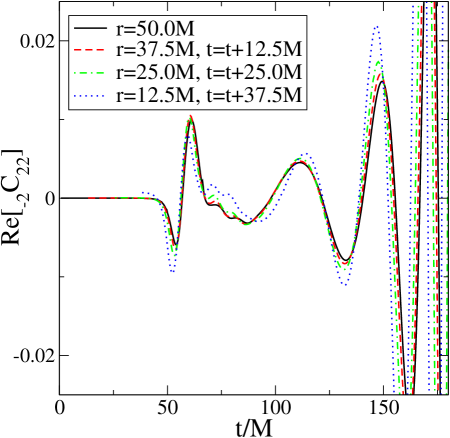
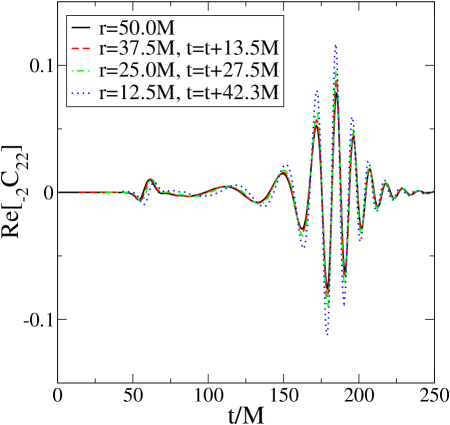
Figure 28: A component of the waveform of the d=13 (h/2) run measured at different extraction radii, and shifted in time to account for wave propagation speed. The figure to the left has time shifts assuming unit coordinate speed, which for large extraction radii seem to be a good assumption for the inspiral part of the wave though produce some mismatch around peak amplitude; the figure to the right depicts the time shift necessary to produce the best overlap about peak amplitude. See Fig’s 29 and 30 for similar plots for d=16 and d=19 respectively.

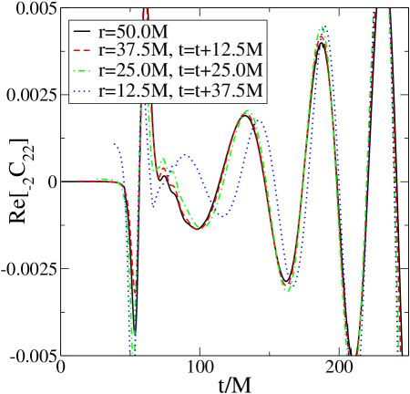
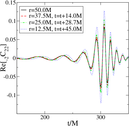
Figure 29: Time-shifted waveforms versus extraction radius for d=16 (see the caption describing the the corresponding $d=13$ plot in Fig.28)

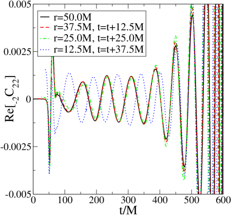
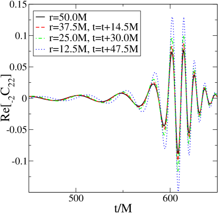
Figure 30: Time-shifted waveforms versus extraction radius for d=19 (see the caption describing the the corresponding $d=13$ plot in Fig.28)

Appendix D Tables

This appendix contains tables from the QNM ring-down analysis presented in Sec. V. Tables 7, 7 and 9 are fit parameters for the ${}_{-\!2}C_{22}$ component of the waveform from the $d=13,16$ and $19$ cases respectively; similarly Tables 10, 10 and 12 are fit parameters for the ${}_{-\!2}C_{32}$ component of the waveform for the same set of separations.

Table 7: Fit parameters for ${}_{-\!2}C_{22}$ for the $d=13$ case. $t_{r}/m$ denotes the time after the peak in $|{}_{-\!2}C_{22}|$ at which the fitting started.

	${\rm Re}[{}_{-\!2}C_{22}]$				${\rm Im}[{}_{-\!2}C_{22}]$
	$N=0$	$N=1$	$N=2$	$N=3$	$N=0$	$N=1$	$N=2$	$N=3$
$t_{r}/M$	20	8.5	-2.5	-6.5	17	4	-0.5	-9.5
$a/M_{f}$	0.725	0.723	0.737	0.736	0.725	0.735	0.733	0.748
$M_{f}/M$	0.943	0.939	0.950	0.949	0.943	0.948	0.945	0.959
${\cal C}_{2220}$	-0.143	-0.146	-0.140	-0.140	-0.145	-0.142	-0.144	-0.138
$\phi_{2220}$	1.65	1.60	1.60	1.58	1.66	1.59	1.57	1.58
${\cal C}_{2221}$	-	0.115	0.103	0.106	-	0.0985	0.120	0.0946
$\phi_{2221}$	-	1.25	0.975	0.959	-	1.07	0.979	0.946
${\cal C}_{2222}$	-	-	-0.0268	-0.0365	-	-	-0.0442	-0.0265
$\phi_{2222}$	-	-	0.580	0.501	-	-	0.688	0.445
${\cal C}_{2223}$	-	-	-	-0.00513	-	-	-	-0.00265
$\phi_{2223}$	-	-	-	3.14	-	-	-	3.04
$M\,\omega_{220}$	0.577	0.579	0.579	0.579	0.577	0.579	0.580	0.580
$M/\tau_{220}$	0.0845	0.0850	0.0834	0.0835	0.0847	0.0836	0.0841	0.0820
$M\,\omega_{221}$	-	0.567	0.568	0.568	-	0.569	0.569	0.569
$M/\tau_{221}$	-	0.257	0.252	0.252	-	0.253	0.254	0.248
$M\,\omega_{222}$	-	-	0.548	0.548	-	-	0.548	0.550
$M/\tau_{222}$	-	-	0.425	0.423	-	-	0.428	0.417
$M\,\omega_{223}$	-	-	-	0.520	-	-	-	0.522
$M/\tau_{223}$	-	-	-	0.602	-	-	-	0.591

Table 8: Fit parameters for ${}_{-\!2}C_{22}$ for the $d=16$ case. $t_{r}/m$ denotes the time after the peak in $|{}_{-\!2}C_{22}|$ at which the fitting started.

	${\rm Re}[{}_{-\!2}C_{22}]$				${\rm Im}[{}_{-\!2}C_{22}]$
	$N=0$	$N=1$	$N=2$	$N=3$	$N=0$	$N=1$	$N=2$	$N=3$
$t_{r}/M$	20.5	8.5	2.5	-2.5	19	10	0	-4
$a/M_{f}$	0.729	0.726	0.730	0.731	0.728	0.722	0.736	0.739
$M_{f}/M$	0.947	0.942	0.944	0.945	0.947	0.939	0.949	0.951
${\cal C}_{2220}$	-0.151	-0.155	-0.153	-0.153	-0.152	-0.158	-0.152	-0.150
$\phi_{2220}$	1.70	1.66	1.63	1.62	1.71	1.67	1.63	1.62
${\cal C}_{2221}$	-	0.146	0.164	0.169	-	0.151	0.147	0.153
$\phi_{2221}$	-	1.13	0.922	0.894	-	1.26	0.920	0.811
${\cal C}_{2222}$	-	-	-0.0971	-0.126	-	-	-0.0666	-0.0959
$\phi_{2222}$	-	-	0.636	0.548	-	-	0.559	0.278
${\cal C}_{2223}$	-	-	-	0.0444	-	-	-	0.0263
$\phi_{2223}$	-	-	-	0.325	-	-	-	-0.133
$M\,\omega_{220}$	0.577	0.578	0.579	0.579	0.577	0.578	0.579	0.580
$M/\tau_{220}$	0.0840	0.0846	0.0842	0.0842	0.0841	0.0851	0.0836	0.0833
$M\,\omega_{221}$	-	0.567	0.568	0.568	-	0.566	0.568	0.569
$M/\tau_{221}$	-	0.256	0.254	0.254	-	0.257	0.252	0.251
$M\,\omega_{222}$	-	-	0.547	0.547	-	-	0.548	0.549
$M/\tau_{222}$	-	-	0.429	0.429	-	-	0.426	0.424
$M\,\omega_{223}$	-	-	-	0.518	-	-	-	0.520
$M/\tau_{223}$	-	-	-	0.607	-	-	-	0.600

Table 9: Fit parameters for ${}_{-\!2}C_{22}$ for the $d=19$ case. $t_{r}/M$ denotes the time after the peak in $|{}_{-\!2}C_{22}|$ at which the fitting started.

	${\rm Re}[{}_{-\!2}C_{22}]$				${\rm Im}[{}_{-\!2}C_{22}]$
	$N=0$	$N=1$	$N=2$	$N=3$	$N=0$	$N=1$	$N=2$	$N=3$
$t_{r}/M$	21.5	7.5	1	-4	20.5	7	-1.5	-5.5
$a/M_{f}$	0.707	0.709	0.712	0.712	0.705	0.705	0.721	0.723
$M_{f}/M$	0.948	0.947	0.948	0.947	0.946	0.943	0.955	0.955
${\cal C}_{2220}$	0.170	0.172	0.171	0.171	0.173	0.176	0.168	0.168
$\phi_{2220}$	2.46	2.41	2.39	2.39	2.47	2.40	2.39	2.37
${\cal C}_{2221}$	-	-0.158	-0.179	-0.183	-	-0.177	-0.160	-0.167
$\phi_{2221}$	-	1.97	1.81	1.80	-	1.97	1.79	1.71
${\cal C}_{2222}$	-	-	0.0859	0.107	-	-	0.0590	0.0824
$\phi_{2222}$	-	-	157	1.50	-	-	1.47	1.26
${\cal C}_{2223}$	-	-	-	-0.0273	-	-	-	-0.0160
$\phi_{2223}$	-	-	-	1.22	-	-	-	0.815
$M\,\omega_{220}$	0.566	0.567	0.568	0.568	0.565	0.567	0.568	0.569
$M/\tau_{220}$	0.0850	0.0850	0.0848	0.0848	0.0852	0.0855	0.0837	0.0836
$M\,\omega_{221}$	-	0.555	0.556	0.556	-	0.555	0.557	0.557
$M/\tau_{221}$	-	0.257	0.256	0.256	-	0.258	0.253	0.253
$M\,\omega_{222}$	-	-	0.534	0.534	-	-	0.535	0.536
$M/\tau_{222}$	-	-	0.432	0.432	-	-	0.427	0.426
$M\,\omega_{223}$	-	-	-	0.505	-	-	-	0.507
$M/\tau_{223}$	-	-	-	0.613	-	-	-	0.603

Table 10: Fit parameters for ${}_{-\!2}C_{32}$ for the $d=13$ case. $t_{r}/M$ denotes the time after the peak in $|{}_{-\!2}C_{22}|$ at which the fitting started.

	${\rm Re}[{}_{-\!2}C_{32}]$			${\rm Im}[{}_{-\!2}C_{32}]$
	$N=0$	$N=1$	$N=2$	$N=0$	$N=1$	$N=2$
$t_{r}/M$	16	-0.5	-4.5	14.5	-2	10
$a/M_{f}$	0.731	0.753	0.721	0.704	0.738	0.710
$M_{f}/M$	0.947	0.955	0.921	0.931	0.953	0.925
${\cal C}_{3220}$	-0.00753	-0.00730	-0.00868	-0.00755	-0.00721	-0.00804
$\phi_{3220}$	1.53	1.33	1.16	0.915	0.816	0.720
${\cal C}_{3320}$	0.00599	0.00563	0.00628	0.00844	0.00734	0.00811
$\phi_{3320}$	2.77	2.61	2.14	2.86	2.89	2.61
${\cal C}_{3221}$	-	0.00822	0.0272	-	0.00787	0.0142
$\phi_{3221}$	-	0.749	1.17	-	0.720	0.872
${\cal C}_{3321}$	-	-0.00592	-0.0188	-	-0.007528	-0.0121
$\phi_{3321}$	-	1.56	0.298	-	2.16	1.48
${\cal C}_{3222}$	-	-	-0.0153	-	-	-0.00235
$\phi_{3222}$	-	-	2.46	-	-	1.98
${\cal C}_{3322}$	-	-	-0.0127	-	-	-0.00201
$\phi_{3322}$	-	-	1.71	-	-	3.10
$M\,\omega_{220}$	0.578	0.585	0.589	0.574	0.578	0.580
$M/\tau_{220}$	0.0840	0.0821	0.0868	0.0866	0.0831	0.0869
$M\,\omega_{320}$	0.817	0.820	0.836	0.819	0.815	0.827
$M/\tau_{320}$	0.0874	0.0855	0.0904	0.0902	0.0865	0.0905
$M\,\omega_{221}$	-	0.575	0.577	-	0.567	0.568
$M/\tau_{221}$	-	0.248	0.262	-	0.251	0.263
$M\,\omega_{321}$	-	0.813	0.828	-	0.807	0.818
$M/\tau_{321}$	-	0.258	0.273	-	0.261	0.273
$M\,\omega_{222}$	-	-	0.555	-	-	0.546
$M/\tau_{222}$	-	-	0.443	-	-	0.443
$M\,\omega_{322}$	-	-	0.812	-	-	0.802
$M/\tau_{322}$	-	-	0.462	-	-	0.462

Table 11: Fit parameters for ${}_{-\!2}C_{32}$ for the $d=16$ case. $t_{r}/m$ denotes the time after the peak in $|{}_{-\!2}C_{22}|$ at which the fitting started.

	${\rm Re}[{}_{-\!2}C_{32}]$			${\rm Im}[{}_{-\!2}C_{32}]$
	$N=0$	$N=1$	$N=2$	$N=0$	$N=1$	$N=2$
$t_{r}/M$	15.5	3.5	-5	14.5	0.5	-5
$a/M_{f}$	0.740	0.718	0.722	0.731	0.7.22	0.729
$M_{f}/M$	0.952	0.936	0.922	0.944	0.928	0.918
${\cal C}_{3220}$	-0.00903	-0.00990	-0.107	-0.00846	-0.00932	-0.0101
$\phi_{3220}$	1.57	1.61	1.25	1.32	1.05	0.828
${\cal C}_{3320}$	0.00835	0.00919	0.00907	0.00981	0.0102	0.00988
$\phi_{3320}$	2.88	2.75	2.28	2.88	2.49	2.20
${\cal C}_{3221}$	-	0.00999	0.0350	-	0.0216	0.0413
$\phi_{3221}$	-	1.91	1.37	-	0.911	0.918
${\cal C}_{3321}$	-	-0.0189	-0.0265	-	-0.0192	-0.0273
$\phi_{3321}$	-	2.14	0.649	-	1.34	0.404
${\cal C}_{3222}$	-	-	-0.0179	-	-	-0.017
$\phi_{3222}$	-	-	2.67	-	-	2.10
${\cal C}_{3322}$	-	-	-0.0149	-	-	-0.0137
$\phi_{3322}$	-	-	2.08	-	-	1.79
$M\,\omega_{220}$	0.579	0.578	0.589	0.580	0.588	0.595
$M/\tau_{220}$	0.0831	0.0856	0.0867	0.0842	0.0859	0.0867
$M\,\omega_{320}$	0.817	0.821	0.835	0.820	0.833	0.841
$M/\tau_{320}$	0.0865	0.0891	0.0903	0.0877	0.0895	0.0903
$M\,\omega_{221}$	-	0.566	0.577	-	0.576	0.583
$M/\tau_{221}$	-	0.259	0.262	-	0.260	0.262
$M\,\omega_{321}$	-	0.813	0.827	-	0.824	0.833
$M/\tau_{321}$	-	0.269	0.273	-	0.270	0.273
$M\,\omega_{222}$	-	-	0.555	-	-	0.561
$M/\tau_{222}$	-	-	0.442	-	-	0.442
$M\,\omega_{322}$	-	-	0.811	-	-	0.817
$M/\tau_{322}$	-	-	0.461	-	-	0.461

Table 12: Fit parameters for ${}_{-\!2}C_{32}$ for the $d=19$ case. $t_{r}/M$ denotes the time after the peak in $|{}_{-\!2}C_{22}|$ at which the fitting started.

	${\rm Re}[{}_{-\!2}C_{32}]$			${\rm Im}[{}_{-\!2}C_{32}]$
	$N=0$	$N=1$	$N=2$	$N=0$	$N=1$	$N=2$
$t_{r}/M$	13.5	0	-5	12.5	-0.5	-6
$a/M_{f}$	0.729	0.723	0.706	0.730	0.713	0.704
$M_{f}/M$	0.964	0.956	0.937	0.961	0.944	0.930
${\cal C}_{3220}$	0.00931	0.00978	0.0107	0.00742	0.00823	0.00896
$\phi_{3220}$	2.40	2.34	2.23	2.10	2.02	1.91
${\cal C}_{3320}$	0.00704	0.00729	0.00782	0.00830	0.00880	0.00907
$\phi_{3320}$	0.471	0.326	0.493	0.431	0.218	-0.0134
${\cal C}_{3221}$	-	-0.00974	-0.0210	-	-0.0148	-0.0259
$\phi_{3221}$	-	2.05	2.23	-	1.69	1.91
${\cal C}_{3321}$	-	0.00961	0.0187	-	0.0137	0.0225
$\phi_{3321}$	-	2.58	1.77	-	2.26	1.59
${\cal C}_{3222}$	-	-	-0.00750	-	-	-0.0853
$\phi_{3222}$	-	-	0.442	-	-	0.0885
${\cal C}_{3322}$	-	-	-0.00795	-	-	-0.00882
$\phi_{3322}$	-	-	0.291	-	-	0.0739
$M\,\omega_{220}$	0.566	0.568	0.571	0.569	0.571	0.574
$M/\tau_{220}$	0.0826	0.0835	0.0860	0.0828	0.0850	0.0866
$M\,\omega_{320}$	0.802	0.805	0.815	0.805	0.812	0.819
$M/\tau_{320}$	0.0860	0.0870	0.0896	0.0862	0.0886	0.0902
$M\,\omega_{221}$	-	0.557	0.559	-	0.559	0.562
$M/\tau_{221}$	-	0.252	0.260	-	0.227	0.262
$M\,\omega_{321}$	-	0.797	0.806	-	0.804	0.811
$M/\tau_{321}$	-	0.263	0.271	-	0.268	0.273
$M\,\omega_{222}$	-	-	0.537	-	-	0.539
$M/\tau_{222}$	-	-	0.439	-	-	0.442
$M\,\omega_{322}$	-	-	0.790	-	-	0.794
$M/\tau_{322}$	-	-	0.458	-	-	0.461

Appendix E Results for $d=13$

This appendix contains some figures showing results from the $d=13$ run that were excluded from the main text for brevity. Figure 31 shows orbital angular frequencies extracted using several methods (Sec. IV.1), and a comparison of the numerical and NQC inspiral waveforms (Sec. IV.1), Fig. 32 shows a comparison of frequencies and waveform components between NR and various analytical counterparts (Sec. IV.2), Fig. 33 shows results from QNM extraction (Sec. V), and Fig. 34 plots the dominant frequencies during the ring-down phase (Sec. V) and identifies features of the merger (Sec. VI).

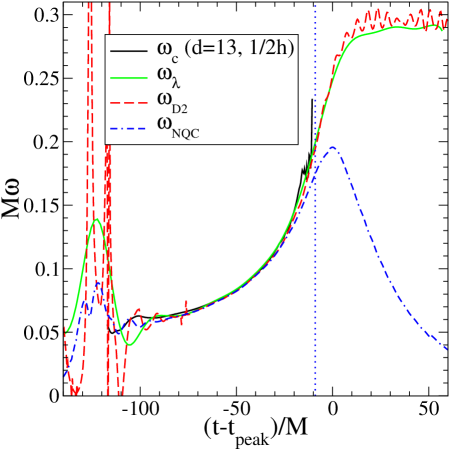
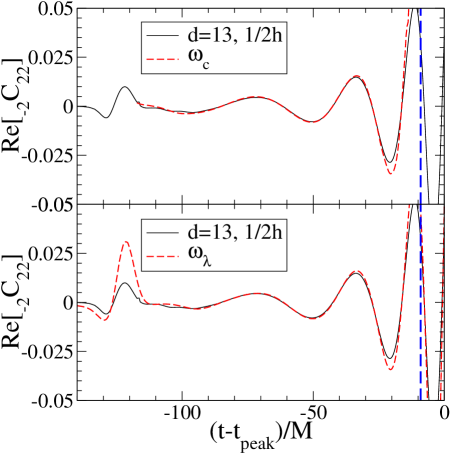
Figure 31: (left panel) Orbital angular frequencies for the $d=13$ case. See Fig. 7 for a full description. (right panel) Comparison of numerical and NQC inspiral waveforms for the $d=13$. See Fig. 8 for a full description.

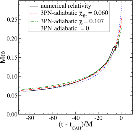
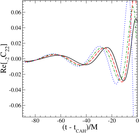
Figure 32: (left panel) Comparison of the NR and three analytical orbital frequencies— see Fig. 10 for a full description. (right panel) Comparison of the NR and analytical ${\rm Re}[{}_{-\!2}C_{22}]$—see Fig. 11 for a full description.

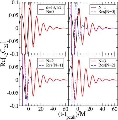
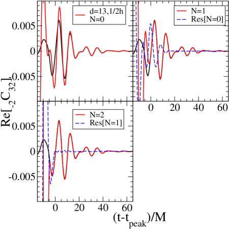
Figure 33: The left panel shows a comparison of numerical and QNM ${}_{-\!2}C_{22}$ ring-down waveforms for $d=13$—see Fig. 15 for a full description. The right panel shows a comparison of numerical and QNM ${}_{-\!2}C_{32}$ ring-down waveforms for $d=13$—see Fig. 16 for a full description.

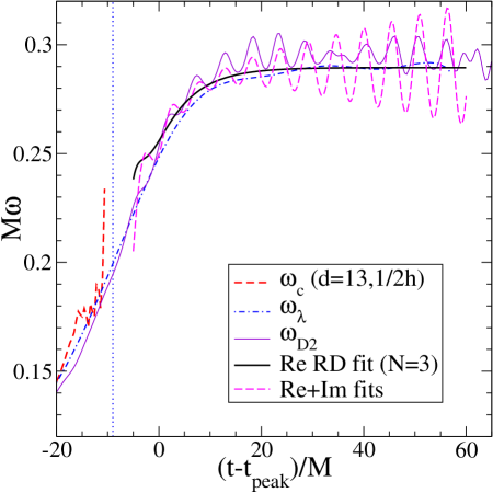
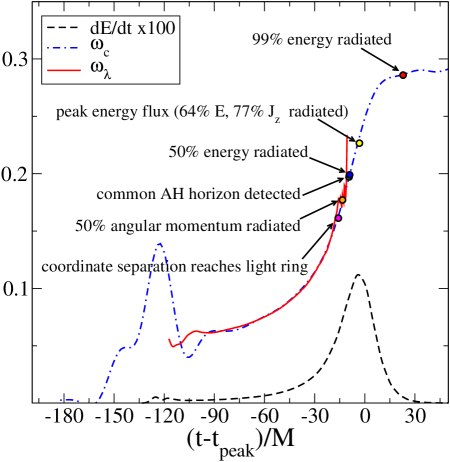
Figure 34: (left panel) Dominant frequencies during the ring down for the $d=13$ case evaluated using several methods. See Fig. 17 for a full description. (right panel) Features of the $d=13$ merger phase. See Fig. 18 for a full description.

References

- (1) A. Abramovici et al., Science 256, 325 (1992); http://www.ligo.caltech.edu.
- (2) H. Lück et al., Class. Quant. Grav. 14, 1471 (1997); http://www.geo600.uni-hannover.de.
- (3) M. Ando et al., Phys. Rev. Lett. 86, 3950 (2001); http://tamago.mtk.nao.ac.jp.
- (4) B. Caron et al., Class. Quant. Grav. 14, 1461 (1997); http://www.virgo.infn.it.
- (5) F. Pretorius, Phys. Rev. Lett. 95, 121101 (2005).
- (6) J. Baker, J. Centrella, D. Choi, M. Koppitz, J. van Meter, Phys. Rev. Lett. 96, 111102 (2006).
- (7) M. Campanelli, C.O. Lousto, P.Marronetti, and Y. Zlochower, Phys. Lett. 96, 111101 (2006);
- (8) F. Herrmann, D. Shoemaker and P. Laguna, submitted to Phys. Rev. Lett., gr-qc/0601026.
- (9) U. Sperhake, submitted to Phys. Rev. D., gr-qc/0606079.
- (10) H. Friedrich, Commun. Math. Phys 100, 525 (1985)
- (11) D. Garfinkle, Phys.Rev. D 65, 044029 (2002)
- (12) B. Szilagyi, B. G. Schmidt and J. Winicour, Phys. Rev. D 65, 064015 (2002)
- (13) C. Gundlach, J. M. Martin-Garcia, G. Calabrese and I. Hinder, Class. Quant. Grav. 22, 3767 (2005).
- (14) O. Brodbeck, S. Frittelli, P. Hubner and O. A. Reula, J. Math. Phys. 40, 909 (1999)
- (15) L. Lindblom, M. A. Scheel, L. E. Kidder,R. Owen and O. Rinne, Class. Quant. Grav. 23, S447(2006).
- (16) M. A. Scheel, H .P. Pfeiffer, L. Lindblom, L. E. Kidder, O. Rinne and S. A. Teukolsky, gr-qc/0607056 (2006)
- (17) B. Szilagyi as presented at the New Frontiers in Numerical Relativity workshop, Golm (2006).
- (18) T. Nakamura, K. Oohara and Y. Kojima, Prog. Theor. Phys. Suppl. 90, 1 (1987)
- (19) M. Shibata and T. Nakamura, Phys. Rev. D 52, 5428 (1995)
- (20) T. W. Baumgarte and S.L. Shapiro, Phys. Rev. D 59, 024007 (1999)
- (21) B. Brügmann, Int. J. Mod. Phys. D 8, 85 (1999)
- (22) B. Brügmann, as presented at the New Frontiers in Numerical Relativity workshop, Golm (2006).
- (23) P.Marronetti, as presented at the New Frontiers in Numerical Relativity workshop, Golm (2006).
- (24) D. Pollney, as presented at the New Frontiers in Numerical Relativity workshop, Golm (2006).
- (25) L. Blanchet, T. Damour, G. Esposito-Farese and B.R. Iyer, Phys. Rev. Lett. 93, 091101 (2004).
- (26) See, e.g., L. Blanchet, Living Rev. Rel. 5, 3 (2002).
- (27) A. Buonanno and T. Damour, Phys. Rev. D 59, 084006 (1999).
- (28) A. Buonanno and T. Damour, Phys. Rev. D 62, 064015 (2000).
- (29) A. Buonanno and T. Damour, Proceedings of IXth Marcel Grossmann Meeting (Rome, July 2000), gr-qc/0011052.
- (30) T. Damour, P. Jaranowski and G. Schäfer, Phys. Rev. D 62, 084011 (2000).
- (31) T. Damour, Phys. Rev. D 64, 124013 (2001).
- (32) A. Buonanno, Y. Chen and T. Damour, Phys. Rev. D 74, 104005 (2006).
- (33) T. Damour, B.R. Iyer and B.S. Sathyaprakash, Phys. Rev. D 57, 885 (1998).
- (34) J. Baker, J. Centrella, D. Choi, M. Koppitz, J. van Meter, Phys. Rev. D 73, 104002 (2006).
- (35) C.V. Vishveshwara, Nature 227, 936 (1970).
- (36) M. Davis, R. Ruffini, W.H. Press and R.H. Price, Phys. Rev. Lett. 27, 1466 (1971); M. Davis, R. Ruffini and J. Tiomno, Phys. Rev. D 5, 2932 (1972).
- (37) W. Press, Astrophys J. Letters 170, L105 (1971).
- (38) S. Chandrasekhar and S. Detweiler, Proc. R. Soc. Lond. A 344, (1975) 441.
- (39) B. Mashhoon, Phys. Rev. D 31, 290 (2005).
- (40) G. B. Cook and H. P. Pfeiffer, Phys. Rev. D 70, 104016 (2004).
- (41) M. Caudill, G. B. Cook, J. D. Grigsby, and H. P. Pfeiffer, Phys. Rev. D 74, 064011 (2006).
- (42) H. P. Pfeiffer L. E. Kidder, M. S. Scheel, and S. A. Teukolsky, Comp. Phys. Comm. 152, 253 (2003).
- (43) http://www.tapir.caltech.edu/~harald/PublicID/
- (44) H. P. Pfeiffer and J. W. York, Jr., Phys. Rev. D 67, 044022 (2003).
- (45) J. W. York, Jr., Phys. Rev. Lett. 82, 1350 (1999).
- (46) E. Gourgoulhon, P. Grandclément, and S. Bonazzola, Phys. Rev. D 65, 044020 (2002).
- (47) P. Grandclément, E. Gourgoulhon and S. Bonazzola, Phys. Rev. D 65, 044021 (2002).
- (48) G. B. Cook, Phys. Rev. D 50, 5025 (1994).
- (49) G. B. Cook, Phys. Rev. D 65, 084003 (2002).
- (50) T. Damour, E. Gourgoulhon and P. Grandclément, Phys. Rev. D 66, 024007 (2002).
- (51) L. Blanchet, Phys. Rev. D 65, 124009 (2002).
- (52) E. Berti, S. Iyer, and C. Will, Phys. Rev. D 74, 061503(R) (2006).
- (53) M. Miller, Phys. Rev. D 69, 124013 (2004).
- (54) F. Pretorius, Class. Quant. Grav. 22 425, (2005)
- (55) F. Pretorius, Class. Quant. Grav. 23, S529 (2006).
- (56) A. Lichnerowicz, J. Math. Pures Appl. 23, 37 (1944)
- (57) R. Arnowitt, S. Deser and C.W. Misner, in Gravitation: An Introduction to Current Research, ed. L. Witten, New York, Wiley (1962)
- (58) Y. Choquet-Bruhat, in Gravitation: An Introduction to Current Research, ed. L. Witten, New York, Wiley (1962)
- (59) J. W. York, in Sources of Gravitational Radiation, ed. L. Smarr, Seattle, Cambridge University Press (1978)
- (60) D. Christodoulou, Phys. Rev. Lett. 25, 1596 (1970); D. Christodoulou and R. Ruffini, Phys. Rev. D 4, 3552 (1971).
- (61) A. Nerozzi, M. Bruni, V Re and L. M. Burko, Phys. Rev. D 73, 044020 (2006)
- (62) A. Nerozzi, C. Beetle, M. Bruni, L. M. Burko and D. Pollney, Phys. Rev. D 72, 024014 (2005)
- (63) T. Baumgarte, P. R. Brady, L. Lehner and F. Pretorius, in preparation
- (64) M. Campanelli, C.O. Lousto and Y. Zlochower, Phys. Rev. D 73, 061501 (2006);
- (65) M. Campanelli, C.O. Lousto and Y. Zlochower, Phys. Rev. D 74, 041501 (2006)
- (66) L. E. Kidder, L. Lindblom, H. P. Pfeiffer and M. Scheel as presented at the New Frontiers in Numerical Relativity workshop, Golm (2006).
- (67) S.R. Brandt and E. Seidel, Phys.Rev.D 52, 870 (1995)
- (68) A. Ashtekar and B. Krishnan Living Rev.Rel. 7, 10 (2004)
- (69) T. Mora and C. Will, Phys. Rev. D 66, 101501 (2002); 69, 104021 (2004).
- (70) G. Faye, L. Blanchet, A. Buonanno, in press on Phys. Rev. D, gr-qc/0606139; L. Blanchet, A. Buonanno and G. Faye, in press on Phys. Rev. D, gr-qc/0606140.
- (71) L. Blanchet, G. Faye, B.R. Iyer and B. Joguet, Phys. Rev. D 65, 061501(R) (2002); Erratum Phys. Rev. D 71, 129902 (2005).
- (72) L. Blanchet, B.R. Iyer, C.M. Will and A. G. Wiseman, Class. Quant. Grav. 13, 575 (1996).
- (73) K.G. Arun, L. Blanchet, B.R. Iyer and M.S.S. Qusailah, Class. Quant. Grav. 21, 3771 (2004).
- (74) E. W. Leaver, Proc. R. Soc. Lond. A 402, (1985) 285.
- (75) F. Echeverria, Phys. Rev. D 40, 3194 (1997).
- (76) E. Berti, V. Cardoso and C. Will, Phys. Rev. D 73, 064030 (2006).
- (77) E. N. Dorband, E. Berti, P. Diener, E. Schnetter, and M. Tiglio, gr-qc/0608091 (2006).
- (78) W. H. Press and S. A. Teukolsky, Ap. J. 185, 649 (1973).
- (79) R.H. Price and J. Pullin, Phys. Rev. Lett. 72, 3297 (1994).
- (80) A. M. Abraham and G.B. Cook, Phys. Rev. D 50, R2364 (1994).
- (81) R.J. Gleiser, C.O. Nicasio, R. Price and J. Pullin, Class. Quant. Grav. 13, L117 (1996); Phys. Rev. Lett. 77, 4483 (1996).
- (82) J. Pullin, The close limit of colliding black holes: an update, Talk given at the Yukawa International Symposium at Kyoto, Japan, 1999 gr-qc/9909021 and references therein.
- (83) P. Anninos, D. Hobill, E. Seidel, L. Smarr and W.M. Suen, Phys. Rev. Lett. 71, 2851 (1993).
- (84) Z. Andrade and R. H. Price, Phys.Rev.D 56, 6336 (1997).
- (85) T. Damour, A. Nagar and A. Tartaglia, (in preparation).
- (86) J. Baker et al., (personal communication).
- (87) E. Berti, A. Buonanno, and C. Will, Phys. Rev. D 71, 084025 (2005).
- (88) A. Buonanno, Y. Chen and M. Vallisneri, Phys. Rev. D 67, 024016 (2002); Erratum Phys. Rev. D 74, 029903 (2006).
- (89) A. Buonanno, Y. Chen and M. Vallisneri, Phys. Rev. D 67, 104025 (2002); Erratum Phys. Rev. D 74, 029904 (2006).
- (90) T. Damour, P. Jaranowski and G. Schäfer, Phys. Lett. B 513, 147 (2001).
- (91) P. Jaranowski and G. Schäfer, Phys. Rev. D 57, 7274 (1998); 63 029902(E) (2001).
- (92) J. Baker, B. Brügmann, M. Campanelli, C.O. Lousto and R. Takahashi, Phys. Rev. Lett. 87, 121103 (2001).
- (93) E.E. Flanagan and S.A. Hughes, Phys. Rev. D 57, 4535 (1998).