Isolated, slowly evolving, and dynamical trapping horizons:
geometry and mechanics from surface deformations

Abstract

We study the geometry and dynamics of both isolated and dynamical trapping horizons by considering the allowed variations of their foliating two-surfaces. This provides a common framework that may be used to consider both their possible evolutions and their deformations as well as derive the well-known flux laws. Using this framework, we unify much of what is already known about these objects as well as derive some new results. In particular we characterize and study the “almost-isolated” trapping horizons known as slowly evolving horizons. It is for these horizons that a dynamical first law holds and this is analogous and closely related to the Hawking-Hartle formula for event horizons.

I Introduction

Fundamentally, there are two ways to characterize a black hole. The first focuses on causal structure and says that a point in an asymptotically flat spacetime is inside a black hole if no signal from that point can reach future null infinity (see, for example, hawkellis ). The boundary of the black hole region is the event horizon. This is an intuitive definition but at the same time is teleological and so highly non-local — one must trace all causal curves from a point before deciding whether or not it lies inside a black hole. By this definition neither large spacetime curvatures nor singularities are necessary for black hole existence.

In contrast, the second characterization is quasilocal and geometric, saying that a point in spacetime is inside a black hole if it lies on a trapped surface. Such surfaces, from which both future directed null expansions are everywhere negative, are indicative of large spacetime curvature and so this definition directly makes the association between strong gravitational fields and black holes. It is also directly connected to spacetime singularities as the existence of a trapped surface is sufficient to imply the existence of a spacetime singularity penrose .

Traditionally, the second viewpoint inspired the definition of an apparent horizon. Given a Cauchy surface, the trapped region is defined as the (closure of the) union of all the trapped surfaces contained in that slice of spacetime. The apparent horizon is then the (two-dimensional) boundary of the trapped region hawkellis . Correspondingly, if a region of spacetime is foliated by Cauchy surfaces, then one can locate the apparent horizon on each slice and so define a time-evolved (three-dimensional) version of the apparent horizon. Often this is also referred to as the apparent horizon.

For any given foliation of a spacetime, most trapped surfaces will not lie in the specified slices. Thus the time-evolved apparent horizon is defined by only a subset of the total number of trapped surfaces and so is certainly slicing dependent and contained in the “total” trapped region. The time-evolved apparent horizons defined by various foliations will typically intersect each other multiple times and also will usually have fully trapped surfaces lying partially outside of them (see for example waldiyer ; eardley ; BadApVar for discussions on these points).

By definition, an apparent horizon is a boundary between regions containing trapped and untrapped surfaces. As such, it is no surprise that it is marginally outer trapped — that is the expansion, $\theta_{(\ell)}$, of its outward null normal, $\ell$, vanishes hawkellis . Now, while it is certainly not true that all such surfaces will be apparent horizons, in practical terms it is clearly easier to find the marginally outer trapped surfaces (MOTS) and then identify apparent horizon candidates, rather than try to proceed by first identifying all trapped surfaces. This is the approach taken in numerical relativity (see for example thomas ) and in fact in that field “apparent horizon” is usually understood to mean the outermost MOTS.

Other properties can also be expected from an apparent horizon. First if there are fully trapped surfaces “just inside” the apparent horizon, then there should exist arbitrarily small inward deformations generated by some spacelike vector field $X^{a}$ under which the outward expansion becomes negative, i.e. $\delta_{X}\theta_{(\ell)}<0$. Furthermore, by continuity with the fully trapped surfaces, the expansion $\theta_{(n)}$ of the inward-pointing null normal $n$ should be negative on the apparent horizon. Over a decade ago, Hayward formalized this intuition in his definition of trapping horizons hayward . Here, we will be mainly interested in future outer trapping horizons (FOTHs) which are three-surfaces that may be foliated by two-surfaces with $\theta_{(\ell)}=0$, $\theta_{(n)}<0$ and $\delta_{n}\theta_{(\ell)}<0$. Although these will include most time-evolved apparent horizons, the focus has now shifted to the three-dimensional horizon surface itself. There is no reference to a foliation of the full spacetime.

Marginally trapped surfaces are practical as they may be (relatively) easily identified in simulations as well as studied with standard geometric tools. However, they are also philosophically appealing as, in contrast to event horizons, their evolution is causal. As such, this idea of studying the “boundary” of a trapped region without first finding a corresponding bulk has become increasingly popular in the last few years. Apart from the further studies of trapping horizons haywardPert ; haywardFlux there are closely related programmes such as isolated horizons which identify and study equilibrium states isoPRL ; LewIso ; isoMech ; isoGeom ; BadIsoNum , dynamical horizons which correspond to non-trivially evolving horizons ak ; theBeast ; gregabhay ; mttpaper ; ams ; GourgFlux ; Gourgoulhon:2006uc ; KrishNum ; bart ; matt ; MK , and slowly evolving horizons which are “almost isolated” trapping horizons prl ; billsPaper . For reviews of the field see, for example akRev ; GourgRev ; meRev .

Trapping and dynamical horizons each come equipped with a preferred foliation into two-surfaces. It is this foliation which is used to define the null normals and hence the expansions. In this paper we will focus on variations of these two-surfaces as a route to a better understanding of the existence, evolutions and deformations of the full three-dimensional horizons. Given a vector field $X=A\ell-Bn$ (where $A$ and $B$ are functions) normal to a horizon cross-section, the corresponding variations are generated by $\delta_{X}$. Particularly important is the variation $\delta_{X}\theta_{(\ell)}$ which turns out to be a second-order elliptic operator in $B$ that is defined by the intrinsic and extrinsic geometry of the two-surface along with components of the Einstein tensor. The techniques used are similar to those described in ams ; Andersson:2005me , however the emphasis is somewhat different. In those papers, the focus was on two-dimensional MOTS in a three-dimensional slice of space-time, whereas we consider general deformations of the two-surface in the full four-dimensional spacetime.

Solutions of $\delta_{X}\theta_{(\ell)}=0$ generate both the evolution and the possible deformations of FOTHs. A judicious application of a maximum principle to the resulting elliptic partial differential equation is a key to both deriving new results about these horizons and also unifying much of the existing knowledge under a common formalism. Among other results, this technique will be used to show that any foliation of an isolated FOTH may be freely deformed (a well-known result) while the foliation of dynamical FOTH is rigid (a related version of this was first shown in gregabhay ). Conversely we will see that an isolated FOTH is rigid against normal deformations (it may only be deformed into itself) while this is definitely not true for a dynamical FOTH. However, the allowed deformations in the dynamical case are strongly restricted by rules that are consistent with, although slightly different from, those seen in gregabhay .

Results from black hole physics also follow from the deformation equations. Apart from the second law of horizon dynamics hayward ; ak ; ams and angular momentum flux laws by ; ak ; GourgFlux we will examine slowly evolving horizons in some detail prl ; billsPaper . In particular we will explain how a horizon may be invariantly characterized as “almost” isolated. From this definition we will examine the circumstances under which a FOTH has a well-defined and slowly varying surface gravity and derive the first law for slowly evolving horizons. The related flux laws for event and dynamical horizons also follow from the variation equations.

The plan of the paper is as follows. We begin, in Section II, by considering the geometry of general spacelike two-surfaces embedded in four-dimensional spacetimes and study how that geometry changes if the surfaces are deformed . From there we specialize to two-surfaces that satisfy $\theta_{(\ell)}=0$, $\theta_{(n)}<0$, and $\delta_{n}\theta_{(\ell)}<0$ and study the properties of deformations that preserve those conditions. This is done in Section III. Next, in Section IV, we apply these results to gain a better understanding of isolated, dynamical, and future outer trapping horizons. With this general understanding in hand we turn to a more specialized study of slowly evolving horizons in Section V. Finally we compare the flux laws for slowly evolving horizons to the corresponding ones for dynamical and event horizons in Section VI. Numerous technical results are found in Appendices A–C.

II Two-surfaces and their deformations

To begin, we review the differential geometry of two-surfaces embedded in four-dimensional spacetimes. Most of the results appearing in this section are not new but it is useful to gather them together here both for reference and to set the notation and emphasis that will be found in future sections.

II.1 Two-surface geometry

Let $S$ be a closed and orientable two-surface that is (smoothly) embedded in a four-dimensional time-oriented spacetime $(M,g_{ab})$ which has metric compatible covariant derivative $\nabla_{a}$. Then there are just two future-pointing null directions normal to $S$. Let $\ell^{a}$ and $n^{a}$ be null vector fields pointing in these directions; in situations where this is meaningful we will always take $\ell^{a}$ and $n^{a}$ as respectively outward and inward pointing. If we further require that $\ell\cdot n=-1$ then there is only one remaining degree of rescaling freedom in the definition of these vector fields.

The intrinsic geometry of $S$ is defined by the induced metric and area-form. The definition of these quantities is independent of the choice of null vectors above, however for our purposes it is most useful to express them in terms of these vectors. Thus, the induced metric on $S$ can be written as

$$\tilde{q}_{ab}=g_{ab}+\ell_{a}n_{b}+\ell_{b}n_{a}\,,$$ (1)

while the area two-form $\widetilde{\mbox{\boldmath$\epsilon$}}$ satisfies $\boldsymbol{\epsilon}=\boldsymbol{\ell}\wedge\boldsymbol{n}\wedge\widetilde{\mbox{\boldmath$\epsilon$}}$ where $\boldsymbol{\epsilon}$ is the four-volume form on $M$. This metric also defines the compatible covariant derivative operator ${d}_{a}$ and (two-dimensional) Ricci scalar $\tilde{R}$ on this two-surface.

The extrinsic geometry describes how $S$ is embedded in $M$ and in the usual way is defined by how the (in this case null) normal vectors change over $S$. The extrinsic curvatures are:

$$k^{(\ell)}_{ab}=\tilde{q}_{a}^{c}\tilde{q}_{b}^{d}\nabla_{c}\ell_{d}\quad\mbox{and}\quad k^{(n)}_{ab}=\tilde{q}_{a}^{c}\tilde{q}_{b}^{d}\nabla_{c}n_{d}\,.$$ (2)

These are symmetric since $\ell_{a}$ and $n_{a}$ are, by definition, surface forming. In the standard way we decompose them as

$$k^{(\ell)}_{ab}=\frac{1}{2}\theta_{(\ell)}\tilde{q}_{ab}+\sigma^{(\ell)}_{ab}\quad\mbox{and}\quad k^{(n)}_{ab}=\frac{1}{2}\theta_{(n)}\tilde{q}_{ab}+\sigma^{(n)}_{ab}\,.$$ (3)

where the expansions

$$\theta_{(\ell)}=\tilde{q}^{ab}\nabla_{a}\ell_{b}\quad\mbox{ and }\quad\theta_{(n)}=\tilde{q}^{ab}\nabla_{a}n_{b}\,,$$ (4)

are the traces of the extrinsic curvatures and the shears

$$\sigma^{(\ell)}_{ab}\equiv\left(\tilde{q}_{a}^{c}\tilde{q}_{b}^{d}-\frac{1}{2}\tilde{q}_{ab}\tilde{q}^{cd}\right)\nabla_{c}\ell_{d}\quad\mbox{and}\quad\sigma^{(n)}_{ab}\equiv\left(\tilde{q}_{a}^{c}\tilde{q}_{b}^{d}-\frac{1}{2}\tilde{q}_{ab}\tilde{q}^{cd}\right)\nabla_{c}n_{d}\,,$$ (5)

are the trace-free parts.

The last part of the extrinsic geometry is given by the connection on the normal cotangent bundle $T^{*}_{\mspace{-6.0mu}\perp}\mspace{-2.0mu}S$ namely

$$\tilde{\omega}_{a}:=-\tilde{q}_{a}^{b}n_{c}{\nabla}_{b}\ell^{c}\,.$$ (6)

To see that this is the connection consider a general normal one-form $\mu_{a}=\alpha\ell_{a}+\beta n_{a}\in T_{\mspace{-6.0mu}{\perp}}^{*}\mspace{-2.0mu}S$. Then a direct calculation shows that

$$\tilde{q}_{a}^{c}\nabla_{c}\mu_{b}=k^{(\mu)}_{ab}+({d}_{a}\alpha+\tilde{\omega}_{a}\alpha)\ell_{b}+({d}_{a}\beta-\tilde{\omega}_{a}\beta)n_{b}\,\,,$$ (7)

where $k^{(\mu)}_{ab}=\alpha k^{(\ell)}_{ab}+\beta k^{(n)}_{ab}$. Thus, the covariant derivative on this normal bundle is

$$d^{{}^{\perp}}_{a}(\alpha\ell_{b}+\beta n_{b}):=({d}_{a}\alpha+\tilde{\omega}_{a}\alpha)\ell_{b}+({d}_{a}\beta-\tilde{\omega}_{a}\beta)n_{b}\,,$$ (8)

and $\tilde{\omega}_{a}$ clearly acts as the connection. The gauge dependence in this case is the scaling chosen for the null vectors. If $\ell\rightarrow f\ell$ and $n\rightarrow n/f$ for some function $f$, then the corresponding transformation for the connection is

$$\tilde{\omega}_{a}\rightarrow\tilde{\omega}_{a}+d_{a}\ln f\,\,.$$ (9)

As usual the geometric, gauge independent, information associated with the connection is contained in its curvature which in this case is

$$\Omega_{ab}=d_{a}\tilde{\omega}_{b}-d_{b}\tilde{\omega}_{a}\,,$$ (10)

and this is constrained by the four-space curvature via the Ricci equation (Appendix A.1):

$$\Omega_{ab}=\tilde{q}_{a}^{c}\tilde{q}_{b}^{d}\ell^{e}n^{f}C_{cdef}+\sigma^{(\ell)c}_{a}\sigma^{(n)}_{bc}-\sigma^{(\ell)c}_{b}\sigma^{(n)}_{ac}\,,$$ (11)

where $C_{cdef}$ is the Weyl curvature of the full spacetime. In this paper we will usually be more interested in the connection itself rather than this curvature.

Other constraints relating the geometry of $S$ to the full four-space curvature come from the Gauss and Codazzi equations. The Gauss equation is

$$\tilde{q}_{a}^{e}\tilde{q}_{b}^{f}\tilde{q}_{c}^{g}\tilde{q}_{d}^{h}\mathcal{R}_{efgh}=\tilde{R}_{abcd}+(k^{(\ell)}_{ac}k^{(n)}_{bd}+k^{(n)}_{ac}k^{(\ell)}_{bd})-(k^{(\ell)}_{bc}k^{(n)}_{ad}+k^{(n)}_{bc}k^{(\ell)}_{ad})\,\,,$$ (12)

where $\mathcal{R}_{efgh}$ and $\tilde{R}_{abcd}$ are the (four- and two-dimensional) Riemann tensors, while the (slightly modified) Codazzi equations are

$$({d}_{a}-\tilde{\omega}_{a})\theta_{(\ell)} = 2({d}_{b}-\tilde{\omega}_{b})\sigma^{(\ell)b}_{\;a}-\tilde{q}_{a}^{b}G_{bc}\ell^{c}-2\tilde{q}_{a}^{b}C_{bcde}\ell^{c}\ell^{d}n^{e}\mbox{ and}$$ (13)

$$({d}_{a}+\tilde{\omega}_{a})\theta_{(n)} = 2({d}_{b}+\tilde{\omega}_{b})\sigma^{(n)b}_{a}-\tilde{q}_{a}^{b}G_{bc}n^{c}+2\tilde{q}_{a}^{b}C_{bcde}n^{c}\ell^{d}n^{e}\,,$$ (14)

where $G_{ab}=\mathcal{R}_{ab}-\frac{1}{2}\mathcal{R}g_{ab}$ is the Einstein tensor. A derivation of these relations can be found in Appendix A.

II.2 Deforming a two-surface

II.2.1 Defining variations

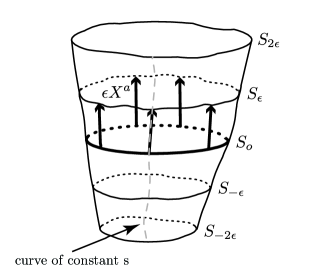
Figure 1: A schematic of a section of $\mathcal{T}_{\Phi}$ around $S_{o}$. The variation vector field $X^{a}$ is everywhere tangent to the tube, points along curves of constant $s$, and generates the foliation. Thus for sufficiently small $\epsilon$, one can intuitively write $S_{\epsilon}=S_{o}+\epsilon X$.

A variation or deformation of a two-surface $S_{o}$ is a smooth, one-to-one function $\Phi(s,\lambda):S_{o}\times[-\lambda_{o},\lambda_{o}]\rightarrow M$ (with $\lambda_{o}$ some real number) such that $\Phi(S_{o},0)=S_{o}$. Thus, $\Phi$ generates a (finite) three-surface $\mathcal{T}_{\Phi}$ and that surface is foliated by images $S_{\lambda}=\Phi(S_{o},\lambda)$ of $S_{o}$ as depicted in Fig. 1. The variation vector field $X^{a}=(\partial/\partial\lambda)^{a}$ is tangent to the curves of constant $s\in S_{o}$. The flow generated by this vector field maps leaves of constant $\lambda$ into each other. Unless otherwise noted, we will restrict our attention to normal variations where $X^{a}$ is everywhere perpendicular to the $S_{\lambda}$ and so can be written:

$$X^{a}=A\ell^{a}-Bn^{a}\,,$$ (15)

for some functions $A$ and $B$. There are no restrictions on the values of $A$ and $B$. However, in later sections we will usually assume that $X^{a}$ is $\ell$-oriented so that $A>0$. Then if $B>0$, $X^{a}$ is spacelike while $B<0$ means that it is timelike. We will mainly be interested in situations where $B>0$, hence the negative sign in (15). Fig. 2 should help to keep the various cases straight.

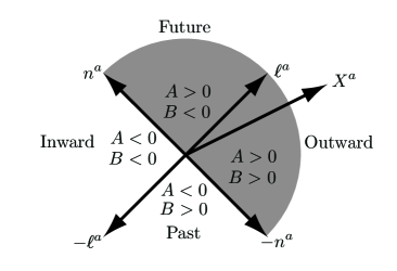
Figure 2: The normal space at a point $s\in S_{\lambda}$. Normal vectors written as $X^{a}=A\ell^{a}-Bn^{a}$ point into the causal future if $A\geq 0$ and $B\leq 0$. The shaded region represents the $\ell$-oriented vector fields for which $A>0$ and $B$ may take any value.

For any values of $A$ and $B$, the map $\Phi$ deforms $S_{o}$ into successive surfaces $S_{\lambda}$. To quantify the change in the geometry, we identify points along the curves of constant $s$ and then calculate derivatives of the intrinsic and extrinsic geometry with respect to the parameter $\lambda$. Taking the normal connection $\tilde{\omega}_{a}$ as an example, we write its variation as $\delta_{X}\tilde{\omega}_{a}$ and note that calculating this quantity amounts to:

1. using $\Phi$ to construct the $S_{\lambda}$ in a neighbourhood of $\lambda=0$,

2. constructing the $\tilde{\omega}_{a}$ on those $S_{\lambda}$ (among other things this will involve choosing a scaling of the null vectors), and

3. calculating the Lie derivative ${\cal L}\,_{X}\tilde{\omega}_{a}$ and pulling-back the result onto $S_{o}$.

Thus, once the two-surfaces are constructed and $\tilde{\omega}_{a}$ calculated, we have

$$\delta_{X}\tilde{\omega}_{a}=\tilde{q}_{a}^{c}{\cal L}\,_{X}\tilde{\omega}_{c}\,,$$ (16)

in standard four-dimensional notation.

II.2.2 Calculating variations

We now calculate some of these variations for the geometric quantities that are of interest in this paper. The easiest calculation is the variation of the two-metric. A couple of lines of algebra shows

$$\delta_{X}\tilde{q}_{ab}=Ak^{(\ell)}_{ab}-Bk^{(n)}_{ab}=(A\theta_{(\ell)}-B\theta_{(n)})\tilde{q}_{ab}+2(A\sigma^{(\ell)}_{ab}-B\sigma^{(n)}_{ab})\,,$$ (17)

from which it follows that

$$\delta_{X}\widetilde{\mbox{\boldmath$\epsilon$}}=(A\theta_{(\ell)}-B\theta_{(n)})\widetilde{\mbox{\boldmath$\epsilon$}}\,.$$ (18)

These expressions justify referring to $\theta_{(\ell)}$ and $\theta_{(n)}$ as expansions and $\sigma^{(\ell)}_{ab}$ and $\sigma^{(n)}_{ab}$ as shears; respectively they describe how $S_{o}$ expands and shears if deformed in the null directions.

Finding the variations of the extrinsic quantities is more involved. Here we just outline the calculations but more details can be found in Appendix A.2. First we note that since $\ell_{a}$ and $n_{a}$ are everywhere normal to the $S_{\lambda}$, both $\delta_{X}\ell_{a}=0$ and $\delta_{X}n_{a}=0$ (with the usual pull-backs understood). Thus

$$X^{b}\nabla_{b}\ell_{a} = -({d}_{a}-\tilde{\omega}_{a})B+\kappa_{X}\ell_{a}\,\mbox{ and}$$ (19)

$$X^{b}\nabla_{b}n_{a} = ({d}_{a}+\tilde{\omega}_{a})A-\kappa_{X}n_{a}\,\,$$ (20)

where

$$\kappa_{X}=-X^{a}n_{b}\nabla_{a}\ell^{b}\,$$ (21)

is the component of the connection on the $S_{\lambda}$ normal bundles in the $X$-direction. Explicitly, under rescalings $\ell\rightarrow f\ell$ and $n\rightarrow n/f$,

$$\kappa_{X}\rightarrow\kappa_{X}+{\cal L}\,_{X}\ln f\,\,.$$ (22)

We will usually refer to $\kappa_{X}$ as the surface gravity associated with $X^{a}$ in analogy with the corresponding quantities on a Killing or isolated horizon (though at this stage we make no claims about the physical content of this nomenclature).

The importance of (19) and (20) is that they allow us to convert expressions involving derivatives off of $S_{o}$ into ones containing only quantities defined on $S_{o}$ plus the gauge dependent surface gravity $\kappa_{X}$. Then, with the help of these relations a direct calculation shows that

$$\delta_{X}\theta_{(\ell)}-\kappa_{X}\theta_{(\ell)} = -{d}^{\,2}\mspace{-2.0mu}B+2\tilde{\omega}^{a}{d}_{a}B-B\left[|\mspace{-2.0mu}|\tilde{\omega}|\mspace{-2.0mu}|^{2}-{d}_{a}\tilde{\omega}^{a}-\tilde{R}/2+G_{ab}\ell^{a}n^{b}-\theta_{(\ell)}\theta_{(n)}\right]$$ (23)

$$\quad-A\left[|\mspace{-2.0mu}|\sigma^{(\ell)}|\mspace{-2.0mu}|^{2}+G_{ab}\ell^{a}\ell^{b}+(1/2)\theta_{(\ell)}^{2}\right]\,\,,$$

where $|\mspace{-2.0mu}|\tilde{\omega}|\mspace{-2.0mu}|^{2}=\tilde{\omega}_{a}\tilde{\omega}^{a}$ and $|\mspace{-2.0mu}|\sigma^{(\ell)}|\mspace{-2.0mu}|^{2}=\sigma^{(\ell)}_{ab}\sigma^{(\ell)ab}$.

We will also need to know $\delta_{X}\theta_{(n)}$ and this is most easily calculated by substitutions into the above expression (23). Exchanging $\ell_{a}$ and $n_{a}$ and sending $A\rightarrow-B$ and $B\rightarrow-A$ it is straightforward to see that

$$\delta_{X}\theta_{(n)}+\kappa_{X}\theta_{(n)} = {d}^{\,2}\mspace{-2.0mu}A+2\tilde{\omega}^{a}{d}_{a}A+A\left[|\mspace{-2.0mu}|\tilde{\omega}|\mspace{-2.0mu}|^{2}+{d}_{a}\tilde{\omega}^{a}-\tilde{R}/2+G_{ab}n^{a}\ell^{b}-\theta_{(\ell)}\theta_{(n)}\right]$$ (24)

$$\quad+B\left[|\mspace{-2.0mu}|\sigma^{(n)}|\mspace{-2.0mu}|^{2}+G_{ab}n^{a}n^{b}+(1/2)\theta_{(n)}^{2}\right]\,\,.$$

Finally, the variation of the normal connection (also derived in Appendix A.2) is

$$\delta_{X}\tilde{\omega}_{a}-{d}_{a}\kappa_{X} = -k^{(\ell)}_{ab}\left[{d}^{b}A+\tilde{\omega}^{b}A\right]-k^{(n)}_{ab}\left[{d}^{b}B-\tilde{\omega}^{b}B\right]$$

$$+\tilde{q}_{a}^{\;\;b}\left[\frac{1}{2}G_{bc}\tau^{c}-C_{bcde}{X}^{c}\ell^{d}n^{e}\right]\,,$$

where $\tau^{c}=A\ell^{c}+Bn^{c}$ is normal to $X^{c}$. Enlisting the help of the Codazzi equations by combining $A\times(\ref{expl2deriv})+B\times(\ref{expn2deriv})-2\times(\ref{omegaderiv})$ this can be rewritten as

$$\delta_{X}\tilde{\omega}_{a}+(A\theta_{(\ell)}-B\theta_{(n)})\tilde{\omega}_{a} = {d}_{a}\kappa_{X}-{d}_{b}\left(A\sigma_{(\ell)\;a}^{\;\;b}+B\sigma_{(n)\;a}^{\;\;b}\right)+\tilde{q}_{a}^{\;b}G_{bc}\tau^{c}$$

$$\quad+\frac{1}{2}{d}_{a}\left(A\theta_{(\ell)}+B\theta_{(n)}\right)-\theta_{(\ell)}{d}_{a}A-\theta_{(n)}{d}_{a}B\,,$$

which eliminates the Weyl dependence. This is the form that we will use.

These variations will be sufficient for most of our considerations. Note that equivalent or closely related versions of the expressions for $\delta_{X}\theta_{(\ell)}$, $\delta_{X}\theta_{(n)}$, and $\delta_{X}\tilde{\omega}_{a}$ have previously appeared in, for example, GourgFlux ; MK ; ams ; eardley ; meRev ; HaywardDualNull , though not with the particular two-surface emphasis that we adopt here.

II.3 Angular momentum and its evolution

Physically, the connection $\tilde{\omega}_{a}$ defines the angular momentum associated with any rotation vector field $\phi^{a}$ on a closed two-surface $S$ by ; ak ; prl ; GourgFlux ; KrishNum ; haywardFlux . By definition the flow associated with such a $\phi^{a}$ has only two fixed points and foliates the remainder of $S$ into closed integral curves of parameter length $2\pi$. The canonical example of such a field is a Killing vector field of the two-metric $\tilde{q}_{ab}$ and in that particular case it replaces the flat-space notion of an axis of rotation. However even if it is not a Killing vector field, it is standard to define the angular momentum of $S$ relative to $\phi^{a}$ as

$$J[\phi]=\frac{1}{8\pi G}\int_{S}\widetilde{\mbox{\boldmath$\epsilon$}}\phi^{a}\tilde{\omega}_{a}\,\,.$$ (27)

Note that any rotation vector field $\phi^{a}$ is necessarily divergence free and a quick calculation with the help of (9) shows that this expression is independent of the scaling of the null vector fields. Alternatively if the surface $S$ has a suitable topology such as $S^{2}$, then a divergence free $\phi^{a}$ can necessarily be written in the form $\phi^{a}=\tilde{\epsilon}^{ab}d_{b}\zeta$ for the area-form $\tilde{\epsilon}_{ab}$ and some function $\zeta$. Then, the scaling independence is made explicit if we rewrite (27) as

$$J[\phi]=\frac{1}{8\pi G}\int_{S}\mspace{-6.0mu}\zeta\mathbf{\Omega}\,,$$ (28)

where as usual we drop the indices and write in bold any form that is being integrated over.

We now consider how the angular momentum changes under deformations. To this end we multiply (II.2.2) by the area form $\widetilde{\mbox{\boldmath$\epsilon$}}$ and so obtain

$$\delta_{X}\left(\widetilde{\mbox{\boldmath$\epsilon$}}\tilde{\omega}_{a}\right) = \widetilde{\mbox{\boldmath$\epsilon$}}\left({d}_{a}\kappa_{X}-{d}_{b}\left(A\sigma^{(\ell)b}_{a}+B\sigma^{(n)b}_{\;a}\right)+\tilde{q}_{a}^{\;b}G_{bc}\tau^{c}\right)$$

$$\qquad+\widetilde{\mbox{\boldmath$\epsilon$}}\left(\frac{1}{2}{d}_{a}\left(A\theta_{(\ell)}+B\theta_{(n)}\right)-\theta_{(\ell)}{d}_{a}A-\theta_{(n)}{d}_{a}B\right)\,.$$

Now, extend $\phi^{a}$ off of $S$ by demanding that $\delta_{X}\phi^{a}=0$ — essentially this is equivalent to the flat space requirement that angular momentum be measured relative to a fixed axis of rotation. Then, contracting (II.3) with $\phi^{a}$ and integrating over $S$, several total divergence terms vanish and we find that

$$\delta_{X}J[\phi]=\frac{1}{8\pi G}\int_{S}\widetilde{\mbox{\boldmath$\epsilon$}}\left\{G_{ab}\phi^{a}\tau^{b}+\sigma^{({\tau})}\mspace{-6.0mu}:\mspace{-4.0mu}\sigma^{(\phi)}+A\phi^{a}d_{a}\theta_{(\ell)}+B\phi^{a}d_{a}\theta_{(n)}\right\}\,,$$ (30)

where the shear with respect to a general vector field $w^{a}$ is

$$\sigma_{ab}^{(w)}\equiv\left(\tilde{q}_{a}^{c}\tilde{q}_{b}^{d}-\frac{1}{2}\tilde{q}_{ab}\tilde{q}^{cd}\right)\nabla_{c}w_{d}\,,$$ (31)

and $\sigma^{({\tau})}\mspace{-6.0mu}:\mspace{-4.0mu}\sigma^{(\phi)}=\sigma^{(\tau)}_{ab}\sigma^{(\phi)ab}$ (this double contraction notation is adopted from GourgFlux ).

We will return to equation (30) in SectionV.3 where we will be able to neglect the last two-terms and so interpret the change in angular momentum as coming from a flux of stress-energy (with the help of the Einstein equation) and a flux of shear. A detailed discussion and fluid mechanical interpretation of (II.3) and (30) can also be found in GourgFlux .

II.4 The “constraint” law

Finally, before specializing to the two-surfaces associated with horizons we derive the following relation. First, combining $A\times(\ref{explderiv})+B\times(\ref{expnderiv})$ we find that

$$\kappa_{X}\theta_{X} = A\delta_{X}\theta_{(\ell)}+B\delta_{X}\theta_{(n)}+d_{a}(Ad^{a}B-Bd^{a}A-2AB\tilde{\omega}^{a})$$

$$+\sigma^{(\tau)}\mspace{-6.0mu}:\mspace{-4.0mu}\sigma^{(X)}+G_{ab}X^{a}\tau^{b}+\frac{1}{2}\theta_{(X)}\theta_{(\tau)}\,,$$

where we again have $\tau_{a}=A\ell_{a}+Bn_{a}$ and $\theta_{(X)}$ and $\theta_{(\tau)}$ are defined in the obvious way. Integrating this over $S$, the total divergence term vanishes and we find that

$$\frac{1}{8\pi G}\int_{S}\kappa_{X}\delta_{X}\tilde{\epsilon} = \frac{1}{8\pi G}\int_{S}\tilde{\epsilon}\left[G_{ab}X^{a}\tau^{b}+\sigma^{(X)}\mspace{-6.0mu}:\mspace{-4.0mu}\sigma^{(\mathcal{\tau})}\right]$$ (33)

$$\qquad+\frac{1}{8\pi G}\int_{S}\tilde{\epsilon}\left[A\delta_{X}\theta_{(\ell)}+B\delta_{X}\theta_{(n)}+\frac{1}{2}\theta_{(X)}\theta_{(\mathcal{\tau})}\right]\,.$$

More generally for a vector field

$$\mathcal{X}^{a}=X^{a}+\tilde{x}^{a}\,,$$ (34)

where $\tilde{x}^{a}$ is everywhere transverse to the $S$ we can combine (II.3) and (II.4) to obtain

$$\frac{1}{8\pi G}\int_{S}\left\{\kappa_{X}\delta_{X}\widetilde{\mbox{\boldmath$\epsilon$}}+\tilde{x}^{a}\delta_{X}\left(\tilde{\epsilon}\tilde{\omega}_{a}\right)\right\} = \frac{1}{8\pi G}\int_{S}\tilde{\epsilon}\left[G_{ab}\mathcal{X}^{a}\tau^{b}+\sigma^{(\mathcal{X})}\mspace{-6.0mu}:\mspace{-4.0mu}\sigma^{(\mathcal{\tau})}\right]$$

$$\qquad+\frac{1}{8\pi G}\int_{S}\tilde{\epsilon}\left[A\delta_{\mathcal{X}}\theta_{(\ell)}+B\delta_{\mathcal{X}}\theta_{(n)}+\frac{1}{2}\theta_{(X)}\theta_{(\mathcal{\tau})}\right]\,.$$

In cases where $\kappa_{X}$ is constant and $\tilde{x}^{a}=\Omega\phi^{a}$ for some constant $\Omega$ (which is not related to the curvature of the normal bundle) and rotation vector field satisfying $\delta_{X}\phi^{a}=0$, the left-hand side of this equation takes a particularly familiar form:

$$\frac{\kappa_{X}}{8\pi G}\dot{a}+\Omega\dot{J}[\phi]\,\,.$$ (36)

The similarity to the first law of black hole mechanics is not coincidence. In sections V and VI we will see that the dynamical version of the first law for both event and trapping horizon are closely related to (II.4).

A version of this relation was referred to as the horizon constraint law in prl ; theBeast due to its equivalence to the integrated diffeomorphism constraint on $\mathcal{T}_{\Phi}$. A discussion of its terms and their interpretation if the horizon is viewed as a viscous fluid can also be found in GourgFlux . Furthermore, in Gourgoulhon:2006uc , equation (II.4) is interpreted as a second order evolution equation for the area.

III Future outer trapped surfaces

The expressions of the previous section hold for any spacelike two-surface embedded in any four-dimensional spacetime. In this paper however, our main interest will in the two-surfaces that foliate future outer trapping horizons which in turn are embedded in solutions of the Einstein equations. Thus in this section we consider spacelike two-surfaces on which $G_{ab}=8\pi T_{ab}$ and for which $\theta_{(\ell)}=0$, $\theta_{(n)}<0$ and there is a scaling of the null vectors such that $\delta_{n}\theta_{(\ell)}<0$. Adapting Hayward’s nomenclature we will call such surfaces future outer trapping surfaces (FOTS).

First, we consider the conditions under which a marginally trapped surface $S$ with $\theta_{(\ell)}=0$ and $\theta_{(n)}<0$ is a FOTS. To this end, we we set $A=0$, $B=-1$ and $\theta_{(\ell)}=0$ in (23) and so find that on a marginally trapped surface

$$\delta_{n}\theta_{(\ell)}=-\tilde{R}/2+|\mspace{-2.0mu}|\tilde{\omega}|\mspace{-2.0mu}|^{2}-{d}_{a}\tilde{\omega}^{a}+(8\pi G)T_{ab}\ell^{a}n^{b}\,.$$ (37)

Then it is immediate that the $\delta_{n}\theta_{(\ell)}<0$ condition is determined entirely by this component of the stress-energy tensor along with the intrinsic and extrinsic geometry of $S$ – no derivatives need to be taken off of the surface. That said, checking this condition is slightly more complicated than just calculating this quantity with an arbitrary scaling of the null vectors. For example, in Appendix C it is shown that for the standard scaling of null vectors on a Kerr horizon, $\delta_{n}\theta_{(\ell)}$ is not always less then zero. A rescaling is necessary for this relationship to become apparent.

Now, for any spacelike two-surface on which $\theta_{(\ell)}=0$, equation (23) simplifies to become

$$\delta_{X}\theta_{(\ell)}=-{d}^{\,2}\mspace{-2.0mu}B+2\tilde{\omega}^{a}{d}_{a}B-B\delta_{n}\theta_{(\ell)}+A\delta_{\ell}\theta_{(\ell)}\,,$$ (38)

where $\delta_{n}\theta_{(\ell)}$ takes the form shown in equation (37) and

$$\delta_{\ell}\theta_{(\ell)} = -|\mspace{-2.0mu}|\sigma^{(\ell)}|\mspace{-2.0mu}|^{2}-(8\pi G)T_{ab}\ell^{a}\ell^{b}\,\,.$$ (39)

If this is a FOTS we can adopt a scaling so that $\delta_{n}\theta_{(\ell)}<0$, while if we assume the null energy condition it also follows that $\delta_{\ell}\theta_{(\ell)}\leq 0$. Then, we can draw several conclusions about FOTS.

First strengthening to the dominant energy condition, there is the well-known newman restriction on the topology of such a surface.

FOTS Property 1

If $S$ is a closed and orientable FOTS on which the dominant energy condition holds, then it is homeomorphic to $S^{2}$.

This follows from equation (37). On integrating this over $S$ and doing a bit of rearranging we find that :

$$\chi=\frac{1}{2\pi}\int_{S}\tilde{\epsilon}\left\{-\delta_{n}\theta_{(\ell)}+|\mspace{-2.0mu}|\tilde{\omega}|\mspace{-2.0mu}|^{2}+8\pi T_{ab}\ell^{a}n^{b}\right\}\,,$$ (40)

where $\chi$ is the Euler characteristic of $S$. Now, by assumption $\delta_{n}\theta_{(\ell)}<0$ while the dominant energy condition implies that the matter term is positive. Thus $\chi>0$ and this is sufficient to tell us that $S$ must be homeomorphic to a two-sphere since that is the only closed and orientable two-surface with positive Euler characteristic. $\Box$

Next, we consider the conditions under which a FOTS may be deformed whilst preserving its defining characteristics. Sufficiently small variations will always leave $\theta_{(n)}<0$ and $\delta_{n}\theta_{(\ell)}<0$ and so the key to understanding these deformations is finding normal vector fields $X^{a}$ such that $\delta_{X}\theta_{(\ell)}=0$. We assume that all fields are at least twice differentiable.

We begin with the case where $\delta_{\ell}\theta_{(\ell)}=0$ everywhere on a FOTS. Then we have:

FOTS Property 2

If $S$ is a FOTS on which $\delta_{\ell}\theta_{(\ell)}=0$ everywhere, then variation vectors $X^{a}$ satisfy $\delta_{X}\theta_{(\ell)}=0$ if and only if they are parallel to $\ell^{a}$.

Starting with the first part, if $\delta_{\ell}\theta_{(\ell)}=0$ everywhere on $S$ then equation (38) becomes

$$\delta_{X}\theta_{(\ell)}={d}^{\,2}\mspace{-2.0mu}B-2\tilde{\omega}^{a}{d}_{a}B+B\delta_{n}\theta_{(\ell)}\,\,,$$ (41)

and it is trivial that $B=0\Rightarrow\delta_{X}\theta_{(\ell)}=0$ for any value of $A$. It is also straightforward to see that the converse must be true. First applying the maximum principle of Appendix B to $\delta_{X}\theta_{(\ell)}=0$ we find that $B$ must be either constant or everywhere negative. Similarly applying the corresponding minimum principle to $-\delta_{X}\theta_{(\ell)}=0$ we find that $B$ must be either constant or everywhere positive. Thus, $B$ must be constant and it is clear that since $\delta_{n}\theta_{(\ell)}\neq 0$ that constant must be zero. The result is established. $\Box$

It is also true that all such deformations leave the intrinsic geometry of $S$ invariant:

FOTS Property 3

Let $S$ be a FOTS on which $\delta_{\ell}\theta_{(\ell)}=0$ everywhere and the null energy condition holds. Then $\delta_{X}\theta_{(\ell)}=0$ implies that $\delta_{X}\tilde{q}_{ab}=0$. That is, all deformations leave the intrinsic geometry invariant.

If the null energy condition holds then all terms in (39) are non-negative and so if $\delta_{\ell}\theta_{(\ell)}=0$ they must all, including $\sigma^{(\ell)}_{ab}$, be zero. Then with $B=0$ by Property 2 and $\theta_{(\ell)}=0$ by assumption, equation (17) implies that $\delta_{X}\tilde{q}_{ab}=0$ as required. $\Box$

Such results are familiar from the isolated horizon literature and we will return to them in section IV. For now however we consider FOTS on which $\delta_{\ell}\theta_{(\ell)}$ is somewhere non-zero. In doing this we restrict our attention to $\ell$-oriented variation vector fields for which $A>0$ (Fig. 2).

FOTS Property 4

Let $S$ be a FOTS and assume the null energy condition. Then, if $\delta_{\ell}\theta_{(\ell)}\neq 0$ anywhere on $S$, all $\ell$-oriented variation vectors $X^{a}$ that satisfy $\delta_{X}\theta_{(\ell)}=0$ are spacelike everywhere on $S$.

If the null energy condition holds then $\delta_{\ell}\theta_{(\ell)}\leq 0$ by equation (39). Thus with $A>0$, equation (38) implies that

$$-{d}^{\,2}\mspace{-2.0mu}B+2\tilde{\omega}^{a}{d}_{a}B-B\delta_{n}\theta_{(\ell)}\geq 0\,,$$ (42)

everywhere on $S$. Then by the minimum principle of Appendix B, $B$ is either everywhere positive or everywhere constant. If it is constant then the derivatives in (38) vanish and

$$B=A\left(\frac{\delta_{\ell}\theta_{(\ell)}}{\delta_{n}\theta_{(\ell)}}\right)\,.$$ (43)

everywhere on $S$. In particular this must hold at the point where $\delta_{\ell}\theta_{(\ell)}<0$ and so with $A>0$ and $\delta_{n}\theta_{(\ell)}<0$ we again find that $B>0$. Thus in either case $g_{ab}X^{a}X^{b}=2AB>0$ and $X^{a}$ is spacelike. $\Box$

Combining this with Property 2 we see that FOTS satisfying the null energy condition may be cleanly split into two classes – those for which $\ell$-oriented variation vector fields satisfying $\delta_{X}\theta_{(\ell)}=0$ are null and those for which these vectors are spacelike. Such an $X^{a}$ cannot be timelike and what is more it cannot be partly null and partly spacelike.

We also know something about how the geometry of a FOTS must change with respect to a spacelike $\theta_{(\ell)}=0$ preserving deformation:

FOTS Property 5

Let $S$ be a FOTS and assume the null energy condition. Then if $\delta_{\ell}\theta_{(\ell)}$ is non-zero anywhere on $S$, $\delta_{X}\widetilde{\mbox{\boldmath$\epsilon$}}>0$ everywhere. The deformation causes $S$ to expand everywhere.

If $\delta_{\ell}\theta_{(\ell)}\neq 0$ anywhere on $S$, then by Property 4, $X^{a}$ must be everywhere spacelike with $B>0$. Then $\delta_{X}\widetilde{\mbox{\boldmath$\epsilon$}}=-B\theta_{(n)}\widetilde{\mbox{\boldmath$\epsilon$}}$ where $-B\theta_{(n)}>0$ since $\theta_{(n)}<0$ by assumption. $\Box$

Finally, it is quite clear that in general there will be an infinite number of $X^{a}$ that will solve $\delta_{X}\theta_{(\ell)}=0$ and so an equally infinite number of FOTS-preserving deformations. For example, if $\delta_{\ell}\theta_{(\ell)}$ is nowhere zero and we choose any $B\in C^{2}(S)$ then we can always solve $\delta_{X}\theta_{(\ell)}=0$ to find a corresponding $A$ (though unless $B$ is constant, there is no guarantee that the resulting $X^{a}$ will be $\ell$-oriented). Furthermore if $\delta_{\ell}\theta_{(\ell)}=0$ everywhere, then Property 2 tells us that for any $X^{a}=A\ell^{a}$, $\delta_{X}\theta_{(\ell)}=0$.

In contrast to the $\delta_{\ell}\theta_{(\ell)}=0$ case where all allowed variation vector fields must be parallel to $\ell^{a}$, if $\delta_{\ell}\theta_{(\ell)}$ is somewhere non-zero then (apart from constant rescalings) no two variation vector fields are parallel. Instead they must interweave as shown in Fig. 3.

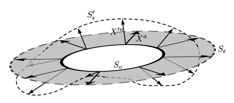
Figure 3: Given two spacelike variation vector fields $X^{a}$ and $X^{\prime a}$ on a FOTS that satisfy $\delta_{X}\theta_{(\ell)}=\delta_{X^{\prime}}\theta_{(\ell)}=0$, then if they are not constant multiples of each other they must interweave so that $X^{\prime a}$ will sometimes point into the future of $X^{a}$ and sometimes will point into the past.

FOTS Property 6

Let $S$ be a FOTS with $\delta_{\ell}\theta_{(\ell)}$ somewhere non-zero and assume the null energy condition. Further let $X^{a}$ and $X^{\prime a}$ be two $\ell$-oriented, FOTS-preserving deformation vector fields. Then either

1. $X^{\prime a}=\lambda_{o}X^{a}$ for some constant $\lambda_{o}$ or

2. $X^{\prime a}$ interweaves $X^{a}$ in the sense that $X^{\prime a}\tau_{a}$ takes both positive and negative values on $S$, where $\tau^{a}=A\ell^{a}+Bn^{a}$ is the usual forward pointing timelike normal to $S$.

By Property 4, both $X^{a}$ and $X^{\prime a}$ are spacelike and so with $X^{a}=A\ell^{a}-Bn^{a}$ for some positive $A$ and $B$, we have

$$X^{\prime a}=(\alpha+\lambda)A\ell^{a}-\lambda Bn^{a}$$ (44)

for some functions $\alpha$ and $\lambda$ that satisfy both $\lambda>0$ and $\alpha+\lambda>0$.

Now, to begin our analysis, let us consider the case where $\alpha$ takes both positive and negative values. Then we immediately see that

$$X^{\prime a}\tau_{a}=-\alpha AB\,,$$ (45)

and so this corresponds to the second posited behaviour for $X^{\prime a}$.

By contrast, if $\alpha$ does not take both positive and negative values then at least one of $\alpha\leq 0$ or $\alpha\geq 0$ must be true. As preparation to exploring these two possibilities, we note that given $\delta_{X}\theta_{(\ell)}=0$, it is straightforward to see that $\delta_{X^{\prime}}\theta_{(\ell)}=0$ reduces to

$$Bd^{2}\lambda+2({d}^{a}B-B\tilde{\omega}^{a}){d}_{a}\lambda=\alpha A\delta_{\ell}\theta_{(\ell)}\,\,.$$ (46)

Thus, if $\alpha\leq 0$ this equation implies that

$$Bd^{2}\lambda+2({d}^{a}B-B\tilde{\omega}^{a}){d}_{a}\lambda\geq 0\,.$$ (47)

Now, $\lambda$ must achieve a maximum on $S$, so we can define a new function $\lambda^{\star}=\lambda-\lambda_{max}$ that also satisfies equation (47) and achieves a maximum value of zero. Then, by our usual maximum principle, since $\lambda^{\star}$ is not everywhere negative, it must be constant. This means that $\lambda$ is also constant and so by (46), $\alpha=0$. Thus $\alpha\leq 0\Rightarrow X^{\prime a}=\lambda_{o}X^{a}$ for some constant $\lambda_{o}$. Similar reasoning shows that $\alpha\geq 0$ also implies that $X^{\prime a}$ is a constant multiple of $X^{a}$. $\Box$

IV Horizons and their properties

In this section we apply the properties of FOTS to gain a better understanding of future outer trapping horizons. First though we recall some definitions.

IV.1 Horizons

We begin with the definition of a future outer trapping horizon (FOTH). A trapping horizon is a three-dimensional submanifold of a spacetime $(M,g_{ab})$ that may be foliated with closed and spacelike two-surfaces $S_{v}$ (where $v$ is a foliation parameter) on which $\theta_{(\ell)}=0$ hayward . Trapping horizons are classified by the values taken by $\theta_{(n)}$ and $\delta_{n}\theta_{(\ell)}$ on their leaves. A trapping horizon is said to be future (past) if $\theta_{(n)}<0$ ($\theta_{(n)}>0$) while it is outer (inner) if there is a scaling of the null vectors such that $\delta_{n}\theta_{(\ell)}<0$ ($\delta_{n}\theta_{(\ell)}>0$). These names are taken from the horizons that satisfy these conditions in a fully extended Kerr or Reissner-Nordström spacetime. Thus the event horizon is a future outer trapping horizon (FOTH) and the inner Cauchy horizon is future inner. The corresponding white hole horizons are past outer and past inner respectively. In this paper, we will be mainly in interested in FOTHs (which are foliated by FOTS).

As noted in the introduction, apart from (future outer) trapping horizons, there are other closely related quasilocal horizons. Here we recall the definition of isolated and dynamical horizons, while in section V we will consider slowly evolving horizons.

A three-dimensional submanifold of a spacetime $(M,g_{ab})$ is a non-expanding horizon if: i) it is null and topologically $S\times{\mbox{\rm$\mbox{I}\!\mbox{R}$}}$ for some closed two-manifold $S$, ii) $\theta_{(\ell)}=0$ and iii) $-T^{ab}\ell_{b}$ is future directed and causal isoMech . As usual $\ell^{a}$ is an outward pointing normal and we note that since the horizon is null, no foliation is required for its construction. However, a foliation is certainly no hindrance to a three-surface being a non-expanding horizon, and any null FOTH satisfying the null energy condition will certainly be a non-expanding horizon.

Non-expanding horizons are the simplest objects in the isolated horizon family. Any non-expanding horizon can be turned into a weakly isolated horizon if the scaling of the null vectors is chosen so that ${\cal L}\,_{\ell}\omega_{a}=0$ for

$$\omega_{a}:=-n_{b}\nabla_{\underleftarrow{a}}\ell^{b}=-\kappa_{\ell}n_{a}+\tilde{\omega}_{a}\,,$$ (48)

where the arrow indicates a pull-back into the cotangent bundle of the non-expanding horizon. With this scaling zeroth and first laws of isolated horizon mechanics may be established isoMech . Furthermore, an isolated horizon is obtained by strengthening the above conditions to require that the entire extrinsic geometry encoded in the derivative operator be time independent.

Finally, a three-dimensional sub-manifold of a spacetime $(M,g_{ab})$ is a dynamical horizon if it: i) is spacelike and ii) can be foliated by spacelike two-surfaces such that the null normals to those surfaces satisfy $\theta_{(\ell)}=0$ and $\theta_{(n)}<0$ ak . As we shall see in the next subsection, if the null energy condition holds and $\delta_{\ell}\theta_{(\ell)}\neq 0$ then dynamical horizons are FOTHs and vice versa.

Non-expanding, isolated and dynamical horizons each have a rich set of properties that may be derived directly from their definitions. However, examples of spacetimes exist that contain (and are actually foliated by) isolated horizons but do not contain trapped surfaces LewIso . Similarly there are spacetimes with dynamical horizons but no trapped surfaces pp . Thus if we take trapped surfaces as the defining property of black holes, neither of these definitions is sufficient to specifically single out black holes. Instead they represent necessary conditions which must be supplemented to become sufficient.

Given this observation, we will take FOTHs as our basic objects and classify them by hybridizing the naming systems. Thus a FOTH that also satisfies one of these other sets of properties will be referred to as non-expanding, weakly isolated, or dynamical as appropriate.

IV.2 Properties of FOTHs

A FOTH can be thought of as the variation surface associated with a (finite) deformation of a FOTS (like the one shown in Fig. 1). Specifically given a FOTH and a foliation labelling $v$, we can always find a tangent vector field $\mathcal{V}$ that is normal to the $S_{v}$ and which satisfies

$${\cal L}\,_{\mathcal{V}}v=1\,\,.$$ (49)

Then, $\mathcal{V}^{a}$ can be viewed as a variation vector field and as for other deformation vectors we write

$$\mathcal{V}^{a}=A\ell^{a}-Bn^{a}\,,$$ (50)

for some functions $A$ and $B$. Further, identifying points on the different $S_{v}$ by the flow generated by $\mathcal{V}$, we write derivatives of the two-geometry with respect to $v$ as

$$\frac{d}{dv}\equiv\delta_{\mathcal{V}}\,\,.$$ (51)

Then we may apply our results on FOTS to learn about FOTHs.

First, their topology is strongly constrained hayward and this follows directly from FOTS Property 1:

FOTH Property 1

Let $H$ be a FOTH and assume the dominant energy condition. Then $H$ has topology $S^{2}\times{\mbox{\rm$\mbox{I}\!\mbox{R}$}}$.

Next, we consider the circumstances under which a FOTH is non- expanding and those by which it is dynamical. In particular we will be interested in transitions between these behaviours and so as a preliminary we define non-expanding and dynamical sections of a FOTH. If a FOTH $H$ is null (that is $B=0$ everywhere) for some range $v_{1}\leq v\leq v_{2}$ of the foliation parameter then we will refer to this as a non-expanding section of $H$. In contrast if $H$ is spacelike (that is $AB>0$ everywhere) for some range $v^{\prime}_{1}<v<v^{\prime}_{2}$ of the foliation parameter then we will refer to this as a dynamical section of $H$.

Then by FOTS Properties 2 and 4, on any $S_{v}$ of a FOTH either $B=0$ everywhere or $B\neq 0$ anywhere. Thus, no element of the foliation is partly non-expanding and partly dynamical. Transitions between non-expanding and dynamical sections must happen “all-at-once”.

FOTH Property 2

Let $H$ be a FOTH with foliation $S_{v}$ and assume the null energy condition. Then $H$ may be completely partitioned into non-expanding and dynamical sections. On non-expanding sections $\delta_{\ell}\theta_{(\ell)}=0$ everywhere while on dynamical sections $\delta_{\ell}\theta_{(\ell)}<0$ at least somewhere on each $S_{v}$.

This surprising result was first shown (using slightly different assumptions) in ams . As one application, it guarantees that a FOTH on which $\delta_{\ell}\theta_{(\ell)}\neq 0$ for at least one point on each cross section is necessarily a dynamical horizon. The converse is slightly more restricted and we must require that $\delta_{\ell}\theta_{(\ell)}\neq 0$ everywhere to ensure that a dynamical horizon also be a FOTH. To see this consider that a dynamical horizon is necessarily spacelike and so $X^{a}$ can always be oriented so that $A>0$ and $B>0$. Scaling the null vectors so that $B$ is constant on each cross-section of the horizon (38) simplifies to

$$B\delta_{n}\theta_{(\ell)}=A\delta_{\ell}\theta_{(\ell)}\,\,.$$ (52)

Thus, if $\delta_{\ell}\theta_{(\ell)}\neq 0$ everywhere on a cross-section then the null energy condition guarantees that is strictly negative and so $\delta_{n}\theta_{(\ell)}<0$ everywhere as well. Consequently such a dynamical horizon is a FOTH. However, if $\delta_{\ell}\theta_{(\ell)}=0$ somewhere (or everywhere) on the surface, then at those points $\delta_{n}\theta_{(\ell)}$ will also vanish and the dynamical horizon will not be a FOTH. Examples of such dynamical horizons are considered in pp .

Next by FOTS Properties 3 and 5, dynamical versus non-expanding sections differ in more than just signature:

FOTH Property 3

Let $\Delta H$ be a (section of a) FOTH and assume that the null energy condition holds.

1. If $\Delta H$ is non-expanding, then the intrinsic geometry of the $S_{v}$ is invariant. That is $\delta_{\mathcal{V}}\tilde{q}_{ab}=0$.

2. If $\Delta H$ is dynamical, then $S_{v}$ locally increases in area everywhere. That is $\delta_{\mathcal{V}}\widetilde{\mbox{\boldmath$\epsilon$}}=F\widetilde{\mbox{\boldmath$\epsilon$}}$ for some function $F$ that is everywhere positive.

The first part of this property is well known from the isolated horizon literature isoMech ; isoGeom . The second part is essentially Hayward’s second law of black hole mechanics hayward . FOTHs expand if and only if they are dynamical. Otherwise their intrinsic geometry is unchanging.

Having reaffirmed these basic results, we can consider how FOTHs may be deformed while preserving their defining characteristics. First we consider variations of the foliation that leave $H$ itself invariant.

FOTH Property 4

Let $H$ be a FOTH and assume that the null energy condition holds.

1. If $H$ is non-expanding then the foliation may be smoothly deformed by any vector field of the form $X^{a}=f\ell^{a}$ where $f$ is any positive function.

2. If $H$ is dynamical then the foliation is rigid and can be relabelled but not deformed.

The first part of this property follows directly from FOTS Property 2 which we apply to all of the $S_{v}$ simultaneously. The second part follows from FOTS Property 6 which tells us that if $\delta_{\mathcal{V}}\theta_{(\ell)}=0$ then $\delta_{(\alpha\mathcal{V})}\theta_{(\ell)}=0$ if and only if $\alpha$ is a constant over $S_{v}$. For such a constant $\alpha$ the variation would preserve (but relabel) the foliation.

Thus, the foliation may be deformed in an infinite number of ways on a non-expanding (section of a) FOTH while it may not be deformed at all on a dynamical section. The first part of this property is consistent with the fact that particular foliations are not important for most of the isolated horizon formalism. The second part is consistent with the more general result of gregabhay which says that if $S$ is a FOTS and $H$ is a dynamical FOTH with foliation $S_{v}$, then $S\subset H$ if and only if it $S=S_{v}$ for some $v$.

Next, we consider the other ways in which a FOTH may be deformed. Again the non-expanding and dynamical cases are quite different.

FOTH Property 5

Let $H$ be a FOTH and assume the null energy condition. We consider variations that deform $H$ but preserve the FOTH conditions.

1. If $H$ is non-expanding then all allowed variations map $H$ into itself.

2. If $H$ is dynamical then all allowed variations deform each leaf of its foliation partly into the causal future and partly into the causal past of $H$.

This property also follows directly from FOTS Properties 2 and 6 and can be rephrased to say that non-expanding FOTHs are stable against deformations but dynamical FOTHs are not stable in his way. The second part is consistent with gregabhay where it was shown that if $H_{1}$ and $H_{2}$ are dynamical FOTHs with foliations $S_{v_{1}}$ and $S_{v_{2}}$ respectively, then no $S_{v_{1}}$ can lie entirely in the causal past (or future) of $H_{2}$ and vice versa. Thus, either $S_{v_{1}}$ is causally disconnected from $H_{2}$ or it intersects it so that it lies partly in the causal future and partly in the causal past. Property 5 may be thought of as a local version of that global result.

V Slowly evolving horizons and their flux laws

A significant part of physics deals with systems that are at or near equilibrium. For horizons, we naturally take non-expanding FOTHs to be equilibrium states. Included in this class are the event horizons of all (non-extreme) Kerr-Newmann black holes (whose properties are summarized in Appendix C). Further, such FOTHs are automatically isolated horizons and so all of the results from that formalism apply to them. Recall too that by FOTH Property 5, these surfaces (locally) can only be deformed into themselves, so there is no ambiguity about their exact location.

It is then natural to consider near-equilibrium horizons, which should be those that change slowly in time. Now, while this is a very reasonable condition intuitively, it is not so easy to geometrically and invariantly characterize such horizons — keep in mind that dynamical FOTHs are spacelike and so there is no natural notion of time intrinsically associated with the surface. In this section we will motivate a definition of these slowly evolving horizons and then explore some of its consequences. A version of the definition and many of the properties appeared in prl but most of the derivations appear here for the first time.

V.1 Slowly expanding horizons

Intuitively, we would expect the properties of a slowly expanding horizon to be “close” to those of a non-expanding or isolated horizon. In this section we will formalise this requirement. This is essentially done by performing a perturbation expansion around a non-expanding horizon in powers of a small parameter $\epsilon$. However, as we shall see, care must be taken as spacelike and null surfaces are fundamentally different, and in particular it is non-trivial to find a normalization which transitions smoothly between the dynamical and isolated regimes.

In order to proceed, we will slightly modify the formalism introduced over the last three sections. First we loosen it so that while the evolution vector field $\mathcal{V}^{a}$ still generates the foliation, it is no longer tied to a specific labelling; that is we only require that ${\cal L}\,_{\mathcal{V}}v=\alpha(v)$ for some positive function $\alpha(v)$. Next we tighten it by choosing $A=1$ so that

$$\mathcal{V}^{a}=\ell^{a}-Cn^{a}\,,$$ (53)

where we change notation from $B$ to $C$ to avoid confusion with the more general variations considered previously. The net effect is to reduce the scaling freedom of the null vectors to that contained in $\alpha(v)$ so that for a fixed foliation labelling

$$\mathcal{V}^{a}=\alpha\mathcal{V}_{o}^{a}\,\,,\ell^{a}=\alpha\ell_{o}^{a}\,\,,n^{a}=\frac{1}{\alpha}n_{o}^{a}\,\,\mbox{and}\,\,C=\alpha^{2}C_{o}\,,$$ (54)

where the subscript “o” indicates a quantity defined with $\alpha=1$.

If a FOTH is null and non-expanding, then $C=0$ and the evolution vector field $\mathcal{V}=\ell$. Thus, the most direct way to define a slowly expanding horizon might seem to be to say that it is a (section of) a horizon on which $C$ is very small. Unfortunately this is not a viable strategy as one can use the rescaling freedom (54) to make $C$ arbitrarily small on any $\triangle H$. Instead we proceed by focusing on how the $S_{v}$ are evolved by $\mathcal{V}^{a}$.

For our purposes non-expanding horizons have two key properties: they are null and the intrinsic geometry of their foliating two-surfaces is invariant. Our invariant characterization of a slowly expanding horizon draws on both of these ideas. First, we consider the evolution of the area-form $\widetilde{\mbox{\boldmath$\epsilon$}}$ on $S_{v}$. From (18) we have

$${\cal L}\,_{\mathcal{V}}\widetilde{\mbox{\boldmath$\epsilon$}}=-C\theta_{(n)}\widetilde{\mbox{\boldmath$\epsilon$}}\,,$$ (55)

which is certainly scaling dependent. However this dependence may be easily isolated by rewriting

$${\cal L}\,_{\mathcal{V}}\widetilde{\mbox{\boldmath$\epsilon$}}=-C\theta_{(n)}\widetilde{\mbox{\boldmath$\epsilon$}}=||\mathcal{V}||\left(-\sqrt{\frac{C}{2}}\theta_{(n)}\widetilde{\mbox{\boldmath$\epsilon$}}\right)\,,$$ (56)

so that the rescaling freedom is restricted to $||\mathcal{V}||$. The term in parentheses then provides an invariant measure of the rate of expansion. Among other properties it vanishes if the horizon is non-expanding and on a dynamical horizon section is equal to the rate expansion of $\widetilde{\mbox{\boldmath$\epsilon$}}$ with respect to the unit-normalized version of the evolution vector field. We will consider the rate of expansion to be slow if this is small and this approach is borne out by the examples of billsPaper . In particular if $-\sqrt{C}\theta_{(n)}$ is of order $\epsilon$ and the scaling of the null vectors is chosen so that $||\mathcal{V}||$ is commensurate (as would be reasonable for an “almost-null” surface) then ${\cal L}\,_{\mathcal{V}}\widetilde{\mbox{\boldmath$\epsilon$}}$ will be of order $\epsilon^{2}$.

This notion of a slow area change captures the essence of a slowly expanding horizon however we still need to require both that the surface be “almost-null” and that the rest of the intrinsic geometry also be slowly changing. We have already seen that restrictions on the norm of $\mathcal{V}^{a}$ are not invariant, so instead we will implement these ideas together by requiring that the evolution of the two-metric be characterized by the expansion and shear associated with $\ell^{a}$ (as they would be for a truly null surface). That is from (17),

$${\cal L}\,_{\mathcal{V}}\tilde{q}_{ab}=2\sigma^{(\ell)}_{ab}+\left(-C\theta_{(n)}\tilde{q}_{ab}-2C\sigma^{(n)}_{ab}\right)\approx 2\sigma^{(\ell)}_{ab}\,.\\$$

Further, the matter flow across the horizon similarly should be, to lowest order, the same as that across a null surface. That is we expect

$$\mathcal{V}^{a}T_{a}^{b}\tau_{b}\approx T_{ab}\ell^{a}\ell^{b}\,,$$ (57)

where $\tau_{a}=\ell_{a}+Cn_{a}$ is the usual timelike normal. Given that these quantities vanish on a non-expanding horizon we would also expect both of these quantities to be small. An invariant implementation of these ideas gives rise to the following definition:

Definition: Let $\triangle H$ be a section of a future outer trapping horizon foliated by spacelike two-surfaces $S_{v}$ so that $\triangle H=\{\cup_{v}S_{v}:v_{1}\leq v\leq v_{2}\}$. Further let $\mathcal{V}^{a}$ be an evolution vector field that generates the foliation so that ${\cal L}\,_{\mathcal{V}}v=\alpha(v)$ for some positive function $\alpha(v)$, and scale the null vectors so that $\mathcal{V}^{a}=\ell^{a}-Cn^{a}$. Then $\triangle H$ is a slowly expanding horizon if the dominant energy condition holds and

1. $\epsilon\ll 1$ where

   $$\epsilon^{2}/R_{H}^{2}=\mbox{Maximum}\left[C\left(|\mspace{-2.0mu}|\sigma^{(n)}|\mspace{-2.0mu}|^{2}+T_{ab}n^{a}n^{b}+\theta_{(n)}^{2}/2\right)\right]\,,$$ (58)

2. $\displaystyle|\tilde{R}|,|\mspace{-2.0mu}|\tilde{\omega}|\mspace{-2.0mu}|^{2}$ and $T_{ab}\ell^{a}n^{b}\lesssim 1/R_{H}^{2}$, where $R_{H}$ is the areal radius $\sqrt{a/4\pi}$ of the horizon, and

3. two-surface derivatives of horizon fields are at most of the same order in $\epsilon$ as the (maximum of the) original fields. For example, $\displaystyle|\mspace{-2.0mu}|d_{a}C|\mspace{-2.0mu}|\lesssim C_{max}/R_{H}$, where $C_{max}$ is largest absolute value attained by $C$ on $S_{v}$.

Throughout this definition and what follows, an expression like $X\lesssim Y$ means that $X\leq k_{o}Y$ for some constant $k_{o}$ of order one, and in particular $k_{o}\ll 1/\epsilon$.

As we will shortly see, the first condition is simply a scaling invariant way of writing our earlier requirements that the horizon geometry be slowly changing and that those changes be dominated by the $\ell$-components of quantities. Additionally, it introduces a simple way to define a value for $\epsilon$ on each cross section of the horizon. If the $\alpha(v)$ is chosen so that

$$C\approx\epsilon^{2}\,,$$ (59)

then this scaling of the null normals is compatible with the evolution parameter $\epsilon$.

The second and third conditions are restrictions on the horizon geometry. Effectively, they ensure that the geometry of the horizon is not too extreme. These conditions are rather mild, and as a partial justification for these assumptions in Appendix C it is shown that they all hold on a Kerr horizon with the standard foliation.

We now consider the implications of these assumptions. To begin, by equation (37) our restrictions on the horizon geometry immediately imply that

$$|\delta_{n}\theta_{(\ell)}|\lesssim\frac{1}{R_{H}^{2}}\,.$$ (60)

Note the use of the absolute value sign. Even though we must have $\delta_{n}\theta_{(\ell)}<0$ for some scaling, in general this need not be true for the particular $A=1$ scaling that we have chosen.

Next, we can bound the flux of matter and the gravitation shear at the horizon. To do this, we make use of the fact that $\delta_{\mathcal{V}}\theta_{(\ell)}=0$. Then, equation (38) along with the magnitude of $C$ fixed by (59) implies that

$$|\delta_{\ell}\theta_{(\ell)}|=|\mspace{-2.0mu}|\sigma^{(\ell)}|\mspace{-2.0mu}|^{2}+8\pi GT_{ab}\ell^{a}\ell^{b}\lesssim\frac{\epsilon^{2}}{R_{H}^{2}}\,,$$ (61)

or, using the null energy condition,

$$|\mspace{-2.0mu}|\sigma^{(\ell)}|\mspace{-2.0mu}|^{2}\lesssim\frac{\epsilon^{2}}{R_{H}^{2}}\,\,\,\mbox{and}\,\,\,8\pi GT_{ab}\ell^{a}\ell^{b}\lesssim\frac{\epsilon^{2}}{R_{H}^{2}}\,\,.$$ (62)

Thus these terms are bound by the size of $\epsilon$. Explicit examples of these bounds in action may be found in billsPaper where both matter and shear driven expansions are considered in some detail.

From these results it follows that the two-metric is slowly changing with the highest order contributions coming from quantities associated with $\ell^{a}$. We have

$${\cal L}\,_{\mathcal{V}}\tilde{q}_{ab}=\underbrace{2\sigma^{(\ell)}_{ab}}_{O(\epsilon)}+\underbrace{\left(C\theta_{(n)}\tilde{q}_{ab}-2C\sigma^{(n)}_{ab}\right)}_{O(\epsilon^{2})}\,,$$ (63)

while

$${\cal L}\,_{\mathcal{V}}\widetilde{\mbox{\boldmath$\epsilon$}}=\underbrace{-C\theta_{(n)}\widetilde{\mbox{\boldmath$\epsilon$}}}_{O(\epsilon^{2})}\,.$$ (64)

In addition, there is a bound on the rate of change of the intrinsic curvature. The evolution of $\tilde{R}$ is derived in (120) and is given by

$${\cal L}\,_{\mathcal{V}}\tilde{R}=2d^{a}d^{b}(\sigma^{(\ell)}_{ab}-C\sigma^{(n)}_{ab})+d^{2}(C\theta_{(n)})+C\theta_{(n)}\tilde{R}\,.$$ (65)

From this we see immediately that ${\cal L}\,_{\mathcal{V}}\tilde{R}\lesssim\epsilon/R_{H}^{3}$. Thus, the intrinsic geometry of the horizon is slowly varying, at a rate $\epsilon$. The choice (59) effectively scales $\mathcal{V}^{a}$ to reflect the slowly expanding nature of the horizon. In a transition to isolation so that $\epsilon\rightarrow 0$ this choice will force $|\mspace{-2.0mu}|\mathcal{V}|\mspace{-2.0mu}|\rightarrow 0$, thus ensuring that the limit is continuous.

We can also bound the flux of energy momentum through the horizon. We have already seen that $T_{ab}\ell^{a}\ell^{b}\lesssim\epsilon^{2}/R_{H}^{2}$. Furthermore, this is the main flux of energy through the horizon as our definition implies that

$$8\pi G\mathcal{V}^{a}T_{a}^{b}\tau_{b}=\underbrace{8\pi GT_{ab}\ell^{a}\ell^{b}}_{O(\epsilon^{2})}-\underbrace{8\pi GC^{2}T_{ab}n^{a}n^{b}}_{O(\epsilon^{4})}\,\,.$$ (66)

If the dominant energy condition holds, then there is a further constraint on the components of the stress-energy tensor. In that case, with $\tau^{a}$ future-directed and timelike on a dynamical FOTH, $-T_{ab}\tau^{b}$ must also be future directed and causal. Then,

$$g^{ab}(T_{ac}\tau^{c})(T_{bd}\tau^{d})\leq 0\;\;\Rightarrow\;\;|\mspace{-2.0mu}|\tilde{q}_{a}^{b}T_{bc}\tau^{c}|\mspace{-2.0mu}|^{2}\leq 2(T_{ab}\ell^{a}\tau^{b})(T_{cd}n^{c}\tau^{d})\,\,.$$ (67)

However, by (58), (59) and (62), $(T_{ab}\ell^{a}\tau^{b})(T_{cd}n^{c}\tau^{d})$ is of order $\epsilon^{2}/R_{H}^{4}$. Thus,

$$|\mspace{-2.0mu}|\tilde{q}_{a}^{b}T_{bc}\tau^{c}|\mspace{-2.0mu}|\lesssim\frac{\epsilon}{R_{H}^{2}}\,\,.$$ (68)

This result, in conjunction with (13) can be used to bound one of the components of the Weyl tensor. We obtain

$$\tilde{q}_{a}^{b}C_{bcde}\ell^{c}\ell^{d}n^{e}\lesssim\frac{\epsilon}{R_{H}^{2}}\,.$$ (69)

This is equivalent to $\Psi_{1}=C_{abcd}\ell^{a}m^{b}\ell^{c}n^{d}\lesssim\epsilon/R_{H}^{2}$. For an isolated horizon the equivalent quantities vanish, namely $\tilde{q}_{a}^{b}T_{bc}\ell^{c}=0$ and $\Psi_{1}=0$ isoMech .

The flux of incoming gravitational radiation is encoded in $\Psi_{0}=C_{abcd}\ell^{a}m^{b}\ell^{c}m^{d}$, another of the components of the Weyl tensor. For a horizon to be slowly expanding, one would expect this quantity to be small. We can show that this is the case by considering the evolution of the shear $\sigma^{(\ell)}$, derived in (A.2). Keeping only the lowest order terms, we obtain

$${\cal L}\,_{\mathcal{V}}\sigma^{(\ell)}_{ab}-\kappa_{\mathcal{V}}\sigma^{(\ell)}_{ab}=\tilde{q}_{a}^{c}\ell^{d}\tilde{q}_{b}^{e}\ell^{f}C_{cdef}+O(\epsilon^{2})\,.$$ (70)

Therefore $\sigma^{(\ell)}$ will remain small only if $\Psi_{0}\lesssim\epsilon/R_{H}^{2}$.

Finally, we turn to $\Psi_{2}=C_{abcd}\ell^{a}m^{b}\bar{m}^{c}n^{d}$. Begin by noting that $\Psi_{2}$ is invariant under rescalings of $\ell$ and $n$. On an isolated horizon, the value of $\Psi_{2}$ is not restricted, however, ${\cal L}\,_{\mathcal{V}}\Psi_{2}=0$. For a vacuum, slowly evolving horizon, ${\cal L}\,_{\mathcal{V}}\Psi_{2}\lesssim\epsilon/R_{H}^{3}$. This follows from the Gauss and Ricci relations of Appendix A.1 which can be used to rewrite $\Psi_{2}$ in terms of the intrinsic and extrinsic horizon geometry. The result then follows directly from the fact that $|\mspace{-2.0mu}|\sigma^{(\ell)}|\mspace{-2.0mu}|\lesssim\epsilon/R_{H}$ and the fact that $\tilde{\omega}$, $\tilde{R}$ and $\sigma^{(\ell)}$ are all slowly evolving.

To summarize, we have seen that the definition of a slowly expanding horizon captures many expected properties of a near equilibrium black hole. Specifically, the intrinsic geometry, including the area and two-curvature is slowly changing and there is little flux of matter or gravitational energy through the horizon. Of course, the given orders of quantities are bounds rather than requirements on the size of those terms. For example, on a spherically symmetric slowly expanding horizon, $\sigma_{ab}^{(\ell)}$ vanishes identically and so the metric is unchanging at first order. Similarly in a vacuum spacetime where a horizon grows through the absorption of gravitational waves, all matter terms will vanish. Examples of both of these behaviours may be found in billsPaper .

V.2 Slowly evolving horizons and the first law

In the previous section, we have placed requirements on the intrinsic geometry of the horizon and arrived at the notion of a slowly expanding horizon. Now, we shall impose some further restrictions in order to obtain the first law of black hole mechanics. This will be done by restricting the extrinsic geometry of the horizon. The inspiration for the extra conditions comes from the weakly isolated horizons defined in section IV.1. A non-expanding horizon becomes weakly isolated if the scaling of the null vectors is chosen so that

$${\cal L}\,_{\ell}\omega_{a}=0\,\,.$$ (71)

In this case it is also true isoGeom that one can always find a “good” foliation of surfaces $S_{v}$ such that

$${\cal L}\,_{\ell}\theta_{(n)}=0\,\,.$$ (72)

With this foliation, a suitable scaling sets $n_{a}=-[dv]_{a}$ and (71) can be decomposed as

$${\cal L}\,_{\ell}\kappa_{\ell}=0\;\;\mbox{and}\;\;{\cal L}\,_{\ell}\tilde{\omega}_{a}=0\,\,.$$ (73)

We will enforce versions of these conditions to obtain slowly evolving horizons. However, there is a distinction between the slowly evolving and isolated cases. Since non-expanding horizons do not have a pre-determined, fixed foliation, it is always possible to rescale the null normal $\ell$ so that conditions (71) and (72) are satisfied. In contrast, a non-equilibrium horizon comes endowed with a unique foliation, so the equivalent conditions are not guaranteed to hold, they will have to be checked. This motivation leads us to the following:

Definition: Let $\triangle H$ be a slowly expanding section of a FOTH with a compatible scaling of the null normals. Then it is said to be a slowly evolving horizon if in addition

1. $\displaystyle|\mspace{-2.0mu}|{\cal L}\,_{\mathcal{V}}\tilde{\omega}_{a}|\mspace{-2.0mu}|$ and $|{\cal L}\,_{\mathcal{V}}\kappa_{\mathcal{V}}|\lesssim\epsilon/R_{H}^{2}$ and

2. $|{\cal L}\,_{\mathcal{V}}\theta_{(n)}|\lesssim\epsilon/R_{H}^{2}$.

The first consequence of the above definition is that on a slowly evolving horizon, the surface gravity is slowly varying. It follows immediately from the definition that $\kappa_{\mathcal{V}}$ is slowly changing in time.The fact that it is nearly constant across each two-surface follows from (II.3). Keeping only the lowest order terms, we have:

$${\cal L}\,_{\mathcal{V}}\tilde{\omega}_{a}=d_{a}\kappa_{\mathcal{V}}-d^{b}\sigma^{(\ell)}_{ab}-8\pi G\tilde{q}_{a}^{b}T_{bc}\ell^{c}+O(\epsilon^{2})\,.$$ (74)

From the definition above, (62) and (68), it follows immediately that

$$|\mspace{-2.0mu}|d_{a}\kappa_{\mathcal{V}}|\mspace{-2.0mu}|\lesssim\frac{\epsilon}{R^{2}_{H}}\,\,.$$ (75)

That is, the surface gravity is approximately constant over each slice of the foliation. Since we have also required the surface gravity to be slowly changing up the horizon, it follows that over a foliation parameter range on $\triangle H$ that is small relative to $1/\epsilon$,

$$\kappa_{\mathcal{V}}=\kappa_{o}+{O}(\epsilon)$$ (76)

for some constant $\kappa_{o}$. Note however, that if a FOTH is slowly evolving for long enough, then larger changes can accumulate.

Slowly evolving horizons obey a first law of black hole mechanics prl . Applying the slowly evolving horizon conditions to equation (33), it reduces to a dynamical version of this first law. To order $\epsilon^{2}$ we obtain:

$$\frac{\kappa_{o}\dot{a}}{8\pi G}\approx\int_{S_{v}}\widetilde{\mbox{\boldmath$\epsilon$}}\left\{\frac{|\mspace{-2.0mu}|\sigma^{(\ell)}|\mspace{-2.0mu}|^{2}}{8\pi G}+T_{ab}\ell^{a}\ell^{b}\right\}\,,$$ (77)

where $a$ is the area of the two-surfaces and $\dot{a}=\int_{S_{v}}{\cal L}\,_{\mathcal{V}}\widetilde{\mbox{\boldmath$\epsilon$}}$. Interestingly, in Gourgoulhon:2006uc , equation (33) has been interpreted as a second order evolution equation for the horizon area. In the slowly evolving limit, this reduces to (77). In section VI we will compare this version of the first law other well-known flux laws, but for now consider it in its own right.

Let us examine the two energy flux terms contributing to the area increase. The first is the square of the gravitational shear at the horizon, while the second is the flux of matter stress energy through the horizon. The first term is necessarily positive, and provided the null energy condition holds, so is the second. Then, FOTH Property 3 implies that for a dynamical slowly evolving horizon $\kappa_{o}>0$ – the average surface gravity of a slowly evolving horizon is necessarily positive. See bfExtreme for further discussion of this point and its relation to extremal horizons.

Next, we would like to examine whether (77) can be integrated to give a value for the horizon energy. For a slowly evolving horizon, (24) reduces at leading order to

$$\kappa_{o}\theta_{(n)}=-\tilde{R}/2+8\pi GT_{ab}\ell^{a}n^{b}+|\mspace{-2.0mu}|\tilde{\omega}|\mspace{-2.0mu}|^{2}+{d}_{a}\tilde{\omega}^{a}+\mbox{O}(\epsilon)\,\,.$$ (78)

For a spacetime which is close to spherically symmetric, such as those considered in billsPaper , the $\tilde{\omega}_{a}$ terms are of order $\epsilon$ or smaller while if the only matter is radially infalling dust the matter term may also be neglected. Then

$$\kappa_{o}\theta_{(n)}\approx-\frac{\tilde{R}}{2}=-\frac{1}{R_{H}^{2}}\,\,.$$ (79)

If one scales the null vectors so that $\theta_{(n)}=-2/R_{H}$, which is the value taken in the Schwarzschild spacetime, it follows that $\kappa_{o}=1/{2R_{H}}$. Then it is immediate that (77) may be integrated to give an energy of $E\approx R_{H}/2$. In this case, the first law can be written as

$$\dot{E}\approx\frac{d}{dv}\left(\frac{\kappa_{o}a}{4\pi G}\right)\approx\frac{\kappa_{o}\dot{a}}{8\pi G}\approx\int_{S_{v}}\widetilde{\mbox{\boldmath$\epsilon$}}\left\{\frac{|\mspace{-2.0mu}|\sigma^{(\ell)}|\mspace{-2.0mu}|^{2}}{8\pi G}+T_{ab}\ell^{a}\ell^{b}\right\}\,,$$ (80)

where we have taken the foliation label $v$ to be compatible with null scaling (that is ${\cal L}\,_{\mathcal{V}}v=1$). Thus we recover all of the standard notions of black hole mechanics: the energy is given by the Smarr formula and its time rate of change may be written in terms of both $\kappa_{o}\dot{a}$ and a flux law. In more general situations however, things are not quite so tidy. While (77) always holds, away from spherical symmetry and in the presence of alternative matter fields the later simplifications cannot be made. Thus, in general it is not guaranteed that (77) will integrate to a tidy expression for the energy – this is not too surprising given the well- known uncertainties in defining (quasi)localized gravitational energy.

V.3 Approximate symmetries and angular momentum

We would like to generalize the first law for slowly evolving black holes to include angular momentum. We begin by noting that on a slowly evolving horizon, (30) simplifies to

$$\dot{J}[\phi]\approx\int_{S}\widetilde{\mbox{\boldmath$\epsilon$}}\left\{\frac{\sigma^{(\ell)}\mspace{-6.0mu}:\mspace{-4.0mu}\sigma^{(\phi)}}{8\pi G}+T_{ab}\ell^{a}\phi^{b}\right\}\,,$$ (81)

where both terms are $O(\epsilon)$ due to (62) and (68) respectively. Thus, the angular momentum associated to any rotation vector field $\phi$ must be slowly varying, even if $\phi$ is not a symmetry of the horizon. However, in this case the change in the angular momentum is only restricted to be at most of order $\epsilon$ while the area (and energy) evolve at a rate proportional to $\epsilon^{2}$. This reflects the fact that we have not required the vector field $\phi$ to be a symmetry of the horizon. Since the horizon is not in equilibrium, we do not expect it to possess an exact symmetry, and instead introduce the notion of an approximate symmetry.

Definition: Let $\triangle H$ be a section of a FOTH and $\phi^{a}\in TS_{v}$ be a rotation vector field as defined in section II.3. Then $\phi^{a}$ is said to be an approximate symmetry of the horizon if:

1. $\displaystyle|\mspace{-2.0mu}|{\cal L}\,_{\phi}\tilde{q}_{ab}|\mspace{-2.0mu}|\lesssim\epsilon/R_{H}^{2}$,

2. $\displaystyle|{\cal L}\,_{\phi}\theta_{(n)}|\lesssim\epsilon/R_{H}^{2}$, and

3. $|\displaystyle 8\pi GT_{ab}\phi^{a}\tau^{b}|\lesssim\epsilon^{2}/R_{H}^{2}$.

The first two conditions require $\phi^{a}$ to be an approximate symmetry of the intrinsic and (part of) the extrinsic geometry of the two-surfaces. The third condition is not really a symmetry condition but instead says that the angular matter flux should be particularly small in the $\phi^{a}$ direction (in general (68) only restricts such fluxes to be of order $\epsilon$). These conditions are sufficient to guarantee that the angular momentum measured relative to $\phi^{a}$ changes to order $\epsilon^{2}$ with the expression for the rate of change given as before by (81). Furthermore, the change in angular momentum is proportional to a gravitational plus a matter flux. As for other slowly evolving relations, these fluxes are calculated as if $\triangle H$ was a null surface. Finally, we note that the condition ${\cal L}\,_{\mathcal{V}}\phi^{a}=0$ condition can be weakened to $\displaystyle|\mspace{-2.0mu}|{\cal L}\,_{\mathcal{V}}\phi^{a}|\mspace{-2.0mu}|\lesssim\epsilon^{3}/R_{H}^{2}$, without affecting the angular momentum evolution. This allows for slight changes in the approximate symmetry direction as the horizon evolves.

Now, let us consider the first law for slowly evolving, rotating horizons. In this case, we allow for a more general evolution vector $\xi^{a}$, tangent to the horizon but with components both normal and tangent to the cross sections. We restrict the allowed $\xi^{a}$ in the following manner. First $\xi$ should preserve the foliation of the horizon. That is $\xi^{a}=\mathcal{V}^{a}+\Phi^{a}$, for some normalization of $\mathcal{V}^{a}$ and some $\Phi^{a}$ which is tangent to the horizon cross sections. Second, this $\Phi^{a}$ should generate rotations. That is, it should integrate to a flow which foliates the cross sections into two fixed points plus a congruence of closed curves and further those closed curves should have a common period (see theBeast for a further discussion of rotations). Finally, we require that $\xi^{a}$ respect the slowly evolving nature of the horizon in a non-trivial way. That is we require that $||\xi||\gg\epsilon$ while the norms of ${\cal L}\,_{\xi}\,\tilde{q}_{ab}$, ${\cal L}\,_{\xi}\,\theta_{(n)}$ and ${\cal L}\,_{\xi}\,\tilde{\omega}_{a}$ should be of order $\epsilon$. Then, we can write

$$\xi^{a}=\mathcal{V}^{a}+\Omega\phi^{a}\,,$$ (82)

where $\phi^{a}$ is an approximate symmetry and $\Omega$ is an angular velocity which is constant on each horizon cross section. In addition, we require that $\Omega$ changes only very slowly with respect to $\mathcal{V}$ so that ${\cal L}\,_{\mathcal{V}}\Omega\lesssim\epsilon^{3}/R_{H}^{2}$. The evolution vector field $\xi$ is then the analogue of the Killing evolution vector field on a Kerr horizon. Thus, combining (77) and (81) and expanding to order $\epsilon^{2}$ we obtain the first law for rotating horizons:

$$\frac{\kappa_{o}\dot{a}}{8\pi G}+\Omega\dot{J}[\phi]\approx\int_{S}\widetilde{\mbox{\boldmath$\epsilon$}}\left\{\frac{\sigma^{(\ell)}\mspace{-6.0mu}:\mspace{-4.0mu}\sigma^{({\xi})}}{8\pi G}+T_{ab}\ell^{a}{\xi}^{b}\right\}\,\,.$$ (83)

To this order the fluxes can be calculated using $\xi^{a}\approx\ell^{a}+\Omega\phi^{a}$.

As in the last section this familiar form of the first law will hold for all horizons of the considered class. Again however, care must be taken in the choice of scaling for the null vectors and choice of $\Omega$ if one hopes to be able to integrate it to give a simple energy expression for a rotating FOTH. That said, for perturbations around a Kerr horizon it is possible to scale the null vectors accordingly and so obtain the standard functional dependence of energy on area and angular momentum.

VI Comparison with other flux laws

The forms of the first law derived in the last section are not new. Other dynamical flux laws may be found in the literature which apply to other types of horizons. In this section we see how two of these laws may also be derived from the deformation equations of section II and compare them to our form of the first law.

VI.1 The first law for event horizons

A version of the first law usually known as the Hawking-Hartle formula can also be derived for event horizons. We now outline how it arises with our chief focus being a comparison with the first law for slowly evolving horizons. For further details (and a slightly different derivation) see the original paper hawkhartle .

An event horizon is a null surface ruled by a congruence of geodesics. Thus its evolution is governed by Raychaudhuri’s equation hawkellis which from our point of view is either equation (33) or (38) with $A=1$ and $B=0$:

$$\delta_{\ell}\theta_{(\ell)}=\kappa_{\ell}\theta_{(\ell)}-|\mspace{-2.0mu}|\sigma^{(\ell)}|\mspace{-2.0mu}|^{2}-G_{ab}\ell^{a}\ell^{b}-(1/2)\theta_{(\ell)}^{2}\,\,.$$ (84)

While this is not strictly necessary for a null surface, we’ll assume that the horizon is foliated by spacelike two-surfaces and that the foliation is compatible with affine scalings of the $\ell^{a}$. Thus, we could scale this null evolution vector so that $\kappa_{\ell}=0$. However, even if we don’t, it is immediate that $\kappa_{\ell}$ is a function of $v$ alone and so $d_{a}\kappa_{\ell}=0$.

Then, multiplying by the area element and writing variations in Lie derivative form, we have

$$\left(\kappa_{\ell}+\theta_{(\ell)}/2\right){\cal L}\,_{\ell}\widetilde{\mbox{\boldmath$\epsilon$}}={\cal L}\,_{\ell}\left({\cal L}\,_{\ell}\widetilde{\mbox{\boldmath$\epsilon$}}\right)+\widetilde{\mbox{\boldmath$\epsilon$}}\left(|\mspace{-2.0mu}|\sigma^{(\ell)}|\mspace{-2.0mu}|^{2}+G_{ab}\ell^{a}\ell^{b}\right)\,\,.$$ (85)

If we think of this as a perturbation of a standard (stationary) black hole solution then the scaling of the null vectors should be such that the surface gravity $\kappa_{\ell}$ is of order $1/R_{H}$ while other quantities appearing in the above equation should be close to zero. Thus we should have $\theta_{(\ell)}\ll\kappa_{\ell}$ and so can drop the $\theta_{(\ell)}/2$ on the left-hand side of the above equation. Then, integrating both over $S_{v}$ and “up” the horizon between two surfaces $S_{1}$ and $S_{2}$ we find that

$$\int_{v_{1}}^{v_{2}}\mspace{-12.0mu}dv(\kappa_{\ell}\dot{a})\approx\left.\dot{a}\right|^{S_{2}}_{S_{1}}+\int_{v_{1}}^{v_{2}}\mspace{-12.0mu}dv\int\widetilde{\mbox{\boldmath$\epsilon$}}\left(|\mspace{-2.0mu}|\sigma^{(\ell)}|\mspace{-2.0mu}|^{2}+G_{ab}\ell^{a}\ell^{b}\right)\,.$$ (86)

While it is certainly true that an event horizon always expands until it reaches an ultimate equilibrium state, it is also true that during periods of quiescence when nothing much is happening it can approach an isolated horizon. In particular, as discussed in meRev , $\dot{a}$ can become arbitrarily close to zero. If we consider an evolution between two such “equilibrium” states, the first term on the right-hand side of (86) can also be neglected. Thus, we arrive at the Hawking-Hartle formula:

$$\int_{v_{1}}^{v_{2}}\mspace{-12.0mu}dv(\kappa_{\ell}\dot{a})\approx\int_{v_{1}}^{v_{2}}\mspace{-12.0mu}dv\int\widetilde{\mbox{\boldmath$\epsilon$}}\left(|\mspace{-2.0mu}|\sigma^{(\ell)}|\mspace{-2.0mu}|^{2}+G_{ab}\ell^{a}\ell^{b}\right)\,.$$ (87)

This is the event horizon analogue of our (77). However, the equation does not imply a causal relationship from fluxes to changes in area. This reflects the teleological nature of event horizons. Expansions of event horizons are caused by an absence of interactions, while fluxes through them instead force decreases of the rate of expansion (again see meRev ). One of the significant implications of the Hawking-Hartle formula is that time averages smooth out these strange behaviours.

Despite the very different character of FOTHs and event horizons, there are remarkable similarities between the first laws for slowly evolving horizons (77) and event horizons (87). In both cases we must impose a condition which forces the horizon to be slowly evolving in order to obtain the first law. Thus, they both only hold near equilibrium. Further, neither of these laws either specifies (or requires) an energy definition for the black hole.

If we further assume that the event horizon has an approximate symmetry generated by a spacelike vector field $\phi^{a}$ so that ${\cal L}\,_{\ell}\phi^{a}$ and ${\cal L}\,_{\phi}\theta_{(\ell)}$ can be neglected then (30) again becomes

$$\dot{J}[\phi]\approx\int_{S}\widetilde{\mbox{\boldmath$\epsilon$}}\left\{\frac{\sigma^{(\ell)}\mspace{-6.0mu}:\mspace{-4.0mu}\sigma^{(\phi)}}{8\pi G}+T_{ab}\ell^{a}\phi^{b}\right\}\,\,.$$ (88)

In contrast to (87) this is a snapshot rather than time-integrated flux law. This is a reflection of the much broader applicability of the angular momentum flux law which holds not just for horizons but for any surface by ; ak ; GourgFlux ; fatherOfTheBeast ; theBeast ; haywardRef .

Then, given a slowly varying angular velocity $\Omega$, we can define an evolution vector field

$$\xi^{a}=\ell^{a}+\Omega\phi^{a}\,,$$ (89)

and combine (87) and (88), to get the more general dynamical first law for event horizons

$$\int_{v_{1}}^{v_{2}}\mspace{-8.0mu}dv\left\{\frac{\kappa_{o}\dot{a}}{8\pi G}+\Omega\dot{J}[\phi]\right\}\approx\int_{v_{1}}^{v_{2}}\mspace{-8.0mu}dv\int_{S}\widetilde{\mbox{\boldmath$\epsilon$}}\left\{\frac{\sigma^{(\ell)}\mspace{-6.0mu}:\mspace{-4.0mu}\sigma^{({\xi})}}{8\pi G}+T_{ab}\ell^{a}{\xi}^{b}\right\}\,\,.$$ (90)

Apart from the time-integration this is, of course, the same as the corresponding law (83) for slowly evolving horizons.

VI.2 Dynamical horizon flux law

Finally, we consider the dynamical horizon flux law of ak ; haywardFlux . Despite the by now familiar flux terms that appear in this equation, it is different from the first laws that we have already seen. Instead of linking a $\kappa\dot{a}$ term to fluxes of gravitational and matter stress energy through the horizon, it is concerned with how these fluxes change the energy associated with the black hole. As we shall see, it is not clear how the approaches can be directly connected.

Let $H$ be a FOTH and further let $E(v)$ be any function that is increasing whenever $H$ is dynamical but remains constant whenever (if ever) it is isolated. The obvious choice is some function of the area but in principle other any other function with this property would work just as well. Thanks to FOTH Property 2 (which excludes the possibility of FOTS that are partially isolated and partially dynamical) we can always scale the null vectors so that

$$\frac{B}{2G}=\frac{dE}{dv}\,,$$ (91)

where $G$ is the gravitational constant. This means that $B$ will be constant on each leaf of the foliation. With a bit of rearranging, equation (38) integrates over $S_{v}$ to become

$$\frac{dE}{dv}=\int_{S_{v}}\tilde{\epsilon}\left[T_{ab}\ell^{a}\tau^{b}+\frac{A|\mspace{-2.0mu}|\sigma_{(\ell)}|\mspace{-2.0mu}|^{2}}{8\pi G}+\frac{B|\mspace{-2.0mu}|\tilde{\omega}|\mspace{-2.0mu}|^{2}}{8\pi G}\right]\,,$$ (92)

where we have used the fact that the $S_{v}$ is topologically $S^{2}$ to rewrite $\int_{S_{v}}\widetilde{\mbox{\boldmath$\epsilon$}}\tilde{R}=8\pi$. Then, integrating up the horizon we find that

$$E(v_{2})-E(v_{1})=\int_{v_{1}}^{v_{2}}dv\left\{\int_{S_{v}}\tilde{\epsilon}\left[T_{ab}\ell^{a}\tau^{b}+\frac{A|\mspace{-2.0mu}|\sigma_{(\ell)}|\mspace{-2.0mu}|^{2}}{8\pi G}+\frac{B|\mspace{-2.0mu}|\tilde{\omega}|\mspace{-2.0mu}|^{2}}{8\pi G}\right]\right\}\,.$$ (93)

If $E(v)$ is any state function of the horizon (such as energy or entropy) this is interpreted as a flux law. This flux law is valid for any functional $E(v)$, although Hayward haywardFlux has argued that the Hawking (or irreducible) mass is the most natural choice. Given the dominant energy condition, the right-hand side of (93) consists of three non-negative terms. The interpretation of the first two is reasonably straightforward as a matter flux and a flux of gravitational energy through the horizon. However, the third term is not so easily understood. A possible interpretation is that this represents a flux of rotational energy ak ; KrishNum ; haywardFlux however this seems unlikely as $\tilde{\omega}_{a}$ is associated with the angular momentum itself rather than its flux.

A direct comparison in the slowly evolving limit with (77) cannot be made due to the different methods of scaling the null vectors. The slowly evolving formalism can be generalized to allow for such a comparison by relaxing the requirement that $A=1$, however even then the limit does not go through directly. To see this note that we can expand the integrand of the right-hand side of the dynamical horizon flux law as

$$A\left(|\mspace{-2.0mu}|\sigma^{(\ell)}|\mspace{-2.0mu}|^{2}/(8\pi G)+T_{ab}\ell^{a}\ell^{b}\right)+B\left(|\mspace{-2.0mu}|\tilde{\omega}|\mspace{-2.0mu}|^{2}/(8\pi G)+T_{ab}\ell^{a}n^{b}\right)\,.$$ (94)

In order to make a comparison with the slowly evolving horizons, we consider the limit where $A\approx 1$ and $B\approx\epsilon^{2}$. Then, all of these terms are of order $\epsilon^{2}$ and the last two — which do not arise in the slowly evolving law — cannot be neglected. Further, for the apparently common terms, the $A\neq 1$ version of the slowly evolving constraint law (33) gives rise to shear and flux terms

$$A^{2}\left(|\mspace{-2.0mu}|\sigma^{(\ell)}|\mspace{-2.0mu}|^{2}/(8\pi G)+T_{ab}\ell^{a}\ell^{b}\right)\,.$$ (95)

These differ by a factor of $A$ from those in (94).

Clearly in the limit where the horizon is slowly evolving, this flux law will reduce to (77) up to the factor of $A$ discrepancy discussed above. Now, it is quite possible that as a horizon approaches equilibrium, $A$ will be constant at leading order over each cross-section. If this is the case, the two results will agree as we can set $A=1+O(\epsilon)$. However, there does not seem to be any analytic justification for this, and the examples of slowly evolving horizons studied so far in billsPaper are all (approximately) spherically symmetric, whence $A$ is automatically (approximately) constant by construction. Thus, whether or not this assumption holds is currently an open question.

Motivated by the results for slowly evolving horizons, we can derive an alternative flux law which is valid on all dynamical horizons. On a dynamical horizon, we must have $\delta_{\ell}\theta_{(\ell)}\leq 0$, and $\delta_{n}\theta_{(\ell)}\leq 0$ with strict inequality at some point on the horizon. If these conditions do not hold, then the horizon will not be spacelike. Making use of these conditions, we can rewrite (38) as

$$-B\delta_{n}\theta_{\ell}=-A\delta_{\ell}\theta_{(\ell)}\,.$$ (96)

On integration over a cross section of the horizon, both sides are guaranteed to be positive. Therefore, making use of (37) and (39) we obtain

$$(1-e)\left(\frac{B}{2G}\right)=\int_{S}\frac{A|\mspace{-2.0mu}|\sigma^{(\ell)}|\mspace{-2.0mu}|^{2}}{8\pi G}+AT_{ab}\ell^{a}\ell^{b}$$ (97)

where

$$e:=\int_{S}\frac{1}{4\pi}|\mspace{-2.0mu}|\tilde{\omega}^{2}|\mspace{-2.0mu}|+2GT_{ab}\ell^{a}n^{b}$$ (98)

and $e$ is related to the extremality of the horizon as described in detail in bfExtreme .

Given the energy functional $E(v)$ we simply set

$$(1-e)\frac{B}{2G}=\frac{dE}{dv}$$ (99)

(compare this with (91)). Then given this normalization, the dynamical horizon flux law becomes

$$E(v_{2})-E(v_{1})=\int_{v_{1}}^{v_{2}}dv\left\{\int_{S_{v}}\tilde{\epsilon}\left[AT_{ab}\ell^{a}\ell^{b}+\frac{A|\mspace{-2.0mu}|\sigma_{(\ell)}|\mspace{-2.0mu}|^{2}}{8\pi G}\right]\right\}\,.$$ (100)

Although this flux law is similar to (92), there are obvious differences. Specifically, the $|\mspace{-2.0mu}|\omega|\mspace{-2.0mu}|^{2}$ and $T_{ab}\ell^{a}n^{b}$ terms are no longer present — they have been absorbed into the definition of $B$, and consequently the scaling of the null vectors. In many ways, this is preferable as these terms appear to be associated to intrinsic features of the horizon and not to fluxes of matter or gravitational energy through the horizon. In particular, for a charged black hole $e=Q^{2}/R^{2}$, while for the Kerr metric $e$ is a function of $J/M^{2}$.

Despite the similar forms and origins of the dynamical and slowly evolving flux laws, a closer analysis shows that they are actually quite different. We have managed to rewrite the dynamical horizon law in a manner which more closely resembles the slowly evolving horizon result. However, differences still remain. Further discussion of the dynamical horizon flux law and its relation to other formalisms may be found in ak ; theBeast ; KrishNum ; meRev ; GourgFlux .

VII Conclusions and Outlook

By concentrating on the foliating two-surfaces that are the constituent parts of future outer trapping horizons we have constructed a framework that encompasses isolated, slowly evolving, and dynamical horizons. The techniques used are similar in spirit to previous geometric analyses of horizons ams ; Andersson:2005me , although our focus here has been on the deformations of MOTS in the full four-dimensional spacetime, rather than a three-dimensional slice. Furthermore, we have seen that horizon evolutions and variations are both governed by the same underlying equations. Additionally, this set of equations is responsible for the various flux laws associated with these surfaces. Most of these results have been obtained previously by various authors ams ; hayward ; haywardPert ; haywardFlux ; isoPRL ; isoMech ; ak ; gregabhay ; mttpaper ; GourgRev using a variety of methods. The contribution of this paper is to rederive many of these properties of horizons using a common geometrical framework which highlights the connections between the various results.

Thus we have seen that along with the freedom to refoliate an isolated FOTH is the concomitant rigidity that prevents us from varying its three-dimensional structure. In contrast, the uniqueness of the foliation for a dynamical FOTH is the flip side of their well-known lack of rigidity against out-of-surface deformations. The freedom to vary dynamical FOTHs is also equivalent to fact that there is no unique method for evolving a given FOTS into a FOTH. Instead its evolution is many-fingered and any FOTS can be (locally) extended into many different FOTHs.

This provides some insight into one of the most interesting open problems about these quasi-locally defined horizons. It is well-known that apparent horizons (in this case defined as the outermost marginally trapped surface on a spacelike slice $\Sigma$) can discontinuously jump during especially dramatic events such as black hole mergers. However, it is widely suspected (see for example mttpaper ; BadApVar ; meRev ) that many of these discontinuities may result from the interweaving of the foliation with a continuous $\theta_{(\ell)}=0$ surface that is sometimes a FOTH but at other times fails to satisfy one or both of $\theta_{(n)}<0$ and $\delta_{n}\theta_{(\ell)}<0$.

Therefore, it becomes important to understand the circumstances under which a FOTH may end. We have seen that a FOTH may always be locally extended however, this certainly does not guarantee the existence of global extension. For example, in mttpaper it was seen that on horizons in Tolman-Bondi spacetimes, it is possible for $\delta_{n}\theta_{(\ell)}$ to switch signs and become positive. At this point, the FOTH ends while a future inner trapping horizon begins. In these examples, there exists a continuous three-surface foliated by $\theta_{(\ell)}=0$ cross-sections, though only part of that surface can be identified as a black hole horizon. A question deserving further investigation is then: what happens to FOTHs under finite extensions? More specifically, can a FOTH always be extended into an unending structure that is foliated by $\theta_{(\ell)}=0$ surfaces? These extensions could fail if, for example, the repeated deformations broke the spacelike nature of the foliation two-surfaces or if there are circumstances under which the extension is open but bounded – that is $H=\cup_{v}S_{v}$ with $v\in(v_{1},v_{2})$ where $v_{1}$ and/or $v_{2}$ are finite.

On a related note we motivated our horizon definitions by the notion that the interior of a black hole should consist of all points that lie on a trapped surface. However, we have seen that future outer trapping horizons are typically only the boundary of the trapped region associated to a particular slicing of the given spacetime. Another important question is then: what is the real boundary of the trapped region? It is widely believed gregabhay ; BadApVar ; meRev that this boundary corresponds to the event horizon in spacetimes where this structure is defined, however this has not been proved. A study of the finite extensions of FOTS where one tries to “push” them towards the event horizon would be one way of gaining insight into this problem.

Returning to the results of this paper, a particularly interesting application of the deformation rules comes in the detailed investigation of the near-equilibrium slowly evolving horizons, originally introduced in prl . We characterized these as being almost-null in the sense that the equations governing their evolutions are almost the same as those for null surfaces in general and isolated horizons in particular. Slowly evolving horizons were shown to obey a dynamical version of the first law of black hole mechanics, just as in standard thermodynamics near-equilibrium systems obey the $TdS$-form of the first law. This result was first reported in prl but the derivations appear here for the first time. We also saw that this result follows from the same “constraint” equations that are responsible for the corresponding Hawking-Hartle formula for event horizons. The fact that both of these results depend on the horizons being almost non-expanding (as well as some of the examples considered in billsPaper ) leads one to speculate that an eternally slowly evolving horizon might be indistinguishable from the corresponding event horizon to the same order of accuracy for which the other results hold. Further the rigidity of isolated horizons against deformations suggests that slowly evolving horizons might also be rigid up to this order.

Our focus on the deformations of two-surface has been demonstrated to unify and illuminate diverse results in the study of quasi-local horizons. It seems likely that it will continue to be useful in studying future problems, including those outlined above.

Appendix A Deriving the two-surface equations

In this Appendix we catalogue some useful relations for two-surfaces embedded in four-space and use them to derive the equations of section II.

A.1 Preliminaries

It is often useful to decompose the four-dimensional Riemann tensor into its Weyl and Ricci tensor components. Thus we note that hawkellis :

$$\mathcal{R}_{abcd}=C_{abcd}+\left(g_{a[c}\mathcal{R}_{d]b}+g_{b[d}\mathcal{R}_{c]a}\right)-\frac{1}{3}\left(g_{a[c}g_{d]b}\right)\mathcal{R}\,,$$ (101)

where $C_{abcd}$ is the Weyl tensor and as usual square brackets indicate anti-symmetrization.

Next, given a two-surface $(S,\tilde{q}_{ab},d_{a})$ in four-space $(M,g_{ab},\nabla_{a})$ the Gauss, Codazzi, and Ricci equations relate the curvature of spacetime to the intrinsic and extrinsic geometry of the two-surface. They may be derived fairly directly from a few facts. First, the push-forward of the inverse two-metric on $S$ can be written as

$$\tilde{q}^{ab}=g^{ab}+\ell^{a}n^{b}+\ell^{b}n^{a}\,,$$ (102)

for any two null normals to $S$ that satisfy $\ell^{a}n_{a}=-1$. Second, covariant derivatives of tensors defined intrinsically to $S$ may be written in terms of the full four-dimensional derivative with the help of appropriate projections. Thus, for example, for a one-form $\mu_{a}\in T^{\star}S$,

$$d_{a}d_{b}\mu_{c}=\tilde{q}_{a}^{d}\tilde{q}_{b}^{e}\tilde{q}_{c}^{f}\nabla_{d}(\tilde{q}_{e}^{g}\tilde{q}_{f}^{h}\nabla_{g}\mu_{h})\,.$$ (103)

Finally, the Riemann tensors on $M$ and $S$ respectively satisfy

$$(\nabla_{a}\nabla_{b}-\nabla_{b}\nabla_{a})W_{c} = \mathcal{R}_{abcd}W^{d}\,\,\mbox{and}$$ (104)

$$(d_{a}d_{b}-d_{b}d_{a})w_{c} = \tilde{R}_{abcd}w^{d}\,,$$ (105)

for one-forms $W_{a}\in T^{\star}M$ and $w_{a}\in T^{\star}S$.

Then substituting (105) into (103) and doing some algebra, one can show that

$$\tilde{q}_{a}^{e}\tilde{q}_{b}^{f}\tilde{q}_{c}^{g}\tilde{q}_{d}^{h}\mathcal{R}_{efgh}=\tilde{R}_{abcd}+(k^{(\ell)}_{ac}k^{(n)}_{bd}+k^{(n)}_{ac}k^{(\ell)}_{bd})-(k^{(\ell)}_{bc}k^{(n)}_{ad}+k^{(n)}_{bc}k^{(\ell)}_{ad})\,\,,$$ (106)

where $k^{(\ell)}_{ab}$ and $k^{(n)}_{ab}$ are the extrinsic curvatures defined in (2). This is the Gauss relation.

Through similar calculations one can also derive the Codazzi relations:

$$\tilde{q}_{a}^{e}\tilde{q}_{b}^{f}\tilde{q}_{c}^{g}\ell^{h}\mathcal{R}_{efgh} = (d_{a}-\tilde{\omega}_{a})k^{(\ell)}_{bc}-(d_{b}-\tilde{\omega}_{b})k^{(\ell)}_{ac}$$ (107)

$$\tilde{q}_{a}^{e}\tilde{q}_{b}^{f}\tilde{q}_{c}^{g}n^{h}\mathcal{R}_{efgh} = (d_{a}+\tilde{\omega}_{a})k^{(n)}_{bc}-(d_{b}+\tilde{\omega}_{b})k^{(n)}_{ac}$$

where $\tilde{\omega}_{a}$ is the normal bundle connection defined in equation (9). Alternatively, applying (3) and (101) these may be expanded as

$$({d}_{a}-\tilde{\omega}_{a})\theta_{(\ell)} = 2({d}_{b}-\tilde{\omega}_{b})\sigma^{(\ell)b}_{a}-\tilde{q}_{a}^{b}G_{bc}\ell^{c}-2\tilde{q}_{a}^{b}C_{bcde}\ell^{c}\ell^{d}n^{e}\mbox{ and}$$ (108)

$$({d}_{a}+\tilde{\omega}_{a})\theta_{(n)} = 2({d}_{b}+\tilde{\omega}_{b})\sigma^{(n)b}_{a}-\tilde{q}_{a}^{b}G_{bc}n^{c}+2\tilde{q}_{a}^{b}C_{bcde}n^{c}\ell^{d}n^{e}\,\,.$$ (109)

Finally, by the same kinds of calculations used to derived the Gauss and Codazzi relations we can also derive the Ricci relation

$$\tilde{q}_{a}^{c}\tilde{q}_{b}^{d}\ell^{e}n^{f}C_{cdef}=\tilde{q}_{a}^{c}\tilde{q}_{b}^{d}\ell^{e}n^{f}\mathcal{R}_{cdef}=\Omega_{ab}-\sigma^{(\ell)}_{ac}\sigma^{(n)c}_{b}+\sigma^{(\ell)}_{bc}\sigma^{(n)c}_{a}$$ (110)

where $\Omega_{ab}$ is the curvature of the normal bundle defined in equation (10).

A.2 Deformation equations

Next we consider the derivation of the deformation equations. As an initial step towards calculating $\delta_{X}\theta_{(\ell)}$ we find $\delta_{X}k^{(\ell)}_{ab}$. To this end a few carefully chosen lines of algebra along with an application of equation (19) show that:

$$\delta_{X}k^{(\ell)}_{ab}=-\frac{1}{2}\tilde{q}_{a}^{c}\tilde{q}_{b}^{e}(X^{d}\ell^{f}+X^{f}\ell^{d})\mathcal{R}_{cdef}-\ell^{f}\tilde{q}_{(a}^{c}\tilde{q}_{b)}^{d}\nabla_{c}(\tilde{q}_{d}^{e}\nabla_{e}X_{f})+\kappa_{X}k^{(\ell)}_{ab}\,,$$ (111)

where the round index brackets indicate the usual symmetrization of the enclosed indices. Now equations (101) and (106) can be used to rewrite the first term, while the second can be shown to be

$$-\ell^{f}\tilde{q}_{a}^{c}\tilde{q}_{b}^{d}\nabla_{c}(\tilde{q}_{d}^{e}\nabla_{e}X_{f}))=k^{(\ell)}_{ac}k^{(X)c}_{b}-d_{a}d_{b}B+Bd_{a}\tilde{\omega}_{b}+2\tilde{\omega}_{(a}d_{b)}B-B\tilde{\omega}_{a}\tilde{\omega}_{b}\,\,.$$ (112)

Then, we find that

$$\delta_{X}k^{(\ell)}_{ab} = -d_{a}d_{b}B+2\tilde{\omega}_{(a}d_{b)}B+\kappa_{X}k^{(\ell)}_{ab}$$

$$+A\left(k^{(\ell)}_{ac}k^{(\ell)c}_{b}-\tilde{q}_{a}^{c}\ell^{d}\tilde{q}_{c}^{e}\ell^{f}C_{cdef}-\frac{1}{2}\tilde{q}_{ab}G_{cd}\ell^{c}\ell^{d}\right)$$

$$+B\left(\frac{1}{2}\tilde{R}_{ab}+\frac{1}{2}[\theta_{(\ell)}k^{(n)}_{ab}+\theta_{(n)}k^{(\ell)}_{ab}]-2k^{(\ell)}_{c(a}k^{(n)c}_{b)}\right)$$

$$+B\left(-\frac{1}{2}\tilde{q}_{a}^{c}\tilde{q}_{b}^{d}\mathcal{R}_{cd}+d_{(a}\tilde{\omega}_{b)}-\tilde{\omega}_{a}\tilde{\omega}_{b}\right)\,\,.$$

With the help of (17) it is then straightforward to show that

$$\delta_{X}\theta_{(\ell)}-\kappa_{X}\theta_{(\ell)} = -{d}^{\,2}\mspace{-2.0mu}B+2\tilde{\omega}^{a}{d}_{a}B-B\left[|\mspace{-2.0mu}|\tilde{\omega}|\mspace{-2.0mu}|^{2}-{d}_{a}\tilde{\omega}^{a}-\tilde{R}/2+G_{ab}\ell^{a}n^{b}-\theta_{(\ell)}\theta_{(n)}\right]$$ (114)

$$\quad-A\left[|\mspace{-2.0mu}|\sigma^{(\ell)}|\mspace{-2.0mu}|^{2}+G_{ab}\ell^{a}\ell^{b}+(1/2)\theta_{(\ell)}^{2}\right]\,,$$

where $|\mspace{-2.0mu}|\tilde{\omega}|\mspace{-2.0mu}|^{2}=\tilde{\omega}_{a}\tilde{\omega}^{a}$ and $|\mspace{-2.0mu}|\sigma^{(\ell)}|\mspace{-2.0mu}|^{2}=\sigma^{(\ell)}_{ab}\sigma^{(\ell)\,ab}$. Similarly, we can take the trace-free part of the above to obtain

$$\delta_{X}\sigma^{(\ell)}_{ab}-\kappa_{X}\sigma^{(\ell)}_{ab} = -{d}_{\{a}{d}_{b\}}B+2\tilde{\omega}_{\{a}{d}_{b\}}B-A\tilde{q}_{a}^{c}\ell^{d}\tilde{q}_{b}^{e}\ell^{f}C_{cdef}$$

$$+B\left[\frac{1}{2}\theta_{(\ell)}\sigma^{(n)}_{ab}-\frac{1}{2}\theta_{(n)}\sigma^{(\ell)}_{ab}+{d}_{\{a}\tilde{\omega}_{b\}}-\tilde{\omega}_{\{a}\tilde{\omega}_{b\}}-\frac{1}{2}\tilde{q}_{\{a}^{c}\tilde{q}_{b\}}^{d}G_{cd}\right]$$

$$+A\left[\sigma^{(\ell)}_{ac}\sigma^{(\ell)c}_{b}+\frac{1}{2}|\mspace{-2.0mu}|\sigma^{(\ell)}|\mspace{-2.0mu}|^{2}\tilde{q}_{ab}\right]-B\left[\sigma^{(\ell)}_{ac}\sigma^{(n)c}_{b}+\sigma^{(\ell)}_{bc}\sigma^{(n)c}_{a}\right]\,.$$

Here curly brackets around a pair of indices indicates their symmetric trace-free part (with respect to the two-metric). Thus, for example,

$$\tilde{\omega}_{\{a}{d}_{b\}}B=\tilde{\omega}_{(a}{d}_{b)}B-\frac{1}{4}\tilde{q}_{ab}\tilde{\omega}^{c}{d}_{c}B\,.$$ (116)

Note that even though $\sigma^{(\ell)}_{ab}$ is trace-free, its variation will not usually inherit this property (this follows from the fact that $\delta_{X}\tilde{q}^{ab}\neq 0$). Thus, in the above expression, the first two lines are trace-free while the last line is not.

A direct expansion of $\tilde{q}_{a}^{b}{\cal L}\,_{X}(n_{c}\nabla_{b}\ell^{c})$ with applications of (19) and (101) gives us the variation of the angular momentum one-form:

$$\delta_{X}\tilde{\omega}_{a}-{d}_{a}\kappa_{X} = -k^{(\ell)}_{ab}\left[{d}^{b}A+\tilde{\omega}^{b}A\right]-k^{(n)}_{ab}\left[{d}^{b}B-\tilde{\omega}^{b}B\right]$$

$$+\tilde{q}_{a}^{\;\;b}\left[\frac{1}{2}G_{bc}\tau^{c}-C_{bcde}{X}^{c}\ell^{d}n^{e}\right]\,.$$

Finally, we can calculate the deformation of the two-curvature. Taking the standard variation of the Ricci scalar (which is used, for example, in deriving the Einstein equations from the Einstein-Hilbert action hawkellis ) and adapting it to two-dimensions, the variation

$$\delta(\widetilde{\mbox{\boldmath$\epsilon$}}\tilde{R})=\widetilde{\mbox{\boldmath$\epsilon$}}(\tilde{R}_{ab}-1/2\tilde{R}\tilde{q}_{ab})\delta\tilde{q}^{ab}+\widetilde{\mbox{\boldmath$\epsilon$}}d_{a}\left(\tilde{q}^{ad}\tilde{q}^{bc}[d_{c}\delta\tilde{q}_{bd}-d_{d}\delta\tilde{q}_{bc}]\right)\,\,.$$ (118)

Taking the $\delta$s as $\delta_{X}$s and doing a little algebra this becomes

$$\delta_{X}(\widetilde{\mbox{\boldmath$\epsilon$}}\tilde{R})=2\widetilde{\mbox{\boldmath$\epsilon$}}d^{a}d^{b}(A\sigma^{(\ell)}_{ab}-B\sigma^{(n)}_{ab})-\widetilde{\mbox{\boldmath$\epsilon$}}d^{2}(A\theta_{(\ell)}-B\theta_{(n)})\,,$$ (119)

since the $\tilde{R}_{ab}=\frac{1}{2}\tilde{R}\tilde{q}_{ab}$ in two dimensions. Then,

$$\delta_{X}\tilde{R}=2d^{a}d^{b}(A\sigma^{(\ell)}_{ab}-B\sigma^{(n)}_{ab})-d^{2}(A\theta_{(\ell)}-B\theta_{(n)})-(A\theta_{(\ell)}-B\theta_{(n)})\tilde{R}\,.$$ (120)

Appendix B Maximum and minimum principles on $S^{2}$

In this Appendix we briefly review the maximum principle for linear second order elliptic partial differential operators and then apply it to operators and functions defined on a surface which is diffeomorphic to $S^{2}$.

As motivation we begin with a local maximum principle. Let $U\subset{\mbox{\rm$\mbox{I}\!\mbox{R}$}}^{n}$ be an open set parameterized by coordinates $x^{i}$ where $i\in\{1,2,\dots n\}$. Then any second order differential operator on the set of twice-differentiable functions over $U$ takes the form

$$L[f]=\alpha^{ij}\frac{\partial^{2}f}{\partial x^{i}\partial x^{j}}+\beta^{i}\frac{\partial f}{\partial x^{i}}+\gamma f\,,$$ (121)

for some functions $\alpha^{ij}$, $\beta^{i}$, and $\gamma$ where $i,j$ are indices and we assume the usual summation convention. If $\alpha^{ij}$ is positive definite then we say that $L$ is elliptic.

Now if $f$ satisfies $L[f]>0$ everywhere on $U$ for an elliptic $L$ with $\gamma\leq 0$, it is easy to show that $f$ cannot have a non-negative local maximum in $U$. To see this recall from elementary calculus that if $f$ has a local maximum at $p$, then $\partial f/\partial x^{i}=0$ for all $i$ and the matrix $\partial^{2}f/\partial x^{i}\partial x^{j}$ is negative definite. Equally elementary linear algebra tells us that for positive definite $\alpha^{ij}$ we must have

$$\alpha^{ij}\frac{\partial^{2}f}{\partial x^{i}\partial x^{j}}<0\,\,$$ (122)

at $p$. Then a term-by-term analysis of the right-hand side of (121) quickly shows that if $f\geq 0$ at $p$ then $L[f]<0$ in contradiction to the original assumption. Therefore, if a local maximum exists, it must be negative.

Note that as formulated this result doesn’t cover cases where $\mbox{det}(\partial^{2}f/\partial x^{i}\partial x^{j})=0$ at $f_{max}$. However, the principle may be extended to all maxima and that is the content of the following theorem which is stated and proved in, for example, spiv5 .

Theorem 1 (Hopf’s Maximum Principle)

Consider a second order differential operator

$$L[f]=\alpha^{ij}\frac{\partial^{2}f}{\partial x^{i}\partial x^{j}}+\beta^{i}\frac{\partial f}{\partial x^{i}}+\gamma f\,,$$ (123)

on a connected open set $U\in{\mbox{\rm$\mbox{I}\!\mbox{R}$}}^{n}$ over which $\gamma\leq 0$. Assume that the functions $\beta^{i}$ and $\gamma$ are locally bounded and that in a neighbourhood of any point of $U$ there are constants $M_{1}$ and $M_{2}$ such that

$$M_{1}(\xi\cdot\xi)\leq\alpha^{ij}\xi_{i}\xi_{j}\leq M_{2}(\xi\cdot\xi)\,,$$ (124)

for all $\xi_{i}\in{\mbox{\rm$\mbox{I}\!\mbox{R}$}}^{n}$, where $\cdot$ is the usual Euclidean dot product for ${\mbox{\rm$\mbox{I}\!\mbox{R}$}}^{n}$ and we understand summation over repeated indices. Finally let $f\in C^{2}(U)$ and assume that it satisfies

$$L[f]\geq 0\,,$$ (125)

everywhere in $U$. Then $f$ cannot have a non-negative maximum on $U$, unless $f$ is everywhere constant.

We can then apply this theorem to show the following:

Corollary 1 (Maximum principle on a two-sphere)

Let $S$ be a two-manifold that is topologically $S^{2}$ and has spacelike two-metric $\tilde{q}_{ab}$ and compatible covariant derivative $d_{a}$. Further, let $f\in C^{2}(S)$ be a scalar field that satisfies

$$L[f]\geq 0\,\,,$$ (126)

everywhere on $S$ for a differential operator of the form

$$L[f]=\tilde{q}^{ab}d_{a}d_{b}f+\beta^{a}d_{a}f+\gamma f\,\,,$$ (127)

where $\beta^{a}\in TS$ and $\gamma\leq 0$. Then $f$ is either constant or everywhere negative.

To see this first note that $S^{2}$ is compact and so $f$ must have (and achieve) an absolute maximum. However, if we consider any finite set of charts that cover $S$, Theorem 1 applies to the coordinate realization of $L[f]$ on each of those charts. Thus working chart-by-chart and piecing the results together, either $f$ is constant over $S$ or the absolute maximum $f_{max}<0$. That is, $f$ is either everywhere constant or everywhere negative. $\Box$

Similarly with a simple substitution $f\rightarrow-f$ we have a minimum principle:

Corollary 2 (Minimum principle on a two-sphere)

Let $S$ be a two-manifold that is topologically $S^{2}$ and has spacelike two-metric $\tilde{q}_{ab}$ and compatible covariant derivative $d_{a}$. Further, let $f\in C^{2}(S)$ be a scalar field that satisfies

$$L[f]\geq 0\,\,,$$ (128)

everywhere on $S$ for a differential operator of the form

$$L[f]=-\tilde{q}^{ab}d_{a}d_{b}f+\beta^{a}d_{a}f+\gamma f\,\,,$$ (129)

where $\beta^{a}\in TS$ and $\gamma\geq 0$. Then $f$ is either constant or everywhere positive.

These results are used repeatedly in section III.

Appendix C Classification of Kerr horizons

To justify some of the assumptions made in defining FOTHs and slowly evolving horizons, we consider the values that some of the key geometric quantities take in the Kerr spacetime. This should certainly contain both a FOTH and a slowly evolving horizon (with $\epsilon=0$) so we must verify that the various assumption hold on the Kerr horizon. Further, for spacetimes that are perturbations of Kerr the values of these quantities should be similar and so these calculations gives us some intuition about these spacetimes and their classification as well.

In generalized ingoing Eddington-Finkelstein coordinates, the Kerr metric takes the form

$$ds^{2} = -\left(1-\frac{2mr}{\Sigma}\right)dv^{2}+2dvdr-\frac{4amr\sin^{2}\theta}{\Sigma}dvd\phi+\Sigma d\theta^{2}$$

$$+\frac{\sin^{2}\theta\left((r^{2}+a^{2})^{2}-a^{2}\sin^{2}\theta(r^{2}-2mr+a^{2})\right)}{\Sigma}d\phi^{2}\,,$$

where $\Sigma=r^{2}+a^{2}\cos^{2}\theta$ and the event horizon is at $r=m+\sqrt{m^{2}-a^{2}}$.

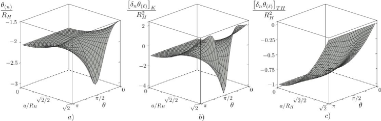
Figure 4: The FOTS defining quantities for a Kerr horizon. That $\theta_{(n)}<0$ everywhere on all Kerr horizons is shown by a) which graphs it for the standard scaling of the null vectors. However b) and c) demonstrate that the $\delta_{n}\theta_{(\ell)}<0$ condition is not so trivial. For the standard (131) scaling of the null vectors $\delta_{n}\theta_{(\ell)}$ can be positive and we must rescale as in equation (133) to show that the condition is always satisfied.

It is common to scale the null vectors so that $\ell^{a}$ is proportional to the global “time translation” Killing vector field on $H$ and the corresponding flow evolves the $v=\mbox{constant}$ two-surfaces into each other. Identifying this scaling with a sub/superscript-“$K$” we have

$$\ell_{K}^{a} = \left[1,0,0,\frac{a}{r^{2}+a^{2}}\right]\,\,\mbox{and}$$ (131)

$$n^{K}_{a} = \left[-1,\frac{a^{2}\sin^{2}\theta}{2(r^{2}+a^{2})},0,0\right]\,\,,$$

where the coordinate ordering is $\{v,r,\theta,\phi\}$. This is also the scaling for which the surface gravity is constant and takes the value

$$\kappa_{\ell}=\frac{1}{2r}\left(\frac{r^{2}-a^{2}}{r^{2}+a^{2}}\right)\,.$$ (132)

In Figures 4a and 4b we plot $\theta_{(n)}$ and $\delta_{n}\theta_{(\ell)}$ respectively for this scaling of the null vectors. It is immediately apparent that while $\theta_{(n)}<0$, horizons with sufficiently large angular momentum have $\delta_{n}\theta_{(\ell)}\geq 0$ over some region. However, this does not imply that for these horizons the $v=\mbox{constant}$ surfaces fail to be FOTHs. Instead it nicely demonstrates that different scalings of the null vectors generate different deformations of the two-surfaces and that not all of the resulting two-surfaces are fully trapped. If we rescale the null vectors to become

$$\ell_{TH}^{a}=\frac{1}{\Sigma}\ell_{K}^{a}\,\,\mbox{and}\,\,n^{TH}_{a}=\Sigma n^{K}_{a}\,,$$ (133)

then $\delta_{n}\theta_{(\ell)}$ calculated with respect to these vectors is everywhere negative, as shown in Figure 4c. Thus the $v=\mbox{constant}$ slices are FOTS, but the standard scaling of the Kerr null normals does not show this.

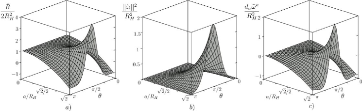
Figure 5: The quantities that determine $\delta_{n}\theta_{(\ell)}$ (which also appear in the first condition of the definition of a slowly expanding horizon) as calculated for the standard scaling of the null vectors (131).

Computationally we can understand what is happening for these two different scalings by considering the individual components that went into the calculations. Equation (37) tells us that in the absence of matter fields

$$\delta_{n}\theta_{(\ell)}=-\tilde{R}/2+|\mspace{-2.0mu}|\tilde{\omega}|\mspace{-2.0mu}|^{2}-d_{a}\tilde{\omega}^{a}\,.$$ (134)

Figure 5 graphs these quantities for the standard scaling (131) of the null vectors. The Ricci scalar is, of course, scaling invariant and Figure 5a shows that for horizons with large angular momentum it can be negative. Thus, the scaling dependent $d_{a}\tilde{\omega}^{a}$ term must be positive and large enough to compensate for this. However, a quick examination of the shapes of Figures 5b and 5c shows that for the standard rescaling, this term is also negative.

In fact these figures are also sufficient to show why the rescaling (133) resolves this problem — although in a slightly roundabout way. To see this we first note that for any (topologically) spherical surface embedded in a spacetime, there is always a scaling of the null vectors so that $d_{a}\tilde{\omega}^{a}=0$ (as discussed in JK ; isoGeom this ultimately follows from the Hodge decomposition theorem). For the two-surface under consideration this scaling is

$$\ell_{o}^{a}=\frac{1}{\sqrt{\Sigma}}\ell_{K}^{a}\,\,\mbox{and}\,\,n^{o}_{a}=\sqrt{\Sigma}n^{K}_{a}\,.$$ (135)

Taking this as a reference, equation (9) tells us that if $\ell^{a}=f\ell_{o}^{a}$ and $n_{a}=(1/f)n_{a}^{o}$ then

$$|\mspace{-2.0mu}|\tilde{\omega}|\mspace{-2.0mu}|^{2} = |\mspace{-2.0mu}|\tilde{\omega}_{o}|\mspace{-2.0mu}|^{2}+2\tilde{\omega}_{o}^{a}d_{a}\ln f+|\mspace{-2.0mu}|d\ln f|\mspace{-2.0mu}|^{2}\,\,\mathrm{and}$$ (136)

$$d_{a}\tilde{\omega}^{a} = d^{2}\ln f\,\,.$$ (137)

On an axisymmetric horizon, the second term on the right-hand side of (136) will vanish. Meanwhile, $|\mspace{-2.0mu}|\tilde{\omega}|\mspace{-2.0mu}|^{2}$ is invariant under a rescaling $f\rightarrow 1/f$, while $d_{a}\tilde{\omega}^{a}\rightarrow-d_{a}\tilde{\omega}^{a}$. Just such a rescaling is made in the change from the Killing normalized null vectors (131) to the FOTH normalized ones (133), where in this case $f=1/\sqrt{\Sigma}$. Thus, it follows that

$$\left[\delta_{n}\theta_{(\ell)}\right]_{TH}=-\tilde{R}/2+|\mspace{-2.0mu}|\tilde{\omega}_{K}|\mspace{-2.0mu}|^{2}+d_{a}\tilde{\omega}_{K}^{a}\,,$$ (138)

and in this case the $d_{a}\tilde{\omega}^{a}$ term is preciesly what is required to guarantee that $\delta_{n}\theta_{(\ell)}>0$ over the whole horizon.

Figure 5 also demonstrates that $\tilde{R}$, $|\mspace{-2.0mu}|\tilde{\omega}|\mspace{-2.0mu}|^{2}$, and $d_{a}\tilde{\omega}^{a}$ are each of order $1/R_{H}^{2}$ as required for a slowly expanding horizon. Combining this with the fact that the expansion parameter $C=0$ for the $v=\mbox{constant}$ two- surfaces, we confirm that the event horizon of a Kerr black hole is not only a FOTH but is also a slowly evolving horizon.

Finally, Figure 6 graphs the quantities that appear in (58) in the definition of a slowly expanding horizon. Although in this case their exact form doesn’t matter (since $C=\epsilon=0$), it is useful to note that they too are of order $1/R_{H}^{2}$. Thus, for perturbed Kerr solutions (58) will be satisfied and the horizon will be slowly expanding, as long as $C$ is sufficiently small.

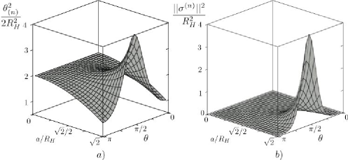
Figure 6: The quantities appearing in the definition of the slowly evolving parameter $\epsilon$ as calculated for the standard scaling of the null vectors (131).

References

- (1) S. W. Hawking and G. F. R. Ellis, The Large Scale Structure Sf spacetime (Cambridge University Press, 1973).
- (2) R. Penrose, Phys. Rev. Lett. 14 57 (1965).
- (3) D. M. Eardley Phys. Rev. D 57 2299 (1998).
- (4) R. M. Wald and V. Iyer, Phys. Rev. D 44 R3719 (1991).
- (5) E. Schnetter and B. Krishnan Phys. Rev. D 73 021502(R) (2006).
- (6) T. W. Baumgarte and S. L. Shapiro, Phys. Reports 376 41 (2003).
- (7) S. A. Hayward, Phys. Rev. D 49 6467 (1994).
- (8) S. A. Hayward, Phys. Rev. D 61 101503 (2000); Phys. Rev. D 64 044002 (2001); Class. Quant. Grav. 18 5561 (2001); Class. Quant. Grav. 23 L15 (2006).
- (9) S. A. Hayward, Phys. Rev. Lett. 93 251101 (2004); Phys. Rev. D 70 104027 (2004); “Conservation Laws for Dynamical Black Holes”, gr-qc/0607081.
- (10) A. Ashtekar, C. Beetle, O. Dreyer, S. Fairhurst, B. Krishnan, J. Lewandowski, J. Wisniewski, Phys. Rev. Lett. 85 3564 (2000).
- (11) A. Ashtekar, S. Fairhurst and B. Krishnan, Phys.Rev. D62 104025 (2000); A. Ashtekar, C. Beetle and J. Lewandowski, Phys.Rev. D64 044016 (2001).
- (12) J. Lewandowski and T. Pawlowski, Int. J. Mod. Phys. D 11 739 (2002); A. Ashtekar, C. Beetle, and J. Lewandowski, Class. Quant. Grav. 19 1195 (2002); J. Lewandowski and T. Pawlowski, Class. Quant. Grav. 20 587 (2003); J. Lewandowski and T. Pawlowski, “Symmetric non-expanding horizons”, gr-qc/ 0605026 (2006).
- (13) O. Dreyer, B. Krishnan, E. Schnetter and D. Shoemaker, Phys. Rev. D 67 024018 (2003).
- (14) T. Pawlowski, J. Lewandowski and J. Jezierski, Class. Quant. Grav. 21 1237 (2004).
- (15) A. Ashtekar and B. Krishnan, Phys.Rev.Lett. 89 261101 (2002); Phys. Rev. D68 104030 (2003).
- (16) A. Ashtekar and G. Galloway, Adv. Theor. Math. Phys. 9 1 (2005).
- (17) I. Booth and S. Fairhurst, Class. Quant. Grav. 22 4515 (2005).
- (18) L. Andersson, M. Mars, and W. Simon, Phys. Rev. Lett. 95 111102 (2005) .
- (19) E. Schnetter, B. Krishnan and F. Beyer Phys. Rev. D 74 024028 (2006).
- (20) I. Booth, L. Brits, J. A. Gonzalez and C. Van Den Broeck, Class. Quant. Grav. 23 413 (2006).
- (21) R. Bartnik and J. Isenberg, Class. Quant. Grav. 23 2559 (2006).
- (22) A. Nielsen and M. Visser, Class. Quant. Grav. 23 4637 (2006).
- (23) E. Gourgoulhon, Phys. Rev. D 72, 104007 (2005);
- (24) E. Gourgoulhon and J. L. Jaramillo, Phys. Rev. D 74, 087502 (2006).
- (25) M. Korzynski, “Isolated and dynamical horizons from a common perspective”, gr-qc/ 0605019.
- (26) I. Booth and S. Fairhurst, Phys. Rev. Lett. 92 011102 (2004).
- (27) W. Kavanagh and I. Booth, Phys. Rev. D 74 044027 (2006).
- (28) E. Gourgoulhon and J. L. Jaramillo , Phys. Rep. 423, 159 (2006).
- (29) A. Ashtekar and B. Krishnan, Liv. Rev. Relativity 7, 10 (2004).
- (30) I. Booth, Can. J. Phys. 83 1073 (2005).
- (31) L. Andersson and J. Metzger, “Curvature estimates for stable marginally trapped surfaces,” arXiv:gr-qc/0512106.
- (32) J. Brown and J.W. York, Phys. Rev. D 47 1407 (1993).
- (33) S. A. Hayward, Class. Quant. Grav. 10, 779 (1993).
- (34) R. Newman, Class. Quant. Grav. 4 277 (1987).
- (35) J. M. M. Senovilla, JHEP, 11 046 (2003).
- (36) I. Booth and S. Fairhurst, “Extremality conditions for dynamical horizons” (in preparation).
- (37) S. W. Hawking and J. B. Hartle, Commun. Math. Phys. 27 283 (1972).
- (38) I. Booth and S. Fairhurst, Class. Quant. Grav. 20 4507 (2003).
- (39) S. A. Hayward, Phys. Rev. D 74, 104013 (2006); Class. Quant. Grav. 24, 923 (2007).
- (40) M. Spivak, A comprehensive introduction to differential geometry : Volume 5, Third Edition (Publish or Perish, Inc. : Houston) (1999).
- (41) J. Jezierski, J. Kijowski and E. Czuchry, Rep. Math. Phys. 46 399-418 (2000).