Graviton mediated photon-photon scattering in general relativity

Abstract

In this paper we consider photon-photon scattering due to self-induced gravitational perturbations on a Minkowski background. We focus on four-wave interaction between plane waves with weakly space and time dependent amplitudes, since interaction involving a fewer number of waves is excluded by energy-momentum conservation. The Einstein-Maxwell system is solved perturbatively to third order in the field amplitudes and the coupling coefficients are found for arbitrary polarizations in the center of mass system. Comparisons with calculations based on quantum field theoretical methods are made, and the small discrepances are explained.

I Introduction

As is wellknown, photon-photon scattering can occur due to the exchange of virtual electron-positron pairs, as described by QED or modifications thereof, see e.g. QED-general , and may even lead to collective photon phenomena collective . Photon interactions via the quantum vacuum, sometimes involving deviations from the standard model, has recently been much discussed in the literature due to advances in experimental technologies (see e.g. exp ) as well as new theoretical insights new . Moreover, photons also interact gravitationally, although this effect has been much less studied. Purely general relativistic treatments of electromagnetic wave interactions have been made resulting in exact solutions, see e.g. Griffiths91 , but these calculations are very different from the pure scattering processes, and do not address the interaction at the single photon level. On the other hand, it is not clear to what extent calculations of the gravitational cross-section using quantum field theoretical methods Barker1966 ; Barker1967 (see also Dewitt ) are consistent with classical general relativity. In order to shed light on this issue, we will consider the interaction of four electromagnetic (EM) waves on a Minkowski background, which is the lowest order scattering process consistent with energy-momentum conservation. By studying the classical Einstein-Maxwell system, but ignoring terms that do not correspond to pure scattering (e.g. frequency shift terms) we will attempt to make contact between the classical and quantum field theoretical picture. Calculating the classical coupling coefficients between waves of different polarizations, corresponding to the scattering amplitudes in quantum field theory, we are able to compare the classical cross-section with that of quantum field theory Barker1966 ; Barker1967 . While the results are approximately equal for small scattering angles $\theta$, we find that there are significant differences for large $\theta$. The likely source behind this discrepancy is that the quantum field theoretical calculation Barker1967 used the matrix scattering amplitude in order to define the interaction potential. As shown by Ref. Kazakov2001 , such a procedure is not able to fully reproduce the general relativistic potential.

Finally we note that while gravitational photon-photon scattering is weaker than the QED scattering in most cases of physical interest QED-general ; collective , it should be noted that in the long wavelength limit, actually the gravitational cross-section is larger than that due to QED.

II Theory and results

We employ units such that the speed of light and Planck’s constant are $c=\hbar=1$, and use metric signature $\left(-,+,+,+\right)$. Tetrad indices $a,b,\ldots$ run from 0 to 3 and $\alpha,\beta,\ldots$ from 1 to 3. Coordinate indices $\mu,\nu,\ldots$ go from 0 to 3.
Assuming plane waves and denoting the interacting waves $A$, $B$, $C$ and $D$ the total electric field is given by

$$E=\sum_{n}\left[E_{n}(x^{\mu})e^{ik_{n\mu}x^{\mu}}+\mathrm{c.c.}\right]\hskip 5.69054pt,\hskip 5.69054ptn=A,B,C,D,$$

where c.c. denotes the complex conjugate. A similar expression holds for the magnetic field. Moreover we assume that the amplitudes have a weak dependence on space and time, i.e. $\left|\partial_{\mu}E\left(x^{\nu}\right)\right|\ll\left|k_{\mu}\right|\left|E\left(x^{\nu}\right)\right|$. The presence of the EM fields induce a perturbation, $h_{\mu\nu}$, of the flat background metric, $\eta_{\mu\nu}$, enabling energy exchange between the modes. A generic frame, orthonormal to quadratic order in the field amplitudes (linear order in the metric perturbation), is chosen as

$$e_{0}^{\mu} = \left(1+\frac{1}{2}h_{00},-\frac{1}{2}h_{01},-\frac{1}{2}h_{02},-\frac{1}{2}h_{03}\right),$$

$$e_{1}^{\mu} = \left(\frac{1}{2}h_{01},1-\frac{1}{2}h_{11},-\frac{1}{2}h_{12},-\frac{1}{2}h_{13}\right),$$

$$e_{2}^{\mu} = \left(\frac{1}{2}h_{02},-\frac{1}{2}h_{12},1-\frac{1}{2}h_{22},-\frac{1}{2}h_{23}\right),$$

$$e_{3}^{\mu} = \left(\frac{1}{2}h_{03},-\frac{1}{2}h_{13},-\frac{1}{2}h_{23},1-\frac{1}{2}h_{33}\right)\hskip 5.69054pt,$$ (1)

where $\mathbf{e}_{a}=e_{a}^{\mu}\partial_{\mu}$. The matching condition corresponding to energy and momentum conservation is given by

$$k_{A}^{\mu}+k_{B}^{\mu}=k_{C}^{\mu}+k_{D}^{\mu}\hskip 5.69054pt.$$ (2)

In the center of mass system all frequencies are equal and the waves are counterpropagating pairwise, i.e. the wave vectors satisfy $\mathbf{k}_{A}=-\mathbf{k}_{B}$, $\mathbf{k}_{C}=-\mathbf{k}_{D}$. We make the following ansatz for the metric perturbations

$$\!\!\!\!\!\!\!h_{\alpha\beta}=\bar{h}_{\alpha\beta}\left(x,z,t\right)e^{-2i\omega t}+\bar{h}_{\alpha\beta}^{\ast}\left(x,z,t\right)e^{2i\omega t}$$

$$\!\!\!\!\!\!+\tilde{h}_{\alpha\beta}\left(t,x,z\right)e^{-i\left(\mathbf{k}_{A}+\mathbf{k}_{C}\right)\cdot\mathbf{x}}+\tilde{h}_{\alpha\beta}^{\ast}\left(t,x,z\right)e^{i\left(\mathbf{k}_{A}+\mathbf{k}_{C}\right)\cdot\mathbf{x}}$$

$$\!\!\!\!\!\!+\hat{h}_{\alpha\beta}\left(t,x,z\right)e^{-i\left(\mathbf{k}_{A}-\mathbf{k}_{C}\right)\cdot\mathbf{x}}+\hat{h}_{\alpha\beta}^{\ast}\left(t,x,z\right)e^{i\left(\mathbf{k}_{A}-\mathbf{k}_{C}\right)\cdot\mathbf{x}}.$$

This is not the most general ansatz, however it is sufficient to give all terms corresponding to resonant energy exchange between the modes. All the components $\bar{h}_{\alpha\beta}$, $\bar{h}_{\alpha\beta}^{\ast}$, $\tilde{h}_{\alpha\beta}$, $\tilde{h}_{\alpha\beta}^{\ast}$, $\hat{h}_{\alpha\beta}$, $\hat{h}_{\alpha\beta}^{\ast}$, except twelve of them, are determined by the field equations, $G_{ab}=\kappa T_{ab}$, where $G_{ab}$ is the Einstein tensor and $T_{ab}$ the energy-momentum tensor. In the present case the only contribution to the energy-momentum tensor is given by

$$T_{ab}=F_{a}^{c}F_{bc}-\tfrac{1}{4}g_{ab}F^{cd}F_{cd}\hskip 5.69054pt.$$

The undetermined coefficients in the metric ansatz are set to zero using the generalized Lorentz condition. Note that the non-zero coefficients are of quadratic order in the field amplitudes. Using Maxwell’s equations $\nabla_{[a}F_{bc]}=0$ and $\nabla_{a}F^{ab}=j^{b}$, where $F^{ab}$ is the electromagnetic field tensor and $j^{b}$ the four-current density, we can derive the following wave equations

$$\tilde{\square}E^{\alpha} = -\mathbf{e}_{0}j_{E}^{\alpha}-\epsilon^{\alpha\beta\gamma}\mathbf{e}_{\beta}j_{B\gamma}-\delta^{\alpha\gamma}\mathbf{e}_{\gamma}\rho_{E}-$$ (3)

$$\epsilon^{\alpha\beta\gamma}C_{\beta 0}^{a}\mathbf{e}_{a}B_{\gamma}-\delta^{\alpha\gamma}C_{\beta\gamma}^{a}\mathbf{e}_{a}E^{\beta}\hskip 17.07164pt,$$

$$\tilde{\square}B^{\alpha} = -\mathbf{e}_{0}j_{B}^{\alpha}+\epsilon^{\alpha\beta\gamma}\mathbf{e}_{\beta}j_{E\gamma}-\delta^{\alpha\gamma}\mathbf{e}_{\gamma}\rho_{B}+$$ (4)

$$\epsilon^{\alpha\beta\gamma}C_{\beta 0}^{a}\mathbf{e}_{a}E_{\gamma}-\delta^{\alpha\gamma}C_{\beta\gamma}^{a}\mathbf{e}_{a}B^{\beta}.\hskip 14.22636pt$$

Here the wave operator $\tilde{\square}\equiv\mathbf{e}_{0}\cdot\mathbf{e}_{0}+\nabla\cdot\nabla$, which coincides with the D’Alembertian operator in Euclidian space, and $C_{ab}^{c}$ are commutation functions for the frame vectors satisfying $\left[\mathbf{e}_{a},\mathbf{e}_{b}\right]=C_{ab}^{c}\mathbf{e}_{c}$. $\mathbf{j}_{E}$, $\mathbf{j}_{B}$, $\rho_{E}$ and $\rho_{B}$ are the effective currents and charges due to the inclusion of the gravitational field given by

$$\mathbf{j}_{E} = \Big{[}-\left(\Gamma_{0\beta}^{\alpha}-\Gamma_{\beta 0}^{\alpha}\right)E^{\beta}+\Gamma_{0\beta}^{\beta}E^{\alpha}-$$ (5)

$$\epsilon^{\alpha\beta\gamma}\left(\Gamma_{\beta 0}^{0}B_{\gamma}+\Gamma_{\beta\gamma}^{\delta}B_{\delta}\right)\Big{]}\mathbf{e}_{\alpha}\hskip 5.69054pt,$$

$$\mathbf{j}_{B} = \Big{[}-\left(\Gamma_{0\beta}^{\alpha}-\Gamma_{\beta 0}^{\alpha}\right)B^{\beta}+\Gamma_{0\beta}^{\beta}B^{\alpha}-$$ (6)

$$\epsilon^{\alpha\beta\gamma}\left(\Gamma_{\beta 0}^{0}E_{\gamma}+\Gamma_{\beta\gamma}^{\delta}E_{\delta}\right)\Big{]}\mathbf{e}_{\alpha}\hskip 5.69054pt,$$

$$\rho_{E} = -\Gamma_{\beta\alpha}^{\alpha}E^{\beta}-\epsilon^{\alpha\beta\gamma}\Gamma_{\alpha\beta}^{0}B_{\gamma}\hskip 5.69054pt,$$ (7)

$$\rho_{B} = -\Gamma_{\beta\alpha}^{\alpha}B^{\beta}-\epsilon^{\alpha\beta\gamma}\Gamma_{\alpha\beta}^{0}E_{\gamma}\hskip 5.69054pt,$$ (8)

where $\Gamma_{bc}^{a}$ are the Ricci rotation coefficients. The effective currents and charges will be of cubic order in the field amplitudes. Eliminating the magnetic field from the wave equation (3) by using Faraday’s law to leading order, $\mathbf{k}\times\mathbf{E}=\omega\mathbf{B}$, and neglecting terms of order four or higher in the field amplitudes will result in three categories of terms.

1. Nonresonant terms that will vanish after averaging over several wavelengths and time periods. Interaction due to these terms are not consistent with energy momentum conservation. Most terms belong in this category.

2. Phase shift terms which are resonant but give rise to phase shifts rather than scattering. These terms typically contain a certain amplitude together with its complex conjugate, i.e. terms of the form $E_{A}E_{A}^{\ast}E_{B}$.

3. Resonant scattering terms containing all three wave amplitudes according to the energy-momentum conservation condition (2).

Based on the classification of terms above we restrict ourselves to include only the resonant scattering terms and introduce polarization states perpendicular to the wave vectors as shown in figure 1. Note that the $E_{2}$ and the $E_{\times}$ directions coincide. We thus have

$$E_{A1}=-\cos\left({\theta}/{2}\right)E_{A+},\quad E_{A3}=\sin\left({\theta}/{2}\right)E_{A+},$$

$$E_{B1}=\cos\left({\theta}/{2}\right)E_{B+},\quad\,\,\,\,\,E_{B3}=-\sin\left({\theta}/{2}\right)E_{B+},$$

$$E_{C1}=-\cos\left({\theta}/{2}\right)E_{C+},\quad E_{C3}=-\sin\left({\theta}/{2}\right)E_{C+},$$

$$E_{D1}=\cos\left({\theta}/{2}\right)E_{D+},\quad\,\,\,\,\,E_{D3}=\sin\left({\theta}/{2}\right)E_{D+},$$

with $E_{A2}=E_{A\times},E_{B2}=E_{B\times},E_{C2}=E_{C\times},E_{D2}=E_{D\times}$, and

$$k_{Ax} = \sin\left({\theta}/{2}\right)\omega,\hskip 14.22636ptk_{Az}=\cos\left({\theta}/{2}\right)\omega,$$

$$k_{Bx} = -\sin\left({\theta}/{2}\right)\omega,\hskip 5.69054ptk_{Bz}=-\cos\left({\theta}/{2}\right)\omega,$$

$$k_{Cx} = -\sin\left({\theta}/{2}\right)\omega,\hskip 5.69054ptk_{Cz}=\cos\left({\theta}/{2}\right)\omega,$$

$$k_{Dx} = \sin\left({\theta}/{2}\right)\omega,\hskip 14.22636ptk_{Dz}=-\cos\left({\theta}/{2}\right)\omega.$$

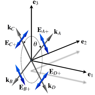
Figure 1: Polarization directions and the definition of the scattering angle $\theta$.

After some lengthy but straightforward algebra we end up with the following coupling equations describing the evolution of the wave amplitudes to leading order

$$\square E_{A+} = F_{1}E_{B+}^{\ast}E_{C+}E_{D+}+F_{2}E_{B+}^{\ast}E_{C\times}E_{D\times}$$ (9)

$$+F_{3}E_{B\times}^{\ast}E_{C\times}E_{D+}+F_{4}E_{B\times}^{\ast}E_{C+}E_{D\times},$$

$$\square E_{B+} = F_{1}E_{A+}^{\ast}E_{C+}E_{D+}+F_{2}E_{A+}^{\ast}E_{C\times}E_{D\times}$$ (10)

$$+F_{3}E_{A\times}^{\ast}E_{C+}E_{D\times}+F_{4}E_{A\times}^{\ast}E_{C\times}E_{D+},$$

$$\square E_{C+} = F_{1}E_{D+}^{\ast}E_{A+}E_{B+}+F_{2}E_{D+}^{\ast}E_{A\times}E_{B\times}$$ (11)

$$+F_{3}E_{D\times}^{\ast}E_{A\times}E_{B+}+F_{4}E_{D\times}^{\ast}E_{A+}E_{B\times},$$

$$\square E_{D+} = F_{1}E_{C+}^{\ast}E_{A+}E_{B+}+F_{2}E_{C+}^{\ast}E_{A\times}E_{B\times}$$ (12)

$$+F_{3}E_{C\times}^{\ast}E_{A+}E_{B\times}+F_{4}E_{C\times}^{\ast}E_{A\times}E_{B+},$$

where $\square=\partial^{2}/\partial t^{2}-\partial^{2}/\partial x^{2}-\partial^{2}/\partial z^{2}$ and

$$F_{1}=\frac{\kappa\left(3+\cos^{2}\theta\right)^{2}}{1-\cos^{2}\theta},\hskip 5.69054pt$$

$$F_{2}=-\kappa\left(7+\cos^{2}\theta\right),$$

$$F_{3}=\frac{4\kappa\left(2+\cos^{2}\theta+\cos\theta\right)}{1+\cos\theta},\hskip 5.69054pt$$

$$F_{4}=\frac{4\kappa\left(2+\cos^{2}\theta-\cos\theta\right)}{1-\cos\theta}.$$ (13)

For symmetry reasons $\square E_{A\times},\square E_{B\times},\square E_{C\times}$ and $\square E_{D\times}$ can be found from (9)–(12) respectively by interchanging $+$ and $\times$. The coupling coefficients only depend on the scattering angle $\theta$, and in the limit when $\theta\rightarrow 0$ both $F_{1}$ and $F_{4}$ become infinite while $F_{2}\rightarrow-F_{3}$. The small angle divergence in $F_{1}$ and $F_{4}$ is a consquence of the infinite range of the gravitational force. However, the coefficients $F_{2}$ and $F_{3}$ must remain finite for all angles, as those coefficients not only describe scattering an angle $\theta$, but also correspond to a change in the polarization state.

In order to check the consistency of our results, we assume long pulses, i.e. $\square\approx-2i\omega\partial_{t}$, such that the time derivative of the total energy density, $\varepsilon_{tot}=\sum_{n}(|E_{n+}|^{2}+|E_{n\times}|^{2})$ (where the sum is over $A,B,C,D$), can be easily calculated. Carrying out the sum, it is found that all the scattering terms cancel, and thus we deduce that the evolution equations (9)-(12) are energy conserving.

Next we rewrite (9)–(12) in terms of the vector potentials, which rescales the coupling coefficients (13) by a factor $\omega^{2}$. Noting that the rescaled coupling coefficients corresponds to the scattering amplitudes, and following Ref. Itzykson85 , we find that the unpolarized differential cross-section can be calculated as

$$\frac{\partial\sigma}{\partial\Omega}=\frac{\left|\mathcal{M}\right|^{2}}{128\omega^{2}\left(2\pi\right)^{2}}\hskip 5.69054pt,$$ (14)

where the square of the scattering matrix amplitude averaged over all polarization states is given by

$$\left|\mathcal{M}\right|^{2} = \frac{\omega^{4}\kappa^{2}}{\sin^{4}\theta}\left(\cos^{8}\theta+28\cos^{6}\theta+70\cos^{4}\theta\right.$$ (15)

$$\qquad\qquad\left.+28\cos^{2}\theta+129\right).$$

This result should be compared with the same quantity calculated by quantum field theoretical methods, i.e. Eq. (15) in Ref. Barker1967 . It turns out that the differential cross-sections agree in the limit $\theta\ll\pi/2$, but as seen from Fig 2, where the classical and quantum field theoretical expressions are shown, the two expressions differ slightly in general. In order to resolve the difference more accurately, the ratio of the cross-sections are shown in Fig. 3, where one should note the agreement for small angles. However, for general angles the expressions clearly disagree, and it is natural to ask what causes this discrepancy. To answer this question we note that Ref. Barker1967 has used the matrix scattering amplitude to determine the interaction potential. As demonstrated by Ref. Kazakov2001 , however, such a procedure is not sufficient to fully reproduce the general relativistic potential. As the general relativistic deviation from Newtonian behavior becomes more pronounced for large scattering angles, this explains the deviation for general angles, but also the agreement in the small angle limit.

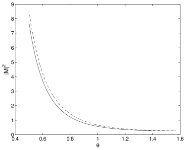
Figure 2: The classical(solid line)and quantum field theoretical (dashed line) cross-sections in arbitrary units as a function of scattering angle.

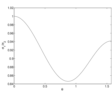
Figure 3: The ratio of the classical and quantum field theoretical cross-sections $\sigma_{1}$ and $\sigma_{2}$, respectively, as a function of scattering angle.

III Summary and Discussion

Comparing the calculated cross-section for gravitational photon-photon scattering Eq. (14) with that from QED photon-photon scattering (due to exchange of virtual electron-positron pairs), we find that they have different frequency dependence. The former is proportional to $\omega^{2}$ while the latter is proportional to $\omega^{6}$ Itzykson85 . Noting from Eq. (14) that $\partial\sigma/\partial\Omega\approx 16(2\pi)^{2}L_{p}^{4}/\lambda^{2}$ (letting $\sin\theta\sim\cos\theta\sim 1/\sqrt{2}$), where $L_{p}$ is the Planck length and $\lambda$ the wavelength, and comparing with the QED expression for the cross-section (e.g. Ref. Itzykson85 ), we find that the QED and gravitational cross-sections are comparable for frequencies

$$\omega\sim 10^{3}c\left({L_{p}^{2}}/{r_{0}\lambda_{c}^{3}}\right)^{1/2},$$ (16)

where $r_{0}$ is the classical electron radius, $\lambda_{c}$ is the Compton wavelength, and we have reinstated the speed of light $c$. Thus the gravitational effects become the dominant contribution to the cross-section for frequencies $\omega\sim 30\,\rm{rad/s}$ and lower. Still, the cross-section is very small, and we need extremely large photon densities for gravitational photon-photon scattering to influence the dynamics. Situations that could be of interest to study in more detail involve the dense photon gas surrounding pulsars Kondratyev , as well as the photon gas in the early universe Kolb-Turner . Furthermore, we note that if the energy densities are sufficiently high Sufficient-note , the timescales for nonlinear evolution will not be determined by the cross-section, even if the spectrum is strongly incoherent. Instead the characteristic time-scale must be found from weak turbulence theories Hasegawa-book . Using the so called random phase approximation, the phase dependence can be integrated out, and evolution equations for the spectral energy densities are derived Hasegawa-book .

Graviton mediated photon-photon scattering share many parameter similarities with photon-graviton pair conversion Andreas . While it is possible that gravitational photon-photon scattering may have applications to astrophysics and/or cosmology, the effect can typically be neglected compared to other effects, such as QED photon-photon scattering or, in the presence of matter, interaction with charged particles. Thus our main aim here has been to make an explicit comparison with the quantum field theoretical result (see Fig. 2), which show a slight deviation from our general relativistic cross-section. As seen in Fig. 3, the deviation vanishes in the limit of small scattering angles. We trace the difference between the quantum field theoretical and the classical result to the difficulty in determining the general relativistic interaction potential from the matrix scattering amplitude, as done by Ref. Barker1967 . An interesting problem, which is a project for further research, is to investigate whether a quantum field theoretical calculation can be improved to incorporate a fully general relativistic interaction potential.

References

• (1) W. Heisenberg H. and Euler H., Z. Physik 98, 714 (1936); J. Schwinger J., Phys. Rev. 82, 664 (1951). G. Brodin, M. Marklund and L. Stenflo, Phys. Rev. Lett. 87, 171801 (2001).
• (2) M. Marklund, G. Brodin, and L. Stenflo, Phys. Rev. Lett. 91, 163601 (2003); M. Marklund, G. Brodin, L. Stenflo, and P. K. Shukla, Phys.Scripta T107, 239 (2004); M. Marklund and P. K. Shukla, Rev. Mod. Phys. 78, 591 (2006).
• (3) G. A. Mourou, T. Tajima, and S. V. Bulanov, Rev. Mod. Phys. 78, 309 (2006); Y. I. Salamin, S. X. Hu, K. Z. Hatsagortsyan, and C. H. Keitel, Phys. Rep. 427, 41 (2006).
• (4) E. Lundström et al., Phys. Rev. Lett. 96, 083602 (2006); E. Zavattini et al., Phys. Rev. Lett. 96, 110406 (2006); R. Rabadan, A. Ringwald, and K. Sigurdson, Phys. Rev. Lett. 96, 110407 (2006); B. A. van Tiggelen, G. L. J. A. Rikken, and V. Krstic, Phys. Rev. Lett. 96, 130402 (2006); D. B. Blaschke, A. V. Prozorkevich, C. D. Roberts, S. M. Schmidt, and S. A. Smolyansky, Phys. Rev. Lett. 96, 140402 (2006); A. Di Piazza, K. Z. Hatsagortsyan, and C. H. Keitel, Phys. Rev. Lett. 97, 083603 (2006); J. T. Mendonça, J. Dias de Deus, and P. C. Ferreira, Phys. Rev. Lett. 97, 100403 (2006); R. Schützhold, G. Schaller and D. Habs, Phys. Rev. Lett. 97, 121302 (2006).
• (5) J. B Griffiths, Colliding Plane Waves in General Relativity, Clarendon Press, Oxford (1991)
• (6) B. M. Barker, S. N. Gupta and R. D. Haracz, Phys. Rev., 149, 1027 (1966).
• (7) B. M. Barker, M. S. Bathia and S. N. Gupta, Phys. Rev., 158, 1498 (1967).
• (8) B. S. Dewitt, Phys. Rev. 160, 1113 (1967); ibid. 162, 1195 (1967); ibid. 162, 1239 (1967).
• (9) K. A. Kazakov, Class. Quant. Grav. 18, 1039 (2001).
• (10) C. Itzykson and J. B. Zuber, Quantum Field Theory, (McGraw-Hill Book Co., Singapore, 1985)
• (11) V. N. Kondratyev, Phys. Rev. Lett. 88, 221101 (2002).
• (12) E. Kolb and M. Turner, The Early Universe (Addison-Wesley, 1988)
• (13) A ”sufficiently high” photon density here means that the number of photons present in a cube of size $\lambda_{\mathrm{ch}}^{3}$, where $\lambda_{\mathrm{ch}}$ is the characteristic wavelength of the spectrum, is much larger than unity. Note that for a photon gas subject to cosmological  expansion, this number is a constant. Furthermore, for the particular case of the cosmic background radiation, this constant is much smaller than unity.
• (14) A. Hasegawa, Plasma Instabilities and Nonlinear Effects, Chap. 4.3. (Springer-Verlag, Berlin, 1975).
• (15) A. Källberg, G. Brodin, and M. Marklund, Class. Quantum Grav. 23, L7 (2006).