Brane Cosmology in an Arbitrary Number of Dimensions

N. Chatillon, C. Macesanu and M. Trodden

Department of Physics, Syracuse University, Syracuse, NY 13244-1130, USA.

Abstract

We derive the effective cosmological equations for a non-$\mathbb{Z}_{2}$ symmetric codimension one brane embedded in an arbitrary D-dimensional bulk spacetime, generalizing the $D=5,6$ cases much studied previously. As a particular case, this may be considered as a regularized codimension (D-4) brane avoiding the problem of curvature divergence on the brane. We apply our results to the case of spherical symmetry around the brane and to partly compactified AdS-Schwarzschild bulks.

1 Introduction

The possibility of extra spatial dimensions, in addition to the three that we perceive in everyday life, is a crucial aspect of a number of constructions in modern particle physics, from string theory to methods to address the hierarchy problem [1, 2, 3, 4, 5, 6, 7, 8, 9, 10, 11, 12, 13, 14]. In many of these models, the matter content of our three-dimensional universe is confined to a submanifold, or 3-brane, while gravity, via the equivalence principle, propagates in the entire space-time, or bulk.

Large extra dimension models with matter localized on a 4d brane have been re-popularized recently by their application to the electroweak hierarchy problem [6, 7]. In these models the bulk metric, typically a flat hypertorus, is assumed to be unaffected by the energy-momentum content of the brane, which allows for a formulation independently of the total dimension. At the background level, this is justified by the absence of a brane tension. The effect of the brane matter is less trivial in general. For energies small compared to the typical inverse radius $R^{-1}$ of the bulk, the Kaluza-Klein (KK) zero-mode truncation applies as a valid approximation for the bulk metric. The non-trivial curvature induced on the bulk metric may be studied above these energies by including the tower of non-zero KK gravitons as effective 4d particles. Brane-world cosmology with flat bulk has received much careful study, although previous work has mostly focused on the low-energy regime (although far above $R^{-1}$), under a “normalcy temperature” $T_{*}$ evaluated in [15, 16], where the bulk size is assumed to have been already stabilized by an unspecified high-energy mechanism and the non-zero KK gravitons do not have a significant effect on the evolution of the brane metric. The effect of brane matter on the bulk metric evolution at earlier times, and the consequent alteration of the brane metric evolution, has not yet been studied systematically in an arbitrary number of dimensions.

The problem extends to unwarped brane models with non-flat but homogeneous transverse space. The conclusions of cosmological studies where the brane is a point in a compact hyperbolic transverse space [17, 18], for instance, are valid only as long as the brane content does not significantly alter the bulk homogeneity condition.

Another very interesting class of brane models considers the cosmological evolution resulting from an induced kinetic term for gravity localized on the brane in addition to the bulk one [19, 20, 21, 22, 23, 24, 25, 26] ; we focus here on the more simple case of models with pure bulk gravity.

Compact and non-compact models with extra dimensions warped by the presence of a large brane tension provide an elementary example in which the backreaction effect is taken into account. In five dimensions, the brane is codimension one and leads to an exponential warping useful for explaining the Standard Model hierarchies as a gravitational effect [8], or for localizing gravity with non-compact bulks [9]. However, here again it is a non-trivial task to treat the backreaction of a more general cosmological brane source beyond the zero-mode approximation.

In five and six dimensions, exact and perturbative results have been obtained for such a source. In the simplest case, the cosmological evolution of a brane with tension $\lambda$ in an infinite $D=5$ bulk leads to exactly calculable $O(\rho^{2}/\lambda^{2})$ corrections to the Friedmann equation [27]. The compact case is more subtle as one must also allow for the evolution of the radion field [28]. The aberrant Hubble rate, quadratic in $\rho$ for $D=5$ flat compact bulks [29, 30] for instance, has been shown [31] to result from the unnatural requirement of a static radion without introducing a stabilization mechanism, which leads to an overconstraint on the extra matter on a second brane. Stabilized models treated perturbatively in $\rho$ again lead to a correct Friedmann equation, linear in $\rho$ with quadratic corrections [32]. We leave the review and discussion of more general five-dimensional configurations, including non-$\mathbb{Z}_{2}$ symmetric bulks and “dark radiation” terms, for section 3.

The problem is qualitatively different for a codimension two brane in $D=6$, a configuration reminiscent of the much studied cosmic string solutions in four dimensions. Indeed, for any brane source differing from a pure tension, the curvature diverges on the brane on which observers are supposed to live. This problem has been solved by considering regularized or “fat” branes with finite width. In the simple case of the compact “football” shaped bulk solution whose size is stabilized by a bulk magnetic flux [33, 34], the Friedmann equation once again exhibits perturbative $\rho^{2}$ corrections at high energies [35, 36]. Backreaction effects in cosmological brane models for $D>6$ remain to be investigated.

Since it is expected that higher codimension infinitely thin branes will be singular, regularization is necessary, by an homogeneous spherical core for example. Alternatively, if the brane matter is taken to be localized at the boundary of this core (see figure 3), the codimension (D-4) brane is regularized as an infinitely thin codimension one brane shell with a (D-1)-dimensional worldvolume. The extra (D-5) spatial dimensions on the worldvolume in addition to the three observable ones may then be eliminated by compactification with a sufficiently small radius.

In this paper, we derive the effective cosmological equations for a non-$\mathbb{Z}_{2}$ symmetric codimension one brane embedded in an arbitrary D-dimensional bulk spacetime. Our results generalize the $D=5,6$ cases which have been exhaustively studied previously by other authors, exactly in the case of infinitely thin branes for $D=5$, and perturbatively with regularized core branes for $D=6$. As we shall see, in the case of higher codimension, there is significantly more choice for the bulk geometry and hence, in the equivalent 4-dimensional effective theory, for the nature of the extra terms induced in the Friedmann equation.

The paper is organized as follows. In the next section we review the derivation of the Einstein equations induced on the brane in an arbitrary number of dimensions. In section 3 we consider the case of a general unspecified bulk with spherical symmetry around the brane, including non-$\mathbb{Z}_{2}$ symmetric contributions. We then derive a non-conservation law for the dark radiation specific to $D>5$ brane models, and we apply our findings to a specific non-compact orbifold bulk. In section 4 we take the example of an AdS-Schwarzschild bulk in which spherical symmetry is broken by a toroidal compactification of the transverse space on the brane. In section 5 we provide a discussion of our results and conclude.

2 Brane gravity in an arbitrary number of dimensions

2.1 The Effective Einstein equations

The brane is taken to be a $(D-1)$-dimensional hypersurface, a particular member of a foliation of an unspecified $D-$dimensional spacetime, referred to as the bulk in what follows. Defining as $n^{a}$ the unit spacelike vector normal to the brane, the induced metric on the brane is then $\tilde{g}_{ab}=g_{ab}-n_{a}n_{b}$. The Gauss-Codazzi equations, with no dynamical assumptions, geometrically relate the bulk Riemann tensor ${\cal R}^{a}_{\ bcd}$ to the brane one $\tilde{\cal R}^{m}_{\ npq}$ (built from its induced metric $\tilde{g}_{ab}$) and to the extrinsic curvature tensor on the brane, given by

$$K_{ab}=K_{ba}=-\tilde{g}^{c}_{\ a}\ \tilde{g}^{d}_{\ b}\ \nabla_{c}n_{d}\ .$$ (2.1)

They read respectively

$${\cal R}^{a}_{\ bcd}\ \tilde{g}_{a}^{\ m}\ \tilde{g}^{b}_{\ n}\ \tilde{g}^{c}_{\ p}\ \tilde{g}^{d}_{\ q} = \tilde{\cal R}^{m}_{\ npq}+K^{m}_{\ q}K_{np}-K^{m}_{\ p}K_{nq}$$ (2.2)

$${\cal R}_{ab}\ \tilde{g}^{a}_{\ c}\ n^{b} = \tilde{\nabla}_{e}K^{e}_{\ c}-\tilde{\nabla}_{c}K\ ,$$ (2.3)

where $\tilde{\nabla}$ is the covariant derivative adapted to the brane induced metric.

Including gravitational dynamics, the Gauss equation (2.2) can be used to covariantly obtain the projected Einstein equations for the induced metric, to which brane observers are assumed to be minimally coupled. To achieve this, one first decomposes the bulk Riemann tensor into its algebraically irreducible components:

$${\cal R}^{ab}_{\ \ cd}=C^{ab}_{\ \ cd}+\frac{1}{D-2}\delta^{[a}_{\ [c}\Big{(}{\cal R}^{b]}_{\ d]}-\frac{1}{D}\delta^{b]}_{\ d]}{\cal R}\Big{)}+\frac{1}{2D(D-1)}\delta^{[a}_{\ [c}\delta^{b]}_{\ d]}{\cal R}\ ,$$ (2.4)

where $M_{[ab]}\equiv M_{ab}-M_{ba}$, and $C^{ab}_{\ \ cd}$ is the Weyl tensor, possessing the same symmetries as the Riemann tensor, plus total tracelessness. The Ricci tensor ${\cal R}^{a}_{\ b}$ is algebraically related to the bulk energy-momentum tensor ${\bf T}^{a}_{\ b}$ through the bulk Einstein equations

$${\cal R}^{a}_{\ b}=8\pi G_{D}\Big{(}{\bf T}^{a}_{\ b}-\frac{1}{D-2}{\bf T}\delta^{a}_{\ b}\Big{)}\ ,$$ (2.5)

where $G_{D}$ is the bulk (fundamental) Newton’s constant. The Weyl tensor describes gravitational radiation in the bulk, and is solved for using the bulk Bianchi identities $\nabla_{[a}{\cal R}_{bc]de}=0$ after expressing the Riemann tensor as a function of $C_{abcd}$ and ${\bf T}_{ab}$.

After contraction, (2.2) may be expressed as

$$\tilde{G}^{m}_{\ n} = 8\pi G_{D}\frac{D-3}{D-2}\ \Big{[}\ {\bf T}^{a}_{\ b}\ \tilde{g}^{m}_{\ a}\ \tilde{g}^{b}_{\ n}-\frac{1}{D-1}\ \tilde{g}^{m}_{\ n}\ {\bf T}^{a}_{\ b}\ \tilde{g}^{b}_{\ a}\Big{]}+8\pi G_{D}\frac{D-3}{D-1}\Big{(}{\bf T}^{a}_{\ b}\ n_{a}\ n^{b}\ \Big{)}\tilde{g}^{m}_{\ n}$$ (2.6)

$$-E^{m}_{\ n}+KK^{m}_{\ n}-K^{mp}K_{pn}-\frac{1}{2}\tilde{g}^{m}_{\ n}(K^{2}-K_{pq}K^{pq})\ ,$$

where $\tilde{G}_{mn}$ is the Einstein tensor constructed from the induced metric. In addition to the part linear in the bulk energy-momentum tensor ${\bf T}_{mn}$, these effective Einstein equations can be seen to contain source terms quadratic in the brane extrinsic curvature tensor, plus a tensor contribution, $E_{mn}$, defined from the bulk Weyl tensor by

$$E_{mn}\equiv C^{a}_{\ mcn}n_{a}n^{c}\ .$$ (2.7)

This last term is well known to embody the non-local effects of the bulk geometry (as opposed to ${\bf T}_{mn}$) on the brane matter dynamics. Being symmetric and traceless, it can be interpreted here as ($-8\pi G_{D}$ times) the energy-momentum tensor of a conformally invariant source, that we will call from now on dark radiation, borrowing the familiar terminology from the $D=5$ case applied to cosmological perfect fluids. Loosely speaking, this may be considered as bulk gravitational radiation.

We now turn to the contributions quadratic in $K_{mn}$. The extrinsic curvature may be decomposed into its average value and its jump across the brane (denoted by $[[...]]$) via

$$K_{mn}\ =\ \langle K_{mn}\rangle+\frac{1}{2}\ [[K_{mn}]]\ .$$ (2.8)

The jump term is related to the brane-localized energy-momentum tensor $\tau_{mn}$ by the Israel junction conditions [38], according to

$$[[K_{mn}]]=-8\pi G_{D}\Big{(}\tau_{mn}-\frac{1}{D-2}\ \tau\ \tilde{g}_{mn}\Big{)}\ ,$$ (2.9)

where $\tau\equiv\tilde{g}^{mn}\tau_{mn}$ .

The average value $<K_{mn}>$ on the brane can be extracted by taking the jump of (2.6), and using the second of the product rules

$$\langle MN\rangle = \langle M\rangle\langle N\rangle+\frac{1}{4}\ [[M]]\ [[N]]$$

$$\ [[MN]] = \langle M\rangle[[N]]+[[M]]\langle N\rangle\ .$$ (2.10)

Assuming a smooth brane induced geometry, one has $[[\tilde{G}_{mn}]]=0$, and one obtains [39]

$$-\langle K\rangle\tau^{m}_{\ n}-\frac{1}{D-2}\ \tau\left(\langle K^{m}_{\ n}\rangle-\langle K\rangle\tilde{g}^{m}_{\ n}\right)+\langle K^{m}_{\ p}\rangle\tau^{p}_{\ n}+\tau^{m}_{\ p}\langle K^{p}_{\ n}\rangle-\tilde{g}^{m}_{\ n}\langle K_{pq}\rangle\tau^{pq}$$

$$=\left[\left[\frac{1}{8\pi G_{D}}E^{m}_{\ n}-\frac{D-3}{D-2}\ \Big{(}{\bf T}^{a}_{\ b}\ \tilde{g}^{m}_{\ a}\ \tilde{g}^{b}_{\ n}-\frac{1}{D-1}\ \tilde{g}^{m}_{\ n}\ {\bf T}^{a}_{\ b}\ \tilde{g}^{b}_{\ a}\Big{)}-\frac{D-3}{D-1}\ \Big{(}{\bf T}^{a}_{\ b}\ n_{a}\ n^{b}\ \Big{)}\ \tilde{g}^{m}_{\ n}\ \right]\right]$$

(2.11)

In [39] this was solved for $\langle K_{mn}\rangle$ in two cases: at linear order in an expansion of $\tau_{mn}$ around a brane cosmological constant (tension), and exactly in a cosmological case. However, the latter case involved, as a formal application, a brane induced geometry with homogeneous and isotropic (D-2)-dimensional space. In section 3 we will study a more realistic geometry in which the brane spacetime is the product of a 4d cosmological one with a (D-5)-dimensional compact internal space.

The previous literature has mostly focused, in D=5, on the case of spacetimes which are $\mathbb{Z}_{2}$-symmetric across the brane, which implies $\langle K_{mn}\rangle=0$. This has been partly motivated [8] by 11-dimensional heterotic M-theory [40] with $\mathbb{R}^{10}\times S^{1}/\mathbb{Z}_{2}$ topology. As we will also argue later, this constraint is less natural for $D>5$, where, for example, an hyperspherical foliation of the (D-4)-dimensional transverse space requires $<K_{mn}>\neq 0$ even in the Minkowski bulk vacuum. Note finally that in certain special cases there is no unique solution to (2.11), as can be obviously checked for a purely geometrical brane with $\tau_{mn}=0$ and no bulk jump on the right-hand side, for example.

Redefining the energy-momentum tensors to include a bulk cosmological constant ${\bf\Lambda}$ and a brane tension $\lambda$,

$${\bf T}_{ab} \rightarrow -{\bf\Lambda}\ g_{ab}+{\bf T}_{ab}$$

$$\tau_{mn} \rightarrow -\lambda\ \tilde{g}_{mn}+\tau_{mn}\ ,$$ (2.12)

the Einstein equations on the brane are obtained [39] by taking the average value of (2.6) and using the first of the product rules (2.10), yielding

$$\tilde{G}^{m}_{\ n}\ =\ \langle\tilde{G}^{m}_{\ n}\rangle\ =({\rm bulk})^{m}_{\ n}+({\rm brane\ jump})^{m}_{\ n}+({\rm brane\ average})^{m}_{\ n}-\langle E^{m}_{\ n}\rangle\ ,$$ (2.13)

where

$$({\rm bulk})^{m}_{\ n} = 8\pi G_{D}\ \frac{D-3}{D-2}\Big{[}\langle{\bf T}^{a}_{\ b}\rangle\ \tilde{g}^{m}_{\ a}\ \tilde{g}^{b}_{\ n}-\frac{1}{D-1}\ \tilde{g}^{m}_{\ n}\ \langle{\bf T}^{a}_{\ b}\rangle\ \tilde{g}^{b}_{\ a}\Big{]}$$

$$+8\pi G_{D}\ \frac{D-3}{D-1}\ \tilde{g}^{m}_{\ n}\ \langle{\bf T}^{a}_{\ b}\rangle\ n_{a}n^{b}-8\pi G_{D}\frac{D-3}{D-1}\ \tilde{g}^{m}_{\ n}\ {\bf\Lambda}$$

$$({\rm brane\ jump})^{m}_{\ n} = \frac{1}{4}(8\pi G_{D})^{2}\Big{[}-\frac{D-3}{D-2}\ \frac{\lambda^{2}}{2}\ \tilde{g}^{m}_{\ n}+\frac{D-3}{D-2}\ \lambda\ \tau^{m}_{\ n}$$

$$+\frac{1}{D-2}\tau\tau^{m}_{\ n}-\tau^{mp}\tau_{pn}-\frac{1}{2}\tilde{g}^{m}_{\ n}\Big{(}\frac{1}{D-2}\tau^{2}-\tau^{pq}\tau_{pq}\Big{)}\Big{]}$$

$$({\rm brane\ average})^{m}_{\ n} = \langle K\rangle\langle K^{m}_{\ n}\rangle-\langle K^{mp}\rangle\langle K_{pn}\rangle-\frac{1}{2}\tilde{g}^{m}_{\ n}\left(\langle K\rangle^{2}-\langle K_{pq}\rangle\langle K^{pq}\rangle\right)\$$ (2.14)

which was also initially derived in [41] for $D=5$ and $\langle K_{mn}\rangle=0$.

As is well known from $D=5$, and remains true here, in the absence of a brane tension these equations would be quadratic in the brane energy-momentum $\tau^{m}_{\ n}$ and thus would be immediately excluded by observations. However, a striking result is that for non-zero tension $\lambda$, the contribution linear in $\tau^{m}_{\ n}$ has the correct tensor structure - i.e. no extra terms of the form $\tau\ \tilde{g}^{m}_{\ n}$.

2.2 The conservation equations

Taking the jump and average value across the brane for the Codazzi equation (2.3), one obtains

$$\tilde{\nabla}_{m}\tau^{m}_{\ n} = [[{\bf T}_{ab}]]\ n^{a}\ \tilde{g}^{b}_{\ n}$$

$$\tilde{\nabla}_{n}\langle K\rangle-\tilde{\nabla}_{m}\langle K^{m}_{\ n}\rangle = 8\pi G_{D}\langle{\bf T}_{ab}\rangle n^{a}\tilde{g}^{b}_{\ n}\ .$$ (2.15)

The first equation has the obvious meaning that the non-conservation of the brane energy is given by the jump of the bulk energy flow across the brane. For realistic applications, we will assume in the following that there is no such jump and that $\tau^{m}_{n}$ is thus conserved. Note that the Codazzi equation is essential to obtain this result, as in principle the effective Einstein equations (2.14) only allow one to prove the conservation of its right-hand side as a whole through the Bianchi identity $\tilde{\nabla}_{m}\tilde{G}^{m}_{\ n}\equiv 0$, not the independent conservation of every term in the sum.

In a simple configuration with only a cosmological constant ${\bf\Lambda}$ in the bulk, automatically conserved, and $\langle K_{mn}\rangle=0$, one obtains from $\tilde{\nabla}_{m}\tilde{G}^{m}_{\ n}\equiv 0$ a (non-)conservation law for the dark radiation:

$$\frac{4}{(8\pi G_{D})^{2}}\tilde{\nabla}_{p}\ E^{p}_{\ m}=\frac{1}{D-2}\ \tau^{p}_{\ m}\tilde{\nabla}_{p}\ \tau-\tau^{p}_{\ q}\ \tilde{\nabla}_{p}\tau^{q}_{\ m}-\frac{1}{D-2}\ \tau\tilde{\nabla}_{m}\tau+\tau^{p}_{\ q}\ \tilde{\nabla}_{m}\tau^{q}_{\ p}\ .$$ (2.16)

When applying this to the cosmological case, we will see that qualitatively new consequences appear for $D>5$.

3 Cosmology with bulk spherical symmetry

3.1 The D=5 case

Although the effective Einstein equations (2.14) give a very general and covariant result, free of assumptions about the bulk or brane background, they do not in general form a closed system, because of the dark radiation source $E_{mn}$. This last term (and actually the whole bulk Weyl tensor $C_{abcd}$) needs to be calculated everywhere in the bulk using, in addition to (2.6), the Bianchi identities $\nabla_{[a}{\cal R}_{bc]de}=0$ before one can evaluate it on the brane. This implies solving for the whole bulk metric. The choice of the bulk topology and the boundary conditions can strongly affect $E_{mn}$ and, in turn, the evolution of the brane geometry. It has been shown however [27], that for $D=5$, assuming cosmological symmetries, the $\mathbb{Z}_{2}$ symmetry and a pure cosmological constant in the bulk is enough to uniquely determine the dark radiation term on the brane without having to specify the bulk metric. In this case, the projective approach described above acquires its full power. A generalized Birkhoff theorem [42] has then been established for $D=5$, showing that the bulk geometry itself is unique with these assumptions, taking the (A)dS-Schwarschild form, static with a moving brane. This has been further generalized to non $\mathbb{Z}_{2}$-symmetric spacetimes (studied in [43, 44, 45, 46, 47]) with different bulk cosmological constants and black hole mass parameters on each side of the brane: the bulk has again to take the (A)dS-Schwarzchild form on each side. We give here an alternative proof of the first, brane-based, result regarding the uniqueness of the dark radiation term for the $\mathbb{Z}_{2}$-symmetric case.

The contracted Bianchi identities $\nabla_{[a}{\cal R}_{bc]d}^{\ \ \ \ a}$ can be rewritten as

$$\nabla^{e}C_{abce}=-8\pi G_{D}\frac{D-3}{D-2}\nabla_{[a}\Big{(}{\bf T}_{b]c}-\frac{1}{D-1}{\bf T}g_{b]c}\Big{)}\ .$$ (3.1)

For $D=5$, the dark radiation $E^{m}_{\ n}$ has only one independent component, $E^{0}_{\ 0}=-3E^{x}_{\ x}$ (no sum implied) from 3d isotropy and tracelessness. The most general bulk metric has the form

$$ds^{2}_{D}=-n^{2}(r,t)dt^{2}+a^{2}(r,t)dx^{2}_{k}+b^{2}(r,t)dr^{2}\ ,$$ (3.2)

where $dx^{2}_{k}$ is the 3-space homogeneous and isotropic line element with curvature parameter $k$. The brane can be assumed, without loss of generality, to sit at $r=r_{0}$. Coordinate freedom allows one to set $n(r_{0},t)\equiv 1$ so that the brane induced metric has the standard form with cosmic time and scale factor $a(r_{0},t)$. The $r0r$ component of (3.1) then reads

$$\Big{(}\partial_{0}+4\frac{\dot{a}}{a}(r,t)\Big{)}E^{0}_{\ 0}(r,t)=-8\pi G_{(5)}.\frac{2}{3}\Big{(}\nabla_{r}{\bf T}_{0}^{\ r}-\nabla_{0}({\bf T}^{r}_{\ r}-\frac{1}{D-1}{\bf T})\Big{)}.$$ (3.3)

It is manifest that for ${\bf T}_{ab}=-{\bf\Lambda}g_{ab}$ the right-hand side vanishes and

$$E^{0}_{\ 0}(r,t)=\frac{{\cal C}(r)}{a^{4}(r,t)}\ \ \Rightarrow\ \ E^{0}_{\ 0}(r_{0},t)=-3E^{x}_{\ x}(r_{0},t)=\frac{{\cal C}(r_{0})}{a^{4}(r_{0},t)}\ ,$$ (3.4)

with ${\cal C}(r)$ an integration constant, so that the dark radiation is completely specified on the brane.

Alternatively, one may use the conservation law (2.16) and find that the right-hand side is identically vanishing for homogeneous isotropic radiation in $D=5$, implying conserved radiation and thus $1/a^{4}$ evolution. We now turn to the more complex $D>5$ case.

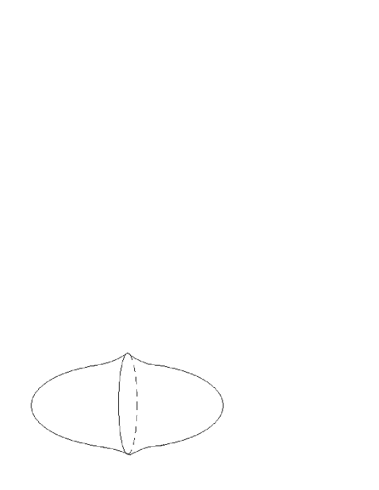
Figure 1: Configuration with a $\mathbb{Z}_{2}$-symmetric compact bulk, $\langle K_{mn}\rangle=0$, with spherical symmetry around the brane (pictured for $D=6$). The equatorial circle is the (D-1)-dimensional brane and the transverse space is compact.

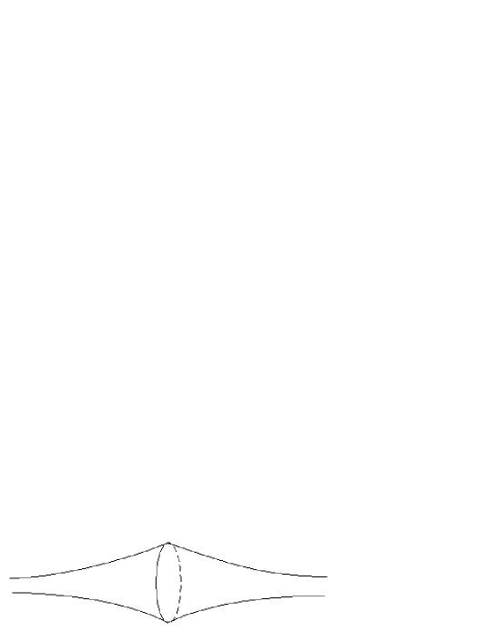
Figure 2: Configuration with a $\mathbb{Z}_{2}$-symmetric non-compact bulk, $\langle K_{mn}\rangle=0$, with spherical symmetry around the brane (pictured for $D=6$). The circle is the (D-1)-dimensional brane and the non-compact space transverse to the brane has to localize gravity.

3.2 Arbitrary number of dimensions with $\langle K_{mn}\rangle=0$

In this case there is considerably more freedom for the bulk geometry. We consider the most simple and symmetric possibility; a spherical (or axial) symmetry around the brane. The most general corresponding bulk metric can be written as

$$ds^{2}_{D}=-n^{2}(r,t)dt^{2}+a^{2}(r,t)dx^{2}_{k}+b^{2}(r,t)dr^{2}+h^{2}(r,t)r^{2}d\Omega^{2}_{D-5}\ ,$$ (3.5)

where $d\Omega^{2}$ is the $(D-5)$-dimensional sphere metric. The brane can again be assumed to sit at $r=r_{0}$, or have a trajectory $r(t)$; in any case the $(D-1)$-dimensional brane induced metric will be

$$\tilde{ds}^{2}=-d\tilde{t}^{2}+\tilde{a}^{2}(\tilde{t})dx^{2}_{k}+R^{2}(\tilde{t})d\Omega^{2}_{D-5}\ ,$$ (3.6)

where we have used coordinate freedom to use the cosmic time variable. From now on, we drop the tildes in the metric coefficients and time coordinate above. This is the product of a cosmological 4d spacetime with an internal sphere with time-dependent radius, in which matter is allowed to propagate, as is familiar from traditional Kaluza-Klein cosmology [48, 49, 50, 51].

We now show, using the same reasoning as in $D=5$, why dark radiation is no longer uniquely defined from the assumption of 3d homogeneity and isotropy, and not even after assuming spherical symmetry around the brane. All the independent contracted Bianchi identities resulting from (3.1) have been collected in the appendix. In particular, the $r0r$ component reads

$$\nabla_{e}C_{r0}^{\ \ re}=\left(\partial_{0}+3\frac{\dot{a}}{a}\right)C_{r0}^{\ \ r0}+\frac{a^{\prime}}{a}C_{0k}^{\ \ rk}+\frac{1}{r}C_{0K}^{\ \ rK}-\frac{\dot{a}}{a}C_{rk}^{\ \ rk}=0\ ,$$ (3.7)

when the bulk energy-momentum is covariantly constant, producing no right-hand side (except a singular distribution on the brane, omitted here). Using total tracelessness, this becomes

$$\left(\partial_{0}+4\frac{\dot{a}}{a}\right)E^{0}_{\ 0}=\left(\frac{a^{\prime}}{a}-\frac{1}{r}\right)C_{0K}^{\ \ rK}-\frac{\dot{a}}{a}E^{K}_{\ K}\ ,$$ (3.8)

where $K$ spans hypersphere indices. The previously unique $1/a^{4}$ behavior is manifestly spoiled by the presence of additional dimensions beyond the fifth, which now require solving for other components of the Weyl tensor in the bulk.

Taking into account these symmetries, the energy-momentum tensors can be written as

$$\tau^{m}_{\ n} = {\rm diag}(-\rho,p^{x}\ \delta^{i}_{\ j}\ ,p^{\theta}\ \delta^{I}_{\ J})$$

$$-\frac{1}{8\pi G_{D}}\langle E^{m}_{\ n}\rangle = {\rm diag}(-\rho_{d},p^{x}_{d}\ \delta^{i}_{\ j}\ ,p^{\theta}_{d}\ \delta^{I}_{\ J})$$

$$\langle{\bf T}^{a}_{\ b}\rangle = {\rm diag}(-\rho_{B},p^{x}_{B}\ \delta^{i}_{\ j},p^{\theta}_{B}\ \delta^{I}_{\ J},p^{r}_{B})+(p^{r}_{0})_{B}\delta^{a}_{\ r}\delta_{b}^{\ 0}+(p^{0}_{r})_{B}\delta^{a}_{\ 0}\delta_{b}^{\ r}\ ,$$ (3.9)

where $i,j=1..3$ denote the 3-space indices and $I,J$ the hypersphere angle indices. In addition, the dark radiation satisfies

$$\rho_{d}=3(p_{x})_{d}+(D-5)(p_{\theta})_{d}\ .$$ (3.10)

The dark radiation conservation equation (2.16) for a pure cosmological constant in the bulk is now

$$\dot{\rho}_{d}+3\frac{\dot{a}}{a}\Big{(}\rho_{d} + (p_{x})_{d}\Big{)}+(D-5)\frac{\dot{R}}{R}\Big{(}\rho_{d}+(p_{\theta})_{d}\Big{)}$$ (3.11)

$$= 8\pi G_{D}\frac{3}{4}\frac{D-5}{D-2}(p_{x}-p_{\theta})\Big{(}\dot{p}_{x}+\frac{\dot{a}}{a}(\rho+p_{x})-\dot{p}_{\theta}-\frac{\dot{R}}{R}(\rho+p_{\theta})\Big{)}\ .$$

This is a new result for $D>5$ brane cosmology: at the homogeneous background level, dark radiation is no longer conserved. Brane energy-momentum is conserved in the higher-dimensional sense, up to a jump term for the bulk energy flux:

$$\dot{\rho}+3\frac{\dot{a}}{a}(\rho+p_{x})+(D-5)\frac{\dot{R}}{R}(\rho+p_{\theta})=-[[(p^{r}_{0})_{B}]]\ n_{r}.$$ (3.12)

Assuming first that $\langle K_{mn}\rangle=0$ on the brane (see figures 1 and 2), the effective Einstein equations are:

$00$-component:

$$3\left(\frac{\dot{a}}{a}\right)^{2}+3\frac{k_{x}}{a^{2}}+(D-5)\Big{[}3\frac{\dot{R}}{R}\frac{\dot{a}}{a}+\frac{D-6}{2}\left(\frac{\dot{R}}{R}\right)^{2}+\frac{D-6}{2}\frac{k_{\theta}}{R^{2}}\Big{]}$$ (3.13)

$$= 8\pi G_{D}\frac{D-3}{D-1}{\bf\Lambda}+\frac{(8\pi G_{D})^{2}}{8}\frac{D-3}{D-2}\lambda^{2}$$

$$+8\pi G_{D}\frac{D-3}{D-2}\Big{[}\rho_{B}-\frac{D-2}{D-1}p^{r}_{B}+\frac{1}{D-1}(-\rho_{B}+3p^{x}_{B}+(D-5)p^{\theta}_{B})\Big{]}$$

$$+8\pi G_{D}\ \rho_{d}+\frac{(8\pi G_{D})^{2}}{4}\frac{D-3}{D-2}\ \lambda\ \rho$$

$$+\frac{1}{8}(8\pi G_{D})^{2}\frac{D-3}{D-2}\Big{(}\rho^{2}-3\frac{D-5}{D-3}(p_{x}-p_{\theta})^{2}\Big{)}\ ,$$

$xx$-component:

$$2\frac{\ddot{a}}{a}+\left(\frac{\dot{a}}{a}\right)^{2}+\frac{k_{x}}{a^{2}}+(D-5)\Big{[}2\frac{\dot{R}}{R}\frac{\dot{a}}{a}+\frac{D-6}{2}\left(\frac{\dot{R}}{R}\right)^{2}+\frac{D-6}{2}\frac{k_{\theta}}{R^{2}}+\frac{\ddot{R}}{R}\Big{]}$$ (3.14)

$$= 8\pi G_{D}\frac{D-3}{D-1}{\bf\Lambda}+\frac{(8\pi G_{D})^{2}}{8}\frac{D-3}{D-2}\lambda^{2}$$

$$-8\pi G_{D}\frac{D-3}{D-2}\Big{(}p^{x}_{B}+\frac{D-2}{D-1}p^{r}_{B}-\frac{1}{D-1}[-\rho_{B}+3p^{x}_{B}+(D-5)p^{\theta}_{B}]\Big{)}$$

$$-8\pi G_{D}\ p^{x}_{d}-\frac{(8\pi G_{D})^{2}}{4}\frac{D-3}{D-2}\ \lambda\ p_{x}$$

$$-\frac{1}{8}(8\pi G_{D})^{2}\frac{D-3}{D-2}\Big{(}\rho^{2}+2\rho\ p_{x}+2\frac{D-5}{D-3}(p_{\theta}-p_{x})[\rho+p_{x}+\frac{3}{2}(p_{\theta}-p_{x})]\Big{)}$$

$\theta\theta$-component:

$$3\frac{\ddot{a}}{a}+3\left(\frac{\dot{a}}{a}\right)^{2}+3\frac{k_{x}}{a^{2}}+(D-6)\Big{[}\frac{D-7}{2}\left(\frac{\dot{R}}{R}\right)^{2}+\frac{D-7}{2}\frac{k_{\theta}}{R^{2}}+3\frac{\dot{a}}{a}\frac{\dot{R}}{R}+\frac{\ddot{R}}{R}\Big{]}$$ (3.15)

$$= 8\pi G_{D}\frac{D-3}{D-1}{\bf\Lambda}+\frac{(8\pi G_{D})^{2}}{8}\frac{D-3}{D-2}\lambda^{2}$$

$$-8\pi G_{D}\frac{D-3}{D-2}\Big{(}p^{\theta}_{B}+\frac{D-2}{D-1}p^{r}_{B}-\frac{1}{D-1}[-\rho_{B}+3p^{x}_{B}+(D-5)p^{\theta}_{B}]\Big{)}$$

$$-8\pi G_{D}\ p^{\theta}_{d}-\frac{(8\pi G_{D})^{2}}{4}\frac{D-3}{D-2}\ \lambda\ p_{\theta}$$

$$-\frac{1}{8}(8\pi G_{D})^{2}\frac{D-3}{D-2}\Big{(}\rho^{2}+2\rho\ p_{x}+\frac{p_{\theta}-p_{x}}{D-3}[2(D-6)\rho-6p_{x}+3(D-7)(p_{\theta}-p_{x})]\Big{)}$$

Again, $\lambda$ and ${\bf\Lambda}$ are respectively the brane and bulk cosmological constants defined in (2.12), $k_{x}$ is the 3-space curvature parameter, and $k_{\theta}>0$ similarly for the hypersphere.

The effective Newton constant and cosmological constant on the brane are thus given by

$$8\pi G_{D-1} = \frac{1}{4}\frac{D-3}{D-2}\ \lambda\ (8\pi G_{D})^{2}$$

$$\Lambda_{D-1} = \frac{4}{8\pi G_{D}}\frac{D-2}{D-1}\frac{{\bf\Lambda}}{\lambda}+\frac{\lambda}{2}\ .$$ (3.16)

The cancellation of $\Lambda_{D-1}$ for large brane tension $\lambda$ of either sign requires a large negative ${\bf\Lambda}<0$, while positivity of $G_{D-1}$ requires a positive brane tension $\lambda>0$, as in the $D=5$ case. Note that recovering the 4d effective Newton and cosmological constants requires an additional time-dependent factor - the volume ${{\cal S}(R)}$ of the (D-5)-dimensional sphere:

$$8\pi G_{4}(t) = \frac{8\pi G_{D-1}}{{\cal S}(R)}$$

$$\Lambda_{4}(t) = \Lambda_{D-1}{\cal S}(R).$$ (3.17)

Although the product $8\pi G_{4}(t)\Lambda_{4}(t)=8\pi G_{D-1}\Lambda_{D-1}$ seems then time-independent, it must be remembered that we are not in the Einstein frame (E.F.) here, the 4d effective Newton constant being $R-$dependent. One has actually $\Lambda_{4}^{E.F.}\sim({\cal S}(R))^{-1}$, unlike a real cosmological constant source.

3.3 Arbitrary number of dimensions with $\langle K_{mn}\rangle\neq 0$

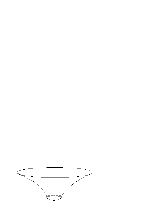
Figure 3: Natural configuration with no $\mathbb{Z}_{2}$ symmetry, $\langle K_{mn}\rangle\neq 0$, and spherical symmetry around the brane (pictured for $D=6$). The smaller circle is the (D-1)-dimensional brane. The bulk space encompassed by the brane is compact, while the outer space is non compact and has to localize gravity. The codimension one brane may be considered as a fat core regularization of a codimension (D-4) singular brane.

The assumption of vanishing average extrinsic curvature on the brane is rather unnatural for $D>5$. It implies configurations such as those depicted in figure 1 or 2, but forbids the more natural configuration of figure 3 where the brane can be considered as located approximately at the origin of the spherical coordinate system. In this last case is useful to consider the codimension one brane as a regularization of a codimension (D-4) singular brane. Furthermore, a $D-$dimensional Minkowski bulk, described by $n=a=b=h=1$ and $k=0$ in (3.5), would have a non-vanishing $\langle K^{I}_{\ J}\rangle=-\frac{1}{r}\delta^{I}_{\ J}$ in directions tangent to the hypersphere. Thus, in general we must include contributions from non-zero $\langle K_{mn}\rangle$ on the right-hand sides of (3.13-3.15). Such terms are a rational fraction of the brane energy-momentum, and quadratic in the jump of the bulk energy-momentum and Weyl tensors. The full expression being rather complicated, we provide for simplicity only the first terms in a series expansion in the variable $\rho/\lambda$ ($p_{x}$ and $p_{\theta}$ being of the same order as $\rho$). We assume also a simple form for the jump

$$\left[\left[\frac{1}{8\pi G_{D}}E^{m}_{\ n}-\frac{D-3}{D-2}\ \Big{(}{\bf T}^{a}_{\ b}\ \tilde{g}^{m}_{\ a}\ \tilde{g}^{b}_{\ n}-\frac{1}{D-1}\ \tilde{g}^{m}_{\ n}\ {\bf T}^{a}_{\ b}\ \tilde{g}^{b}_{\ a}\Big{)}-\frac{D-3}{D-1}\ \Big{(}{\bf T}^{a}_{\ b}\ n_{a}\ n^{b}\ \Big{)}\ \tilde{g}^{m}_{\ n}\ \right]\right]$$

$$=\Delta\ \tilde{g}^{m}_{\ n}\ ,$$ (3.18)

which may be realized, for example, if $[[E^{m}_{\ n}]]=0$ and the bulk content consists only of cosmological constants with different values on each side of the brane. The new contributions are then

$$-\tilde{G}^{0}_{\ 0} \supset \frac{1}{2}\frac{D-2}{(D-3)^{2}}\frac{\Delta^{2}}{\lambda^{2}}\Big{[}1-2\frac{\rho}{\lambda}-\frac{3}{\lambda^{2}}\Big{(}3(D-5)(p_{x}-p_{\theta})^{2}-(D-3)\rho^{2}\Big{)}+O(\rho^{3}/\lambda^{3})\Big{]}$$

$$-\tilde{G}^{x}_{\ x} \supset \frac{1}{2}\frac{D-2}{(D-3)^{2}}\frac{\Delta^{2}}{\lambda^{2}}\Big{[}1+2\frac{p_{x}}{\lambda}-\frac{3}{\lambda^{2}}\Big{(}(D-5)(-4p_{x}p_{\theta}+3p_{\theta}^{2}+p_{x}^{2}+2\rho p_{\theta}+\rho^{2})$$

$$+2\rho p_{x}+2\rho^{2}\Big{)}+O(\rho^{3}/\lambda^{3})\Big{]}$$

$$-\tilde{G}^{\theta}_{\ \theta} \supset \frac{1}{2}\frac{D-2}{(D-3)^{2}}\frac{\Delta^{2}}{\lambda^{2}}\Big{[}1+2\frac{p_{\theta}}{\lambda}-\frac{3}{\lambda^{2}}\Big{(}-3(D+1)p_{\theta}^{2}+(D-3)\rho^{2}+3(D-5)p_{x}^{2}$$ (3.19)

$$+18p_{x}p_{\theta}+6\rho(p_{x}-p_{\theta})\Big{)}+O(\rho^{3}/\lambda^{3})\Big{]}\ .$$

Note that the contribution linear in $\tau^{m}_{\ n}$ again has the correct tensor structure $\tilde{G}^{m}_{\ n}\supset\tau^{m}_{\ n}$ with no $(\tau\tilde{g}^{m}_{\ n})$ contribution.

3.4 Evolution of the sources

Following traditional Kaluza-Klein cosmology [48, 49, 50, 51], three simple cases may be considered for the equations of state. In the early radiation era or decompactification regime, for large temperature $T\gg 1/R$, incoherent radiation is not sensitive to the compactness of the internal space and is fully isotropic:

$$p_{\theta}=p_{x}=\frac{1}{D-2}\rho\ .$$ (3.20)

The brane energy density then evolves according to

$$\rho\sim\left(\frac{1}{a^{3}R^{D-5}}\right)^{\frac{D-1}{D-2}}\ ,$$ (3.21)

which reproduces a $1/a^{4}$ behavior for $D=5$, in the absence of an internal space.

In the late radiation era, for $T\ll 1/R$, but before matter-radiation equality, the temperature is no longer sufficient to excite an incoherent mixture of Kaluza-Klein modes on the hypersphere, so that the transverse pressure drops ($p_{\theta}=0$). Consequently $p_{x}=\frac{1}{3}\rho$, and the evolution becomes $\rho\sim 1/(a^{4}R^{D-5})$. However, it should be noted that, due to compactification, the effective energy density will include a volume factor $\rho_{eff}\sim\rho R^{D-5}$, so that

$$\rho_{eff}\sim a^{-4}\ ,$$ (3.22)

as expected.

Finally, in the matter era, after matter-radiation equality, $p_{\theta}=p_{x}=0$, and the brane energy evolves as

$$\rho_{eff}\sim a^{-3}\ .$$ (3.23)

Interestingly, this schematic picture may also be applied to dark radiation. In the early radiation and matter eras one has $(p_{x})_{d}=(p_{\theta})_{d}$ which, according to (3.11), leads to independent conservation. The evolution is the same as that of brane energy. In the late radiation era, $p_{x}\neq p_{\theta}$ and the non-conservation equation reads

$$\partial_{t}\left(\ \rho^{eff}_{d}\ a^{3\frac{D-1}{D-2}}\ R^{\frac{D-5}{D-2}}\ \right)=-\frac{D-5}{4}\ 8\pi G_{D}\ a^{3\frac{D-1}{D-2}}R^{\frac{D-5}{D-2}}\Big{[}(\rho^{eff}_{0})^{2}\left(\frac{a_{0}}{a}\right)^{8}\Big{]}\frac{1}{{\cal S}(R)}\frac{\dot{R}}{R}\ ,$$ (3.24)

where ${\cal S}(R)\sim R^{D-5}$ is the area of the (D-5)-dimensional sphere, and $\rho_{0}^{eff}$, $a_{0}$ are the values of the effective brane energy density (not of the dark radiation) and scale factor at an arbitrary reference time. This equation is not sufficient to solve for $\rho^{eff}_{d}(a,R)$, unless one assumes an algebraic relation between the two scale factors $a$ and $R$.

3.5 An example with a non-compact orbifold bulk

We have not yet made reference to a specific bulk geometry. As we mentioned before, the effective Einstein equations given previously do not guarantee the existence of a bulk solution. In the non-compact case in particular, the bulk must lead to localized gravity: in the absence of brane matter there must exist a finite volume static solution. Unfortunately, it has been shown in [52] that for a pure cosmological constant in the bulk, a compact space encompassed by the brane and a finite support for the brane energy-momentum, no localization occurs in $D>6$. This includes the configuration of figure 3, but note that the case of figure 2 is not covered by this theorem. Therefore, for the figure 3 case, a non-trivial bulk energy-momentum content is required, which has to extend to infinity, in addition to the infinitely thin brane located at finite $r$. In the following example, even though we assume a $\mathbb{Z}_{2}$ symmetry so that localized gravity may still be possible with a trivial bulk source, we will nevertheless use a non-cosmological constant bulk source.

A simple possibility [53] is a global topological defect made of a set of $D-5$ scalar fields $\phi^{a}$ with a potential

$$V(\phi)\sim\left(\sum_{a}\phi^{a}\phi^{a}-v^{2}\right)^{2}\ ,$$ (3.25)

minimized in the “hedgehog” configuration $\phi^{a}=v\ u^{a}(\theta^{K})$, with $v$ a constant scale and $u^{a}$ the unit radial vector field. The associated hyperspherical metric is then

$$d\Omega^{2}_{D-5}=\sum_{I=1}^{D-5}\Big{(}\prod_{K=1}^{I-1}\sin^{2}\theta_{K}\Big{)}d\theta_{I}^{2}$$ (3.26)

and the corresponding energy-momentum source, isotropic in both the 3-space and in the hypersphere, is

$$8\pi G_{D}{\bf T}^{\mu}_{\ \nu} = -\frac{D-5}{D-2}\ \frac{8\pi G_{D}v^{2}}{8\pi G_{D}v^{2}-(D-6)}\ {\bf\Lambda}\ \delta^{\mu}_{\ \nu}$$

$$8\pi G_{D}{\bf T}^{r}_{\ r} = -\frac{D-5}{D-2}\ \frac{8\pi G_{D}v^{2}}{8\pi G_{D}v^{2}-(D-6)}\ {\bf\Lambda}$$

$$8\pi G_{D}{\bf T}^{I}_{\ J} = -\frac{D-7}{D-2}\ \frac{8\pi G_{D}v^{2}}{8\pi G_{D}v^{2}-(D-6)}\ {\bf\Lambda}\ \delta^{I}_{J}$$ (3.27)

in addition to the bulk cosmological constant ${\bf\Lambda}<0$. (Recall that $\mu,\nu=0..3$ and $I,J$ are hypersphere angle indices.)

For $8\pi G_{D}v^{2}>(D-6)$, the static background metric is

$$ds^{2}_{D}=\exp\Big{(}-\sqrt{\frac{-16\pi G_{D}{\bf\Lambda}}{D-2}}r\Big{)}(-dt^{2}+\delta_{ij}dx^{i}dx^{j})+dr^{2}+\frac{D-2}{-16\pi G_{D}{\bf\Lambda}}\Big{(}8\pi G_{D}v^{2}-(D-6)\Big{)}d\Omega^{2}_{D-5}\ .$$ (3.28)

As the metric coefficient of the sphere line element $d\Omega_{D-5}^{2}$ is constant and thus does not vanish at $r=0$, the topology of the (D-4)-dimensional space transverse to the 4d visible dimensions is that of a cylinder $\mathbb{R}\times S^{D-5}$ rather than $\mathbb{R}^{D-5}$. The defect is located at $r=+\infty$ in these coordinates. Forgetting the topological defect origin of this bulk source, it may be considered as the most simple generalization of a bulk cosmological constant, (dropping the requirement of D-dimensional local Lorentz invariance) obeying 4d local Lorentz invariance with (D-4)-dimensional local isotropy.

If we let $r$ extend to $-\infty$ in the metric above, localization of gravity is lost. If the brane, in the static case, is located at $r=0$, we need a warp factor decreasing exponentially as $r\rightarrow-\infty$. As is familiar from $D=5$, an adequate partially anisotropic background brane tension produces the wanted effect. To simplify, we may assume a $\mathbb{Z}_{2}$ symmetry across the brane; simply replacing $r$ with $|r|$ in the metric above. The corresponding brane tension $(\lambda_{x},\lambda_{\theta})$ is then obtained from the junction conditions:

$$\rho = -p_{x}=3\sqrt{\frac{-16\pi G_{D}{\bf\Lambda}}{D-2}}\equiv\lambda_{x}$$

$$p_{\theta} = -4\sqrt{\frac{-16\pi G_{D}{\bf\Lambda}}{D-2}}\equiv-\lambda_{\theta}\ .$$ (3.29)

Alternatively, this may be deduced from the point of view of the effective Einstein equations on the brane (3.13-3.15), by taking ${\bf\Lambda}$ plus (3.27) as the bulk source, requiring staticity ($\dot{a}=\dot{R}=0$) and flat 3-space sections ($k_{x}=0$), setting the $S^{D-5}$ radius $R$ to

$$\frac{k_{\theta}}{R^{2}}=\left(\frac{1}{D-2}\right)\frac{-16\pi G_{D}{\bf\Lambda}}{8\pi G_{D}v^{2}-(D-6)}\ ,$$ (3.30)

and solving for the corresponding brane source.

If we now temporarily restore the metric form $|r|\rightarrow r$ and let the brane move in this bulk with an equation $r(t)$, while keeping the $\mathbb{Z}_{2}$ symmetry across the brane, we obtain a cosmological solution, with induced metric

$$\tilde{ds}^{2}_{D-1}=-dT^{2}+a^{2}(T)\delta_{ij}dx^{i}dx^{j}+\frac{D-2}{-16\pi G_{D}{\bf\Lambda}}\Big{(}8\pi G_{D}v^{2}-(D-6)\Big{)}d\Omega_{D-5}^{2}\ .$$ (3.31)

Note that the radius of the internal space is not dynamical ($\dot{R}=0$), even when the brane moves in the bulk. After redefining the brane energy-momentum as a departure from the tension $\lambda_{x,\theta}$ :

$$\tau^{0}_{\ 0} \rightarrow -\lambda_{x}-\rho$$

$$\tau^{i}_{\ j} \rightarrow (-\lambda_{x}+p_{x})\delta^{i}_{\ j}$$

$$\tau^{I}_{\ J} \rightarrow (-\lambda_{\theta}+p_{\theta})\delta^{I}_{\ J}$$ (3.32)

one obtains from (3.13-3.15):

$$3\left(\frac{\dot{a}}{a}\right)^{2}\supset\frac{(8\pi G_{D})^{2}}{4(D-2)}\Big{[}(D-3)\lambda_{x}\rho+3(D-5)(\lambda_{x}-\lambda_{\theta})(p_{x}-p_{\theta})\Big{]}+O\left(\frac{\rho^{2}}{\lambda_{x,\theta}^{2}}\right)$$ (3.33)

for the part linear in the brane energy-momentum. The appearance of the pressures $p_{x}$ and $p_{\theta}$ in the Friedmann equation renders this specific configuration unrealistic; more generally, the brane effective Einstein equations do not possess the correct tensor structure. The problem is due to our expanding the brane energy-momentum around a brane tension $(\lambda_{x},\lambda_{\theta})$ that does not enjoy the full (D-2)-dimensional isotropy. Requiring this is a strong constraint on the possible configurations leading to realistic gravity. In the next section, we consider a case with fully isotropic brane tension, at the expense of dropping spherical symmetry around the brane.

Another difficulty with the previous example is that the equation of state is overconstrained:

$$p_{\theta}=f(\rho,p_{x}).$$ (3.34)

This constraint is unphysical as soon as an explicit model for the source is given, in the spirit of section 3.4. Furthermore, this problem is common to all configurations in which the brane source is described by three or more parameters (like $\rho$, $p_{x}$, $p_{\theta}$ here) while the brane induced metric has a single independent scale factor $a(t)$, and this is thus generic in models where a codimension one brane moves in a static bulk. The conclusion then, is that a setup with no overconstraint on the brane equations of state requires a non-static bulk. We will comment further on this problem is the next section.

4 Cosmology with an AdS-Schwarzschild bulk

4.1 The Flat foliation

In the previous section we assumed spherical symmetry. Although this is the most symmetric bulk geometry, it introduces the complication of having to handle a curved internal space on the brane - the (D-5)-dimensional hypersphere - which leads to difficulties in obtaining localized gravity without a non-trivial bulk source. In addition to this extra complexity, this led in the previous example to an anisotropic brane tension, implying an unrealistic effective gravity due to the wrong tensor structure of the energy-momentum on the right-hand side of the Einstein equations.

However, replacing this curved space by a flat one, such as a (D-5)-dimensional hypertorus, allows for a very simple $AdS_{D}$-Schwarzschild solution:

$$ds^{2}_{D} = -\Big{(}\frac{-2{\bf\Lambda}}{(D-1)(D-2)}r^{2}-\frac{\mu}{r^{D-3}}\Big{)}dt^{2}+\frac{dr^{2}}{\frac{-2{\bf\Lambda}}{(D-1)(D-2)}r^{2}-\frac{\mu}{r^{D-3}}}$$ (4.1)

$$+r^{2}(\delta_{ij}dx^{i}dx^{j}+\delta_{IJ}dX^{I}dX^{J})\ ,$$

with a pure cosmological constant source ${\bf\Lambda}<0$ in the bulk, and where the $X^{I}$ coordinates are toroidally compactified, $X^{I}\in[0,2\pi R_{I}]$. Time-dependence of the induced metric is generated by the brane motion $r(t)$ in this static bulk. A background brane tension

$$\lambda=\sqrt{-8\frac{D-2}{D-1}\frac{{\bf\Lambda}}{8\pi G_{D}}}$$ (4.2)

is then required by the junction conditions to cancel $\Lambda_{eff}$, in accordance with (3.16). This configuration automatically inherits localized gravity from the known $AdS_{5}$ case [9, 54].

The brane induced metric has the form

$$\tilde{ds}^{2}_{D-1}=-dT^{2}+a^{2}(T)\Big{(}\delta_{ij}dx^{i}dx^{j}+\sum_{I=1}^{D-5}R_{I}^{2}d\theta_{I}^{2}\Big{)}\ ,$$ (4.3)

with $\theta_{I}\in[0,2\pi]$. In the simplifying case of an homogeneous hypercube ($R_{I}=R_{1}\ \forall I$), the corresponding effective Einstein equations (3.13-3.15) derived in the hyperspherical case still apply, with $k_{x}=k_{\theta}=0$, vanishing bulk source except ${\bf\Lambda}$, and $R(t)=R_{1}\ a(t)$. $p_{\theta}$ is then the brane pressure in the hypercube directions. This is immediately generalized to independent radii $R_{I}$ for the hypertorus, by allowing also for independent $p_{\theta_{I}}$.

Dark radiation arises from the bulk Weyl curvature due to the bulk “black hole mass” parameter $\mu$. In the coordinate system above [39]:

$$E^{m}_{\ n}=-\frac{D-3}{2}\frac{\mu}{a^{D-1}(T)}\Big{(}\delta^{m}_{\ n}-(D-1)\delta^{m}_{\ 0}\delta_{n}^{\ 0}\Big{)}$$ (4.4)

for $m,n=0,x^{i},\theta_{I}$. For differing black hole mass parameters $\mu$ and/or cosmological constants ${\bf\Lambda}$ on each side of the brane, the extra contribution (3.19) would also appear in the effective Einstein equations.

Even in absence of dark radiation ($\mu=0$), this configuration is not viable at late times. Interestingly, this is true no matter how small the compactification radii $R_{I}$ are taken, as long as the rate of variation of the size of the compact space is the same as that of the macroscopic 3-space, $\frac{\dot{R}}{R}=\frac{\dot{a}}{a}$, which is implied by the embedding we have considered. This may be seen from the brane energy conservation equation for $\rho_{eff}=\Big{(}R_{1}a(t)\Big{)}^{D-5}\rho$:

$$\dot{\rho}_{eff}+3\frac{\dot{a}}{a}(\rho_{eff}+p_{x}^{eff})=-(D-5)\frac{\dot{a}}{a}p_{\theta}^{eff}\ .$$ (4.5)

Due to the (D-1)-dimensional local isotropy of the bulk, preserved by the brane embedding, the junctions conditions imply $p_{x}=p_{\theta}$ on the brane, as in the case considered formally in [39] where no realistic compactification was attempted. In addition to being an unphysical overconstraint on the equation of state, this leads to an unacceptably large non-conservation of energy in (4.5) compared to standard cosmology, or stated differently, an unacceptably anomalous evolution law $\rho_{eff}(t)$. This immediate observational problem may have been avoided in a bulk configuration in which a small enough $p_{\theta}\ll\rho$ is allowed. Again, this problem of a constraint on $p_{\theta}$ could be predicted from the existence of a bulk timelike Killing vector.

In any case, another immediate problem, even if a vanishing $p_{\theta}$ was possible, is the unacceptably high rate of variation of the 4d effective Newton’s constant, given here in order of magnitude by the expansion rate:

$$\left|\frac{\dot{G_{4}}}{G_{4}}\right|=\left|-(D-5)\frac{\dot{R}}{R}\right|=\left|-(D-5)\frac{\dot{a}}{a}\right|\sim 10^{-10}\ {\rm yr}^{-1}\gg O(10^{-12})\ {\rm yr}^{-1}\ ,$$ (4.6)

where we have imposed the present upper bound in particular from lunar laser ranging [55, 56]. This is a universal constraint independent of the specifics of the non-gravitational interactions. Of course, if we assume these to be the Standard Model interactions, there are even stronger constraints on the cosmological variation of the internal radius, arising in particular from bounds on the variation of the fine structure constant. In addition, at the homogeneous level this study does not capture the effects of the fluctuations of the unstabilized radion.

4.2 The Hyperspherical foliation

We may choose a different parametrization of the AdS-Schwarzschild bulk (4.1) using (D-2)-dimensional spheres:

$$ds^{2}_{D} = -\Big{(}1+\frac{-2{\bf\Lambda}}{(D-1)(D-2)}r^{2}-\frac{\mu}{r^{D-3}}\Big{)}dt^{2}+\frac{dr^{2}}{1+\frac{-2{\bf\Lambda}}{(D-1)(D-2)}r^{2}-\frac{\mu}{r^{D-3}}}$$ (4.7)

$$+r^{2}\Big{[}\sum_{I=1}^{D-5}(\prod_{K=1}^{I-1}\sin^{2}\theta_{K})d\theta_{I}^{2}+(\prod_{L=1}^{D-5}\sin^{2}\theta_{L})d\Omega_{3}^{2}\Big{]}\ ,$$

where this time $d\Omega_{3}^{2}$ is the line element of a 3-sphere representing the visible macroscopic 3-space. The brane embedding is now physically different; in particular there is now no need to compactify the transverse space induced on the brane because the total brane space is compact. The visible 3-space is now compact too. The induced metric has the form

$$\tilde{ds}^{2}_{D-1}=-dT^{2}+a^{2}(T)\Big{[}\sum_{I=1}^{D-5}\left(\prod_{K=1}^{I-1}\sin^{2}\theta_{K}\right)d\theta_{I}^{2}+\left(\prod_{L=1}^{D-5}\sin^{2}\theta_{L}\right)d\Omega_{3}^{2}\Big{]}\ .$$ (4.8)

It is obvious that, contrary to the previous case with a flat foliation, there is no freedom to make the characteristic size of the internal space much smaller than the radius of the visible 3-space. This immediately leads to a problem, since we require matter to propagate in the internal space on the brane.

5 Conclusions

In this paper, we have derived the effective Einstein equations for the cosmological evolution of a codimension one brane embedded in a general D-dimensional bulk with spherical symmetry around the brane. The geometrical side of the effective Friedmann equation corresponds to the product of a 4d cosmological spacetime with an internal sphere with time-dependent radius. When the brane tension $\lambda$ enjoys a full (D-2)-dimensional isotropy, the source side of the Friedmann equation contains the standard term linear in the brane energy plus quadratic corrections of order $O(\rho^{2}/\lambda^{2})$, in addition to terms linear in the bulk energy-momentum. When it does not, the effective gravity does not have the correct tensor structure for the part linear in the brane source. We have included contributions to the effective source arising from the breaking of the $\mathbb{Z}_{2}$ symmetry across the brane. We have shown that the bulk radiation manifests itself as an extra conformally invariant “dark radiation” source, which is in general not conserved, contrary to the $D=5$ case. By taking the example of an AdS-Schwarzschild bulk, we have illustrated the problem that any static bulk necessarily leads to an overconstraint on the brane matter equation of state.

These simple analytic examples provide a useful guide for the explicit construction of realistic cosmological metrics in the bulk in $D\geq 7$. As an alternative approach to codimension one branes, it may be interesting to derive the effective Friedmann equations in a regularization-independent way for fat branes of codimension (D-4), as a perturbation expansion in the brane energy density integrated over the core.
 

Acknowledgments

NC and MT are supported by the National Science Foundation under grant number PHY-0354990, by Research Corporation, and by funds provided by Syracuse University. NC and CM are supported by the Department of Energy, under grant number DE-FG02-85ER40231.

Appendix : Bulk contracted Bianchi identities in the cosmological case

The most general metric with cosmological symmetries and spherical symmetry around the brane (for vanishing 3-space curvature) can be written as

$$ds^{2}_{D}=-n^{2}(r,t)dt^{2}+a^{2}(r,t)\delta_{ij}dx^{i}dx^{j}+b^{2}(r,t)dr^{2}+r^{2}d\Omega^{2}_{D-5}\ ,$$ (5.1)

where it is always possible to set the $g_{IJ}$ component, proportional here to $r^{2}$, as time-independent, as long as the brane is allowed to move in the bulk. The contracted Bianchi identities read, after using Einstein equations,

$$\nabla^{e}C_{abce}=-8\pi G_{D}\frac{D-3}{D-2}\nabla_{[a}\Big{(}{\bf T}_{b]c}-\frac{1}{D-1}{\bf T}g_{b]c}\Big{)}\ .$$ (5.2)

Symmetries severely constrain the 3-index tensor on the left-hand side, leaving only six independent components (before using the extra tracelessness constraints). We write them explicitly here:

$$\nabla_{e}C_{r0}^{\ \ re} = \left(\partial_{0}+3\frac{\dot{a}}{a}\right)C_{r0}^{\ \ r0}+\frac{a^{\prime}}{a}C_{0k}^{\ \ rk}+\frac{1}{r}C_{0K}^{\ \ rK}-\frac{\dot{a}}{a}C_{rk}^{\ \ rk}$$

$$\nabla_{e}C_{0r}^{\ \ 0e} = \left(\partial_{r}+3\frac{a^{\prime}}{a}+\frac{D-5}{r}\right)C_{r0}^{\ \ r0}+\frac{\dot{a}}{a}C_{rk}^{\ \ 0k}-\frac{a^{\prime}}{a}C_{0k}^{\ \ 0k}-\frac{1}{r}C_{0I}^{\ \ 0I}$$

$$\nabla_{e}C_{i0}^{\ \ je} = \left(\partial_{0}+\frac{\dot{b}}{b}+2\frac{\dot{a}}{a}\right)C_{i0}^{\ \ j0}+\left(\partial_{r}+\frac{b^{\prime}}{b}+2\frac{a^{\prime}}{a}-\frac{n^{\prime}}{n}+\frac{D-5}{r}\right)C_{i0}^{\ \ jr}-\frac{\dot{a}}{a}C_{ik}^{\ \ jk}-\frac{\dot{b}}{b}C_{ir}^{\ \ jr}$$

$$\nabla_{e}C_{I0}^{\ \ Je} = \left(\partial_{0}+\frac{\dot{b}}{b}+3\frac{\dot{a}}{a}\right)C_{I0}^{\ \ J0}+\left(\partial_{r}+\frac{b^{\prime}}{b}+3\frac{a^{\prime}}{a}-\frac{n^{\prime}}{n}+\frac{D-6}{r}\right)C_{I0}^{\ \ Jr}-\frac{\dot{a}}{a}C_{Ik}^{\ \ Jk}-\frac{\dot{b}}{b}C_{Ir}^{\ \ Jr}$$

$$\nabla_{e}C_{ir}^{\ \ je} = \left(\partial_{0}+2\frac{\dot{a}}{a}-\frac{\dot{b}}{b}+\frac{\dot{n}}{n}\right)C_{ir}^{\ \ j0}+\left(\partial_{r}+2\frac{a^{\prime}}{a}+\frac{n^{\prime}}{n}+\frac{D-5}{r}\right)C_{ir}^{\ \ jr}-\frac{a^{\prime}}{a}C_{ik}^{\ \ jk}-\frac{1}{r}C_{iK}^{\ \ jK}$$

$$-\frac{n^{\prime}}{n}C_{i0}^{\ \ j0}$$

$$\nabla_{e}C_{Ir}^{\ \ Je} = \left(\partial_{0}+3\frac{\dot{a}}{a}+\frac{\dot{n}}{n}-\frac{\dot{b}}{b}\right)C_{Ir}^{\ \ J0}+\left(\partial_{r}+3\frac{a^{\prime}}{a}+\frac{n^{\prime}}{n}+\frac{D-5}{r}\right)C_{Ir}^{\ \ Jr}-\frac{1}{r}C_{IK}^{\ \ JK}-\frac{n^{\prime}}{n}C_{I0}^{\ \ J0}$$ (5.3)

$$-\frac{a^{\prime}}{a}C_{Ik}^{\ \ Jk}$$

where $i,j,k$ denote 3-space indices, and $I,J,K$ hypersphere angle indices.

References

• [1] T. Kaluza, Sitzungsber. Preuss. Akad. Wiss. Berlin (Math. Phys. ) 1921, 966 (1921).
• [2] O. Klein, Z. Phys.  37, 895 (1926) [Surveys High Energ. Phys.  5, 241 (1986)].
• [3] V. A. Rubakov and M. E. Shaposhnikov, Phys. Lett. B 125 (1983) 136.
• [4] I. Antoniadis, Phys. Lett. B 246, 377 (1990).
• [5] J. D. Lykken, Phys. Rev. D 54, 3693 (1996) [arXiv:hep-th/9603133].
• [6] N. Arkani-Hamed, S. Dimopoulos and G. R. Dvali, Phys. Lett. B 429, 263 (1998) [arXiv:hep-ph/9803315].
• [7] I. Antoniadis, N. Arkani-Hamed, S. Dimopoulos and G. R. Dvali, Phys. Lett. B 436, 257 (1998) [arXiv:hep-ph/9804398].
• [8] L. Randall and R. Sundrum, Phys. Rev. Lett.  83 (1999) 3370 [arXiv:hep-ph/9905221].
• [9] L. Randall and R. Sundrum, Phys. Rev. Lett.  83, 4690 (1999) [arXiv:hep-th/9906064].
• [10] J. Lykken and L. Randall, JHEP 0006, 014 (2000) [arXiv:hep-th/9908076].
• [11] N. Arkani-Hamed, S. Dimopoulos, G. R. Dvali and N. Kaloper, Phys. Rev. Lett.  84, 586 (2000) [arXiv:hep-th/9907209].
• [12] I. Antoniadis and K. Benakli, Phys. Lett. B 326, 69 (1994) [arXiv:hep-th/9310151].
• [13] K. R. Dienes, E. Dudas and T. Gherghetta, Nucl. Phys. B 537, 47 (1999) [arXiv:hep-ph/9806292].
• [14] N. Kaloper, J. March-Russell, G. D. Starkman and M. Trodden, Phys. Rev. Lett.  85, 928 (2000) [arXiv:hep-ph/0002001].
• [15] N. Arkani-Hamed, S. Dimopoulos and G. R. Dvali, Phys. Rev. D 59 (1999) 086004 [arXiv:hep-ph/9807344].
• [16] C. Macesanu and M. Trodden, Phys. Rev. D 71 (2005) 024008 [arXiv:hep-ph/0407231].
• [17] G. D. Starkman, D. Stojkovic and M. Trodden, Phys. Rev. Lett.  87, 231303 (2001) [arXiv:hep-th/0106143].
• [18] G. D. Starkman, D. Stojkovic and M. Trodden, Phys. Rev. D 63, 103511 (2001) [arXiv:hep-th/0012226].
• [19] C. Deffayet, G. R. Dvali and G. Gabadadze, arXiv:astro-ph/0106449.
• [20] C. Deffayet, G. R. Dvali and G. Gabadadze, Phys. Rev. D 65, 044023 (2002) [arXiv:astro-ph/0105068].
• [21] G. R. Dvali, G. Gabadadze and M. Porrati, Phys. Lett. B 485, 208 (2000) [arXiv:hep-th/0005016].
• [22] C. Deffayet, S. J. Landau, J. Raux, M. Zaldarriaga and P. Astier, Phys. Rev. D 66, 024019 (2002) [arXiv:astro-ph/0201164].
• [23] C. Deffayet, Phys. Lett. B 502, 199 (2001) [arXiv:hep-th/0010186].
• [24] G. Dvali and M. S. Turner, arXiv:astro-ph/0301510.
• [25] A. Lue, R. Scoccimarro and G. D. Starkman, Phys. Rev. D 69, 124015 (2004) [arXiv:astro-ph/0401515].
• [26] A. Lue and G. Starkman, Phys. Rev. D 67, 064002 (2003) [arXiv:astro-ph/0212083].
• [27] P. Binetruy, C. Deffayet, U. Ellwanger and D. Langlois, Phys. Lett. B 477, 285 (2000) [arXiv:hep-th/9910219].
• [28] P. Binetruy, C. Deffayet and D. Langlois, Nucl. Phys. B 615, 219 (2001) [arXiv:hep-th/0101234].
• [29] P. Binetruy, C. Deffayet and D. Langlois, Nucl. Phys. B 565, 269 (2000) [arXiv:hep-th/9905012].
• [30] D. J. H. Chung and K. Freese, Phys. Rev. D 61, 023511 (2000) [arXiv:hep-ph/9906542].
• [31] C. Csaki, M. Graesser, L. Randall and J. Terning, Phys. Rev. D 62 (2000) 045015 [arXiv:hep-ph/9911406].
• [32] J. M. Cline and J. Vinet, JHEP 0202 (2002) 042 [arXiv:hep-th/0201041].
• [33] S. M. Carroll and M. M. Guica, arXiv:hep-th/0302067.
• [34] I. Navarro, JCAP 0309 (2003) 004 [arXiv:hep-th/0302129].
• [35] J. Vinet and J. M. Cline, Phys. Rev. D 70 (2004) 083514 [arXiv:hep-th/0406141].
• [36] J. Vinet and J. M. Cline, Phys. Rev. D 71 (2005) 064011 [arXiv:hep-th/0501098].
• [37] B. Cuadros-Melgar and E. Papantonopoulos, Phys. Rev. D 72 (2005) 064008 [arXiv:hep-th/0502169].
• [38] K. Lanczos (1922), unpublished; Ann. Phys. (Leipzig) 74 (1924) 518; N. Sen, Ann. Phys. (Leipzig) 73 (1924) 365; G. Darmois, Mémorial des sciences mathématiques XXV (1927); W. Israel, Nuovo Cimento 44B (1966) 1, erratum: Nuovo Cimento 48B (1966) 463.
• [39] R. A. Battye, B. Carter, A. Mennim and J. P. Uzan, Phys. Rev. D 64 (2001) 124007 [arXiv:hep-th/0105091].
• [40] P. Horava and E. Witten, Nucl. Phys. B 475 (1996) 94 [arXiv:hep-th/9603142].
• [41] T. Shiromizu, K. i. Maeda and M. Sasaki, Phys. Rev. D 62 (2000) 024012 [arXiv:gr-qc/9910076].
• [42] P. Bowcock, C. Charmousis and R. Gregory, Class. Quant. Grav.  17 (2000) 4745 [arXiv:hep-th/0007177].
• [43] D. Ida, JHEP 0009 (2000) 014 [arXiv:gr-qc/9912002].
• [44] A. C. Davis, S. C. Davis, W. B. Perkins and I. R. Vernon, Phys. Lett. B 504 (2001) 254 [arXiv:hep-ph/0008132].
• [45] N. Deruelle and T. Dolezel, Phys. Rev. D 62 (2000) 103502 [arXiv:gr-qc/0004021].
• [46] W. B. Perkins, Phys. Lett. B 504 (2001) 28 [arXiv:gr-qc/0010053].
• [47] H. Stoica, S. H. H. Tye and I. Wasserman, Phys. Lett. B 482 (2000) 205 [arXiv:hep-th/0004126].
• [48] R. B. Abbott, S. M. Barr and S. D. Ellis, Phys. Rev. D 30 (1984) 720.
• [49] R. B. Abbott, S. D. Ellis and S. M. Barr, Phys. Rev. D 31 (1985) 673.
• [50] D. Sahdev, Phys. Rev. D 30 (1984) 2495.
• [51] D. Sahdev, Phys. Lett. B 137 (1984) 155.
• [52] T. Gherghetta, E. Roessl and M. E. Shaposhnikov, Phys. Lett. B 491 (2000) 353 [arXiv:hep-th/0006251].
• [53] I. Olasagasti and A. Vilenkin, Phys. Rev. D 62 (2000) 044014 [arXiv:hep-th/0003300].
• [54] R. Bao and J. D. Lykken, arXiv:hep-ph/0509137.
• [55] C. M. Will, arXiv:gr-qc/0510072.
• [56] J. G. Williams, S. G. Turyshev and D. H. Boggs, Phys. Rev. Lett.  93 (2004) 261101 [arXiv:gr-qc/0411113].