Testing the Accuracy and Stability of Spectral Methods in Numerical Relativity

Abstract

The accuracy and stability of the Caltech-Cornell pseudospectral code is evaluated using the Kidder, Scheel, and Teukolsky (KST) representation of the Einstein evolution equations. The basic “Mexico City Tests” widely adopted by the numerical relativity community are adapted here for codes based on spectral methods. Exponential convergence of the spectral code is established, apparently limited only by numerical roundoff error or by truncation error in the time integration. A general expression for the growth of errors due to finite machine precision is derived, and it is shown that this limit is achieved here for the linear plane-wave test.

I Introduction

A number of groups have now developed numerical relativity codes sophisticated enough to evolve binary black-hole spacetimes Pretorius (2005); Baker et al. (2006); Campanelli et al. (2006); Diener et al. (2006); Herrmann et al. (2006); Scheel et al. (2006). The gravitational waveforms predicted by these evolutions will play an important role in detecting and interpreting the physical properties of the sources of these waves soon to be detected (we presume) by the community of gravitational wave observers (e.g., LIGO, etc.). Therefore, such codes must be capable of performing stable and accurate simulations of very nonlinear and dynamical spacetimes.

Several years ago a large subset of the numerical relativity community, the “Apples with Apples” collaboration Alcubierre et al. (2004), proposed a series of basic code tests designed to verify the accuracy, stability, robustness and efficiency of any code designed to find fully three-dimensional solutions to the Einstein evolution equations. These tests—often referred to as the “Mexico City Tests” because they were first formulated during a conference in Mexico City in May 2002—were designed to be analogous to the standard suite of tests used by the numerical hydrodynamics community (e.g., tests to reproduce Sedov explosions, Sod shock tubes, blast waves, etc.) to commission new hydrodynamics codes. The Mexico City tests were designed to be applicable to any formulation of Einstein’s equations solved with any numerical method. All tests proposed so far concern bulk properties of the formulation and numerical method, and so all of the evolutions are carried out on a numerical grid with three-torus topology; no boundary conditions are needed (or tested). There are four basic tests, some of them in a number of variations: (a) the evolution of certain “random” initial data; (b) the evolution of small-amplitude “linear” plane-wave initial data; (c) the evolution of a nonlinear gauge-wave representation of flat spacetime; and (d) the evolution of initial data for a very dynamic and nonlinear Gowdy cosmological model.

The Mexico City tests have now been applied to a number of different numerical relativity codes that use different formulations of the Einstein equations Alcubierre et al. (2004); Jansen et al. (2006). But all of the codes tested so far use finite difference numerical methods. In this paper we report the results of applying these tests to the code being developed by the collaboration between the Caltech and Cornell numerical relativity groups. We use a first-order symmetric-hyperbolic formulation of the equations developed by Kidder, Scheel and Teukolsky Kidder et al. (2001) (sometimes referred to as the KST formulation) and we solve the equations using pseudospectral numerical methods. The results reported here differ therefore from all previously tested cases both in the formulation of the Einstein equations and the numerical methods used to solve them.

This paper is organized as follows: In Sec. II we review the KST formulation of the equations and the pseudospectral numerical methods that we use to solve them. The remaining sections present the results of the various Mexico City tests, adapted somewhat to provide more challenging tests of a code based on spectral methods. In Sec. III we show that our code is stable when evolving small random perturbations of flat spacetime. In Sec. IV we report the results of the small-amplitude plane-wave test. We demonstrate the convergence rates for different spatial resolutions and different time-step algorithms. We also derive an equation for the error introduced by finite machine precision, and show that it limits the convergence of our evolutions for small spatial and temporal resolutions. In Sec. V we show the stability of our evolution code for nonlinear gauge waves. In this case, nonlinear terms give rise to an instability that is drastically reduced by suitably filtering the components of the spectral expansion. Section VI shows the performance of our code for evolutions of the highly dynamical Gowdy spacetime, in which the exact analytical expressions for the components of the fields grow exponentially in time. Finally, we discuss and summarize our various results in Sec. VII.

II Solution Method

In this section we describe the formulation of the Einstein equations and the pseudospectral numerical solution method that we test. The Mexico City tests were designed with finite-difference methods in mind and were originally applied to formulations of the Einstein equations that are second-order in space and first-order in time. Both our numerical methods and our representation of the Einstein equations differ significantly from those in Ref. Alcubierre et al. (2004), so appropriate modifications to the Mexico City test suite (for example, the number of grid points used or the constraint quantities observed) are needed. These modifications are also described in this section.

II.1 KST Formulation

The KST system Kidder et al. (2001) is a first-order symmetric hyperbolic generalization of York’s representation of the ADM equations York (1979). The dynamical variables of this system are the three-metric $g_{ij}$, the extrinsic curvature $K_{ij}$, and a new variable $D_{kij}$ that is initially set equal to $\partial_{k}g_{ij}/2$. This last variable allows the system to be put into first-order form. Its introduction results in two additional constraints:

$$C_{kij} \equiv D_{kij}-\frac{1}{2}\,\partial_{k}g_{ij}\ ,$$ (1)

$$C_{lkij} \equiv\partial_{[l}D_{k]ij}\ .$$ (2)

The KST evolution equations are obtained from the ADM equations York (1979) by adding constant multiples of the various constraints to the evolution equations and by replacing the lapse with a lapse density function. These changes do not affect the physical solutions of the system, but they do modify the unphysical constraint-violating solutions. The added constraint terms are proportional to constant parameters $\left\{\gamma_{1},\gamma_{2},\gamma_{3},\gamma_{4}\right\}$, which are chosen to make the system symmetric hyperbolic Kidder et al. (2005). The principal parts of the KST evolution equations, then, are given by:

$$\partial_{t}g_{ij} \simeq N^{n}\partial_{n}g_{ij}\ ;$$ (3)

$$\partial_{t}K_{ij} \simeq N^{n}\partial_{n}K_{ij}-N\Bigl{[}(1+2\gamma_{0})g^{cd}\delta^{n}_{\phantom{n}(i}\delta^{b}_{\phantom{b}j)}$$ (4)

$$-(1+\gamma_{2})g^{nd}\delta^{b}_{\phantom{b}(i}\delta^{c}_{\phantom{c}j)}-(1-\gamma_{2})g^{bc}\delta^{n}_{\phantom{n}(i}\delta^{d}_{\phantom{d}j)}$$

$$+g^{nb}\delta^{c}_{\phantom{c}i}\delta^{d}_{\phantom{d}j}+2\gamma_{1}g{}^{n[b}g{}^{d]c}g{}_{ij}\Bigr{]}\partial_{n}D_{bcd}\ ;$$

$$\partial_{t}D_{kij} \simeq N^{n}\partial_{n}D_{kij}-N\Bigl{[}\delta^{n}_{\phantom{n}k}\delta^{b}_{\phantom{k}i}\delta^{c}_{\phantom{j}j}-\frac{1}{2}\,\gamma_{3}g^{nb}g_{k(i}\delta^{c}_{\phantom{c}j)}$$ (5)

$$-\frac{1}{2}\,\gamma_{4}g{}^{nb}g{}_{ij}\delta{}^{c}{}_{k}+\frac{1}{2}\,\gamma_{3}g{}^{bc}g{}_{k(i}\delta{}^{n}{}_{j)}$$

$$+\frac{1}{2}\,\gamma_{4}g{}^{bc}g{}_{ij}\delta{}^{n}{}_{k}\Bigr{]}\partial_{n}K_{bc}\ .$$

Here, the symbol $\simeq$ indicates that terms algebraic in the fields (that is, nonprincipal terms) are not shown explicitly. The lapse function $N$ is taken to be

$$N\equiv g^{\gamma_{0}}e^{Q}\ ,$$ (6)

and both the lapse density function $Q$ and the shift $N^{i}$ are assumed to be specified functions of the coordinates, rather than independent dynamical fields. Since each of the Mexico City tests involves reproducing either a known analytic solution of the Einstein equations or a small perturbation about a known solution, for all tests reported here we set the lapse density $Q$ and the shift $N^{i}$ from the appropriate analytic solution. We choose one set of the KST parameters for all the tests here: $\gamma_{0}=0.5$; $\gamma_{1}=-0.21232$; $\gamma_{2}=-0.00787402$; $\gamma_{3}=-1.61994$; $\gamma_{4}=-0.69885$. These values were chosen because they make the KST system symmetric hyperbolic and coincide with a set preferred by Owen Owen (2006) in his extension of the KST system.

To evaluate errors it is useful to look at constraint quantities. As mentioned above, the KST system has additional constraints, Eqs. (1) and (2), besides the usual Hamiltonian constraint $C$ and momentum constraint $C_{i}$. To ensure that we are satisfying all the constraints, we monitor a single quantity $\mathcal{C}$ that is zero if and only if all of the constraints vanish:

$$\mathcal{C}\equiv\sqrt{C^{2}+\left(C_{i}\right)^{2}+\left(C_{kij}\right)^{2}+\left(C_{lkij}\right)^{2}}\ ,$$ (7)

where an object is squared using the evolved spatial metric: for example, $(C_{i})^{2}=g^{ij}C_{i}C_{j}$.

Likewise, when evaluating differences from analytically known solutions, we define an overall error quantity that includes the errors in all evolved variables $g_{ij}$, $K_{ij}$, and $D_{kij}$. Taking $\delta g_{ij}\equiv g_{ij}^{\mathrm{analytic}}-g_{ij}^{\mathrm{evolved}}$, and similarly for other fundamental fields, this overall error quantity is given by

$$\delta\,\mathcal{U} \equiv \sqrt{\left(\delta g_{ij}\right)^{2}+\left(\delta K_{ij}\right)^{2}+\left(\delta D_{kij}\right)^{2}}\ .$$ (8)

Notice that $\delta\,\mathcal{U}$ vanishes if and only if all evolved variables match the known solution.

For all error quantities $\mathcal{Q}$ we display $L_{2}$ norms:

$$\left\|\mathcal{Q}\right\|_{2}\equiv\sqrt{\frac{1}{\mathrm{Vol}}\,\int\,\mathcal{Q}^{2}\,\sqrt{|g|}\,d^{3}x}\ ,$$ (9)

where $\mathrm{Vol}=\int\sqrt{|g|}d^{3}x$ is the volume of the domain. These norms are computed after each time step over the current $t=\mbox{const.}$ hypersurface. We refer to $\|\mathcal{C}\|_{2}$ as the constraint energy, and $\|\delta\,\mathcal{U}\|_{2}$ as the error energy.

The error quantities $\|\delta\,\mathcal{U}\|_{2}$ and $\|\mathcal{C}\|_{2}$ scale with the absolute magnitude of the fundamental fields and their derivatives, so it can be difficult to judge the significance of these error measures without knowing the overall scale of the variables in the problem. For this reason, we sometimes plot the normalized error energy $\|\delta\,\mathcal{U}\|_{2}/\|\mathcal{U}\|_{2}$ and the normalized constraint energy $\|\mathcal{C}\|_{2}/\|\partial\,\mathcal{U}\|_{2}$, where the normalization factors are defined by

$$\mathcal{U} \equiv \sqrt{\left(g_{ij}\right)^{2}+\left(K_{ij}\right)^{2}+\left(D_{kij}\right)^{2}}\ ,$$ (10)

$$\partial\,\mathcal{U} \equiv \sqrt{\left(\partial_{i}g_{jk}\right)^{2}+\left(\partial_{i}K_{jk}\right)^{2}+\left(\partial_{i}D_{jkl}\right)^{2}}\ .$$ (11)

Note that $\|\delta\,\mathcal{U}\|_{2}/\|\mathcal{U}\|_{2}$ and $\|\mathcal{C}\|_{2}/\|\partial\,\mathcal{U}\|_{2}$ become of order unity when errors completely dominate the numerical solution. We display normalized error quantities only for tests involving the Gowdy spacetimes (Section VI), in which the fundamental variables vary exponentially in time. All other tests presented here involve perturbations of Minkowski spacetime, in which case the quantity $\|\partial\,\mathcal{U}\|_{2}$ is of order the size of the perturbation and is therefore inappropriate to use as a normalization factor. However, for perturbations of Minkowski spacetime, the overall scale is of order unity so it suffices to display the unnormalized quantities $\|\delta\,\mathcal{U}\|_{2}$ and $\|\mathcal{C}\|_{2}$.

II.2 Pseudospectral Methods

All of our numerical computations are carried out using pseudospectral methods; this is the first time the Mexico City tests have been applied to a pseudospectral code. A brief outline of our method is as follows: Given a system of partial differential equations

$$\partial_{t}u(\mathbf{x},t)=\mathcal{F}[u(\mathbf{x},t),\partial_{i}u(\mathbf{x},t)]\ ,$$ (12)

where $u$ is a collection of dynamical fields, the solution $u(\mathbf{x},t)$ is expressed as a time-dependent linear combination of $N$ spatial basis functions $\phi_{k}(\mathbf{x})$:

$$u(\mathbf{x},t)=\sum_{k=0}^{N-1}\tilde{u}_{k}(t)\phi_{k}(\mathbf{x})\ .$$ (13)

Associated with the basis functions is a set of $N_{c}$ collocation points $\mathbf{x}_{i}$. Given spectral coefficients $\tilde{u}_{k}(t)$, the function values at the collocation points $u(\mathbf{x}_{i},t)$ are computed using Eq. (13). Conversely, the spectral coefficients are obtained by the inverse transform

$$\tilde{u}_{k}(t)=\sum_{i=0}^{N_{c}-1}w_{i}u(\mathbf{x}_{i},t)\phi_{k}(\mathbf{x}_{i})\ ,$$ (14)

where $w_{i}$ are weights specific to the choice of basis functions and collocation points. Thus it is straightforward to transform between the spectral coefficients $\tilde{u}_{k}(t)$ and the function values at the collocation points $u(\mathbf{x}_{i},t)$.

To solve the differential equations, we evaluate spatial derivatives analytically using the known derivatives of the basis functions,

$$\partial_{i}u(\mathbf{x},t)=\sum_{k=0}^{N-1}\tilde{u}_{k}(t)\partial_{i}\phi_{k}(\mathbf{x})\ ,$$ (15)

and we evaluate nonlinear terms using the values of $u(\mathbf{x}_{i},t)$ at the collocation points. Thus we can write the partial differential equation, Eq. (12), as a set of ordinary differential equations for the function values at the collocation points,

$$\partial_{t}u(\mathbf{x}_{i},t)=\mathcal{G}_{i}[u(\mathbf{x}_{j},t)]\ ,$$ (16)

where $\mathcal{G}_{i}$ depends on $u(\mathbf{x}_{j},t)$ for all $j$. We then integrate this system of ordinary differential equations in time, using (for example) a fourth-order Runge-Kutta algorithm.

Because the tests discussed here are periodic in all spatial dimensions, we use Fourier basis functions. If we choose a computational domain extending from $-1/2$ to $1/2$ in each of the $x$-, $y$-, and $z$-directions, then each variable $u$ is decomposed as

$$u(x,y,z)=\sum_{k=0}^{N_{x}-1}\,\sum_{l=0}^{N_{y}-1}\,\sum_{m=0}^{N_{z}-1}\,a_{klm}\phi_{k}(x)\phi_{l}(y)\phi_{m}(z),$$ (17)

where

$$\phi_{k}(x)=\left\{\begin{array}[]{ll}1&k=0\ ;\\ \sin[\pi x(k+1)]&k>0\ \ (k\mathrm{~{}odd})\ ;\\ \cos(\pi xk)&k>0\ \ (k\mathrm{~{}even})\ .\end{array}\right.$$ (18)

For smooth solutions, the spectral approximation Eq. (13) converges exponentially (error $\sim e^{-\lambda N}$ for some $\lambda>0$ which depends on the solution). This is much faster than the polynomial convergence (error $\sim 1/N^{p}$) obtained using $p$th-order finite-differencing. As a result, we run our tests at coarser resolutions than those recommended in Ref. Alcubierre et al. (2004) for finite-difference codes—typically we use $N_{i}=9$, 15, 21, 27, and 33 collocation points in the relevant directions. From Eqs. (17) and (18) we see that if we choose $N_{x}$, $N_{y}$, or $N_{z}$ to be an even integer, the highest frequency component in our expansion will have a sine term but no matching cosine term. Consequently the spatial derivative of this highest frequency component will not be represented by our basis functions, causing a numerical instability. Therefore we choose $N_{x}$, $N_{y}$, and $N_{z}$ to be odd.

Because spectral methods so greatly reduce spatial discretization errors, time-stepping error is often dominant. In order to make the time stepping and the spatial discretization errors comparable in these tests, we use fourth-order Runge-Kutta ODE integration. The time-step sizes are chosen in an effort to use step sizes comparable to those used to test finite difference methods in Ref. Alcubierre et al. (2004), while also ensuring that time-step errors do not dominate over our spatial truncation errors. We use $\Delta t=\Delta x/20$ in the first test, and $\Delta t=\Delta x/40$ in all others, except where explicitly noted. Here, $\Delta x$ is the minimum distance between collocation points.

III Random Initial Data on Flat Space

Perhaps the simplest test of a numerical relativity code is evolving standard Minkowski spacetime on a three-torus, $T^{3}$. However, this test is too simple because all fundamental fields are spatially constant and most are identically zero, and hence most numerical methods will reproduce the correct solution exactly. This test can be made more discriminating by adding a small amount of random noise to the initial data; the noise is intended to simulate the effect of finite numerical precision. A different random number is added to each component of each evolved variable, at each point in the domain. These random numbers are chosen to lie between $-10^{-10}$ and $10^{-10}$ so that the system remains in the linear regime. If these small perturbations to a simple spacetime grow unstably, it is likely that the inevitable errors (e.g., discretization error or even numerical roundoff error) that arise in any more complicated simulation will also grow unstably. For this test we vary the resolution in the $x$-dimension, and we fix the resolution to three collocation points in each of the $y$- and $z$-dimensions.

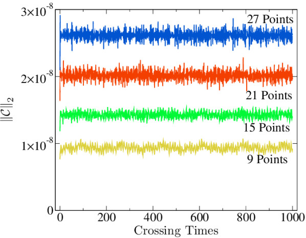
Figure 1: Constraints for Minkowski with Random Noise. Higher resolutions are expected to have larger constraints because more closely spaced points result in larger derivatives. The constraints do not grow in time.

If the perturbations in the fields are chosen to be of size $\epsilon$ independent of resolution, then the perturbation in the $n$th spatial derivatives of these fields will be $\sim\epsilon(\Delta x)^{-n}$, where $\Delta x$ is some measure of the distance between neighboring points. This means that error quantities involving derivatives (such as constraints) will be larger for finer resolutions. This behavior is seen in the plot of the constraint energy in Fig. 1.

The purpose of this test is to establish that small constraint violations around flat space do not grow, and the KST system clearly passes this test. Whether or not constraint violations decay will depend on the evolution system and the numerical method. For example, artificial dissipation in the numerical method might cause all variations to decay, including constraint violations. Furthermore, if the evolution system contains constraint damping in some form, then the constraints should decay. Indeed, Owen has extended the KST system to include constraint damping Owen (2006); running the same test, he observes exponential decay in the constraint quantities. The flat constraint violations observed in Fig. 1 indicate that the KST system with our parameter choice does not damp constraints and that the spectral method has insignificant artificial dissipation.

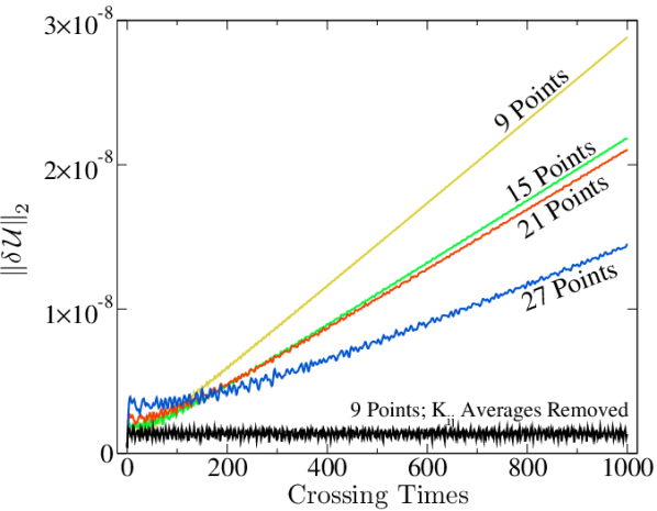
Figure 2: Error Energy for Minkowski with Random Noise. The linear increase in time is due to a nonzero average in the random noise added to $K_{ij}$. This average approaches zero as resolution is increased, since there are more points over which to average. The flat line shows the evolution when the average value of $K_{ij}$ is set to zero in the initial data.

In Fig. 2 we see a linear growth of the error energy $\|\delta\,\mathcal{U}\|$ for this test. We find that the growth is caused solely by contributions from the metric $g_{ij}$; the average values of $K_{ij}$ and $D_{kij}$ remain constant in time. We can understand this as follows: The average value of $K_{ij}$ is determined by the random initial data and will in general be nonzero. The time derivative of $K_{ij}$, to first order in the amplitude of perturbations around flat space, involves only spatial derivatives of $D_{kij}$. These derivatives have zero average (up to roundoff errors $\sim 10^{-16}$), because the constant term in the Fourier expansion Eq. (18) is removed by differentiation, and therefore the average of $K_{ij}$ will be constant in time. The time derivative of $g_{ij}$ involves a term proportional to $K_{ij}$. Because the average of $K_{ij}$ is constant in time and nonzero, the value of $g_{ij}$ will therefore drift linearly in time. The average of $K_{ij}$ is smaller for higher resolutions—because one averages over more random numbers—which means that the growth rate of $g_{ij}$ should decrease with increasing resolution. Indeed, this is what we observe in Fig. 2.

We can verify that the nonzero average of $K_{ij}$ is the only source of growth in $g_{ij}$ by manually removing the average value of $K_{ij}$. We expect this will leave the norms of the components of $g_{ij}$ approximately constant in time. This is accomplished by setting the $k=0$ spectral coefficients of all components of $K_{ij}$ to zero in the initial data, after all the random numbers have been added. The flat line in Fig. 2 shows the result, indicating that the average offset in $K_{ij}$ is the only source of growth in the evolved variables of the KST system for this test.

IV Linear Plane Wave

If the ultimate goal of simulating binary black hole mergers is to predict the gravitational-radiation waveforms for observations, an evolution system must at least be capable of evolving a simple linear plane wave through flat spacetime. The form suggested for the Mexico City tests in Ref. Alcubierre et al. (2004) is

$$ds^{2}=-dt^{2}+dx^{2}+(1+b)dy^{2}+(1-b)dz^{2}\ ,$$ (19)

where

$$b=b(x,t)=A\sin\left[2\pi(x-t)\right]\ .$$ (20)

This metric satisfies Einstein’s equations only to linear order in the wave amplitude $A$, so if the fully nonlinear numerical solution is compared to this approximate solution, there will be deviations of order $A^{2}$ that arise from our choice of “analytic solution” rather than from numerical errors. The amplitude $A$ for the Mexico City tests is chosen to be $10^{-8}$ so that such deviations in the metric components $g_{ij}$ are below machine precision. However, we still observe $\mathcal{O}(A^{2})$ deviations in the variables $K_{ij}$ and $D_{kij}$ (which have values of order $A$), even with $A=10^{-8}$, because the relative error is well above machine precision.

IV.1 One-Dimensional Sinusoid

The sinusoidal waveform chosen in Eq. (20) is only a weak test for pseudospectral methods because the Fourier basis functions defined in Eqs. (17) and (18) exactly resolve Eq. (20) at all times using only three basis functions; the only truncation errors are those associated with time discretization. Therefore, as a more challenging test, in Section IV.2 we repeat the plane wave evolution using a Gaussian-shaped wave. It is nevertheless instructive to evolve the sinusoid and study the resulting time discretization errors. Since the dynamics involve no change in amplitude, but a change in phase, we expect the errors to be primarily phase errors, for reasonably small time steps.

Figure 3: Phase Error for 1-D Sinusoidal Linear Wave. Phase error at $t=25$ crossing times for various time steps, and several time-stepping algorithms. These tests were all run with three points in the $x$-direction. The dashed line indicates the expected accuracy limit due to roundoff error, cf. Eq. (26).

This loss of temporal accuracy is particularly relevant in efforts to simulate sources for gravitational wave observations, as the search for signals involves matching expected waveforms against observations. If there is significant error in the phase of the expected waveform, the overlap will be poor and detection will be more difficult. Although a constant overall scaling error in frequency—like the one found in this linear problem—could still result in detection, more complex situations would likely give rise to more complicated errors. The straightforward way to handle this problem is to minimize all time-stepping error.

In Fig. 3 we show the convergence of the phase error in the evolution of the sinusoidal linear wave. The solution is fully resolved on a $3\times 1\times 1$ grid. We keep this grid fixed, and decrease the size of the time step. Assuming that the only error is some phase error $\delta\phi$, the evolved $g_{zz}$ will be given by

$$g_{zz}=1-10^{-8}\sin\left[2\pi(x-t)+\delta\phi\right]\ .$$ (21)

At integer multiples of the light crossing time for our computational domain, this can be written as

$$g_{zz}=1-A\left[\cos\delta\phi\sin\left(2\pi x\right)+\sin\delta\phi\cos\left(2\pi x\right)\right]\ .$$ (22)

That is, we can find the phase error easily from the $k=1$ sine and cosine components of $g_{zz}$ (which happen to be easily accessible in our code).

For intermediate time-step sizes, we can see convergence toward zero phase error with decreasing time step. As expected, we observe second-order convergence for Iterated Crank-Nicholson stepping, and fourth- and sixth-order for the appropriate higher-order Runge-Kutta algorithms. At very small time-step sizes, a new effect is seen, causing the phase error to increase with decreasing time step. This effect can be understood as machine roundoff error accumulating via a random walk process.

Suppose we have a variable $\mathcal{V}(t)$ that is evolved by adding the small changes needed to update its value at each time step. Each such operation will introduce a fractional error $\chi(t)$ caused by the finite machine precision. We assume that the standard time-step size is $\Delta t$, and that there are $n$ intermediate operations in each time step. After an evolution through time $T$, the total error added in this way will be

$$\delta\mathcal{V}=\sum_{j=0}^{n\,T/\Delta t}\,\mathcal{V}(t_{j})\,\chi(t_{j})\ .$$ (23)

To avoid tracking each individual error contribution, we treat $\chi$ as a random variable taking values in some range, with some probability distribution.

We estimate the accumulated error due to finite machine precision by taking suitable averages over an ensemble of random $\chi(t)$ and over a time interval $T$. If there were no asymmetry between positive and negative values of $\chi(t)$, this accumulated error would be zero. Of course, we expect almost never to see this case: the most likely outcome is an accumulated error comparable to the dispersion:

$$\left|\delta\mathcal{V}\right|\sim\sqrt{\overline{(\delta\mathcal{V})^{2}}}\sim\sqrt{\sum_{j,k}\,\mathcal{V}(t_{j})\,\mathcal{V}(t_{k})\,\overline{\chi(t_{j})\chi(t_{k})}}\ ,$$ (24)

where the overbar indicates the average over the ensemble of random errors $\chi(t)$. We can simplify this expression by assuming that $\chi(t)$ has no correlations between time steps, and further assuming that the probability distribution is constant in time and uniform, taking values in the range $[-\epsilon,\epsilon]$, where $\epsilon$ is the machine precision. This means that $\overline{\chi(t_{j})\chi(t_{k})}=\delta_{jk}\epsilon^{2}/3$. Finally, we approximate the discrete time sum as an integral, and obtain

$$\left|\delta\mathcal{V}\right|\sim\epsilon\,\sqrt{\frac{n}{3\Delta t}\,\int_{t_{1}}^{t_{2}}\,\mathcal{V}(t)^{2}\,dt}\ .$$ (25)

We can test this formula by observing its effects in the case of phase error for the linear wave. Here, the only nontrivial evolved variable is $\mathcal{V}=g_{zz}$, which is very nearly 1; so the integral in Eq. (25) becomes simply the evolution time $T$, which has the value $25$ for the results plotted in Fig. 3. If phase errors dominate, $\delta g_{xx}\sim A\sin\delta\phi$, so we have

$$|\delta\phi|\sim\frac{\epsilon}{A}\sqrt{\frac{25\,n}{3\,\Delta t}}\ \sim\frac{10^{-7}}{\sqrt{\Delta t}}\left(\frac{\epsilon}{10^{-16}}\right)\left(\frac{10^{-8}}{A}\right)\ ,$$ (26)

where $n$ is assumed to be of order $10$. This expression is plotted as the dashed line in Fig. 3, demonstrating that the addition of machine-precision errors causes the departure from the standard second-, fourth-, and sixth-order convergence we observed. From Eq. (26) we see that $|\delta\phi|$ is proportional to the ratio $\epsilon/A$; thus $|\delta\phi|$ is so large in this case because the wave amplitude is so small, $A=10^{-8}$.

The phase error is only so clearly visible in these evolutions because the full solution is described precisely at each moment by the first three basis functions. This means that discretization error due to spatial differentiation is essentially at the level of machine precision. Indeed, using more than three points actually degrades the quality of these one-dimensional sinusoid evolutions. Power in higher-order basis functions can only be error, and hence will necessarily do worse than the low-resolution case. We omit plots of the error energy and constraints in the higher-resolution cases, as they are very nearly the same as those of the more complicated two-dimensional evolutions discussed in Section IV.3.

IV.2 One-Dimensional Gaussian

As a more challenging test of pseudospectral methods, we repeat the one-dimensional linear wave test using a periodic Gaussian-shaped wave:

$$b=A\,\sum_{j=-\infty}^{\infty}\,\exp\left[-\frac{\left(x-t+j\right)^{2}}{2\,w^{2}}\right]\ ,$$ (27)

with $A=10^{-8}$. The summation over $j$ ensures that the function is truly periodic at all times. In practice, $j$ need only range over a few, depending on the width of the Gaussian. The width chosen here is $w=0.05$ to ensure that features are not too sharp, while still presenting a nontrivial challenge to spectral differentiation.

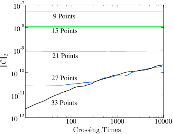
Figure 4: Constraints for 1-D Gaussian Linear Wave. Here we see the exponential convergence of the constraints with higher spatial resolution. At late times, the higher resolutions grow sublinearly in time, probably because of accumulated machine roundoff error.

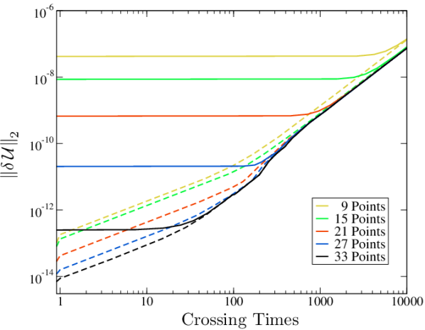
Figure 5: Error Energy for 1-D Gaussian Linear Wave. The solid lines show the error energy at 1/2 crossing times, with clearly visible exponential convergence at early times. The dashed lines show the error energy at integer crossing times for the same resolutions. The smallness of the error energy at early times demonstrates the low dispersion of the numerical method, as explained in the main text. At later times, the error is dominated by the quadratic growth explained in the text.

We find behavior comparable to the sinusoidal case, although as expected, more collocation points in the $x$-direction are needed to resolve the solution spatially (but we still use only a single point in each of the $y$- and $z$-dimensions). Note the exponential convergence of the constraints with increasing resolution in Fig. 4. The constraint growth in the highest resolution runs is slower than linear in time, and is probably caused by the accumulation of errors due to finite machine precision as discussed in Sec. IV.1.

Figure 5 presents the error energy for this run as the solid lines. At early times $||\delta\mathcal{U}||$ decreases with resolution exponentially to zero, as one would expect. At late times, however, $||\delta\mathcal{U}||$ converges toward a parabola. The amplitude of this parabola scales in proportion to $A^{2}$. In the rest of this section, we will first explain a subtlety arising when computing $||\delta\mathcal{U}||$, followed by a detailed explanation of why the terms $\mathcal{O}(A^{2})$ manifest themselves in parabolic behavior of $||\delta\mathcal{U}||$.

The comparison of the computed solution with the analytic solution is performed at the collocation points. By virtue of the transformation Eqs. (13) and (14), the errors are initially exactly zero at the collocation points. The spatial truncation error is nonzero of course, even at the initial time; it manifests itself by a deviation of the truncated series expansion from the analytic solution between collocation points. During the evolution, a linear wave will simply travel through the computational domain, returning to the original position after each light-crossing time. Since the spectral method has very small dispersion, the evolved shape remains the same. After each light-crossing time, therefore, the evolved solution again agrees to very high accuracy with the initial analytic solution at the collocation points. So, comparing the evolution with the analytic solution at integer multiples of the light-crossing time and at the collocation points will yield differences much smaller than spatial truncation error. Therefore, a fair comparison that includes the effects of spatial truncation error must not be performed at integer light-crossing times. These considerations are evident from Fig. 5, where the solid lines show the “true” $||\delta\mathcal{U}||$ observed with 1/2 light-crossing interval offset, which suffices because the number of collocation points is always odd. The artificially small error energy observed at every complete light-crossing interval is shown as dashed lines, confirming the excellent low-dispersion property of our method.

At late times the differences between observation at full and 1/2 crossing times are swamped by the parabolic growth in $||\delta\mathcal{U}||$. Similar parabolic deviations of the evolution from the solution of the linearized equations are observed for the other two linear wave evolutions, the 1-D and 2-D sinusoids (cf. Fig. 7). The growth in $\|\delta\,\mathcal{U}\|$ appears almost entirely due to growth in the $k=0$ mode of diagonal terms in $\delta g_{ij}$. Using evolutions of waves with different amplitudes and wavelengths, we have verified that this growth is proportional to $A^{2}t^{2}/\lambda^{2}$, where $A$ is the amplitude and $\lambda$ the wavelength of the disturbance. The constant of proportionality depends directly on the KST parameter $\gamma_{1}$ appearing in Eq. (4). This parameter controls the addition of a term $\gamma_{1}Ng_{ij}C$ to the ADM evolution equation for $K_{ij}$. The Hamiltonian constraint $C$ is roughly constant in time, and varies as $A^{2}/\lambda^{2}$. Since the $k=0$ mode of $\gamma_{1}Ng_{ij}C$ is roughly $\gamma_{1}\delta_{ij}C$, the $k=0$ mode of $K_{ii}$ will grow linearly with time in proportion to $\gamma_{1}A^{2}/\lambda^{2}$ for each $i$. That, in turn, will cause small quadratic growth in the $k=0$ mode of $g_{ii}$. For the more well-behaved cases (highest resolutions for the Gaussians; all cases for the sinusoids) this model is an excellent fit for the observed error energy.

IV.3 Two-Dimensional Linear Waves

The linear wave tests above may be modified by rotating the coordinates by $\pi/4$ about the $z$-axis, which gives a plane wave propagating along the $x$-$y$ diagonal. By increasing the size of the domain by a factor of $\sqrt{2}$ in each direction, the rotated solution can be made periodic while maintaining the same wavelength. This converts the spacetime from essentially one-dimensional to essentially two-dimensional. The purpose of this test is to ensure that the symmetry of the one-dimensional version does not hide sources of error (although propagation along a diagonal retains some symmetries). For these tests we use a single collocation point in the $z$-dimension, and we vary the (equal) number of collocation points in the $x$- and $y$-dimensions. We run these tests to $t=1000$—ten times longer than is recommended by the Apples with Apples collaboration—to better observe the stability properties. As shown in Fig. 6, the constraints for the sinusoidal wave increase with increasing $x$- and $y$-resolution (still using only a single point in the $z$-direction). The constraints for the Gaussian are very nearly the same as in the one-dimensional case. Again, the $A^{2}t^{2}/\lambda^{2}$ growth of $\|\delta\,\mathcal{U}\|$ is visible, as shown in Fig. 7.

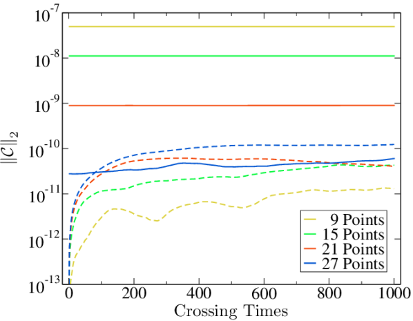
Figure 6: Constraints for 2-D Linear Waves. The solid lines represent the Gaussian wave, while the dashed lines represent the sinusoidal wave. The sinusoid is fully resolved spatially with 3 points. Going to higher resolutions merely introduces spatial errors in the unnecessary basis functions, which leads to an increase in the constraints with resolution.

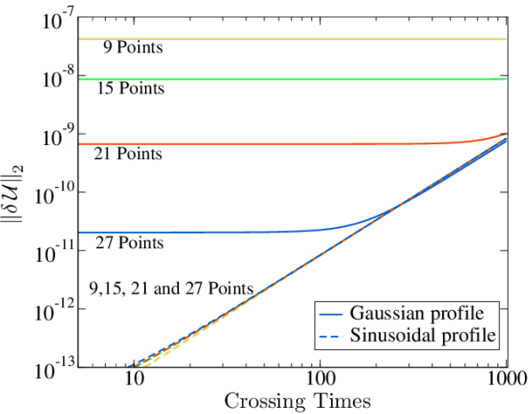
Figure 7: Error Energy for 2-D Linear Waves. The solid lines represent the Gaussian wave, while dashed lines represent the sinusoidal wave, both observed at 1/2 crossing times. As in the 1-D case (Fig. 5), both sets of evolutions converge to quadratic growth of the error caused by the Hamiltonian constraint, explained in the text.

V Gauge Wave

The next series of tests involves a simple but time-dependent gauge transformation of Minkowski space, in the form of a plane wave. The metric used for this Mexico City test has the form

$$ds^{2}=-(1+a)dt^{2}+(1+a)dx^{2}+dy^{2}+dz^{2}\ ,$$ (28)

$$a=A\sin\left[2\pi(x-t)\right]\ .$$ (29)

Two cases are considered: a low amplitude case $A=0.01$, and a high amplitude case $A=0.1$. This is the first test for which the nonlinear terms in the equations play an important role.

For the linear plane wave test in Section IV, we found that because we use a Fourier basis, we were able to fully resolve the sinusoidal waveform using only three collocation points. This is not true for the gauge-wave test, because in this case the extrinsic curvature (one of our evolved variables) is not a simple sinusoid. Instead, its only nonzero component is

$$K_{xx}=-\pi\,\frac{A\,\cos\left[2\pi(x-t)\right]}{\sqrt{1+A\,\sin\left[2\pi(x-t)\right]}}\ .$$ (30)

V.1 One-Dimensional Gauge Wave

We ran the one-dimensional test described above using a single collocation point in each of the $y$- and $z$-dimensions, and varying the resolution in the $x$-dimension. We find that for both $A=0.01$ and $A=0.1$ our evolution is stable and convergent. Our error energy and constraint violations show no signs of instability and are strictly better than the filtered two-dimensional evolutions discussed below. We omit plots for this test because the two-dimensional test is more challenging and more discriminating.

V.2 Two-Dimensional Gauge Wave

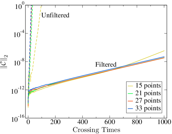
Figure 8: Constraints for High-Amplitude 2-D Gauge Wave. Dashed lines indicate the unfiltered behavior; solid lines indicate the filtered behavior. Note that, despite an effective loss of resolution, filtering greatly improves the stability of the evolution.

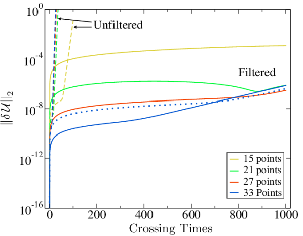
Figure 9: Error Energy for High-Amplitude 2-D Gauge Wave. As in Fig. 8, dashed lines are unfiltered, and solid lines are filtered. The growth of the filtered error energy is exponential in time. For the highest resolution the time step was cut in half ($dt=dx/80$) to reduce time-discretization error to the same level as spatial discretization error. The dotted line shows the same evolution with time step $dt=dx/40$, which is dominated by time discretization error.

A simple rotation of coordinates about the $z$-axis makes the wave described by Eqs. (28) and (29) propagate along the $x$-$y$ diagonal, as in the case of the linear wave. We use an equal number of collocation points in the $x$- and $y$-dimensions, and a single collocation point in $z$.

As for the one-dimensional gauge wave test, we run at two different amplitudes: $A=0.01$ and $A=0.1$. For low amplitude, $A=0.01$, our evolution of the 2-D gauge wave is stable and convergent. Again, we omit plots, as our results are strictly better than for the more interesting high-amplitude case.

For high amplitude, $A=0.1$, we find an exponentially growing nonconvergent numerical instability, as seen in the curves labeled “unfiltered” in Figs. 8 and 9. This instability does not appear for the low-amplitude case, nor does it appear for either amplitude in the one-dimensional gauge wave test.

The instability appears to be associated with aliasing caused by quadratic nonlinearities in the evolution equations; this is a well-known phenomenon that often occurs when applying spectral methods to nonlinear equations Boyd (1989). The basic mechanism for the instability can be understood by considering a truncated spectral expansion for some variable $u(x)$ in terms of $N$ basis functions $\phi_{k}(x)$:

$$u(x)=\sum_{k=0}^{N-1}u_{k}\phi_{k}(x)\ .$$ (31)

The correct spectral expansion of the expression $u(x)^{2}$ can be obtained by squaring Eq. (31); for most basis functions—including the Fourier series of Eq. (18)—this yields a sum over a total of $2N$, and not just $N$, basis functions. But we keep only $N$ basis functions (not $2N$) in our expansion, so the $k\geq N$ coefficients of the product must be eliminated. Ideally, these $k\geq N$ coefficients should be simply discarded and the $k<N$ coefficients should remain untouched. But it turns out that for the pseudospectral method of evaluating nonlinear terms (i.e., Fourier transform to obtain values at spatial collocation points, square these values, then Fourier transform back to spectral space), the power in the extra $k\geq N$ coefficients of the product does not disappear, but instead appears as excess power in some of the $k<N$ coefficients (“aliasing”). Repeating this process on each time step builds up this excess power and produces the instability.

Fortunately, there is a well-known remedy for instabilities caused by aliasing in nonlinear terms: suppose that the upper half (i.e., those with $k\geq N/2$) of the coefficients $u_{k}$ in Eq. (31) were all zero. Then the spectral expansion of $u(x)^{2}$ will have zeroes in all its $k\geq N$ coefficients, so there is no aliasing, and hence no instability. Therefore, we ensure that all coefficients with $k\geq k_{\mathrm{cut}}$ are zero by removing those coefficients from the initial data and from the right-hand side of the evolution equations. It turns out (see, for example, Chapter 11.5 of Ref. Boyd (1989)) that for a quadratic nonlinearity, it is sufficient to filter with $k_{\mathrm{cut}}=2N/3$ (and not $k_{\mathrm{cut}}=N/2$) to eliminate aliasing. As mentioned in Section II, the remaining number of nonzero coefficients must be odd, which is ensured by reducing $k_{\mathrm{cut}}$ by one if necessary.

The price we pay for stability via this filtering is that we must use a factor of $1.5$ more spectral coefficients (and collocation points) than without filtering in order to achieve the same level of spatial discretization error. Hence, we use more points for this test than for the previous ones: $N_{i}=15$, 21, 27, and 33 points. This leaves the effective resolutions at $\tilde{N}_{i}=9$, 13, 17, and 21 points, which are comparable to the resolutions we use in the unfiltered case. We see from Figs. 8 and 9 that filtering dramatically reduces the instability. The initial constraint violations in these runs, $\|\mathcal{C}\|\approx 10^{-12}$, are at the level of the finite machine precision, so increasing the resolution causes increased—not decreased—constraint violations.

V.3 Shifted Gauge Wave

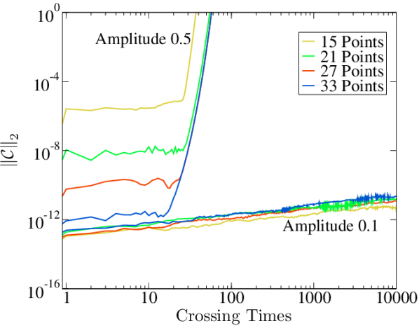
Figure 10: Constraints for Shifted Gauge Wave. Solid lines indicate $A=0.5$, and dashed lines indicate $A=0.1$. For both amplitudes we filter out the top $1/3$ spectral coefficients.

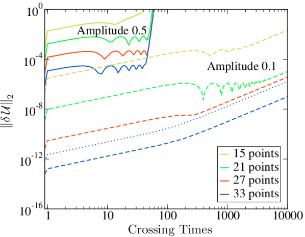
Figure 11: Error Energy for Shifted Gauge Wave. Solid lines indicate $A=0.5$, while dashed lines indicate $A=0.1$. The growth in the $A=0.1$ runs is roughly linear in time, accelerating to quadratic at later times. The dotted line indicates the standard time step ($dt=dx/40$) with $33$ points, which is dominated by temporal discretization error, while the blue dashed curve uses $dt=dx/80$.

We also show the results of a new “shifted gauge wave” test suggested for addition to the “Apples with Apples” suite Babiuc et al. (2006). For this test we evolve flat space with the usual Minkowski coordinates $(\hat{t},\hat{x},\hat{y},\hat{z})$ transformed to coordinates $(t,x,y,z)$ via

$$\hat{t} = t-\frac{A}{4\pi}\,\cos\left[2\pi(x-t)\right]\ ,$$ (32)

$$\hat{x} = x-\frac{A}{4\pi}\,\cos\left[2\pi(x-t)\right]\ ,$$ (33)

$$\hat{y} = y\ ,$$ (34)

$$\hat{z} = z\ .$$ (35)

This test includes the effects of a nonvanishing shift vector. We use the same computational domain and KST parameters as in the standard gauge wave tests above. The amplitude suggested in Ref. Babiuc et al. (2006) is $A=0.5$. We also run simulations with $A=0.1$.

At high amplitude, $A=0.5$, we see exponentially growing nonconvergent instabilities. Without filtering, the code crashes after just a few crossing times. By filtering out the top $1/3$ spectral coefficients as described above, the evolution can be extended as far as $t=60$. No other choice of filtering seems to improve this further. We also run the test with an amplitude of $A=0.1$. For this amplitude, the evolutions are stable with filtering but unstable without. Figs. 10 and 11 show the constraints and error energy for these evolutions. The initial constraint violations in these runs, $\|\mathcal{C}\|\approx 10^{-13}$, are at the level of the finite machine precision, so increasing the resolution causes increased, rather than decreased, constraint violations. The growth in $\|\delta\mathcal{U}\|$ seen in Fig. 11 is linear in time for $t<100$, becoming quadratic at late times. The quadratic in time growth is dominated by time-stepping error, which tests show is convergent. (Reducing this error to the level of spatial truncation error would require a prohibitive amount of computing time at the higher resolutions.)

VI Gowdy Spacetime

The Gowdy spacetimes are dynamic cosmological solutions that present a serious challenge to any numerical relativity code. The Gowdy spacetimes are vacuum cosmological models having two spatial Killing fields (planar symmetry) that expand from (or, when time-reversed, contract toward) a curvature singularity. Two particular examples of these spacetimes with relatively simple analytical forms were chosen for the Mexico City tests: one in which the spacetime expands away from the singularity; another in which it collapses toward the singularity.

VI.1 Expanding Form

The metric chosen for the expanding case is

$$ds^{2}=t^{-1/2}e^{\frac{\lambda-\lambda_{0}}{2}}(-dt^{2}+dz^{2})+t(e^{P}dx^{2}+e^{-P}dy^{2})\ ,$$ (36)

where

$$P(t,z)=J_{0}(2\pi t)\cos(2\pi z)\ ,$$ (37)

$$\lambda(t,z) = -2\pi tJ_{0}(2\pi t)J_{1}(2\pi t)\cos^{2}(2\pi z)$$ (38)

$$+2\pi^{2}t^{2}\left[J_{0}^{2}(2\pi t)+J_{1}^{2}(2\pi t)\right],$$

$\lambda_{0}=\lambda(1,1/8)$, and $J_{n}$ is a Bessel function. Asymptotically, $P$ approaches zero as time increases, and $\lambda$ increases linearly with time. Because the metric components are singular at $t=0$, the Mexico City test begins the evolution at $t=1$ and proceeds forward in time.

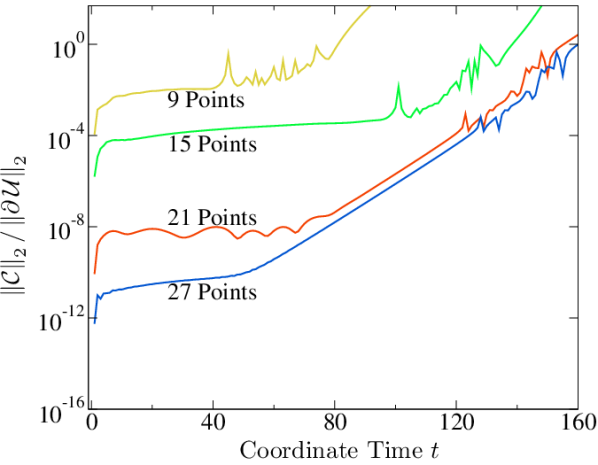
Figure 12: Constraints for Expanding Gowdy Spacetime. At early times, the exponential convergence of spectral methods is clearly visible. Soon, however, the evolutions are dominated by constraints growing roughly as $e^{t/5}$.

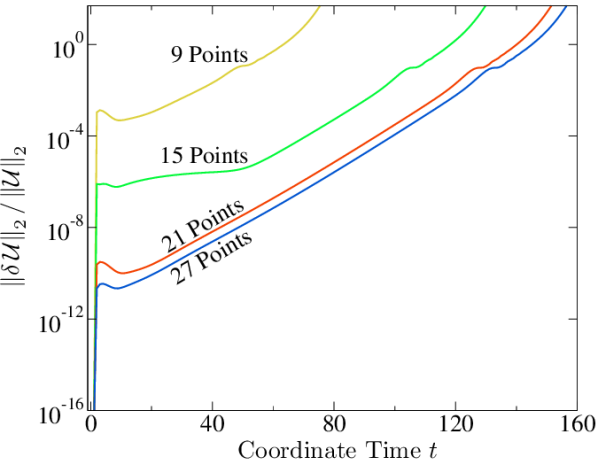
Figure 13: Error Energy for Expanding Gowdy Spacetime. The error energy converges with increased spatial resolution, but $\|\delta\mathcal{U}\|_{2}/\|\mathcal{U}\|_{2}$ grows like $e^{t/5}$.

The time step $\Delta t$ required for numerical stability is roughly given by the Courant condition $\Delta t\lesssim\Delta x/v$, where $\Delta x$ is the spacing between collocation points and $v$ is the coordinate speed of wave propagation, which in this case is the coordinate speed of light. For the Gowdy metric the coordinate speed of light in the $z$-direction is constant in time, but in the $x$- and $y$-directions it varies roughly like $t^{3/4}e^{t/2}$. Therefore, the maximum allowed time step decreases in time like $t^{-3/4}e^{-t/2}$, so for any fixed time step, the evolution will soon become numerically unstable if there is any perturbation in the $x$- or $y$-directions. This problem can be circumvented by running the simulation with just one point in the transverse directions, effectively eliminating any perturbation that could seed the instability.

Another difficulty with evolving the expanding Gowdy metric is that the metric components and derivatives become enormous very quickly. By $t\sim 725$ the numbers become larger than $10^{310}$, so the evolution cannot be easily handled using standard 64-bit floating-point arithmetic. Our evolutions do not actually crash until $t=700$; unfortunately errors dominate our evolutions long before this time, as seen in Fig. 13. The normalized error energy—along with the constraints shown in Fig. 12—grows roughly as $e^{t/5}$, and accuracy is completely lost in these evolutions by $t\sim 150$.

VI.2 Collapsing Form

The time coordinate in the Gowdy metric given above can be transformed so that the initial singularity is approached only asymptotically in the past. The new time coordinate, $\tau$, is defined by $\tau\equiv\frac{1}{c}\,\ln\left({t}/{k}\right)$, where $c=0.0021195119214607454$, and $k=9.6707698127640558$. The spacetime can be evolved backwards indefinitely without reaching the singularity; that is, the time step is chosen to be negative. For purposes of convenience, the evolution is begun at an initial time of $\tau=\tau(t_{0})$, where $t_{0}=9.8753205829098263$, which is a zero of $J_{0}(2\pi t)$.

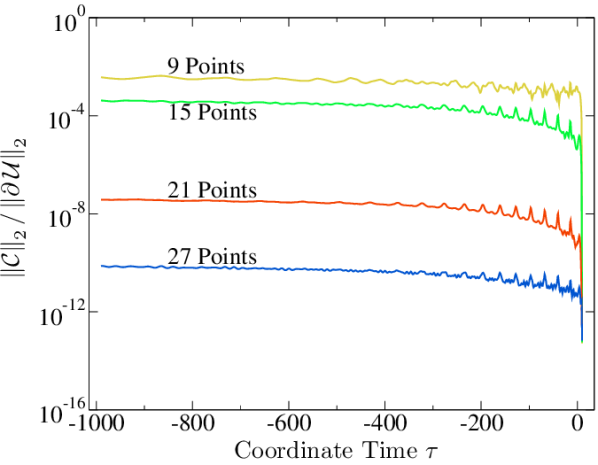
Figure 14: Constraints for Collapsing Gowdy Spacetime. Note that the simulation starts at $\tau\sim 9.875$, and proceeds backwards.

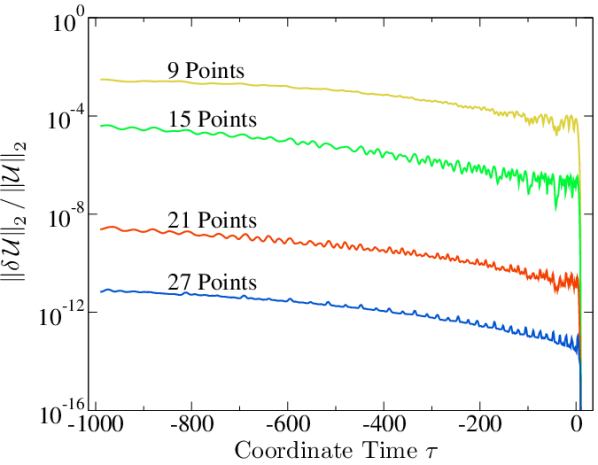
Figure 15: Error Energy for Collapsing Gowdy Spacetime. The simulation starts at $\tau\sim 9.875$, and proceeds backwards.

This evolution is far less challenging than the expanding case. This is because the lapse function is essentially an exponential in $\tau$, so that the spacetime is becoming less dynamical as the simulation progresses and $\tau$ becomes more negative. The main challenge in this test is resolving the spatial features of the solution. For spectral methods, the convergence should be exponential with increasing resolution, which is indeed the behavior shown in Figs. 14 and 15.

VII Discussion

We have applied the full suite of Mexico City tests Alcubierre et al. (2004)—modified suitably—to a pseudospectral implementation of the KST formulation of Einstein’s equations. We have also implemented the shifted gauge-wave test suggested by Babiuc, et al. Babiuc et al. (2006), and suggested a number of minor changes to the tests that make them better challenges for pseudospectral methods. These tests reveal that the KST equations with pseudospectral methods demonstrate excellent convergence and accuracy, along with very good stability in all but a few cases. We have derived a fundamental limit Eq. (25) for the time step accuracy possible in a method-of-lines numerical simulation, and have shown that our implementation is capable of quickly achieving that limit in the simple case of a sinusoidal linear wave. We have also shown that the use of filtering is very effective in reducing nonlinear aliasing instabilities.

The Mexico City tests provide a basic set of benchmarks for evaluating any numerical relativity code: allowing direct comparisons between different codes that use different numerical techniques and different formulations of the Einstein Equations. However, the tests in their present form make too many implicit assumptions about the evolution system and the numerical methods. Since the creation of the tests, numerical relativity codes have become more diverse: using a variety of improved numerical techniques (fixed and adaptive mesh refinement, higher order finite-differencing, multi-block methods, spectral methods) and at least two evolution systems (generalized harmonic and BSSN) capable of successfully evolving binary black hole spacetimes.

To accommodate the wide range of numerical methods and evolution systems now being used, future tests need to be formulated in more abstract terms. We recommend the following specific changes to the statement of the tests:

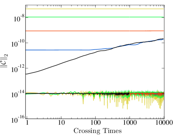
Figure 16: Comparing Constraints for 1-D Gaussian Linear Waves. Hamiltonian constraint norms (ragged curves) are much smaller than $\|\mathcal{C}\|$ for this test, so by themselves are not good diagnostics of constraint violations.

1. A code should demonstrate convergence, both spatial and temporal, appropriate for the numerical method used, for each of the tests (gauge wave, linear wave, Gowdy spacetime, etc.).

The number of grid points or the time step needed to achieve a given accuracy is highly dependent on the numerical implementation. Therefore, the test specifications should not dictate a certain number of grid points or a certain time-step size as the original formulation of the tests did.

1. The combined error of all evolution variables, and the combined constraint violation (including all constraints of an evolution system), cf. Eqs. (7) and (8), should be reported for each of the tests.

Prescriptions for examining errors of particular variables or constraints, such as those given in the original Mexico City tests, are not applicable to evolution systems that do not evolve those particular variables or constraints (e.g., tetrad or generalized harmonic evolution systems). In addition such prescriptions may not encompass all variables or constraints (as in the KST system), and may therefore fail to detect errors that accumulate only in a subset of the evolved variables. To illustrate this point, Fig. 16 shows both the total constraint energy $\|\mathcal{C}\|$, and the Hamiltonian constraint for the Gaussian linear wave (cf. Fig. 4). The Hamiltonian constraint turns out to be anomalously small for the KST system in this case, and so is not a good overall error indicator.

1. Use periodic Gaussian wave spatial profiles in the linear and gauge wave tests.

The sinusoidal spatial profiles specified in the original Mexico City tests with periodic boundary conditions provide an artificial advantage for spectral techniques. Periodic Gaussian profiles are no more difficult for finite difference codes, and provide a significantly greater challenge for spectral methods. Finally,

1. Output data at generic times, not at integer multiples of the light-crossing time.

Outputting data at exact integer multiples of the light-crossing time significantly underestimates the errors in codes with very small dissipation (such as spectral codes).

We believe these recommendations will make it easier to apply the Mexico City tests fairly to a far wider class of numerical relativity codes, and so facilitate apples-with-apples comparisons between these codes. We have learned a great deal about the subtle properties of our code by carefully running and analyzing these simple tests. We encourage other groups to make their results from these tests public so that meaningful and objective comparisons between codes can be made.