Interior of a Schwarzschild black hole revisited

Abstract

The Schwarzschild solution has played a fundamental conceptual role in general relativity, and beyond, for instance, regarding event horizons, spacetime singularities and aspects of quantum field theory in curved spacetimes. However, one still encounters the existence of misconceptions and a certain ambiguity inherent in the Schwarzschild solution in the literature. By taking into account the point of view of an observer in the interior of the event horizon, one verifies that new conceptual difficulties arise. In this work, besides providing a very brief pedagogical review, we further analyze the interior Schwarzschild black hole solution. Firstly, by deducing the interior metric by considering time-dependent metric coefficients, the interior region is analyzed without the prejudices inherited from the exterior geometry. We also pay close attention to several respective cosmological interpretations, and briefly address some of the difficulties associated to spacetime singularities. Secondly, we deduce the conserved quantities of null and timelike geodesics, and discuss several particular cases in some detail. Thirdly, we examine the Eddington-Finkelstein and Kruskal coordinates directly from the interior solution. In concluding, it is important to emphasize that the interior structure of realistic black holes has not been satisfactorily determined, and is still open to considerable debate.

I Introduction

The Schwarzschild solution has proved to play a fundamental importance in conceptual discussions of general relativity, and beyond, for instance, regarding event horizons, spacetime singularities and aspects of quantum field theory in curved spacetimes. It has also been important providing the first insights regarding the phenomenon of gravitational collapse OppSnyd and inspired the construction of theoretical models of relativistic stars relativistic-stars . Before the mid-1960s, the object now known as a black hole, was referred to as a collapsed star Thorne-etal or as a frozen star Novikov , and it was only in 1965 that marked an era of intensive research into black hole physics. Relatively to the issue of experimental tests of the Schwarzschild solution, the exterior geometry has been extremely successful in explaining, for instance, the precession of Mercury’s perihelion, and the phenomenon of the bending of light, where the exterior Schwarzschild gravitational field acts as a gravitational lens.

Despite of its important role, one still encounters, in the literature, the existence of misconceptions and a certain ambiguity inherent in the Schwarzschild solution. For instance, a problematic aspect is the presence of an event horizon, which in the Schwarzschild black hole solution acts as a one-way membrane, permitting future-directed null or timelike curves to cross only from the exterior to the interior region. It acts as a boundary of all events which, in principle, may be observed by an exterior observer. It is believed that the gravitational collapse of a compact body results in a singularity hidden beyond an event horizon. If the singularity were visible to the exterior region, one would have a naked singularity, which would open the realm for wild speculation. This led to Penrose’s cosmic censorship conjecture Penrose , which stipulates that all physically reasonable spacetimes are globally hyperbolic, forbidding the existence of naked singularities, and only allowing singularities to be hidden behind event horizons. The cosmic censorship conjecture has been an active area of research and the source of considerable controversy. For the interior black hole solution, a remarkable change occurs in the nature of spacetime, namely, the external spatial radial and temporal coordinates exchange their character to temporal and spatial coordinates, respectively. Thus, the interior solution represents a non-static spacetime, as the metric coefficients are now time-dependent. This also implies that a singularity occurs at a spacelike hypersurface, $t=0$. Thus, no observer, interior or exterior to the Schwarzschild radius, will be able to observe the formation, or for that matter, the physical effects of the singularity Narlikar . These aspects show the existence of inconsistencies and a certain ambiguity inherent in the Schwarzschild solution.

Still relatively to the issue of the black hole event horizon, a widespread misconception in the literature is that a test particle approaches the Schwarzschild radius at the speed of light for all observers, and not as a limiting process for a static observer located at the event horizon given by the null hypersurface $r\rightarrow 2M$, where $M$ is the black hole mass. We shall use geometrized units, i.e., $G=c=1$, for notational convenience, throughout this paper. If one accepts that a particle has the speed of light with respect to a static observer, at $r=2M$, then using the local special relativity velocity composition law, the observer concludes that the particle has the speed of light with respect to all observers, which is another way of saying that in the frame of a photon all particles have speed $v=1$. Of course, the frame of the photon is not a physical frame. Indeed, it should be emphasized that an observer cannot remain at rest at $r=2M$, as it implies an infinite acceleration to do so. Another erroneous extrapolation of $v\rightarrow 1$ at $r=2M$, is that timelike particles attain velocities superior to the speed of light in the black hole region $0<r<2M$, and thus justifying the existence of tachyons, or for that matter of particles with velocities superior to the speed of light in the framework of general relativity Gold-Sabb . All things considered, it should be stressed once again that one can only use static observers in the spacetime region characterized by $r>2M$. And it was shown that the test particle does indeed cross the event horizon with a velocity less than the speed of light Janis with respect to an appropriate physical observer. An exact general expression was further deduced, in terms of the constants of motion of both a test particle and an observer moving along radially infalling geodesics CrawTereno , given by

$$v^{2}\big{|}_{r=2M}=1-\frac{4E_{1}^{2}E_{2}^{2}}{\left(E_{1}^{2}+E_{2}^{2}\right)^{2}}\,$$ (1)

where $E_{1}$ and $E_{2}$ are the constants of motion for the test particle and the observer, respectively. This expression shows that the value of the velocity at $r=2M$ is indeed less than $1$, unless $E_{1}$ or $E_{2}$ are zero or infinite (see Ref. CrawTereno for details, and Ref. Bolos for further discussions).

Relatively to spacetime singularities, a key aspect is whether they are a disaster for the theory, as they imply the breakdown of predictability. Various definitions of singularities can be encountered in the literature, ranging from specific invariants, constructed from the curvature tensor and its covariant derivatives, becoming infinite, to the notion of geodesic incompleteness. Accordingly, one encounters several attitudes to spacetime singularities Earman : Firstly, singularities are mere artifacts of unrealistic and idealized models where infinities occur. Secondly, general relativity entails singularities, according to the Penrose-Hawking theorems in the context of geodesic incompleteness, and fails to accurately describe nature. Thirdly, one may have a more optimistic viewpoint, as expressed by Misner, who views the existence of singularities, “not as proof of our ignorance, but as a source from which we can derive much valuable understanding of cosmology”Misner .

Much of the scepticism related to the concepts of event horizons and spacetime singularities, outlined above, and others such as the information paradox, has inspired new and fascinating ideas Mazur ; gravastars ; Dymnikova ; darkstars , namely by replacing the interior solution, and thus, doing away with the problems related to these issues. In this context, it is interesting to note the emergence of a new picture for an alternative final state of gravitational collapse, where an interior compact object is matched to an exterior Schwarzschild vacuum spacetime, at or near where the event horizon is expected to form. These alternative models do not possess a singularity at the origin and have no event horizon, as its rigid surface is located at a radius slightly greater than the Schwarzschild radius. In particular, the gravastar (gravitational vacuum star) picture, proposed by Mazur and Mottola Mazur , has an effective phase transition at/near where the event horizon is expected to form, and the interior is replaced by a de Sitter condensate. It has also been argued that there is no way of distinguishing a Schwarzschild black hole from a gravastar from observational data AKL . However, a realistic model for the gravitational collapse leading to compact interior objects is still lacking. We also emphasize that, although interesting in themselves, the solutions that do away with the interior singularity and the event horizon Mazur ; gravastars ; Dymnikova ; darkstars sweep the inherent conceptual difficulties of black holes under the rug, and that the interior structure of realistic black holes has not been satisfactorily determined, being still open to considerable debate.

In this work, we shall review and analyze the interior Schwarzschild solution in some detail. In the literature, the interior geometry is considered as a continuity of the exterior geometry. Therefore, for instance, infalling test particles are considered ending up at a central singularity located at $r=0$. However, the latter singularity is a spacelike hypersurface, and the test particles are not directed towards a privileged point, but directed along a temporal direction, in order to not violate causality. Thus, if one looks at the interior geometry as a continuation of the exterior static solution, one comes across some extremely interesting conceptual difficulties, that question the very concept of a black hole. In this work we shall address some of these difficulties. We shall start by obtaining the metric for the interior region without inferring directly to the traditional Schwarzschild solution. With this geometry at hand, one may analyze this interior region, without the prejudices inherited from the exterior region. However, we emphasize that we shall compare both regions where it is convenient to do so. We find new interesting features and peculiarities not encountered in the literature, and show that this scenario can be interpreted as a cosmological solution.

This paper is outlined in the following manner: Firstly, in Section II, we deduce the interior metric by considering time-dependent metric fields, paying close attention to several cosmological interpretations of this solution. We also address some of the difficulties associated to spacetimes singularities, and argue that it is perhaps possible for an observer to know if he is inside or outside the Schwarzschild radius, by examining an invariant of a covariant derivative of the curvature tensor. Secondly, in Sections III and IV, we deduce the conserved quantities of null and timelike geodesics in some detail, discussing several particular cases. Thirdly, in Sections V and VI, we analyze the Eddington-Finkelstein and Kruskal coordinates directly from the interior solution. Finally, we conclude in Section VII.

II Interior spacetime

II.1 Spacetime metric

We shall be interested in the spacetime metric given by

$$ds^{2}=-B(z,t)\,dt^{2}+A(z,t)dz^{2}+F(z,t)\,d\Omega^{2}\,,$$ (2)

where $d\Omega^{2}=d\theta^{2}+\sin^{2}{\theta}\,d\phi^{2}$ and $(t,z,\theta,\phi)$ are the spacetime coordinates. Assume that $F(z,t)=F(t)$, so that the line element with $t={\rm const}$ and $z={\rm const}$ describes a $2-$sphere with an area given by $A=4\pi F(t)$. In particular, we shall consider the specific case of $F(t)=t^{2}$.

To set the nomenclature, note that the mathematical analysis and the physical interpretation will be simplified using a set of orthonormal basis vectors. These may be interpreted as the proper reference frame of a set of observers who remain at rest in the coordinate system $(t,z,\theta,\phi)$, with $(z,\theta,\phi)$ fixed. Denote the basis vectors in the coordinate system as ${\bf e}_{t}$, ${\bf e}_{z}$, ${\bf e}_{\theta}$, and ${\bf e}_{\phi}$. Then, using the following transformation, ${\bf e}_{\hat{\alpha}}=\Lambda^{\beta}_{\;\hat{\alpha}}\;{\bf e}_{\beta}$, with

$$(\Lambda^{\beta}_{\;\hat{\alpha}})=\left[\begin{array}[]{cccc}B^{-1/2}&0&0&0\\ 0&A^{-1/2}&0&0\\ 0&0&t^{-1}&0\\ 0&0&0&(t\sin\theta)^{-1}\end{array}\right]\,,$$ (3)

one finds

$$\left\{\begin{array}[]{l}{\bf e}_{\hat{t}}=B^{-1/2}\;{\bf e}_{t}\\ {\bf e}_{\hat{z}}=A^{-1/2}\;{\bf e}_{z}\\ {\bf e}_{\hat{\theta}}=t^{-1}\;{\bf e}_{\theta}\\ {\bf e}_{\hat{\phi}}=(t\sin\theta)^{-1}\;{\bf e}_{\phi}\,.\end{array}\right.$$ (8)

In this basis the metric components assume their Minkowskian form, $g_{\hat{\alpha}\hat{\beta}}=\eta_{\hat{\alpha}\hat{\beta}}={\rm diag}(-1,1,1,1)$.

The Einstein field equation, in an orthonormal reference frame, is given by

$$G_{\hat{\mu}\hat{\nu}}=8\pi\,T_{\hat{\mu}\hat{\nu}},$$ (9)

where $T_{\hat{\mu}\hat{\nu}}$ is the stress-energy tensor and $G_{\hat{\mu}\hat{\nu}}$ is the Einstein tensor, given by $G_{\hat{\mu}\hat{\nu}}=R_{\hat{\mu}\hat{\nu}}-\frac{1}{2}g_{\hat{\mu}\hat{\nu}}R$. $R_{\hat{\mu}\hat{\nu}}$ is the Ricci tensor, which is defined as a contraction of the Riemann (or curvature) tensor, $R_{\hat{\mu}\hat{\nu}}=R^{\hat{\alpha}}_{\;\;\hat{\mu}\hat{\alpha}\hat{\nu}}$, and $R$ is the scalar curvature defined as a contraction of the Ricci tensor, $R=R^{\hat{\alpha}}{}_{\hat{\alpha}}$.

The Einstein tensor, given in the orthonormal reference frame, $G_{\hat{\mu}\hat{\nu}}$, yields for the metric (2) the following non-zero components

$$G_{\hat{t}\hat{t}} = \frac{\dot{A}}{ABt}+\frac{1}{t^{2}}+\frac{1}{Bt^{2}}\,,$$ (10)

$$G_{\hat{z}\hat{z}} = \frac{\dot{B}}{tB^{2}}-\frac{1}{t^{2}}-\frac{1}{Bt^{2}}\,,$$ (11)

$$G_{\hat{z}\hat{t}} = \frac{B^{\prime}}{tB\sqrt{AB}}\,,$$ (12)

$$G_{\hat{\theta}\hat{\theta}} = -\frac{1}{2AB}\Bigg{[}\frac{\dot{A}}{t}-\frac{A\dot{B}}{Bt}+\ddot{A}-B^{\prime\prime}$$ (13)

$$-\frac{\dot{A}^{2}}{2A}+\frac{A^{\prime}B^{\prime}}{2A}+\frac{(B^{\prime})^{2}}{2B}-\frac{\dot{A}\dot{B}}{2B}\Bigg{]}\,,$$

$$G_{\hat{\phi}\hat{\phi}} = G_{\hat{\theta}\hat{\theta}}\,,$$ (14)

where a prime denotes a derivative with respect to the coordinate $z$, and the overdot a derivative with respect to the temporal coordinate, $t$.

We shall consider a vacuum solution, i.e. $G_{\hat{\mu}\hat{\nu}}=0$. From the addition of Eqs. (10) and (11), we verify

$$G_{\hat{t}\hat{t}}+G_{\hat{z}\hat{z}}=\frac{1}{tB}\left(\frac{\dot{B}}{B}+\frac{\dot{A}}{A}\right)=0\,,$$ (15)

so that the solution $AB=C$, with $C=C(z)$ is obtained. It is possible to absorb the function $C(z)$, defining a new spatial coordinate $\bar{z}=\sqrt{C}\,z$, so that without a significant loss of generality one may set $C=1$. One may conclude from this analysis that $A=1/B$.

From Eq. (12),

$$G_{\hat{z}\hat{t}}=\frac{B^{\prime}}{tB\sqrt{AB}}=0\,,$$ (16)

we verify $B^{\prime}=0$, so that $B=B(t)$, implying $A=A(t)$. Note that $B=B(t)$ is related to the proper time $d\tau^{2}=B(t)\,dt^{2}$, so that one may impose that $B(t)>0$.

Now, substituting the relationship $A=1/B$ into Eq. (10), one finally deduces that

$$A(t)=B^{-1}(t)=\frac{C_{1}}{t}-1\,,$$ (17)

where $C_{1}$ is a constant of integration with time dimension. From the condition $B(t)>0$, and consequently $A(t)>0$, this solution is only valid for $t<C_{1}$.

Defining the constant of integration as $C_{1}=2\xi$ the metric (2) finally takes the form

$$ds^{2} = -\left(\frac{2\xi}{t}-1\right)^{-1}\,dt^{2}+\left(\frac{2\xi}{t}-1\right)dz^{2}$$ (18)

$$+t^{2}\,(d\theta^{2}+\sin^{2}{\theta}\,d\phi^{2})\,.$$

The constant $\xi$ may be determined from a direct confrontation with the exterior Schwarzschild solution, and is given by $\xi=M$, where $M$ is the black hole mass. It may take the physical significance of a characteristic time for the existence of universes in the interior Schwarzschild solution, as may be inferred from the cosmological interpretation of the interior metric, given by Eq. 2, which we consider in the next subsection.

II.2 Cosmological interpretation

This interior solution illustrates a particularly strange, yet physically meaningful picture of the universe within the event horizon. Thus, we shall consider some interesting astrophysical and cosmological interpretations of this solution. A quick glance at the metric (18) is enough to convince one that this also corresponds to an anisotropic and homogeneous cosmological solution. In fact, considering the Kantowski-Sachs KS solution given by

$$ds^{2}=-d\bar{t}^{\,2}+A^{2}(\bar{t}\,)\,dz^{2}+C^{2}(\bar{t}\,)\,(d\theta^{2}+\sin^{2}{\theta}\,d\phi^{2})\,,$$ (19)

where $A(\bar{t}\,)$ and $C(\bar{t}\,)$ are the scale factors of the geometry, one verifies that both metrics are identical, by taking into account the following transformation

$$d\bar{t}^{\,2}=\left(\frac{2\xi}{t}-1\right)^{-1}\,dt^{2}\,.$$ (20)

An alternative approach would be to consider a time-dependent parameter $\xi=\xi(t)$ Vollick , so that one could generalize metric (18) to

$$ds^{2} = -\left[\frac{2\xi(t)}{t}-1\right]^{-1}\,dt^{2}+\left[\frac{2\xi(t)}{t}-1\right]dz^{2}$$ (21)

$$+t^{2}\,(d\theta^{2}+\sin^{2}{\theta}\,d\phi^{2})\,.$$

The Einstein tensor given in an orthonormal reference frame has the following non-zero components

$$G_{\hat{t}\hat{t}} = \frac{2\dot{\xi}}{t^{2}}\,,$$ (22)

$$G_{\hat{z}\hat{z}} = -\frac{2\dot{\xi}}{t^{2}}\,,$$ (23)

$$G_{\hat{\theta}\hat{\theta}} = G_{\hat{\phi}\hat{\phi}}=-\frac{\ddot{\xi}}{t}\,,$$ (24)

where the overdot denotes a derivative with respect to the time coordinate $t$, as before. Note that this solution implies $\rho=-p_{z}$, where $\rho$ and $p_{z}$ are the energy density and the pressure along the $z-$direction, much in the spirit of Refs. gravastars ; Dymnikova . Note that the geometry (21) where $\xi$ is time-dependent is not a solution of the vacuum Einstein equations. In addition, even though $\rho=-p_{z}$, they are time-dependent, i.e., the corresponding “cosmological constant” is not constant at all.

The above-mentioned case provides some very interesting cosmological solutions, in rather different contexts, however, they shall be presented elsewhere Doran . Several cosmological scenarios have also been proposed, in which a universe emerges from the interior of a black hole (see, for instance, Ref. Easson and references therein). In the present work, we shall only consider several interesting interpretations of universes within the Schwarzschild radius, relatively to the metric (18).

Consider the interior solution as measured by an observer at rest relatively to the space coordinates, i.e., $dz=d\theta=d\phi=0$. In this case, from the metric (18), we have

$$d\tau=\pm\frac{dt}{\sqrt{2\xi/t-1}}\,.$$ (25)

For the positive sign, we have the solution

$$\tau=-\sqrt{t(2\xi-t)}+\xi\arctan\left[\frac{t-\xi}{\sqrt{t(2\xi-t)}}\right]+\frac{\pi\xi}{2}\,,$$ (26)

where the constant of integration has been chosen to provide $\tau=0$ for $t=0$. Note that as $t=2\xi$, we have $\tau=\xi\pi$, so that as coordinate time increases, the proper time as measured by observers at rest also increase.

The evolution of this universe may be further explored Brehme by considering the negative sign of Eq. (25), which yields the following solution

$$\tau=\sqrt{t(2\xi-t)}-\xi\arctan\left[\frac{t-\xi}{\sqrt{t(2\xi-t)}}\right]+\frac{3\pi\xi}{2}\,.$$ (27)

The constant of integration has been chosen to provide $\tau=\xi\pi$ for $t=2\xi$. For this case the coordinate time decreases from $t=2\xi$ to $t=0$, however, proper time increases from $\tau=\pi\xi$ to $\tau=2\pi\xi$. This behavior is represented in Fig. 1.

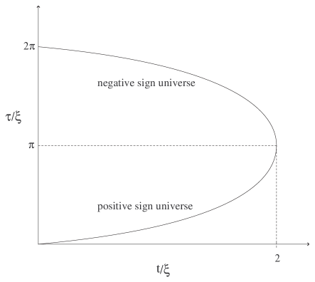
Figure 1: Plot of the proper time for observers at rest relatively to the $(z,\phi,\theta)$ coordinate system. The evolution of a universe begins at $t=0$, and proper time $\tau=0$. As coordinate time flows from $t=0$ to $t=2\xi$, proper time runs from $\tau=0$ to $\tau=\pi\xi$. This corresponds to the positive sign solution of Eq. (26). Now, allowing for the time coordinate to flow backwards from $t=2\xi$ to $t=0$, proper time as measured by observers at rest, inexorably runs forward from $\tau=\pi\xi$ to $\tau=2\pi\xi$. This corresponds to the negative sign solution of Eq. (27). See the text for details.

Taking into account the metric (18), we verify that it possesses rotational invariance, as the spatial surfaces corresponding to $z={\rm const}$, represent a $2-$sphere with an area given by $A=4\pi t^{2}$. The proper distance between two simultaneous events along a determined spatial direction, for instance $d\phi=0$ and $\theta=\pi/2$, is given by

$$D_{p}=\int_{z_{1}}^{z_{2}}\sqrt{\frac{2\xi}{t}-1}\;dz=\sqrt{\frac{2\xi}{t}-1}\;\Delta z\,.$$ (28)

Note that a singularity occurs for $t=0$, as can also be verified from the curvature tensor. The proper distance between two particles at rest separated by a constant $\Delta z$, decreases along the $z-$direction as coordinate time flows from $t=0$ to $t=2\xi$, and increases as coordinate time flows backwards from $t=2\xi$ to $t=0$. Despite the fact that one may not talk about an asymptotic limit, for the interior solution, it is interesting to note that the spacetime assumes an instantaneous Minkowski form, for $t=\xi$, although the curvature does not become zero.

The proper distance between two simultaneous events along a spatial trajectory with $dz=0$ and $\theta=\pi/2$, is given by

$$D_{p}=\int_{\phi_{1}}^{\phi_{2}}t\,d\phi=t\;\Delta\phi\,,$$ (29)

which increases as $t$ varies from $t=0$ to $t=2\xi$, and decreases when the temporal coordinate runs backwards from $t=2\xi$ to $t=0$.

Therefore, one may conclude by assuming the evolution of a universe beginning at $t=0$, where a singularity occurs along the $z-$direction, however, with no extension along the angular direction, $\phi$. As coordinate time flows from $t=0$ to $t=2\xi$, observers at rest move together, i.e., their proper distance decreases to zero, and move apart along the angular coordinate attaining a maximum at $t=2\xi$. Now, allowing for the coordinate to flow backwards from $t=2\xi$ to $t=0$, proper time as measured by observers, at rest relatively to the $(z,\phi,\theta)$ coordinate system, inexorably runs forward from $\tau=\pi\xi$ to $\tau=2\pi\xi$. For this case, observers move apart along the $z-$direction and collapse along the angular coordinate.

In this example, the difference of choosing an interior observer, without the prejudices inherited from the exterior geometry, is striking. While for the exterior observer, infalling particles tend to a central singularity, from the interior point of view, the proper distance along the $z-$direction increases, showing the existence of a cigar-like singularity. We emphasize that the latter occurs along a spacelike hypersurface. Another difference worth mentioning is that the exterior observer considers a spherically symmetric geometry, while the interior observer may consider the geometry plane, as points for different $\phi$ are parallel to one another (see Ref. Brehme for details regarding this issue).

II.3 Singularities

The Schwarzschild solution has played a fundamental role in conceptual discussions of general relativity, in particular, regarding spacetime singularities, as mentioned in the Introduction. A key aspect of singularities in general relativity is whether they are a disaster for the theory, as it implies the breakdown of predictability. Attitudes in the literature range from Earman : singularities are mere artifacts of unrealistic and idealized models; general relativity entails singularities, but fails to accurately describe nature; and one may view the existence of singularities “not as proof of our ignorance, but as a source from which we can derive much valuable understanding of cosmology”, quoting Misner in the latter attitude Misner .

A way of detecting singularities is to find where the energy density or the spacetime curvature become infinite and the usual description of the spacetime breaks down. However, to be sure that there is an essential singularity which cannot be transformed away by a coordinate transformation, invariants are constructed from the curvature tensor, such as $R$, $R_{\mu\nu}R^{\mu\nu}$, $R^{\mu\nu\alpha\beta}R_{\mu\nu\alpha\beta}$, and from certain covariant derivatives of the curvature tensor. For instance, in the Schwarzschild spacetime there is an essential curvature singularity at $r=0$ in the sense that along any non-spacelike trajectory falling into the singularity, as $r\rightarrow 0$, the so-called Kretschman scalar tends to infinity, i.e., $K=R^{\mu\nu\alpha\beta}R_{\mu\nu\alpha\beta}\rightarrow\infty$, as shall be shown below. In this case, however, all future directed non-spacelike geodesics which enter the event horizon at $r=2M$ must fall into this curvature singularity within a finite value of the affine parameter. So, all such curves are future geodesically incomplete. For the black hole region, given by the metric (18), the scalar Kretschmann polynomial, $K$, is given by

$$R^{\mu\nu\alpha\beta}R_{\mu\nu\alpha\beta}=\frac{48\xi^{2}}{t^{6}}\,,$$ (30)

showing that a curvature singularity occurs at $t=0$.

It is remarkable that a change of sign occurs in the following scalar KLA , as an observer traverses the event horizon

$$R^{\mu\nu\alpha\beta;\gamma}R_{\mu\nu\alpha\beta;\gamma}=-720\frac{(2\xi-t)\xi^{2}}{t^{9}}\,.$$ (31)

Note that the invariant is zero on the horizon $t=2\xi$. It is perhaps possible that this invariant is devoid of a fundamental significance. However, it is generally known that using the curvature tensor and some of its covariant derivatives, the analysis gives a complete description of the geometry, and are directly measurable. Since these quantities are coordinate invariant, the problems associated with a specific choice of the coordinate system vanish. This argument may be used in favor of separating the interior from the exterior region.

II.4 Tidal forces

The tidal acceleration felt by an observer at rest is given by

$$\Delta a^{\hat{\mu}}=-R^{\hat{\mu}}_{\;\;\hat{\nu}\hat{\alpha}\hat{\beta}}\,U^{\hat{\nu}}\eta^{\hat{\alpha}}U^{\hat{\beta}}\,,$$ (32)

where $U^{\hat{\mu}}=\delta^{\hat{\mu}}_{\;\;\hat{0}}$ is the observer’s four velocity and $\eta^{\hat{\alpha}}$ is the separation between two arbitrary parts of his body. Note that $\eta^{\hat{\alpha}}$ is purely spatial in the observer’s reference frame, as $U^{\hat{\mu}}\eta_{\hat{\mu}}=0$, implying $\eta^{\hat{t}}=0$. $R^{\hat{\mu}}_{\;\;\hat{\nu}\hat{\alpha}\hat{\beta}}$ is the Riemann tensor, given in the orthonormal reference frame, and has the following non-zero components

$$R_{\hat{z}\hat{\theta}\hat{z}\hat{\theta}} = R_{\hat{z}\hat{\phi}\hat{z}\hat{\phi}}=-\frac{\xi}{t^{3}}\,,$$ (33)

$$R_{\hat{z}\hat{t}\hat{z}\hat{t}} = -R_{\hat{\theta}\hat{\phi}\hat{\theta}\hat{\phi}}=-\frac{2\xi}{t^{3}}\,,$$ (34)

$$R_{\hat{\theta}\hat{t}\hat{\theta}\hat{t}} = R_{\hat{\phi}\hat{t}\hat{\phi}\hat{t}}=\frac{\xi}{t^{3}}\,.$$ (35)

Taking into account the antisymmetric nature of $R^{\hat{\mu}}_{\;\;\hat{\nu}\hat{\alpha}\hat{\beta}}$ in its first two indices, we verify that $\Delta a^{\hat{\mu}}$ is purely spatial with the components

$$\Delta a^{\hat{i}}=-R^{\hat{i}}{}_{\hat{t}\hat{j}\hat{t}}\,\eta^{\hat{j}}=-R_{\hat{i}\hat{t}\hat{j}\hat{t}}\,\eta^{\hat{j}}.$$ (36)

Finally, using the components of the Riemann tensor, the tidal acceleration has the following components

$$\Delta a^{\hat{z}} = \frac{2\xi}{t^{3}}\,\eta^{\hat{z}}\,,$$ (37)

$$\Delta a^{\hat{\theta}} = -\frac{\xi}{t^{3}}\,\eta^{\hat{\theta}}\,,$$ (38)

$$\Delta a^{\hat{\phi}} = -\frac{\xi}{t^{3}}\,\eta^{\hat{\phi}}\,.$$ (39)

Note a stretching along the $z-$direction, and a contraction along the orthogonal directions. These stretchings and contractions are now time-dependent, contrary to their counterparts in the exterior region, and as $t\rightarrow 0$, the tidal forces diverge.

III Conserved quantities

Consider the Euler-Lagrange equations

$$\frac{d}{d\lambda}\left(\frac{\partial L}{\partial\dot{x}^{\mu}}\right)-\frac{\partial L}{\partial x^{\mu}}=0\,,$$ (40)

where the overdot here represents a derivative with respect to the affine parameter defined along the geodesic, which has the physical interpretation of a proper time for timelike geodesics. Consider the following Lagrangian

$$L(x^{\mu},\dot{x}^{\mu})=\frac{1}{2}g_{\mu\nu}\dot{x}^{\mu}\dot{x}^{\nu}\,.$$ (41)

If the metric tensor does not depend on a determined coordinate, $x^{\mu}$, one obtains an extremely important result. For this case, Eq. (40) reduces to

$$\frac{d}{d\lambda}\left(\frac{\partial L}{\partial\dot{x}^{\mu}}\right)=0\,.$$ (42)

This implies that the quantity given by

$$p_{\mu}=\frac{\partial L}{\partial\dot{x}^{\mu}}=g_{\mu\nu}\,\dot{x}^{\nu}\,,$$ (43)

is constant along any geodesic. Using the Lagrangian nomenclature, one denotes $x^{\mu}$ a cyclic coordinate, and $p_{\mu}$ the respective conjugate momentum. The existence of cyclic coordinates allows one to obtain integrals of the geodesic equation, and provides certain quantities that are conserved along the movement of the particle.

Applying the above analysis to the line element (18), one verifies that the metric tensor is independent of the coordinates $z$ and $\phi$, so that the conserved quantities are given by

$$P_{\phi} = g_{\phi\phi}\,\dot{\phi}=t^{2}\dot{\phi}=Q\,,$$ (44)

$$P_{z} = g_{zz}\,\dot{z}=\left(\frac{2\xi}{t}-1\right)\dot{z}\,.$$ (45)

$Q$ may be interpreted as the angular momentum per unit mass, and $P_{z}$ possesses the dimensions of a velocity. As $P_{z}$ may take any real value, we shall consider it as a mere conserved quantity, without any physical significance.

The line element (18) may be rewritten in terms of the constants defined above, for the particular case of $\theta=\pi/2$, in the following manner

$$\dot{t}^{2}=P_{z}^{2}+\left(\frac{Q^{2}}{t^{2}}-k\right)\,\left(\frac{2\xi}{t}-1\right)\,,$$ (46)

where $k=0$ is defined for null geodesics, and $k=-1$ for timelike geodesics.

For timelike geodesics, $k=-1$, the conserved quantities $P_{z}$ and $Q$ may also be determined from the initial conditions. For this purpose it will prove useful to provide an intrinsic definition of velocity, which we shall include next for self-completeness.

Consider the four-velocity, $U^{\mu}$, tangent to the worldline of an observer, and a four-dimensional spacetime, $\Sigma$, orthogonal to $U^{\mu}$. Define the operator

$$h^{\mu}{}_{\nu}=g^{\mu}{}_{\nu}+U^{\mu}U_{\nu}\,,$$ (47)

which has the property of projecting any four-vector on the tangent space of the hypersurface, $\Sigma$, so that $h^{\mu}{}_{\nu}\,U^{\nu}=0$. Thus, one may express the metric tensor in the following form

$$ds^{2} = g_{\mu\nu}\,dx^{\mu}\,dx^{\nu}$$ (48)

$$= -\left(U_{\mu}\,dx^{\mu}\right)^{2}+h_{\mu\nu}\,dx^{\mu}\,dx^{\nu}$$

$$= -d\tau_{*}^{2}+dl^{2}\,.$$

The quantity $d\tau_{*}=-U_{\mu}\,dx^{\mu}$ is the projection of the displacement of a particle, $dx^{\mu}$, along the velocity of the observer, so that the particle has a displacement of $dl^{2}=h_{\mu\nu}\,dx^{\mu}\,dx^{\nu}$, along $\Sigma$. Thus, the velocity may then be defined as

$$V^{2}=\left(\frac{dl}{d\tau_{*}}\right)^{2}=\frac{h_{\mu\nu}\,dx^{\mu}\,dx^{\nu}}{\left(U_{\mu}\,dx^{\mu}\right)^{2}}\,.$$ (49)

Now, consider that the observer is at rest in the $x^{\mu}$ coordinates, so that his/her four-velocity is given by $U^{\mu}=(U^{t},0,0,0)$, with $U^{t}=(-g_{tt})^{-1/2}$. Thus, we have

$$h_{\mu\nu}=g_{\mu\nu}-\frac{g_{\mu t}g_{\nu t}}{g_{tt}}\,,$$ (50)

and

$$d\tau_{*}^{2}=-\frac{\left(g_{\mu t}\,dt\right)^{2}}{g_{tt}}\,,$$ (51)

so that Eq. (49) may be finally written as

$$V^{2}=\frac{\left(g_{\mu t}g_{\nu t}-g_{tt}g_{\mu\nu}\right)\,dx^{\mu}\,dx^{\nu}}{\left(g_{\mu t}\,dx^{\mu}\,\right)^{2}}\,.$$ (52)

This result is identical to the one obtained by Landau and Lifschitz Landau .

Now, using the metric (18) and considering $\theta=\pi/2$, Eq. (52) takes the form

$$V^{2}=-\frac{g_{zz}}{g_{tt}}\left(\frac{dz}{dt}\right)^{2}-\frac{g_{\phi\phi}}{g_{tt}}\left(\frac{d\phi}{dt}\right)^{2}\,.$$ (53)

and finally using Eq. (46), we have

$$P_{z}^{2}=g_{zz}\left(\frac{V^{2}}{1-V^{2}}-\frac{Q^{2}}{t^{2}}\right)\,.$$ (54)

Considering the particular case of $d\theta=d\phi=0$, i.e., fo a test particle that moves along the $z-$direction Eq. (54) takes the form

$$P_{z}^{2}=\left(\frac{2\xi}{t}-1\right)\left(\frac{V^{2}}{1-V^{2}}\right)\,.$$ (55)

The qualitative behavior for the positive values of $P_{z}$, in the parameter space of $t$ and $V$, is represented in Fig. 2. Note that $P_{z}$ may take arbitrarily large values as $V\rightarrow 1$ or as $t\rightarrow 0$.

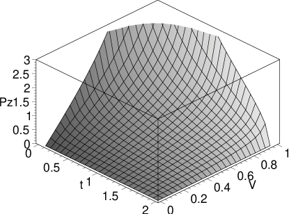
Figure 2: Qualitative behavior of the positive values of $P_{z}$ in the parameter space $t$ and $V$, where we have considered $\xi=1$. See the text for details.

For a point particle with an initial velocity $V_{0}<1$ and initial time $t=T$, then $P_{z}$ is given by $P_{z}^{2}=(2\xi/T-1)V_{0}^{2}/(1-V_{0}^{2})$. Note that if the test particle is at rest, $V_{0}=0$, at an instant $T\neq 2\xi$, then it will always remain at rest as $P_{z}=0$. If the particle came in from the exterior region, it possesses a conserved quantity $E$ along its geodesic. Despite the fact that after the crossing of the event horizon its character changes into a constant with the dimensions of a velocity, its numerical value is conserved, i.e., $E=P_{z}$. The constant may assume different positive values depending on its initial conditions. However, as reflected by Eq. (45), $P_{z}$ may assume negative values as well, so that one may conclude that geodesic particles moving along a decreasing $z$ coordinate, and increasing $t$ coordinate, (or for that matter, an increasing $z$ coordinate and decreasing $t$, taking into account the cosmological interpretation of Section II.2) cannot have come in from the exterior region.

Equation (54) may be rewritten as

$$Q^{2}=t^{2}\left(\frac{V^{2}}{1-V^{2}}-\frac{P_{z}^{2}}{g_{zz}}\right)\,.$$ (56)

If $\theta=\pi/2$ and $dz=0$, then the constant reduces to

$$Q^{2}=t^{2}\left(\frac{V^{2}}{1-V^{2}}\right)\,.$$ (57)

For a point particle with an initial velocity $V_{0}<1$ and initial time $t=T$, then $Q^{2}=T^{2}V_{0}^{2}/(1-V_{0}^{2})$. If the particle is initially at rest then $Q=0$.

IV Geodesics

An advantage of analyzing the interior region, not as a continuation of the exterior region, but as a manifold on its own, is a verification of the great difference existing between the geodesics of both regions. If one treats the interior solution as a cosmological solution, one may verify which type of universe one is dealing with, or which geodesics are analogous with those existing in our universe.

Consider the geodesic equation given by

$$\frac{d^{2}x^{\mu}}{d\lambda^{2}}+\Gamma^{\mu}{}_{\alpha\beta}\,\frac{dx^{\alpha}}{d\lambda}\frac{dx^{\beta}}{d\lambda}=0\,,$$ (58)

where $\lambda$ is an affine parameter defined along the geodesic. It is a simple matter of exercising some index gymnastics to verify the equivalence of the geodesic equation and the Euler-Lagrange equations (40).

Now, the geodesic equation, Eq. (58), for the metric (18) may be written in the following form

$$\ddot{t}-\frac{\xi(2\xi/t-1)}{t^{2}}\,\dot{z}^{2}+\frac{m}{t^{2}(2\xi/t-1)}\,\dot{t}^{2}+t(2\xi/t-1)\,\dot{\theta}^{2}$$

$$\hskip 71.13188pt+t\,\sin^{2}\theta\,(2\xi/t-1)\,\dot{\phi}^{2}=0\,,$$ (59)

$$\ddot{z}-\frac{2\xi}{t^{2}(2\xi/t-1)}\,\dot{z}\,\dot{t}=0\,,$$ (60)

$$\ddot{\theta}+\frac{2}{t}\,\dot{t}\,\dot{\theta}-\sin\theta\,\cos\theta\,\dot{\phi}^{2}=0\,,$$ (61)

$$\ddot{\phi}+\frac{2}{t}\,\dot{t}\,\dot{\phi}-2\cot\theta\,\,\dot{\theta}\,\dot{\phi}=0\,.$$ (62)

Considering the particular case of $\theta=\pi/2$, and using the conserved quantities, the three primary integrals are given by

$$\dot{z}=\frac{P_{z}}{2\xi/t-1}\,,$$ (63)

$$\dot{\phi}=\frac{Q}{t^{2}}\,,$$ (64)

$$\frac{\dot{t}^{2}}{2\xi/t-1}-\left(\frac{2\xi}{t}-1\right)\,\dot{z}^{2}-t^{2}\,\dot{\phi}^{2}=k\,,$$ (65)

which are identical to Eqs. (44)-(46). (See Ref. Kiselev for an interesting analysis of radial geodesics confined under the Schwarzschild horizon.) We shall next analyze null and timelike geodesics in some detail, and finally summarize the main results in Tables 1 and 2, respectively.

IV.1 Null geodesics

Equation (46), for null geodesics, reduces to

$$P_{z}^{2}=\dot{t}^{2}-\left(\frac{Q^{2}}{t^{2}}\right)\,\left(\frac{2\xi}{t}-1\right)\,.$$ (66)

Consider null geodesics along the $z-$direction, i.e., with $d\theta=d\phi=0$, so that we simply have

$$P_{z}=\frac{dt}{d\lambda}\,,$$ (67)

where $\lambda$ is an affine parameter defined along the geodesic.

For this case, the line element reduces to

$$ds^{2}=-\left(\frac{2\xi}{t}-1\right)^{-1}\,dt^{2}+\left(\frac{2\xi}{t}-1\right)\,dz^{2}\,.$$ (68)

Considering null geodesics, $ds^{2}=0$, i.e, $dt=\pm(2\xi/t-1)dz$, we have as solution

$$z=\mp\left[t+2\xi\ln\left(1-\frac{t}{2\xi}\right)\right]+C\,,$$ (69)

where $C$ is a constant of integration. Equation (69) is represented in Fig. 3.

Figure 3: Plot of null geodesics, along the $z-$direction, i.e., with $d\theta=d\phi=0$. See the text for details.

Note that traditionally the solution with $dt<0$ corresponds to a black hole solution, either with an increasing or decreasing $z$ coordinate, i.e., $dz>0$ or $dz<0$, respectively. A white hole solution corresponds to $dt>0$, either with $dz>0$ or $dz<0$. We also emphasize the importance of analyzing the interior solution separately, as in the literature the radial coordinate $r$ (considered in the Schwarzschild exterior) is generally considered as a coordinate that measures distances, in the interior. It is usually treated as a temporal coordinate to note that $r$ decreases (increases) for an observer in a black hole (white hole).

It is also of interest to study the case of $\theta=\pi/2$ and $dz=0$. Note that these are not circular orbits, as the $z$ coordinate can no longer be considered as a radial coordinate. Equation (45) provides $P_{z}=0$, and thus Eq. (66) may be rewritten as

$$\dot{t}^{2}=\left(\frac{Q^{2}}{t^{2}}\right)\left(\frac{2\xi}{t}-1\right)\,.$$ (70)

The line element, for this particular case takes the form

$$ds^{2}=-\left(\frac{2\xi}{t}-1\right)^{-1}\,dt^{2}+t^{2}\,d\phi^{2}\,.$$ (71)

The null geodesic, $ds^{2}=0$, provides $d\phi/dt=\pm 1/\sqrt{t(2\xi-t)}$, which has the following solution

$$\phi=\arcsin\left(\frac{t}{\xi}-1\right)+\frac{\pi}{2}\,,$$ (72)

or $t=\xi[1+\sin(\phi-\pi/2)]$. One may also obtain the equivalent solution, given by

$$\phi(t)=\arctan\left(\frac{t-\xi}{\sqrt{t(2\xi-t)}}\right)+\frac{\pi}{2}\,.$$ (73)

The constant of integration has been chosen to provide $\phi=0$ for $t=0$. Note that for $t=2\xi$, then $\phi=\pi$. For this case one verifies that a photon only traverses half-way around this particular universe.

	$\dot{t}=\sqrt{P_{z}^{2}+\left(Q^{2}/t^{2}\right)\,\left(2\xi/t-1\right)}$
	$\dot{z}=\left(2\xi/t-1\right)^{-1}\,P_{z}$
	$\dot{\phi}=Q/t^{2}$
$dz=0$	$\dot{t}=\sqrt{\left(Q^{2}/t^{2}\right)\,\left(2\xi/t-1\right)}$
	$\dot{\phi}=Q/t^{2}$
$d\phi=0$	$\dot{t}=P_{z}$
	$\dot{z}=\left(2\xi/t-1\right)^{-1}\,P_{z}$

Table 1: Summary of the equations of motion for null geodesics, considering the particular case of $\phi=\pi/2$. See the text for details.

IV.2 Timelike geodesics

Equation (46), for timelike geodesics, takes the form

$$P_{z}^{2}=\dot{t}^{2}-\left(\frac{Q^{2}}{t^{2}}+1\right)\,\left(\frac{2\xi}{t}-1\right)\,.$$ (74)

From the conserved quantities one may determine various expressions relating the time coordinate and the proper time. For instance, Eq. (74) may be expressed in the following form

$$d\tau=\pm\left[P_{z}^{2}+\left(\frac{Q^{2}}{t^{2}}+1\right)\left(\frac{2\xi}{t}-1\right)\right]^{-1/2}\;dt\,.$$ (75)

Substituting Eq. (54) in the above expression provides

$$d\tau^{2}=(1-V^{2})\left(\frac{2\xi}{t}-1\right)^{-1}\;dt^{2}\,.$$ (76)

This is an expression valid for a generic trajectory, and one readily verifies that the variation of proper time does not depend explicitly on the constants $P_{z}$ and $Q$.

One may also deduce, from Eq. (45), a relationship between the variation of proper time and the spatial coordinate, namely, $\Delta\tau=(g_{zz}/P_{z})\Delta z$. Consider the specific case of $P_{z}=1$, so that $\Delta\tau=g_{zz}\Delta z$, and fixing $\Delta z$, note that variations in proper time tend to infinity as $t\rightarrow 0$. This is another interesting example, as viewed from the interior, in that the test particle does not attain the singularity in his proper time.

Taking into account the specific case of $\theta=\pi/2$ and $d\phi=0$, which implies $Q=0$, along the direction of the $z$ coordinate, we have

$$P_{z}^{2}=\left(\frac{dt}{d\tau}\right)^{2}-\left(\frac{2\xi}{t}-1\right)\,,$$ (77)

from which we deduce

$$\frac{d\tau}{dt} = \pm\left[\left(\frac{2\xi}{t}-1\right)+P_{z}^{2}\right]^{-1/2}\,.$$ (78)

Taking into account the specific case of $P_{z}^{2}>1$, Eq. (78) may be integrated to provide the following proper time

$$\tau(t) = \pm(P_{z}^{2}-1)^{-3/2}\Big{\{}-\sqrt{t(2\xi-t+P_{z}^{2}t)(P_{z}^{2}-1)}+$$ (79)

$$+\xi\ln\left[\frac{\xi+t(P_{z}^{2}-1)}{\sqrt{P_{z}^{2}-1}}+\sqrt{t(2\xi-t+P_{z}^{2}t)}\right]\Bigg{\}}+C\,,$$

where $C$ is a constant of integration. If $P_{z}^{2}=1$, then the proper time is given by

$$\tau(t) = \mp\sqrt{\frac{2t}{\xi}}\;\frac{t}{3}+C\,.$$ (80)

For the particular case of $P_{z}^{2}<1$, Eq. (78) provides the following solution

$$\tau(t) = \pm(1-P_{z}^{2})^{-3/2}\Big{\{}-\sqrt{t(2\xi-t+P_{z}^{2}t)(1-P_{z}^{2})}+$$ (81)

$$+\xi\arctan\left[\frac{(1-P_{z}^{2})t-\xi}{\sqrt{t(2\xi-t+P_{z}^{2}t)(1-P_{z}^{2})}}\right]\Bigg{\}}+C\,.$$

Recall that the constant of motion may also be determined from the initial conditions, so that substituting Eq. (55), with the initial conditions $v_{0}$ and $T$, into Eq. (78), we finally have

$$d\tau=\left[\left(\frac{2\xi}{T}-1\right)\left(\frac{v_{0}^{2}}{1-v_{0}^{2}}\right)+\left(\frac{2\xi}{t}-1\right)\right]^{-1/2}\;dt\,.$$ (82)

The line element for $d\theta=d\phi=0$ is given by

$$ds^{2}=-\left(\frac{2\xi}{t}-1\right)^{-1}\,dt^{2}+\left(\frac{2\xi}{t}-1\right)\,dz^{2}\,,$$ (83)

which, taking into account Eqs. (45) and (77), takes the following form

$$\left(\frac{dt}{dz}\right)^{2}=\left(\frac{2\xi}{t}-1\right)^{2}\left[1+\left(\frac{2\xi}{t}-1\right)/P_{z}^{2}\right]\,.$$ (84)

In particular, for $P_{z}=1$, the above equation may be integrated to yield the solution

$$z=\mp\frac{2(6\xi+t)}{3}\sqrt{\frac{t}{2\xi}}\pm 4\xi\;{\rm arctanh}\left(\sqrt{\frac{t}{2\xi}}\right)\,,$$ (85)

It may be shown that this solution is qualitatively analogous to the plots of Fig. 3.

One of the most surprising results is that the trajectories of particles at rest are geodesics, contrary to the exterior where particles at rest are necessarily accelerated. As $P_{z}$ is a conserved quantity, a particle at rest, $z={\rm const}$, will always remain at rest. Despite the fact of the presence of strong gravitational fields in the interior of a black hole, test geodesic particles at rest relatively to the coordinate system may exist, which is due to the non-static character of the interior geometry. For an alternative approach, consider $dz=d\theta=d\phi=0$. In this case, from $d\tau=\pm(2\xi/t-1)^{-1/2}\,dt$, we have the following solution

$$\tau=\pm\sqrt{t(2\xi-t)}\mp\xi\arctan\left[\frac{t-\xi}{\sqrt{t(2\xi-t)}}\right]+C\,.$$ (86)

This solution was briefly considered in subsection II.2. The constant may be chosen by considering that for $t=0$ we have $\tau=0$. For the maximum coordinate time variation, $\Delta t=2\xi$, the corresponding proper time variation is $\Delta\tau=\xi\pi$. This is precisely the lifetime for the of existence of geodesic particles inside the black hole (white hole), i.e., these test particles exist for a finite proper time, $\xi\pi$. One verifies that Eq. (86) differs radically from its exterior counter-part. In the exterior region the proper time interval is inferior to the coordinate time interval, and is interpreted as the time interval of an observer located sufficiently far from the event horizon. A fundamental issue is that in the exterior region, the time coordinate is physically meaningful, as it corresponds to the proper time measured by observers at an asymptotically large value of the radial coordinate, $r$. In the interior region $d\tau=dt$ is but a mere instantaneous coincidence.

For the particular case of timelike geodesic particles at rest relatively to the $z$ coordinate, with $dz=0$ and $\theta=\pi/2$, we have $P_{z}^{2}=0$. As emphasized above, the trajectory around the $z-$axis cannot be interpreted as a circular orbit. The proper time for this trajectory is determined from the following expression

$$d\tau^{2}=\left[\left(\frac{Q^{2}}{t^{2}}+1\right)\left(\frac{2\xi}{t}-1\right)\right]^{-1}\,dt^{2}\,.$$ (87)

The velocity of a particle along this timelike geodesic, i.e., $dz=0$ and $\theta=\pi/2$, as measured by an observer at rest, taking into account Eq. (52), is given by

$$V^{2}=-\frac{g_{\phi\phi}}{g_{tt}}\left(\frac{d\phi}{dt}\right)^{2}=\left(\frac{2\xi}{t}-1\right)\,\frac{Q^{2}}{t^{2}\dot{t}^{2}}=\frac{Q^{2}}{t^{2}+Q^{2}}\,.$$ (88)

This expression may also be obtained from Eq. (57). Note that as $t\rightarrow 0$, then $V\rightarrow 1$. At $t=2\xi$, we verify that the particle attains a finite minimum value, given by $V^{2}=Q^{2}/(Q^{2}+4\xi^{2})$.

For the particular case of $dz=d\phi=0$ and $\theta=\pi/2$, we verify that the constants of motion are zero, $P_{z}=Q=0$, implying that the timelike geodesic particles remain at rest. An important conclusion is inferred from the conserved quantities for particles at rest. As is well known, an incoming geodesic particle from the exterior, has a conserved quantity $E$, which is interpreted as the energy per unit mass, along its trajectory. However, this constant of motion in the interior of the event horizon changes its physical significance, but its numerical value remains invariant. If $P_{z}=0$ is verified, this is equivalent to state that the test particle entered from the exterior with $E=0$. Now, the energy per unit mass is defined as $E=(1-2M/r)/(1-v_{0}^{2})$, so that $E=0$ corresponds to $r=2M$. This means that the particle started off from the horizon, which is a null surface. Thus, for the particular case of $P_{z}=0$, one may conclude that a geodesic timelike particle at rest in the interior of the horizon cannot have come in from the exterior region.

	$\dot{t}=\sqrt{P_{z}^{2}+\left(Q^{2}/t^{2}+1\right)\,\left(2\xi/t-1\right)}$
	$\dot{z}=\left(2\xi/t-1\right)^{-1}\,P_{z}$
	$\dot{\phi}=Q/t^{2}$
$dz=0$	$\dot{t}=\sqrt{\left(Q^{2}/t^{2}+1\right)\,\left(2\xi/t-1\right)}$
	$\dot{\phi}=Q/t^{2}$
$d\phi=0$	$\dot{t}=\sqrt{P_{z}^{2}+\left(2\xi/t-1\right)}$
	$\dot{z}=\left(2\xi/t-1\right)^{-1}\,P_{z}$
$dz=0$	$\dot{t}=\sqrt{\left(2\xi/t-1\right)}$
$d\phi=0$

Table 2: Summary of the equations of motion for timelike geodesics, considering the particular case of $\phi=\pi/2$. See the text for details.

V Eddington-Finkelstein coordinates

The Eddington-Finkelstein transformation is traditionally considered a transformation that permits the analysis of trajectories from $0<r<\infty$. However, in a general manner, the inversion of the character of the coordinates is not manifest. Therefore, to manifest this difference, we shall treat the Eddington-Finkelstein transformations directly from the interior metric (18).

For null geodesics along the $z-$direction, Eq. (69) provides the following solutions

$$z_{\mp}=\mp\left[t+2\xi\ln\left(1-\frac{t}{2\xi}\right)\right]+C\,.$$ (89)

The solution with the negative sign shows that $z$ increases as $dt<0$, and decreases as $dt>0$; from the solution with the positive sign, one may infer that $z$ increases as $dt>0$, and decreases as $dt<0$.

Consider now the following transformations

$$z^{\prime} = z_{-}+2\xi\ln\left(1-\frac{t}{2\xi}\right)\quad\Rightarrow\quad z^{\prime}=-t+C\,,$$ (90)

$$z^{\prime\prime} = z_{+}-2\xi\ln\left(1-\frac{t}{2\xi}\right)\quad\Rightarrow\quad z^{\prime\prime}=t+C\,.$$ (91)

In the exterior region of the event horizon, solutions for $dt<0$ are excluded, as one admits that the temporal coordinate increases. In the interior region two distinct cases need to be separated, namely, for $dt<0$, which traditionally is denoted a black hole, and $dt>0$, a white hole.

Taking into account the definition $z^{\prime}$, one may rewrite the metric (18) as

$$ds^{2}=\left(\frac{2\xi}{t}-1\right)\,dz^{\prime 2}+\frac{4\xi}{t}\,dz^{\prime}dt+\left(\frac{2\xi}{t}+1\right)\,dt^{2}+t^{2}\,d\Omega^{2}\,,$$ (92)

which is no longer singular at $t=2\xi$.

Now metric (92) may be simplified by introducing a null coordinate, denoted the advanced time parameter in analogy with the exterior solution

$$v^{\prime}=z^{\prime}+t=z_{-}+2\xi\,\ln\left(1-\frac{t}{2\xi}\right)+t\,,$$ (93)

so that the metric (18) takes the form

$$ds^{2}=\left(\frac{2\xi}{t}-1\right)\,dv^{\prime 2}+2\,dtdv^{\prime}+t^{2}\,d\Omega^{2}\,.$$ (94)

This is the line element of Eddington-Finkelstein for the advanced time parameter, which is regular at the instant $t=2\xi$.

Analyzing the specific case of $ds^{2}=d\theta=d\phi=0$, the metric (94) provides the following solutions

$$dv^{\prime}=0,\qquad{\rm or}\qquad\left(\frac{2\xi}{t}-1\right)dv^{\prime}=-2\,dt\,.$$ (95)

Recalling that $dv^{\prime}=dz^{\prime}+dt$, the above cases with

$$dz^{\prime} = -dt\,,$$ (96)

$$\frac{dt}{dz^{\prime}} = -\frac{2\xi-t}{2\xi+t}\,,$$ (97)

have the following solutions

$$z^{\prime} = -t+C\,,$$ (98)

$$z^{\prime} = t+4\xi\ln\left(1-\frac{t}{2\xi}\right)+C\,.$$ (99)

These are plotted in Fig. 4, for different values of the constant $C$. Note that both solutions obey $dz^{\prime}/dt<0$. A black hole solution corresponds to $dt<0$, and consequently $dz^{\prime}>0$; and analogously, a white hole solution corresponds to $dt>0$ and $dz^{\prime}<0$.

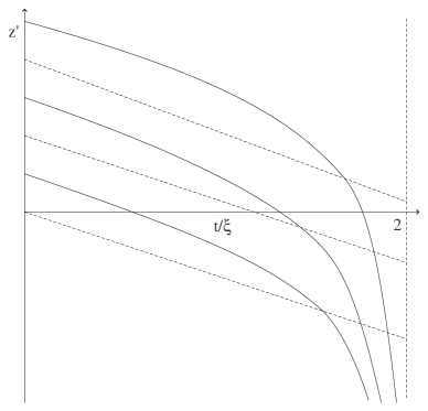
Figure 4: Eddington-Finkelstein diagram for the advanced temporal parameter. A black hole solution corresponds to $dt<0$, and consequently $dz^{\prime}>0$; and analogously, a white hole solution corresponds to $dt>0$ and $dz^{\prime}<0$.

Applying an analogous procedure for the retarded temporal parameter, $w^{\prime\prime}$, constructed from $z^{\prime\prime}$,

$$w^{\prime}=z^{\prime\prime}-t\Rightarrow w^{\prime}=z_{+}-2\xi\,\ln\left(1-\frac{t}{2\xi}\right)-t\,,$$ (100)

and consequently

$$ds^{2}=\left(\frac{2\xi}{t}-1\right)\,dw^{\prime 2}-2\,dtdw^{\prime}+t^{2}\,d\Omega^{2}\,.$$ (101)

As is manifest from the line elements (94) and (101), the metric coefficients are regular at $t=2\xi$.

For the case $ds^{2}=d\theta=d\phi=0$, the metric (101) provides the following relationships

$$dz^{\prime\prime} = dt\,,$$ (102)

$$\frac{dt}{dz^{\prime\prime}} = \frac{2\xi-t}{2\xi+t}\,,$$ (103)

with the respective solutions

$$z^{\prime\prime} = t+C\,,$$ (104)

$$z^{\prime\prime} = -t-4\xi\ln\left(1-\frac{t}{2\xi}\right)\,.$$ (105)

These are plotted in Fig. 5, for different values of the constant $C$. Both solutions obey $dz^{\prime\prime}/dt>0$, with $dt<0$ and $dz^{\prime\prime}<0$ corresponding to a black hole solution; and $dt>0$ and $dz^{\prime\prime}>0$ to a white hole solution, respectively.

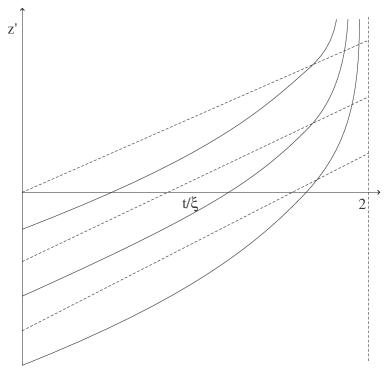
Figure 5: Eddington-Finkelstein diagram for the retarded temporal parameter. A black hole solution corresponds to $dt<0$, and consequently $dz^{\prime}<0$; and analogously, a white hole solution corresponds to $dt>0$ and $dz^{\prime}>0$.

VI Kruskal coordinates

Consider the difference obtained from Eqs. (93) and (100), given by

$$v^{\prime}-w^{\prime}=4\xi\ln\left(1-\frac{t}{2\xi}\right)+2t\,,$$ (106)

from which one may obtain the following equalities

$$1-\frac{t}{2\xi} = \exp\left(\frac{v^{\prime}-w^{\prime}}{4\xi}\right)\exp\left(-\frac{t}{2\xi}\right)\,,$$ (107)

$$dt = -(dv^{\prime}-dw^{\prime})\frac{2\xi-t}{2t}\,.$$ (108)

Substituting these expressions in Eq. (94), one obtains

$$ds^{2}=\left(\frac{2\xi}{t}-1\right)dw^{\prime}dv^{\prime}+t^{2}(d\theta^{2}+\sin^{2}\theta\,d\phi^{2})\,.$$ (109)

Now, introducing the Kruskal coordinates for the region $t<2\xi$ ($r<2M$), i.e.,

$$w^{\prime\prime} = \exp\left(-\frac{w^{\prime}}{4\xi}\right)\,,$$ (110)

$$v^{\prime\prime} = \exp\left(\frac{v^{\prime}}{4\xi}\right)\,.$$ (111)

Substituting these expressions in Eq. (107), we finally have

$$w^{\prime\prime}v^{\prime\prime}=\left(1-\frac{t}{2\xi}\right)\exp\left(\frac{t}{2\xi}\right)\,.$$ (112)

Equations (110)-(111) may be rewritten as

$$dw^{\prime} = -\frac{dw^{\prime\prime}}{w^{\prime\prime}}\,4\xi\,,$$ (113)

$$dv^{\prime} = \frac{dv^{\prime\prime}}{v^{\prime\prime}}\,4\xi\,,$$ (114)

which substituting into metric (109), we have the following

$$ds^{2}=-\frac{32\xi^{3}}{t}\exp\left(-\frac{t}{2\xi}\right)\;dw^{\prime\prime}dv^{\prime\prime}+t^{2}(d\theta^{2}+\sin^{2}\theta\,d\phi^{2})\,.$$ (115)

It is still possible to introduce the following transformations

$$t_{*} = \frac{1}{2}(v^{\prime\prime}+w^{\prime\prime})\,,$$ (116)

$$r_{*} = \frac{1}{2}(v^{\prime\prime}-w^{\prime\prime})\,,$$ (117)

so that we have $dt_{*}^{2}-dr_{*}^{2}=dv^{\prime\prime}\,dw^{\prime\prime}$. The line element finally assumes the form

$$ds^{2}=\frac{32\xi^{3}}{t}\exp\left(-\frac{t}{2\xi}\right)\;\left(-dt_{*}^{2}+dr_{*}^{2}\right)+t^{2}\,d\Omega^{2}\,.$$ (118)

The new coordinates may be rewritten as

$$t_{*} = \frac{1}{2}\left[\exp\left(\frac{v^{\prime}}{4\xi}\right)+\exp\left(-\frac{w^{\prime}}{4\xi}\right)\right]$$ (119)

$$= \left(1-\frac{t}{2\xi}\right)^{1/2}\exp\left(\frac{t}{4\xi}\right)\,\cosh\left(\frac{z}{4\xi}\right)$$

$$r_{*} = \frac{1}{2}\left[\exp\left(\frac{v^{\prime}}{4\xi}\right)-\exp\left(-\frac{w^{\prime}}{4\xi}\right)\right]$$ (120)

$$= \left(1-\frac{t}{2\xi}\right)^{1/2}\exp\left(\frac{t}{4\xi}\right)\,\sinh\left(\frac{z}{4\xi}\right)\,.$$

These expressions may be written

$$t_{*}^{2}-r_{*}^{2}=\left(1-\frac{t}{2\xi}\right)\,\exp\left(\frac{t}{2\xi}\right)\,,$$ (121)

which is the equation for a hyperbole, and may also be expressed as

$$\frac{r_{*}}{t_{*}}=\tanh\left(\frac{z}{4\xi}\right)\,,$$ (122)

which represent straight lines with $z={\rm const}$. See Fig. 6.

The singularity at $t=0$, written in terms of the new coordinates, is given by

$$t_{*}=\pm\sqrt{r_{*}^{2}+1}\,.$$ (123)

For $r_{*}=0$, we have $t_{*}=1$. For $t=2\xi$, we have $t_{*}=\pm r_{*}$, i.e., $\tanh(z/4\xi)=\pm 1$, which implies $z\rightarrow\pm\infty$. These relationships may be visualized in Fig. 6. We have also added the exterior region, for comparison purposes (see, for instance, Ref. Wald ).

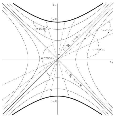
Figure 6: Kruskal diagram for the interior region of the Schwarzschild spacetime. We have added some details in the exterior region for comparison. See the text for details.

With this analysis at hand, one may consider the following motion of a timelike test particle, as viewed from an interior observer. The test particle starts its movement at the event $E_{1}$, arriving at the surface of $t=2\xi$ and $z=-\infty$, at event $E_{2}$. After an excursion in the exterior region, the test particle re-enters into the interior region at event $E_{3}$, corresponding to $t=2\xi$ and $z=+\infty$, and finally ends up in the spacelike singularity at $t=0$, at event $E_{4}$. Note an extremely curious feature of this movement, as viewed from an interior observer. The test particle exits the interior region, at the moment of complete contraction along the negative end of the $z$ direction, to reappear instantaneously at $t=2\xi$, at the positive side of the $z$ axis. According to the point of view of the interior observer, no time has elapsed during the test particle’s excursion in the exterior region. This analysis is analogous to the one outlined in Ref. Brehme . Another curious feature, relatively to the interior observer is also worth mentioning: All infalling null or timelike particles enter into the interior at different places $z=\pm\infty$, but simultaneously at $t=2\xi$.

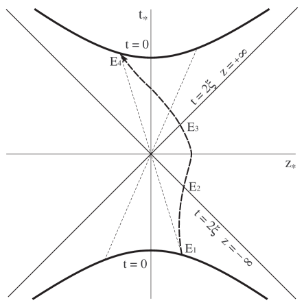
Figure 7: A hypothetical test particle starts its movement at the event $E_{1}$, i.e., at $t=0$, and arrives at $t=2\xi$ and $z=-\infty$, at event $E_{2}$. It re-enters into the interior region at event $E_{3}$, corresponding to $t=2\xi$ and $z=+\infty$, ending up in the spacelike singularity at $t=0$, at event $E_{4}$. As viewed from an interior observer the test particle exits the interior region, at $t=2\xi$ and $z=-\infty$, to reappear instantaneously at $t=2\xi$, at the positive side of the $z$ axis. According to the point of view of the interior observer, no time has elapsed during the test particle’s excursion in the exterior region.

VII Summary and discussion

The Schwarzschild solution has played a fundamental conceptual role in general relativity, and beyond, for instance, regarding event horizons, spacetime singularities and aspects of quantum field theory in curved spacetimes. In this work, we have provided a brief pedagogical review and further analyzed the interior Schwarzschild solution. Firstly, by deducing the interior metric by considering time-dependent metric fields, we have analyze the interior region, without the prejudices inherited from the exterior region. With this geometry at hand, we have payed close attention to several respective cosmological interpretations, and addressed some of the difficulties associated to spacetimes singularities. Secondly, we have deduced the conserved quantities of null and timelike geodesics, and discussed several particular cases in some detail. Finally, we examined the Eddington-Finkelstein and Kruskal coordinates directly from the interior solution.

A black hole is believed to have formed from the gravitational collapse of a massive body. However, events occurring in the interior of the event horizon are not observable for an exterior observer, and one may argue that relatively to the latter, black holes are not relevant physical objects Narlikar . Although the event horizon exists for exterior observers, all events in the range $r>2M$ are accessible to the interior observers. If one looks at the interior geometry as a continuation of the exterior static solution, one comes across some extremely interesting conceptual difficulties, that question the very concept of a black hole. For instance, while for the exterior observer, infalling particles end up at a central singularity at $r=0$, from the interior point of view, the proper distance along the $z-$direction increases, showing the existence of a cigar-like singularity. The latter singularity is a spacelike hypersurface, and the test particles are not directed towards a privileged point, however, in order to not violate causality they are directed along a temporal direction from $t=2\xi$ to $t=0$. A curious behavior relatively to an interior observer is also verified, as all infalling particles crossing the event horizon, occur simultaneously at $t=2\xi$. In this context, the Eddington-Finkelstein and Kruskal transformations do indeed solve the coordinate singularity at $r=2M$, but do not solve the problems associated with the inversion of the $r$ and $t$ coordinates. Assuming that $r$ is a temporal coordinate for $r<2M$, also signifies giving it a determined direction and duration, i.e., the black hole, or for that matter a white hole, possesses a finite coordinate temporal duration. However, the exterior geometry is static, and once created does not disappear.

An interesting feature relatively to the interior geometry is the issue of proper distances. The proper distance between two particles at rest separated by a constant $\Delta z$, decreases along the $z-$direction as coordinate time flows from $t=0$ to $t=2\xi$, and increases as coordinate time flows backwards from $t=2\xi$ to $t=0$. In counterpart, the proper distance between two simultaneous events along a spatial trajectory with $dz=0$ and $\theta=\pi/2$, increases as $t$ varies from $t=0$ to $t=2\xi$, and decreases when the temporal coordinate runs backwards from $t=2\xi$ to $t=0$. Another surprising result, considering the interior point of view, is that the trajectories of particles at rest are geodesics, contrary to the exterior where particles at rest are necessarily accelerated. This fact is due to the non-static character of the interior geometry.

In this work, we have addressed some conceptual difficulties related to the notion of black holes. The solutions that do away with the interior singularity and the event horizon Mazur ; gravastars ; Dymnikova ; darkstars , although interesting in themselves, sweep the inherent conceptual difficulties of black holes under the rug. In concluding, we note that the interior structure of realistic black holes have not been satisfactorily determined, and are still open to considerable debate.

References

- (1) J. R. Oppenheimer and H. Snyder, “On Continued Gravitational Contraction,” Phys. Rev. 56, 455 (1939).
- (2) K. Schwarzschild, “Uber das Gravitationsfeld einer Kugel aus inkompressibler Flussigkeit nach der Einsteinschen Theorie,” Sitzber. Deut. Akad. Wiss. Berlin, Kl. Math.-Phys. Tech., 424-434 (1916); R. C. Tolman, “Static solutions of Einstein’s field equations for spheres of fluid,” Phys. Rev. 55, 364 (1939); J. R. Oppenheimer and G. Volkoff, “On massive neutron cores,” Phys. Rev. 55, 374 (1939).
- (3) K. S. Thorne, R. H. Price and D. A. Macdonald (editors) Black holes: The membrane paradigm (Yale University Press, New Haven and London).
- (4) Ya. B. Zel’dovich and I. D. Novikov, Relativistic Astrophysics, The University of Chicago Press, Chicago, Illinois (1971).
- (5) R. Penrose, “Gravitational Collapse: The Role of General Relativity,” Riv. Nuovo Vimento Soc. Ital. Fis. 1, 252 (1969).
- (6) J. V. Narlikar and T. Padmanabhan, “The Schwarzschild solution: Some conceptual difficulties,” Found. Phys. 18, 659-668 (1988).
- (7) V. Sabbata, M. Pavsic and E. Recami, “Black holes and tachyons,” Lett. Nuov. Cim. 19, 441-451 (1977); R. Goldoni, “Black and white holes,” Gen. Rel. Grav. 1, 103-113 (1975).
- (8) A. I. Janis, “Note on motion in the Schwarschild field,” Phys. Rev. D 8, 2360 (1973); A. I. Janis, “Motion in the Schwarschild field: A reply,” Phys. Rev. D 15, 3068 (1977).
- (9) P. Crawford and I. Tereno, “Generalized observers and velocity measurements in general relativity,” Gen. Rel. Grav. 34, 2075 (2002) [arXiv:gr-qc/0111073].
- (10) V. J. Bolos, “Lightlike simultaneity, comoving observers and distances in general relativity,” Journ. Geom. Phys. 56, 813-829 (2006) [arXiv:gr-qc/0501085]; V. J. Bolos, “Intrinsic definitions of ‘relative velocity’ in general relativity,” [arXiv:gr-qc/0506032].
- (11) J. Earman, “Tolerance for spacetime singularities,” Found. Phys. 26, 623-640 (1996).
- (12) C. Misner, “Absolute Zero of Time,” Phys. Rev. 186, 1328 (1969).
- (13) P. O. Mazur and E. Mottola, “Gravitational Condensate Stars: An Alternative to Black Holes,” [arXiv:gr-qc/0109035]; P. O. Mazur and E. Mottola, “Gravitational Vacuum Condensate Stars,” Proc. Nat. Acad. Sci. 111, 9545 (2004) [arXiv:gr-qc/0407075]; G. Chapline, E. Hohlfeld, R. B. Laughlin and D. I. Santiago, “Quantum Phase Transitions and the Breakdown of Classical General Relativity,” Int. J. Mod. Phys. A 18 3587-3590 (2003) [arXiv:gr-qc/0012094].
- (14) M. Visser and D. L. Wiltshire, “Stable gravastars - an alternative to black holes?,” Class. Quant. Grav. 21 1135 (2004) [arXiv:gr-qc/0310107]; C. Cattoen, T. Faber and M. Visser, “Gravastars must have anisotropic pressures,” Class. Quant. Grav. 22 4189-4202 (2005) [arXiv:gr-qc/0505137]; N. Bilić, G. B. Tupper and R. D. Viollier, “Born-Infeld phantom gravastars,” JCAP 0602 013 (2006) [arXiv:astro-ph/0503427].
- (15) I. Dymnikova, “Vacuum nonsingular black hole,” Gen. Rel. Grav. 24, 235 (1992); I. Dymnikova, “Spherically symmetric space-time with the regular de Sitter center,” Int. J. Mod. Phys. D 12, 1015-1034 (2003) [arXiv:gr-qc/0304110]; I. Dymnikova and E. Galaktionov, “Stability of a vacuum nonsingular black hole,” Class. Quant. Grav. 22, 2331-2358 (2005) [arXiv:gr-qc/0409049].
- (16) G. Chapline, “Dark energy stars,” [arXiv:astro-ph/0503200]; F. S. N. Lobo, “Stable dark energy stars,” Class. Quant. Grav. 23, 1525 (2006) [arXiv:astro-ph/0508115].
- (17) M. A. Abramowicz, W. Kluzniak and J. P. Lasota, “No observational proof of the black-hole event-horizon,” Astron. Astrophys. 396 L31 (2002) [arXiv:astro-ph/0207270].
- (18) R. Kantowski and R. K. Sachs, “Some spatially homogeneous anisotropic relativistic cosmological models,” Journ. Math. Phys. 7, 443-445 (1966); C. B. Collins, “Global strucutre of the ‘Kantowski-Sachs’ cosmological models,” Journ. Math. Phys. 18, 2116-2124 (1977).
- (19) D. N. Vollick, “Anisotropic Born-Infeld Cosmologies,” Gen. Rel. Grav. 35, 1511 (2003) [arXiv:hep-th/0102187]; D. N. Vollick, “Black hole and cosmological space-times in Born-Infeld-Einstein theory,” [arXiv:gr-qc/0601136].
- (20) R. Doran, F. S. N. Lobo and P. Crawford, “Cosmological applications of the interior Schwarzschild solution,” (in preparation).
- (21) D. A. Easson and R. H. Brandenberger, “Universe generation from black hole interiors,” JHEP 0106, 024 (2001) [arXiv:hep-th/0103019].
- (22) R. W. Brehme, “Inside the black hole,” Am. J. Phys. 45, 423 (1977).
- (23) A. Karlhede, U. Lindström and J. E. Aman, “A Note on a Local Effect at the Schwarzschild Sphere,” Gen. Rel. Grav. 14, 569 (1982).
- (24) L. Landau and E. Lifschitz, The Classical Theory of Fields, Pergamon Press, New York, Fourth English Edition (1975).
- (25) V. V. Kiselev, “Radial geodesics as a microscopic origin of black hole entropy. I: Confined under the Schwarzschild horizon,” Phys. Rev. D 72 124011 (2005) [arXiv:gr-qc/0412090].
- (26) R. M. Wald, General Relativity, University of Chicago Press, Chicago, 1984.