Abstract

The double slit experiment (DSE) is known as an important cornerstone in the foundations of physical theories such as Quantum Mechanics and Special Relativity. A large number of different variants of it were designed and performed over the years. We perform and discuss here a new verion with the somewhat unexpected results of obtaining interference pattern from single-slit screen. We show using either the Brill’s version of the canonical formulation of general relativity or the linearized version of it that one may find corresponding and analogous situations in the framework of general relativity.

Pacs numbers:      42.25.Hz, 04.20.Gz, 04.30.-w, 04.20.Fy, 04.30.Nk

Keywords: Interference, Gravitational Waves, Trapped Surfaces

1 INTRODUCTION

There is no physical experiment which plays such an important historical role in the establishment and development of fundamental physical theories [2] such as the double slit experiment (DSE). It was first represented in 1803 by Young [3] as a desicive proof of the wave nature of light. Later, its interferometric character serves, through the Michelson-Morley experiment [4, 5], as the key trigger for the enunciation of the special relativity and the constancy of light velocity [5]. Still later, experimenting with some variants of the DSE (see the following paragraphs) has aroused fundamental problems and paradoxes which lead to a new physical understanding embodied in the laws of Quantum Mechanis ([6], see, especially, chapter 1 in [7]).

As known, the interference pattern resulting from the DSE [7, 8] appears even if the intensity of the passing light is decreased until an average of only one photon is in transit between source and double-slit screen [7]. From this one may conclude [7] that a single photon is capable of interfering with itself. Moreover, although each of the passing photons can go only through one of the slits the interference pattern appears only when both slits are open [7, 6, 9, 10]. In other words, as emphasized in [7, 9, 10], if the experiment is also designed, by either closing one slit or adding photons detectors at the slits (see Figure 3 in [7]), to supply the additional information of the exact slit through which each photon passes then the interference pattern disappears [7, 6, 9, 10]. This demonstrates the large influence of the observation itself upon the obtained results (see, for example, [9], for this influence in Quantum Mechanics and see [11] for this influence in relativity).

In order to isolate the real factors which determine the presence or absence of the interference pattern in the DSE we summarize here some versions of it [9, 10, 12] with particle detectors at the slits.

Experiments: The particle detectors are;

$(a)$ Turned-on and the data about the exact routes passed by the photons recorded and used during the experiment.

$(b)$ Turned off and, therefore, no data were recorded and used during the experiment.

$(c_{1})$ Turned on but the observer does not bother to record the count at the slits.

$(c_{2})$ Turned on and also recording the count at the slits but this information is thrown and not used during the experiment.

$(d)$ Turned-on and also recording the supplied information but it is mixed with other unrelated data so that the observer prepares some program which analyzes the combined information in either one of the two following ways;

$(d_{1})$ The unrelated data are removed in which case one remains with the real data from the detectors.

$(d_{2})$ Keeping the whole mixed-up information so the true data from the detectors are not available.

Results: For final analysis of $(b),\ (c_{1}),\ (c_{2}),\ (d_{2})$ an interference pattern appears and for $(a),\ (d_{1})$ no such pattern is seen. We note that for $(a)$, $(d_{1})$ the optical pattern shown on the screen is separated into two patterns [9, 10, 12] each of them is of the single-slit experiment (SSE) kind and corresponds to the slit which is in line with it. That is, there exists no interference of any photon from one slit with any other photon from the other slit so that each of the two patterns is formed from the diffraction of the particles which pass through the slit in line with it as schematically shown in Figure 3.

One may realize from $(b)$, $(c_{1})$, $(c_{2})$ and $(d_{2})$ that even the determination and recording of the exact routes of the particles through the double-slit screen are not enough for cancelling the interference pattern if, as mentioned, these data from the detectors are not included in the experiment itself [7]. It can also be seen from the results of $(d_{1})$ and $(d_{2})$ that the inclusion of these data in the DSE may be performed even years after completing the passage through the slits (of course, before obtaining the optical pattern on the photosensitive screen) which constitutes the known delayed choice experiment [9, 12]. That is, the important factor which determines the form of the obtained optical pattern is the use (or not), during the DSE, of the information about the routes of the photons through the slits. Moreover, as seen in the optical literature [8], this is valid for any multiple-slit screen. That is, any such screen may demonstrate either the interference pattern of the DSE kind (as in Figure 1) if the data about the routes through slite are not used during the experiment or a number of diffraction patterns each of them of the SSE kind (see Figure 2) if these data are used. The number of these SSE’s diffraction patterns equals the number of slits as seen, for example, in Figure 4 for the four-slit screen where the data about routes are used during the experiment. The only difference between the interference pattern of the DSE and that of any other $n$-slit pattern is that the larger is $n$ the thinner become the fringes of this pattern [8].

We show, through actual experiments, that the noted conditions of using or not using the data about the photons routes which, respectively, entail diffraction or interference patterns are valid not only for the double or any other multiple-slit screen but also for the SSE. Note that for any $n$-slit screen, where $n\geq 2$, the mentioned data about routes may sum, for a large number of photons, to a huge amount of information whereas for the SSE these data involve only one single piece which is that all the photons pass only through that slit. Thus, we show that if this single data is not used during the experiment then the expected single-slit diffraction pattern does not appear.

It should be noted in this context that up to now the very nature of the employed screen, if it is single, double or multiple-slit, is always known and used during the experiment. But unlike the double and any other multiple-slit experiments for which one may know and, therefore, use during the experiment the datum about the number of slits without using the data about the routes of the photons through them for the SSE case they, actually, lead to each other. This is because if one knows and, therefore, use during the experiment the datum that he is employing single-slit screen then he, automatically, also knows and use the datum that all photons pass through that slit and vice versa.

Suppose, now, that the observer activates a single-slit screen without knowing it and, therefore, the information related to the single route of all the photons can not be used during the experiment. We show that in this case, and under the special conditions described in Section II, the resulting pattern is that of interference as demonstrated in the appended pictures [13]. That is, instead of obtaining the diffraction pattern, shown in Figure 2, which is typical of SSE we have obtained the interference pattern, shown in Figure 1, which is characteristic of $n$-slit screen ( $n\geq 2$). That is, one may conclude for any $n$-slit screen, where $n\geq 1$, that if one uses the data about the routes then one obtains $n$ diffraction patterns where $n$ is the number of slits as shown, for example, in Figure 2 for $n=1$ and in Figures 3-4 for $n=2$ and $n=4$. If, however, these data are not taken into account during the experiment then the obtained pattern for any $n$-slit screen, even for $n=1$, is the interference one shown in Figure 1. In other words, for all $n$-slit screens, where $n\geq 1$, changing the situation from using during the experiment the data about the photon routes to not using them amounts to changing these routes from being densely and continuously arrayed in the forward directions ($m=0$) to being fringed and striped.

We show in this work that this formation of periodic fringes and stripes may also be found as geodesics changes in at least two theoretical branches of the general relativity theory. As known, using the equivalence principle [5, 14, 15] one may discuss any physical event as either occuring in a flat spacetime with physical interactions or resulting from a curved spacetime [5, 14, 15] with no such interactions. Thus, the mentioned change of the photon routes, from the continuous diffraction type (in the neighbourhood of the order $m=0$) to the fringed interference one, may be, theoretically, paralleled to corresponding situations in general relativity [5, 14, 15].

Note that one may argue that the mentioned DSE results, detaily described in Section II, should be exclusively discussed in pure quantum mechanical terms without having to invoke any general relativity idea. We answer to this that the relativistic discussion here is not suggested as some kind of explanation or interpretation of this DSE. Our aim in this discussion is to point out that corresponding and parallel situations may also, as mentioned, be encountered in the framework of general relativity. That is, one may, theoretically, find formations of fringed and nonfringed trapped surfaces which are related to the same kind of GW (either the Brill or plane GW’s) as those found with the same kind of optical screen (see Figures 7-8).

As known [5, 14, 15] geodesics changes are related in the general relativity to corresponding changes in the geometry of the surrounding spacetime which are, especially, tracked to the presence of gravitational waves (GW) [14, 15, 16]. Moreover, if these GW are strong enough they may entail corresponding and lasting changes in the form of the relevant geodesics which stay long after the generating GW disappear. As mentioned, the noted changes in the photon routes result only from considering (or not) during the experiment the data regarding these routes and not from any other force. Thus, a suitable parallel gravitational situation is related more to the pure source-free GW’s [14, 17, 18, 19] than to the matter-sourced ones [14, 15, 16]. Accordingly, we pay special attention in the following to these source-free gravitational fields which constitute solutions to the Einstein vacuum field equations [5, 14, 15] and propagate in vacuum as pure source-free GW’s [14, 17, 18, 20] with no involvement of matter.

As representatives of these source-free radiation we consider the (1) Brill GW’s [17, 18, 20, 21] and (2) the plane GW’s in the linearized version of general relativity. The later kind is chosen because it is discussed in the almost flat metric which is similar to the flat metric of the mentioned optical experiments. Moreover, it has been shown [30, 31] that, like the electromagnetic (EM) $n$-slit experiments, the plane GW in the linearized version of general relativity have, under special conditions, properties which make it capable of interfering with other GW’s. Both of these GW change, if they are strong enough, the surrounding spacetime and its topology [22, 23] which, naturally, entail also changes of geodesics. The new changed spacetime is, theoretically, represented, in the spacetime region traversed by these GW’s, by trapped surfaces [14, 18, 24, 25, 26, 21] which have the same intrinsic geometry as that of the generating GW. One may, especially, count two different kinds of these surfaces; (1) the singular trapped ones [18, 26, 21, 27, 28] and (2) the nonsingular ones [25] which are related to the regular and asymptotically flat initial data [14, 18, 17, 29] in vacuum. Note that as [30] interference patterns and holographic images result from interfering electromagnetic waves so trapped surfaces result also from interfering GW’s.

In Section II we represent a detailed account of the experiment from which we obtain, under suitable conditions, interference fringed pattern from single-slit screen. In Section III we have shown that one may obtain similar fringed geodesics by beginning from the Brill’s metrics and use the terms and terminology related to it. We have, also, calculated the corresponding fringed trapped surface which is formed from this Brill’s pure radiation. The trapped surface, without fringing, resulting from the Brill GW’s have been calculated in [18] and were represented, for comparison and completness, in Appendix A. In this Appendix we have also represent a short review of the ADM canonical formulation [29, 14] of general relativity and the specific conditions which lead to the Brill’s source-free GW’s. In Section IV we have calculated the fringed trapped surface obtained from plane GW’s by using the approximate linearized general relativity [14]. The plane GW’s in the framework of this approximate theory and the resulting trapped surfaces, without fringing, have been detaily calculated in [30] and were represented, for comparison and completness, in Appendix B. We discuss and summarize the main results in a Concluding Remarks Section.

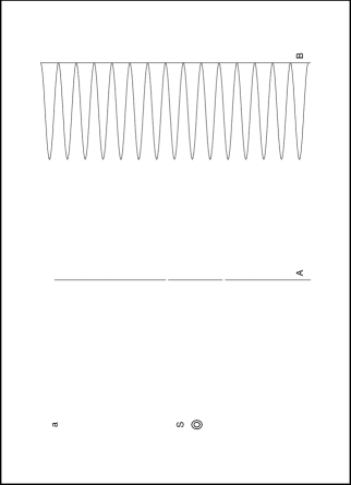
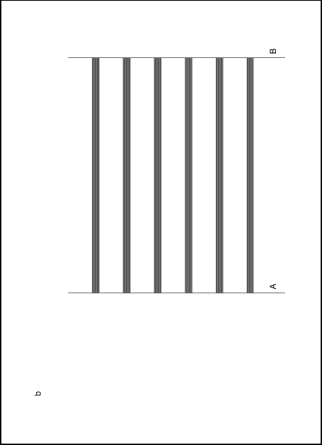
Figure 1: A schematic representation of the DSE, including the light source $S$, is shown at the left Subfigure $a$ where the data about the routes through slits are not used during the experiment. The interference pattern resulting from the optical path difference between the rays from the two slits at screen $A$ is shown on the photosensitive screen $B$. At the right Subfigure $b$ one may see the corresponding routes traversed by the photons between the two screens.

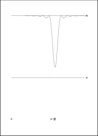
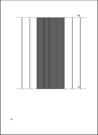
Figure 2: A schematic representation of the SSE, including the light source $S$, is shown at the left Subfigure $a$ where the observer knows and, therefore, uses during the experiment the datum about the nature of screen. The diffraction pattern resulting from the optical path difference between rays from same slit at screen $A$ is shown on the photosensitive screen $B$. At the right Subfigure $b$ one may see the corresponding routes traversed by the photons between the two screens where the most traversed route is that in the forward direction ($m=0$).

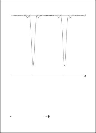
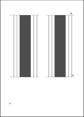
Figure 3: At the left Subfigure $a$ we see the optical pattern obtained from the double-slit screen when the routes of the photons through the slits are recorded and taken into accound during the experiment. One have here no interference between rays from the two slits but two separate diffraction patterns each composed by the photons passed through the slit in line with it. At the right Subfigure $b$ we see the form of the routes between the screens where most photon pass in the two forward directions.

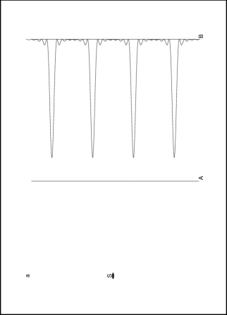
Figure 4: At the left Subfigure $a$ we see the optical pattern obtained from the four-slit screen when the routes of the photons through the slits are recorded and taken into accound during the experiment. One have here no interference between rays from any two slits but four separate diffraction patterns each composed by the photons passed through the slit in line with it. At the right Subfigure $b$ we see the form of the routes between the screens where most photon pass in the four forward directions.

2 Obtaining interference pattern from SSE

The experimental set-up for the variant of the DSE discussed here includes a laser pointer as light source and 30 mirrors. The laser pointer acts as a strong monochromatic red light source with wavelength in the 650-680 $nm$ range and output of less than 1 $mW$. The mirrors were prefered to serve as double and single slit screens because it is easy to inscribe on their coated sides very narrow slits (scratchs). Thus, using double edge razor blades two narrow slits of about $0.3\ mm$ wide were cut in the coated side of each of them where the distances between the slits varied in the range of $1-4\ mm$. Twenty nine (29) mirrors were prepared to serve as real double slits screens and in the remaining mirror one slit was real and the second was spurious and superficially cut so that it was still opaque. This is done so that when the observer looks at this mirror from some distance he would not differentiate between it and the other real two-slit ones.

In Figure 5 one may see a photograph of the actual arrangement of the experiment. This figure as well as Figures 6-8 are real pictures photographed by a digital camera [13]. In Figure 5 one may see at the front the laser pointer mounted upon a white rectangular box. As seen, this laser pointer is hold by two binder clips which serve the twofold purpose of conveniently directing it towards the back of the mirror-screen and also of pressing its operating button so as to activate it. At the back of the Figure one may see a second rectangular box upon which one mirror (of the available 30) is mounted with the help of a second pair of binder clips. One may also see at the back of the mirror the real or spurious double slit and the red laser ray from the pressed laser pointer. Moreover, with a larger resolution one may even discern the red optical pattern at the white wall behind the mirror. At the right one may see inside another rectangular box the operated mirrors. In Figure 6 one may see a typical picture of the optical interference pattern obtained from one of the 29 real double-slit mirrors where the nature of this mirror is known and used during the experiment but not the data about the routes of the photons through the slits. In Figure 7 we show two typical photographs of the optical diffraction pattern obtained from the faked double-slit mirror when its true nature, that it is single-slit, is used during the experiment. The left picture was photographed by taking a longer distance between the mirror and the white wall compared to the distance used for the right picture.

Using random number generator the observer begins the experiment by randomely picking one mirror from the available 30 without knowing if he choose one of the real double-slits or the faked one where the probability to choose the former is $\frac{29}{30}=0.97$ and that for picking the latter is $\frac{1}{30}=0.033$. He then point the laser pointer from a distance of about 1 meter at the apparent double slits in the coated side of the mirror and look at the resulting light pattern on the white wall situated 1.75 meters from the mirror (see Figure 5). The obtained light pattern is expected to be either that of the interference type as in Figure 1 in case the activated screen was one of the real double slit mirrors or that of the diffraction form of Figure 2 if this screen was the spurious one. After obtaining the optical pattern upon the white wall the observer checks the operated screen to see if it is one of the real double-slit mirrors or the faked one. Thus, if it is found to be one of the true double-slit mirrors it is returned to the pile of 30 mirrors from which another one (which may be the former) was randomely chosen for a new experiment of the type just described. This repetition was stopped only when the involved screen was found to be the spurious one.

Now, since the chance of randomely picking the faked screen is only $0.033$ whereas that for chosing the real one is $0.97$ one, naturally, have to repeat the described experiment a large number of times until the spurious screen was found. Thus, this experiment was, actually, repeated 228 times over several weeks and for each of these experiments we have first obtained interference pattern and then found that the activated screen was one of the 29 real double-slit screens as expected. The 229-th experiment began, as its predecessors, without knowing and, therefore, without using the true nature of the involved screen and, as before, the obtained light pattern was of the interference type but upon looking closely at the relevant screen it has, somewhat unexpectedly, turned out to be the spurious one which is, actually, a single slit. That is, interference pattern, which typically result from $n$-slit screen ($n\geq 2$) was, actually, obtained from single-slit one.

In order to be sure of this result a new series of these experiments was again repeated but this time each optical pattern is photographed by a digital camera [13] before checking the true nature of the activated screen. As before, hundreds of them (216) were performed over several weeks before the faked double-slit screen were turned up at the 217-th experiment. As for the former series of experiments the finding of this actually single-slit screen was preceded by obtaining the $n$-slit interference pattern ($n\geq 2$) and not the expected single-slit diffraction one. This time, unlike the former series, all the obtained 217 optical patterns were photographed before checking the nature of the employed screen. A photograph of the optical pattern resulting from the 217-th experiment is shown in Figure 8 and one may see that it is of the interference pattern kind as realized when comparing it to Figure 6 which shows the optical pattern obtained from a real double-slit screen.

Figure 5: This figure is a digital camera photograph of the arrangement used to perform the experiment described in Section II. At the front one may see on a white box the red laser pointer hold by two binding clips. At the back one may see on another box the slitted mirror which is also hold by another pair of binding clips. The red laser ray from the pointer is shown at the back of the mirror and with a larger resolution one may even discern the optical pattern on the white wall. At the right one may see in another box the ensemble of mirrors used.

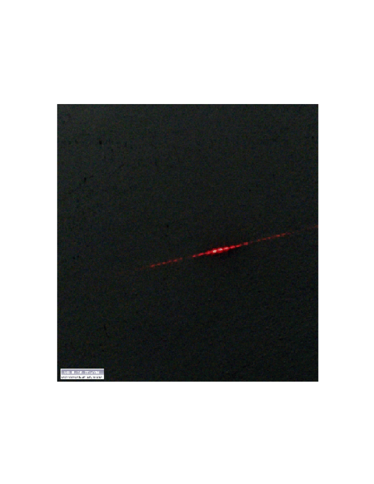
Figure 6: The optical interference pattern obtained from one of the 29 real double-slit mirrors where the nature of this screen is known but not the data about the routes through the slits.

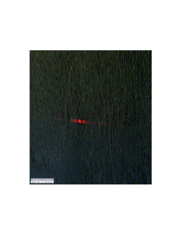
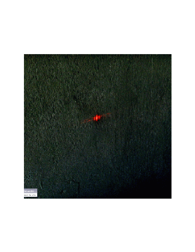
Figure 7: At the left and right Subfigures we see photographs of the optical single-slit diffraction pattern taken at the start of the experiment from the spurious double-slit screen where the true nature of this screen was known and used during the experiment. The distance between the mirror and wall, used for obtaining the optical pattern of the left picture, was larger compared to that used for the right picture.

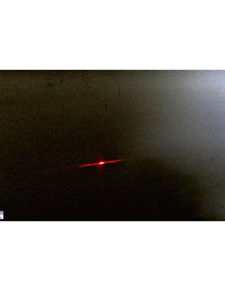
Figure 8: This figure is a photograph of the optical interference pattern obtained from the spurious double-slit screen where the true nature of this screen was not known and, therefore, not used during the experiment. Note the similarity of this pattern, actually obtained from single-slit screen, to that of Figure 6 which was obtained from one of the real double-slit screens. Comparing this photograph to those of Figure 7, which are obtained from the same screen, one may realize that the use (or not) during the experiment of the relevant data is the important factor which determines the obtained optical pattern.

Analysing the former results one may conclude that performing these experiments under the conditions of not knowing the nature of screen and, therefore, not using during the experiments the data about the routes through the slits changes the form of these routes from the diffraction pattern of Figure 2, $b$ to the $n$-slit interference one ($n\geq 2$) shown in Figure 1 ,$b$. This outcome for the SSE together with the mentioned results obtained for any other $n$-slit screen ($n\geq 2$) led one to conclude that interference pattern is obtained for any $n$-slit screen, even for $n=1$, so long as the mentioned data were not used during the experiment. When, however, these data are used during the experiment one obtains for such $n$-slit screen ($n\geq 1$) $n$ diffraction patterns each of them of the SSE kind shown in Figure 2. In other words, considering the central region around the order $m=0$, one may realize that, when the noted data are not used during the experiments, this region becomes striped and fringed compared to the nonfringed form it has when these data are used. That is, an interval between photon routes, which were zero in the region around $m=0$ when the noted data were used (see Figures 2-4), has been formed when these data were not used (see Figure 1). We calculate in the following the length of this interval which is shown in Figure 9 between neighbouring maxima. The path difference between two rays from the two slits is shown at the left of Figure 9. Thus, denoting by ${\cal B}$ and ${\cal D}$ the respective bright and dark fringes upon the photosensitive screen one may use Figure 9 and write these path differences for the DSE as [8]

$$d\sin(w)_{{\cal B}}=m\lambda$$ (1)

$$d\sin(w)_{{\cal D}}=(m+\frac{1}{2})\lambda$$

As shown in Figure 9, $d$ and $d\sin(w)$ respectively denote the interval between the two slits and the path difference between the two interfering waves. By $\lambda$ and $m=0,1,2,....$ we denote the wavelength of the light from the source and the order of interference. For the single slit experiment (SSE) one may use the following expressions [8]

$$b\sin(w)_{{\cal B}}=m\lambda$$ (2)

$$b\sin(w)_{{\cal D}}=(m+\frac{1}{2})\lambda,$$

where $b$ is the length of the slit and $b\sin(w)$ is the path difference between rays diffracted from the ends of the slit. That is, the locations of the different maxima and minima do not result from any interference but from diffraction through the single slit. As a result, the maximum intensity for the order $m=0$ is greater by several order of magnitudes from the corresponding maxima shown for the orders $m=1,2,...$ (see Figure 2) and from those of the DSE. That is, most photons which diffract through the single slit propagate parallel to each other in the forward straight direction which explains the large intensity for the order $m=0$.

In Figure 9 we show the two ordered maxima $m=0$ and $m=1$, denoted in the following by $m_{0}$ and $m_{1}$, and calculate the interval between them by considering the right angled triangle build from the sides $m_{0}-x_{1}$, $g$ and $f$ where $x_{1}$ denotes the first minimum. From this triangle one obtain $\tan(w)=\frac{(m_{0}-x_{1})}{g}$ so that the sought-for length $\Delta(w)=m_{0}-m_{1}$ is

$$\Delta(w)=m_{0}-m_{1}=2g\tan(w)$$ (3)

As noted, the changed photon routes may be paralleled to corresponding geodesics changes. These changes are extensively discussed [5, 14, 15, 33] in the framework of general relativity (see, especially, the annotated references in [14]) as resulting from corresponding spacetime changes. The later changes are, especially, tracked to GW’s [16] whose intrinsic spacetime geometry [28] is imprinted upon the traversed spacetime. As mentioned, we pay special attention to the more appropriate source-free GW’s and consider the Brill’s and plane GW’s (we may also discuss the Kuchar’s cylindrical source-free GW’s [14, 34]).

Thus, as for the optical slitted-screens in which one may either use during the experiments the data about the routes through the slits (which result in obtaining diffraction patterns) or not using these data (which result, for any $n$-slit ecreen ($n\geq 1$), in obtaining fringed interference pattern) one may, likewise, discern two similar gravitational states. One state may be characterized by some assumed spacetime metrics such as the Brill’s or the almost flat metrics which is used in discussing plane GW’s. The second gravitational state is characterized by a metrics which, actually, is the fringing of the former in a manner similar to the stripes of the interference pattern which may be regarded as the fringing, especially, in the neighbourhood of the orders $m=0$, of the diffraction patterns of Figures 2-4. The Brill’s metrics and its corresponding nonfringed trapped surface [18] is reviewed in Appendix A and the almost flat metrics with the relevant nonfringed trapped surface [30] is represented in Appendix B. The fringed trapped surfaces is discussed in the following section for the Brill’s GW and in Section IV for the almost flat plane GW’s.

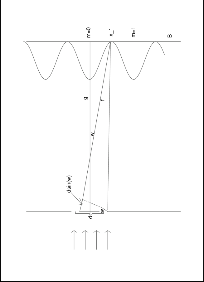
Figure 9: A schematic representation of the double-slit array, used to obtain interference patterns, is shown. The path difference $d\sin(\phi)$ and the sinusoidal interference form are shown. Using this figure one may obtain Eq (3) for the interval between the orders $m=0$ and $m=1$.

3 The fringed trapped surface resulting from the Brill GW’s

The source-free Brill GW’s are discussed in the framework of the ADM formalism [14, 29]. In this canonical formulation of general relativity one, generally, consider the simplified case of time and axial symmetries and no rotation [17, 18, 20]. Under these conditions one finds a solution [17, 18, 20] to the Einstein vacuum field equations which represents, as mentioned, pure source-free gravitational wave with positive energy [17, 18, 20, 21]. A short review of the ADM canonical theory [14] with the former conditions is represented in Appendix $A$. Strong Brill GW’s are involved with the appearance of a marginally trapped surfaces which are equivalent, for the time-symmetric condition discussed here, to minimal area surfaces [18]. These surfaces may be represented in a cartesian coordinates by using embedding diagrams of them [14, 18]. As known [14, 18], to embed the whole surface is difficult so one, generally, resort to the task of embedding a plane through the equator which is simpler due to the assumed rotational symmetry.

As mentioned, we have obtained for any $n$-slit screen, even for $n=1$ as described in Section II, an interference pattern which are periodically alternating sequence of light and dark bands (see Figure 1, $b$) where the bright bands allow photons to pass along them and the dark ones do not allow them. Using the equivalence principle these alternating fringes may, as mentioned, be discussed as periodically alternating bands of geodesics. That is, the optical bright bands correspond to strong curvature [5, 14, 15] geodesics and the optical dark bands to the weak curvature ones. As noted, these alternating bands of strong and weak curvatures may be considered as forming a trapped fringed surface which, theoretically, can be embedded in an Euclidean space [14, 18, 24]. The embedding procedure may, analytically, be expressed by requiring the metric of the equator [18] to be equal to that of a rotation surface (in Euclidean space) which is formed from a periodic alternating allowed and disallowed bands. That is, one may write

$$x^{B}=F^{B}(\rho,\phi)\cdot\cos(\phi)$$

$$y^{B}=F^{B}(\rho,\phi)\cdot\sin(\phi)$$ (4)

$$z^{B}=h^{B}(\rho),$$

where the function $h^{B}(\rho)$ does not depend upon the variable $\phi$ and the superscript $B$ denote that we refer to the Brill source-free case. The function $F^{B}(\rho,\phi)$ may be written as the following products

$$F^{B}(\rho,\phi)=f^{B}(\rho)\cdot M^{B}(\phi),$$ (5)

where the function $M^{B}(\phi)$ is introduced to ensure the mentioned periodic fringing and is defined as

$$M^{B}(\phi)=\left\{\begin{array}[]{ll}1&\ \ {\rm for}-\pi\leq\phi\leq-\frac{\pi}{2}\\ 0&\ \ {\rm for}-\frac{\pi}{2}<\phi<\frac{\pi}{2}\\ 1&\ \ {\rm for}\frac{\pi}{2}\leq\phi\leq\pi\end{array}\right.$$ (6)

As seen, the periodic function $M^{B}(\phi)$, which is shown in Figure 10, is piecewise monotonic and bounded on the interval $(-\pi,\pi)$ and so it can be expanded in a Fourier series [35, 36]. Thus, using the Fourier analysis [35, 36] one may determine the Fourier coefficients as

$$a^{B}_{0}=\frac{1}{\pi}\int_{-\pi}^{\pi}M^{B}(\phi)d\phi=\frac{1}{\pi}\bigl{(}\int_{-\pi}^{-\frac{\pi}{2}}1d\phi+\int_{-\frac{\pi}{2}}^{\frac{\pi}{2}}0d\phi+\int_{\frac{\pi}{2}}^{\pi}1d\phi\bigr{)}=\frac{1}{\pi}\pi=1$$

$$a^{B}_{k}=\frac{1}{\pi}\int_{-\pi}^{\pi}M^{B}(\phi)\cos(k\phi)d\phi=\frac{1}{\pi}\int_{-\pi}^{-\frac{\pi}{2}}1\cos(k\phi)d\phi+$$

$$+\frac{1}{\pi}\int_{\frac{\pi}{2}}^{\pi}1\cos(k\phi)d\phi=\frac{1}{\pi}\bigl{(}\frac{\sin(k\phi)}{k}\bigr{)}{\Large|}^{-\frac{\pi}{2}}_{-\pi}+\frac{1}{\pi}\bigl{(}\frac{\sin(k\phi)}{k}\bigr{)}{\Large|}^{\pi}_{\frac{\pi}{2}}=$$

$$=-\frac{2}{\pi k}\sin(k\frac{\pi}{2})=\left\{\begin{array}[]{ll}0&{\rm for\ k\ even}\\ -\frac{2}{\pi k}&{\rm for\ k\ odd\ and\ k=4n-3}\\ \frac{2}{\pi k}&{\rm for\ k\ odd\ and\ k=4n-1}\end{array}\right.$$ (10)

$$b^{B}_{k}=\frac{1}{\pi}\int_{-\pi}^{\pi}M^{B}(\phi)\sin(k\phi)d\phi=\frac{1}{\pi}\int_{-\pi}^{-\frac{\pi}{2}}1\sin(k\phi)d\phi+\frac{1}{\pi}\int_{\frac{\pi}{2}}^{\pi}1\sin(k\phi)d\phi=$$

$$=-\frac{1}{\pi}\bigl{(}\frac{\cos(k\phi)}{k}\bigr{)}{\Large|}^{-\frac{\pi}{2}}_{-\pi}-\frac{1}{\pi}\bigl{(}\frac{\cos(k\phi)}{k}\bigr{)}{\Large|}^{\pi}_{\frac{\pi}{2}}=0,$$

where $n=1,\ 2,\ 3,\ 4......$. From the last Eqs (6)-(10) one may write the function $M^{B}(\phi)$ as

$$M^{B}(\phi)=1-\frac{2}{\pi}\left(\frac{\cos(1\phi)}{1}+\frac{\cos(5\phi)}{5}+\ldots+\frac{\cos((4n-3)\phi)}{(4n-3)}+\ldots\right)+$$

$$+\frac{2}{\pi}\left(\frac{\cos(3\phi)}{3}+\frac{\cos(7\phi)}{7}+\dots+\frac{\cos((4n-1)\phi)}{(4n-1)}+\ldots\right)=$$ (11)

$$=1-\frac{2}{\pi}\left(\sum_{n=1}^{\infty}\frac{\cos((4n-3)\phi)}{(4n-3)}-\sum_{n=1}^{\infty}\frac{\cos((4n-1)\phi)}{(4n-1)}\right)$$

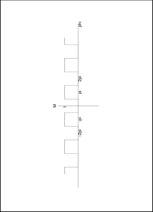
Figure 10: In this figure one may see the periodic function $M(\phi)$ from Eq (6).

Now, using Eqs (4)-(5) and following the discussion in [18] one may write for the metric on the equator

$$(ds^{B})^{2}=(dx^{B})^{2}+(dy^{B})^{2}+(dz^{B})^{2}=\biggl{(}(M^{B})^{2}(\phi)(f^{B})_{\rho}^{2}(\rho)+$$ (12)

$$+(h^{B})_{\rho}^{2}(\rho)\biggr{)}d\rho^{2}+(f^{B})^{2}(\rho)\biggl{(}M^{B})_{\phi}^{2}(\phi)+(M^{B})^{2}(\phi)\biggr{)}d\phi^{2}+$$

$$+4M^{B}(\phi)M^{B}_{\phi}(\phi)f^{B}_{\rho}(\rho)f^{B}(\rho)d\rho d\phi,$$

where $f^{B}_{\rho}(\rho),\ h^{B}_{\rho}(\rho)$ denote the respective derivatives of $f^{B}(\rho),\ h^{B}(\rho)$ with respect to $\rho$ and $M^{B}_{\phi}(\phi)$ is the derivative of $M^{B}(\phi)$ with respect to $\phi$. The metrics from Eq (12) is equated to the Brill’s one [17, 20, 18] which is represented in Appendix A. Note that for performing the mentioned embedding one consider [18] only the metrics on the equator [18] which is equated to the surface of rotation from Eqs (4) and also the metrics for the Brill GW’s is generally assumed for the norotation case [18] (see Appendix A). Thus, one obtains from this equating process

$$(ds^{B})^{2}=(dx^{B})^{2}+(dy^{B})^{2}+(dz^{B})^{2}=\biggl{(}(M^{B})^{2}(\phi)(f^{B})_{\rho}^{2}(\rho)+$$

$$+(h^{B})_{\rho}^{2}(\rho)\biggr{)}d\rho^{2}+f^{2}(\rho)\biggl{(}(M^{B})_{\phi}^{2}(\phi)+(M^{B})^{2}(\phi)\biggr{)}d\phi^{2}=$$ (13)

$$=g^{B}_{\rho\rho}d\rho^{2}+g^{B}_{\phi\phi}d\phi^{2}=\psi^{4}e^{2Aq}d\rho^{2}+\psi^{4}\rho^{2}d\phi^{2},$$

where $g^{B}_{\rho\rho}$ and $g^{B}_{\phi\phi}$ are the $(\rho\rho)$ and $(\phi\phi)$ components of the Brill metric tensor. For obtaining $F^{B}(\rho,\phi)$, $F^{B}_{\rho}(\rho,\phi)$ and $h^{B}(\rho)$ one equates the coefficients of $d\rho^{2}$ and $d\phi^{2}$ as follows

$$F^{B}(\rho,\phi)=f^{B}(\rho)M^{B}(\phi)=\frac{\rho\psi^{2}}{\sqrt{1+\frac{(M^{B})_{\phi}^{2}(\phi)}{(M^{B})^{2}(\phi)}}}$$

$$F^{B}_{\rho}(\rho,\phi)=f^{B}(\rho)_{\rho}M^{B}(\phi)=\frac{1}{\sqrt{1+\frac{(M^{B})_{\phi}^{2}(\phi)}{(M^{B})^{2}(\phi)}}}\left(\psi^{2}+2\rho\psi\psi_{\rho}\right)$$ (14)

$$h^{B}(\rho)=\int d\rho\biggl{(}\psi^{4}e^{2Aq}-(F^{B})_{\rho}^{2}(\rho,\phi)\biggr{)}^{\frac{1}{2}}=\int d\rho\biggl{(}\psi^{4}e^{2Aq}-(M^{B})^{2}(\phi)(f^{B})_{\rho}^{2}(\rho)\biggr{)}^{\frac{1}{2}}$$

The last expressions for $F^{B}(\rho,\phi)$, $F^{B}_{\rho}(\rho,\phi)$ and $h^{B}(\rho)$ define the embedded fringed surface $z(x,y)$ on the equator which has the same geometry as that of the time-symmetric Brill’s GW. These surfaces have the same general forms as those shown in Figure 11 for the nonfringed surfaces of Eqs ($A_{13}$) except that now, for appropriately representing Eqs (14), these surfaces should be periodically fringed.

Now, as done in Section II regarding the orders $m$ of the fringed interference pattern (see Eqs (1)-(3)) and the intervals between neighbouring maxima we also find here the orders and intervals related to the fringed trapped surface geometry resulting from the Brill GW’s. That is, realizing from Eq (6) and Figure 10 that any two neighbouring maximal or minimal bands, for which one respectively have $M^{B}(\phi)=1$ and $M^{B}(\phi)=0$, are separated by intervals of $\pm\pi$ one may denote the angles related to these ordered bands by $\phi_{m}=\phi_{0}\pm m\pi$ where $\phi_{0}$ corresponds to $m=0$. Note that for $m$ even (positive or negative) one always have $\cos(\phi_{m})=\cos(\phi_{0})$, $\sin(\phi_{m})=\sin(\phi_{0})$ and for $m$ odd (positive or negative) $\cos(\phi_{m})=-\cos(\phi_{0})$, $\sin(\phi_{m})=-\sin(\phi_{0})$. Also, one always have for any $m$, positive or negative, even or odd, $\cos(\phi_{m+1})=-\cos(\phi_{m})$, $\sin(\phi_{m+1})=-\sin(\phi_{m})$. Thus, remembering that the coordinates of the fringed trapped surfaces are given by Eqs (4) one may write in correspondence with Eqs (1)-(2)

$$x^{B}_{m}=F^{B}(\rho,\phi_{m})\cos(\phi_{m})=f^{B}(\rho)M^{B}(\phi_{m})\cos(\phi_{m})$$ (15)

$$y^{B}_{m}=F^{B}(\rho,\phi_{m})\sin(\phi_{m})=f^{B}(\rho)M^{B}(\phi_{m})\sin(\phi_{m}),$$

where for maximal bands one should have either $-\pi\leq\phi\leq-\frac{\pi}{2}$ or $\frac{\pi}{2}\leq\phi\leq\pi$ for which $M^{B}(\phi)=1$ (see Eq (6)) and for minimal bands $\phi$ should be from the range $-\frac{\pi}{2}<\phi<\frac{\pi}{2}$ for which $M^{B}(\phi)=0$ (see Eq (6)). Now, denoting the interval between two neighbouring $m$ orders in the fringed trapped surface geometry by $\Delta^{B}(\rho)$ and using the relations $\cos(\phi_{(m+1)})=-\cos(\phi_{m})$, $\sin(\phi_{(m+1)})=-\sin(\phi_{m})$ and $M^{B}(\phi_{(m+1)})+M^{B}(\phi_{m})=2$ (see Eq (11)) one may write in correspondence with Eq (3)

$$\Delta^{B}(\rho)=\sqrt{\left(x^{B}_{(m+1)}-x^{B}_{m}\right)^{2}+\left(y^{B}_{(m+1)}-y^{B}_{m}\right)^{2}}=$$

$$=\biggl{\{}\biggl{(}f^{B}(\rho)M^{B}(\phi_{m+1)})\cos(\phi_{(m+1)})-f^{B}(\rho)M^{B}(\phi_{m})\cos(\phi_{m})\biggr{)}^{2}+$$ (16)

$$+\biggl{(}f^{B}(\rho)M^{B}(\phi_{m+1)})\sin(\phi_{(m+1)})-f^{B}(\rho)M^{B}(\phi_{m})\sin(\phi_{m})\biggr{)}^{2}\biggr{\}}^{\frac{1}{2}}=$$

$$=\biggl{\{}(f^{B})^{2}(\rho)\biggl{(}M^{B}(\phi_{(m+1)})+M^{B}(\phi_{m})\biggr{)}^{2}\biggl{(}\cos^{2}(\phi_{m})+\sin^{2}(\phi_{m})\biggr{)}\biggr{\}}^{\frac{1}{2}}=$$

$$=2f^{B}(\rho)=\frac{2\rho\psi^{2}}{\sqrt{((M^{B})^{2}(\phi)+(M^{B})_{\phi}^{2}(\phi))}},$$

where the last result follows from the first of Eqs (14).

4 The fringed trapped surface resulting from the linearized plane GW’s

We, now, find, as for the Brill GW’s discussed in the former section, the required fringed trapped surface related to the linearized plane GW’s and begin by assuming, as in [18], that its metric is that of a surface of rotation $z(x,y)$ related to Euclidean space. That is, one may write

$$x^{P}=F^{P}(\rho,\phi)\cos(\phi)=f^{P}(\rho)M^{P}(\phi)\cos(\phi),$$

$$y^{P}=F^{P}(\rho,\phi)\sin(\phi)=f^{P}(\rho)M^{P}(\phi)\sin(\phi),$$ (17)

$$z^{P}=h^{P}(\rho),$$

where we have superscripted the quantities $F(\rho,\phi)$, $M(\phi)$, $f(\rho)$ and $h(\rho)$ by $P$ to emphasize that they denote now plane GW’s. We have also, as for the Brill case in Section III and for the same reason of ensuring the periodic fringing, introduce the function $M^{P}(\phi)$ which is identical to the $M^{B}(\phi)$ from Eq (6). Thus, one may use the piecewise monotony and boundness of $M^{P}(\phi)$ and expand it in a Fourier series [35, 36] for obtaining the appropriate coefficients $a^{P}_{0},\ a^{P}_{k},\ b^{P}_{k}$ which are identical to the $a^{B}_{0},\ a^{B}_{k},\ b^{B}_{k}$ from Eqs (10). One may, also, obtain the following expression for the metrics (compare with the Brill’s case of Eq (13))

$$(ds^{P})^{2}=(dx^{P})^{2}+(dy^{P})^{2}+(dz^{P})^{2}=\biggl{(}(M^{P})^{2}(\phi)(f^{P})_{\rho}^{2}(\rho)+$$ (18)

$$+(h^{P})_{\rho}^{2}(\rho)\biggr{)}d\rho^{2}+(f^{P})^{2}(\rho)\biggl{(}(M^{P})_{\phi}^{2}(\phi)+(M^{P})^{2}(\phi)\biggr{)}d\phi^{2}+$$

$$+4M^{P}(\phi)M^{P}_{\phi}(\phi)f^{P}_{\rho}(\rho)f^{P}(\rho)d\rho d\phi,$$

where $f^{P}_{\rho}(\rho),\ h^{P}_{\rho}(\rho)$ denote the respective derivatives of $f^{P}(\rho),\ h^{P}(\rho)$ with respect to $\rho$ and $M^{P}_{\phi}(\phi)$ is the derivative of $M^{P}(\phi)$ with respect to $\phi$. The metrics from Eq (18) is equated to that obtained in Eq ($B_{18}$) in Appendix B where, as for the Brill case discussed in Section III, one considers only the metrics on the equator [18] which is equated to the surface of rotation from Eqs (17) and also assume the norotation case. Thus, using the expressions for $h^{TT}_{{\hat{\bf\rho}}{\hat{\bf\rho}}}$ and $h^{TT}_{{\hat{\bf\phi}}{\hat{\bf\phi}}}$ from Eq ($B_{18}$) in Appendix B one may write the metric of the fringed trapped surface as

$$(ds^{P})^{2}=(dx^{P})^{2}+(dy^{P})^{2}=\biggl{(}(M^{P})^{2}(\phi)(f^{P})^{2}_{\rho}(\rho)+(h^{P})_{\rho}^{2}(\rho)\biggr{)}d\rho^{2}+$$

$$+(f^{P})^{2}(\rho)\biggl{(}(M^{P})_{\phi}^{2}(\phi)+(M^{P})^{2}(\phi)\biggr{)}d\phi^{2}=h^{TT}_{{\hat{\bf\rho}}{\hat{\bf\rho}}}d^{2}\rho+h^{TT}_{{\hat{\bf\phi}}{\hat{\bf\phi}}}d^{2}\phi=$$

$$=\cos(kz-ft)\biggl{[}\frac{\sin(4\phi)}{2}(A_{\times}-A_{+})\left({\bf e}_{\hat{\bf\rho}}\otimes{\bf e}_{\hat{\bf\phi}}+{\bf e}_{\hat{\bf\phi}}\otimes{\bf e}_{\hat{\bf\rho}}\right)+$$ (19)

$$+\left(A_{+}\cos^{2}(2\phi)+A_{\times}\sin^{2}(2\phi)\right)\biggl{(}{\bf e}_{\hat{\bf\rho}}\otimes{\bf e}_{\hat{\bf\rho}}-{\bf e}_{\hat{\bf\phi}}\otimes{\bf e}_{\hat{\bf\phi}}\biggr{)}\biggr{]}\left(d^{2}\rho-\rho^{2}d\phi^{2}\right)$$

The appropriate expressions for $F^{P}(\rho,\phi)=f^{P}(\rho)M^{P}(\phi)$ and $h^{P}(\rho)$ from Eq (17) which determine the intrinsic geometry of the fringed trapped surface are obtained from Eq (19) by equating the respective coefficients of both $d\rho^{2}$ and $d\phi^{2}$ as follows

$$(M^{P})^{2}(\phi)(f^{P})^{2}_{\rho}(\rho)+(h^{P})_{\rho}^{2}(\rho)=\cos(kz-ft)\cdot$$ (20)

$$\cdot\biggl{[}\frac{\sin(4\phi)}{2}(A_{\times}-A_{+})\cdot\left({\bf e}_{\hat{\bf\rho}}\otimes{\bf e}_{\hat{\bf\phi}}+{\bf e}_{\hat{\bf\phi}}\otimes{\bf e}_{\hat{\bf\rho}}\right)+\biggl{(}A_{+}\cos^{2}(2\phi)+$$

$$+A_{\times}\sin^{2}(2\phi)\biggr{)}\biggl{(}{\bf e}_{\hat{\bf\rho}}\otimes{\bf e}_{\hat{\bf\rho}}-{\bf e}_{\hat{\bf\phi}}\otimes{\bf e}_{\hat{\bf\phi}}\biggr{)}\biggr{]}$$

Note that, as emphasized after Eqs ($B_{17}$) in Appendix $B$, the expressions ${\bf e}_{\hat{\bf\rho}}\otimes{\bf e}_{\hat{\bf\rho}}$, ${\bf e}_{\hat{\bf\rho}}\otimes{\bf e}_{\hat{\bf\phi}}$ and ${\bf e}_{\hat{\bf\phi}}\otimes{\bf e}_{\hat{\bf\phi}}$ are tensor components in the $\rho\rho$, $\rho\phi$ and $\phi\phi$ directions and so, of course, they are not tensors proper. This is of course the generalization of the components of some space vector, such as the $x$, $y$ and $z$ components of it, which although may have functional properties they certainly are not vectors. Thus, in the last equation and the following ones we have compared these tensor components to functions and even took their square roots.

$$(f^{P})^{2}(\rho)\biggl{(}(M^{P})_{\phi}^{2}(\phi)+(M^{P})^{2}(\phi)\biggr{)}=\rho^{2}\cos(kz-ft)\cdot$$ (21)

$$\cdot\biggl{[}\frac{\sin(4\phi)}{2}(A_{+}-A_{\times})\cdot\left({\bf e}_{\hat{\bf\rho}}\otimes{\bf e}_{\hat{\bf\phi}}+{\bf e}_{\hat{\bf\phi}}\otimes{\bf e}_{\hat{\bf\rho}}\right)+\biggl{(}A_{+}\cos^{2}(2\phi)+$$

$$+A_{\times}\sin^{2}(2\phi)\biggr{)}\biggl{(}{\bf e}_{\hat{\bf\phi}}\otimes{\bf e}_{\hat{\bf\phi}}-{\bf e}_{\hat{\bf\rho}}\otimes{\bf e}_{\hat{\bf\rho}}\biggr{)}\biggr{]}$$

From Eq (21) one obtains for $F^{P}(\rho,\phi)$

$$F^{P}(\rho,\phi)=f^{P}(\rho)M^{P}(\phi)=\biggl{\{}\left(\frac{1}{1+\frac{(M^{P})_{\phi}^{2}(\phi)}{(M^{P})^{2}(\phi)}}\right)\rho^{2}\cos(kz-ft)\cdot$$ (22)

$$\cdot\biggl{[}\frac{\sin(4\phi)}{2}(A_{+}-A_{\times})\cdot\left({\bf e}_{\hat{\bf\rho}}\otimes{\bf e}_{\hat{\bf\phi}}+{\bf e}_{\hat{\bf\phi}}\otimes{\bf e}_{\hat{\bf\rho}}\right)+\biggl{(}A_{+}\cos^{2}(2\phi)+$$

$$+A_{\times}\sin^{2}(2\phi)\biggr{)}\biggl{(}{\bf e}_{\hat{\bf\phi}}\otimes{\bf e}_{\hat{\bf\phi}}-{\bf e}_{\hat{\bf\rho}}\otimes{\bf e}_{\hat{\bf\rho}}\biggr{)}\biggr{]}\biggr{\}}^{\frac{1}{2}}$$

From the last equation one obtains for the derivative of $F^{P}(\rho,\phi)$ with respect to $\rho$

$$F^{P}_{\rho}(\rho,\phi)=f^{P}_{\rho}(\rho)M^{P}(\phi)=\biggl{\{}\left(\frac{1}{1+\frac{(M^{P})_{\phi}^{2}(\phi)}{(M^{P})^{2}(\phi)}}\right)\cos(kz-ft)\cdot$$ (23)

$$\cdot\biggl{[}\frac{\sin(4\phi)}{2}(A_{+}-A_{\times})\cdot\left({\bf e}_{\hat{\bf\rho}}\otimes{\bf e}_{\hat{\bf\phi}}+{\bf e}_{\hat{\bf\phi}}\otimes{\bf e}_{\hat{\bf\rho}}\right)+\biggl{(}A_{+}\cos^{2}(2\phi)+$$

$$+A_{\times}\sin^{2}(2\phi)\biggr{)}\biggl{(}{\bf e}_{\hat{\bf\phi}}\otimes{\bf e}_{\hat{\bf\phi}}-{\bf e}_{\hat{\bf\rho}}\otimes{\bf e}_{\hat{\bf\rho}}\biggr{)}\biggr{]}\biggr{\}}^{\frac{1}{2}}$$

And, using Eq (20), one may obtain for $h^{P}(\rho)$

$$h^{P}(\rho)=\int d\rho\biggl{\{}\cos(kz-ft)\biggl{\{}\frac{\sin(4\phi)}{2}(A_{\times}-A_{+})\left({\bf e}_{\hat{\bf\rho}}\otimes{\bf e}_{\hat{\bf\phi}}+{\bf e}_{\hat{\bf\phi}}\otimes{\bf e}_{\hat{\bf\rho}}\right)+$$ (24)

$$+\left(A_{+}\cos^{2}(2\phi)+A_{\times}\sin^{2}(2\phi)\right)\biggl{(}{\bf e}_{\hat{\bf\rho}}\otimes{\bf e}_{\hat{\bf\rho}}-{\bf e}_{\hat{\bf\phi}}\otimes{\bf e}_{\hat{\bf\phi}}\biggr{)}\biggr{\}}-(M^{P})^{2}(\phi)(f^{P})_{\rho}^{2}(\rho)\biggr{\}}^{\frac{1}{2}}$$

The expressions for $F^{P}(\rho,\phi)$, $F^{P}_{\rho}(\rho,\phi)$ and $h^{P}(\rho)$, given by Eqs (22)-(24), determine, as mentioned, the intrinsic geometry of the fringed trapped surface related to the plane GW’s.

Now, as done for the optical experiment from Section II and for the Brill case from Section III, we find here the orders and intervals related to the fringed trapped surface geometry resulting from the plane GW’s. As mentioned, except for the superscript, the periodic $M^{P}(\phi)$ is identical to $M^{B}(\phi)$ so relating the ordered bands of the fringed trapped surface to the same $\phi_{m}$ given by the same expression $\phi_{m}=\phi_{0}\pm m\pi$ (see the discussion before Eqs (15)) one may write (compare with Eqs (15))

$$x^{P}_{m}=F^{P}(\rho,\phi_{m})\cos(\phi_{m})=f^{P}(\rho)M^{P}(\phi_{m})\cos(\phi_{m})$$ (25)

$$y^{P}_{m}=F^{P}(\rho,\phi_{m})\sin(\phi_{m})=f^{P}(\rho)M^{P}(\phi_{m})\sin(\phi_{m}),$$

where for the maximal bands one have either $-\pi\leq\phi\leq-\frac{\pi}{2}$ or $\frac{\pi}{2}\leq\phi\leq\pi$ for which $M^{P}(\phi)=1$ (see Eq (6)) and for minimal bands $\phi$ should be from the range $-\frac{\pi}{2}<\phi<\frac{\pi}{2}$ for which $M^{P}(\phi)=0$ (see Eq (6)). Thus, denoting the interval between two neighbouring $m$ orders in the fringed trapped surface geometry by $\Delta^{P}(\rho)$ and using the relations $\cos(\phi_{(m+1)})=-\cos(\phi_{m})$, $\sin(\phi_{(m+1)})=-\sin(\phi_{m})$ and $M^{P}(\phi_{(m+1)})+M^{P}(\phi_{m})=2$ obtained from Eq (11) one may write in correspondence with Eq (16)

$$\Delta^{P}(\rho)=\sqrt{\left(x^{P}_{(m+1)}-x^{P}_{m}\right)^{2}+\left(y^{P}_{(m+1)}-y^{P}_{m}\right)^{2}}=$$

$$=\biggl{\{}\biggl{(}f^{P}(\rho)M^{P}(\phi_{m+1)})\cos(\phi_{(m+1)})-f^{P}(\rho)M^{P}(\phi_{m})\cos(\phi_{m})\biggr{)}^{2}+$$

$$+\biggl{(}f^{P}(\rho)M^{P}(\phi_{m+1)})\sin(\phi_{(m+1)})-f^{P}(\rho)M^{P}(\phi_{m})\sin(\phi_{m})\biggr{)}^{2}\biggr{\}}^{\frac{1}{2}}=$$ (26)

$$=\biggl{\{}(f^{P})^{2}(\rho)\biggl{(}M^{P}(\phi_{(m+1)})+M^{P}(\phi_{m})\biggr{)}^{2}\biggl{(}\cos^{2}(\phi_{m})+\sin^{2}(\phi_{m})\biggr{)}\biggr{\}}^{\frac{1}{2}}=2f^{P}(\rho)$$

Using Eq (22) one may write the last equation as

$$\Delta^{P}(\rho)=2f^{P}(\rho)=\biggl{\{}\biggl{(}\frac{4}{((M^{P})^{2}(\phi)+(M^{P})_{\phi}^{2}(\phi))}\biggr{)}\cdot$$ (27)

$$\cdot\rho^{2}\cos(kz-ft)\biggl{[}\frac{\sin(4\phi)}{2}(A_{+}-A_{\times})\cdot\left({\bf e}_{\hat{\bf\rho}}\otimes{\bf e}_{\hat{\bf\phi}}+{\bf e}_{\hat{\bf\phi}}\otimes{\bf e}_{\hat{\bf\rho}}\right)+$$

$$+\biggl{(}A_{+}\cos^{2}(2\phi)+A_{\times}\sin^{2}(2\phi)\biggr{)}\biggl{(}{\bf e}_{\hat{\bf\phi}}\otimes{\bf e}_{\hat{\bf\phi}}-{\bf e}_{\hat{\bf\rho}}\otimes{\bf e}_{\hat{\bf\rho}}\biggr{)}\biggr{]}\biggr{\}}^{\frac{1}{2}}$$

In Table 1 we have gathered in one place the expressions related to the DSE, SSE and the corresponding gravitational source-free Brill’s and plane GW’s. The DSE case represents in this table the general $n$-slit experiment where $n\geq 2$. This table shows for all these 4 cases the expressions related to the fringed and nonfringed situations. The relevant expressions for the nonfringed trapped surfaces are derived in the appendices. Note that for the nonfringed case each slit of the DSE is treated as a separate SSE. Also, the interference results obtained for the fringed case from the, actually, single slit of the spurious double-slit screen may, theoretically, be treated as if this single slit of length $b$ is divided into two separate slits each of length $\frac{b}{2}$. Thus, the difraction of light from this single slit may be considered, for the fringed case, as interference between light rays from the two halves of the slit as seen in the table.

Table 1: In this table we represent side by side the geometry of the optical patterns of the DSE and SSE, as seen on the surface of the photosensitive screen, as well as the geometries of the trapped surfaces formed by the source-free Brill’s and plane GW’s. For all these cases we show both the fringed and nonfringed geometries and also show the appropriate changes $\Delta$’s encountered when passing from the nonfringed to the fringed situation. The DSE case represents the general $n$-slit experiment where $n\geq 2$.

Experimental	DSE	SSE	Source-free	Source-free
details			Brill GW’s	plane GW’s
The nonfringed	For each slit		$\scriptstyle{x^{B}=f^{B}(\rho)\cos(\phi)}$	$\scriptstyle{x^{P}=f^{P}(\rho)\cos(\phi)}$
geometries	$\scriptstyle{b\sin(\phi)_{{\cal B}}=m\lambda}$	$\scriptstyle{b\sin(\phi)_{{\cal B}}=m\lambda}$	$\scriptstyle{y^{B}=f^{B}(\rho)\sin(\phi)}$	$\scriptstyle{y^{P}=f^{P}(\rho)\sin(\phi)}$
For both DSE and	$\scriptstyle{b\sin(\phi)_{{\cal D}}=(m+\frac{1}{2})\lambda}$	$\scriptstyle{b\sin(\phi)_{{\cal D}}=(m+\frac{1}{2})\lambda}$	$\scriptstyle{z^{B}=h^{B}(\rho)}$	$\scriptstyle{z^{P}=h^{P}(\rho)}$
SSE the data	$b=$ length of	$b=$ length of	$\scriptstyle{f^{B}(\rho)=\rho\psi^{2}}$	$\scriptstyle{f^{P}(\rho)=\biggl{\{}\rho^{2}\cos(kz-ft)\cdot}$
through slits used.	each slit.	slit.	$\scriptstyle{h^{B}(\rho)=\int d\rho\biggl{(}\psi^{4}e^{2Aq}-}$	$\scriptstyle{\cdot\biggl{[}\frac{\sin(4\phi)}{2}(A_{+}-A_{\times})\cdot}$
The optical patt-	$b\sin(\phi)=$ path	$b\sin(\phi)=$ path	$\scriptstyle{-(f^{B})_{\rho}^{2}(\rho)\biggr{)}}$	$\scriptstyle{\cdot\biggl{(}{\bf e}_{\hat{\bf\rho}}\otimes{\bf e}_{\hat{\bf\phi}}+{\bf e}_{\hat{\bf\phi}}\otimes{\bf e}_{\hat{\bf\rho}}\biggr{)}+}$
-ern from both	difference bet-	difference bet-		$\scriptstyle{\biggl{(}A_{+}\cos^{2}(2\phi)+A_{\times}\sin^{2}(2\phi)\biggr{)}}$
experiments are	-ween rays from	-ween rays from		$\scriptstyle{\biggl{(}{\bf e}_{\hat{\bf\phi}}\otimes{\bf e}_{\hat{\bf\phi}}-{\bf e}_{\hat{\bf\rho}}\otimes{\bf e}_{\hat{\bf\rho}}\biggr{)}\biggr{]}\biggr{\}}^{\frac{1}{2}}}$
of the diffract-	ends of each slit.	ends of slit.
-ional nonfringed	$m=0,\pm 1,\pm 2\ldots$	$m=0,\pm 1,\pm 2,\ldots$		$\scriptstyle{h^{P}(\rho)=\int d\rho\biggl{\{}\cos(kz-ft)}$
type.	= orders of	= orders of		$\scriptstyle{\biggl{\{}\frac{\sin(4\phi)}{2}(A_{\times}-A_{+})}$
The corresponding	diffraction.	diffraction.		$\scriptstyle{\left({\bf e}_{\hat{\bf\rho}}\otimes{\bf e}_{\hat{\bf\phi}}+{\bf e}_{\hat{\bf\phi}}\otimes{\bf e}_{\hat{\bf\rho}}\right)+}$
gravitational tra-				$\scriptstyle{\biggl{(}A_{+}\cos^{2}(2\phi)+A_{\times}\sin^{2}(2\phi)\biggr{)}}$
-pped surfaces are				$\scriptstyle{\biggl{(}{\bf e}_{\hat{\bf\rho}}\otimes{\bf e}_{\hat{\bf\rho}}-{\bf e}_{\hat{\bf\phi}}\otimes{\bf e}_{\hat{\bf\phi}}\biggr{)}\biggr{\}}-}$
also nonfringed.				$\scriptstyle{-(f^{P})_{\rho}^{2}(\rho)\biggr{\}}^{\frac{1}{2}}}$
The fringed	$\scriptstyle{d\sin(\phi)_{{\cal B}}=m\lambda}$	$\scriptstyle{\frac{b}{2}\sin(\phi)_{{\cal B}}=m\lambda}$	$\scriptstyle{x^{B}=f^{B}(\rho)M^{B}(\phi)\cos(\phi)}$	$\scriptstyle{x^{P}=f^{P}(\rho)M^{P}(\phi)\cos(\phi)}$
geometries	$\scriptstyle{d\sin(\phi)_{{\cal D}}=(m+\frac{1}{2})\lambda}$	$\scriptstyle{\frac{b}{2}\sin(\phi)_{{\cal D}}=(m+\frac{1}{2})\lambda}$	$\scriptstyle{y^{B}=f^{B}(\rho)M^{B}(\phi)\sin(\phi)}$	$\scriptstyle{y^{P}=f^{P}(\rho)M^{P}(\phi)\sin(\phi)}$
For both DSE			$\scriptstyle{z^{B}(\rho)=h^{B}(\rho)}$	$\scriptstyle{z^{P}=h^{P}(\rho)}$
and SSE the data			$\scriptstyle{f^{B}(\rho)=}$	$\scriptstyle{f^{P}(\rho)=}$
about routes not	$d=$interval bet-	$\frac{b}{2}=$ length of	$\scriptstyle{\frac{\rho\psi^{2}}{\sqrt{(M^{B})^{2}(\phi)+(M^{B})^{2}(\phi)_{\phi}}}}$	$\scriptstyle{\biggl{\{}\left(\frac{\rho^{2}\cos(kz-ft)}{(M^{P})^{2}(\phi)+(M^{P})^{2}(\phi)_{\phi}}\right)\cdot}$
used. The optical	two slits.	half slit.	$\scriptstyle{h^{B}(\rho)=\int d\rho\biggl{(}\psi^{4}e^{2Aq}-}$	$\scriptstyle{\biggl{[}\frac{\sin(4\phi)}{2}(A_{+}-A_{\times})\cdot}$
patterns from	$d\sin(\phi)=$ path	$\frac{b}{2}\sin(\phi)=$ path	$\scriptstyle{-(f^{B})_{\rho}^{2}(\rho)\biggr{)}}$	$\scriptstyle{\biggl{(}{\bf e}_{\hat{\bf\rho}}\otimes{\bf e}_{\hat{\bf\phi}}+{\bf e}_{\hat{\bf\phi}}\otimes{\bf e}_{\hat{\bf\rho}}\biggr{)}+}$

Experimental	DSE	SSE	Source-free	Source-free
details			Brill GW’s	plane GW’s
both experi-	difference betw-	difference betw-		$\scriptstyle{\biggl{(}A_{+}\cos^{2}(2\phi)+A_{\times}\sin^{2}(2\phi)\biggr{)}\cdot}$
-ments are of	-een rays from	-een rays from		$\scriptstyle{\cdot\biggl{(}{\bf e}_{\hat{\bf\phi}}\otimes{\bf e}_{\hat{\bf\phi}}-{\bf e}_{\hat{\bf\rho}}\otimes{\bf e}_{\hat{\bf\rho}}\biggr{)}\biggr{]}\biggr{\}}^{\frac{1}{2}}}$
the interference	two slits.	two halves of
fringed type.		slit.
Corresponding	$\scriptstyle{\Delta(w)=2g\tan(w)}$	$\scriptstyle{\Delta(w)=2g\tan(w)}$	$\scriptstyle{\Delta^{B}(\rho)=\biggl{\{}\biggl{(}x^{B}_{(m+1)}-}$	$\scriptstyle{h^{P}(\rho)=\int d\rho\biggl{\{}\cos(kz-ft)\cdot}$
gravitational			$\scriptstyle{-x^{B}_{m}\biggr{)}^{2}+\biggl{(}y^{B}_{(m+1)}-}$	$\scriptstyle{\cdot\biggl{\{}\frac{\sin(4\phi)}{2}(A_{\times}-A_{+})\cdot}$
trapped surfaces	$m=0,\pm 1,$	$m=0,\pm 1,$	$\scriptstyle{-y^{B}_{m}\biggr{)}^{2}\biggr{\}}^{\frac{1}{2}}=\biggl{\{}\biggl{(}f^{B}(\rho)\cdot}$	$\scriptstyle{\cdot\left({\bf e}_{\hat{\bf\rho}}\otimes{\bf e}_{\hat{\bf\phi}}+{\bf e}_{\hat{\bf\phi}}\otimes{\bf e}_{\hat{\bf\rho}}\right)+}$
are also fringed.	$\pm 2\ldots=$ orders	$\pm 2\ldots=$orders	$\scriptstyle{\cdot M^{B}(\phi_{m+1)})\cos(\phi_{(m+1)})-}$	$\scriptstyle{+\biggl{(}A_{+}\cos^{2}(2\phi)+A_{\times}\sin^{2}(2\phi)\biggr{)}\cdot}$
The interference	of interference.	of interference	$\scriptstyle{-f^{B}(\rho)M^{B}(\phi_{m})\cdot}$	$\scriptstyle{\cdot\biggl{(}{\bf e}_{\hat{\bf\rho}}\otimes{\bf e}_{\hat{\bf\rho}}-{\bf e}_{\hat{\bf\phi}}\otimes{\bf e}_{\hat{\bf\phi}}\biggr{)}\biggr{\}}-}$
results for the		between two	$\scriptstyle{\cdot\cos(\phi_{m})\biggr{)}^{2}+\biggl{(}f^{B}(\rho)\cdot}$	$\scriptstyle{-(M^{P})^{2}(\phi)(f^{P})_{\rho}^{2}(\rho)\biggr{\}}^{\frac{1}{2}}}$
SSE is theor-		halves of slit.	$\scriptstyle{\cdot M^{B}(\phi_{m+1)})\sin(\phi_{(m+1)})-}$	$\scriptstyle{\Delta^{P}(\rho)=\biggl{\{}\left(x^{P}_{(m+1)}-x^{P}_{m}\right)^{2}+}$
-etically treated			$\scriptstyle{-f^{B}(\rho)M^{B}(\phi_{m})\cdot}$	$\scriptstyle{+\left(y^{P}_{(m+1)}-y^{P}_{m}\right)^{2}\biggr{\}}^{\frac{1}{2}}=}$
as if the single			$\scriptstyle{\cdot\sin(\phi_{m})\biggr{)}^{2}\biggr{\}}^{\frac{1}{2}}=\biggl{(}(f^{B})^{2}(\rho)\cdot}$	$\scriptstyle{=\biggl{\{}\biggl{(}f^{P}(\rho)M^{P}(\phi_{m+1)})\cdot}$
slit is divided			$\scriptstyle{\cdot\biggl{(}M^{B}(\phi_{(m+1)})+}$	$\scriptstyle{\cdot\cos(\phi_{(m+1)})-f^{P}(\rho)M^{P}(\phi_{m})\cdot}$
into two halves.			$\scriptstyle{+M^{B}(\phi_{m})\biggr{)}^{2}\biggr{)}^{\frac{1}{2}}=2f^{B}(\rho)=}$	$\scriptstyle{\cdot\cos(\phi_{m})\biggr{)}^{2}+\biggl{(}f^{P}(\rho)\cdot}$
Thus, the rays			$\scriptstyle{=\frac{2\rho\psi^{2}}{\sqrt{((M^{B})^{2}(\phi)+(M^{B})_{\phi}^{2}(\phi))}}}$	$\scriptstyle{\cdot M^{P}(\phi_{m+1)})\sin(\phi_{(m+1)})-}$
from these two				$\scriptstyle{-f^{P}(\rho)M^{P}(\phi_{m})\sin(\phi_{m})\biggr{)}^{2}\biggr{\}}^{\frac{1}{2}}=}$
halves may be			$M^{B}(\phi),M^{P}(\phi)$	$\scriptstyle{=\biggl{(}(f^{P})^{2}(\rho)\biggl{(}M^{P}(\phi_{(m+1)})+}$
thought as inter-			given by Eqs	$\scriptstyle{+M^{P}(\phi_{m})\biggr{)}^{2}\biggr{)}^{\frac{1}{2}}=2f^{P}(\rho)=}$
fering with each			(6) and (8).	$\scriptstyle{=\biggl{\{}\biggl{(}\frac{4}{((M^{P})^{2}(\phi)+(M^{P})_{\phi}^{2}(\phi))}\biggr{)}\cdot}$
other.				$\scriptstyle{\cdot\rho^{2}\cos(kz-ft)\biggl{[}\frac{\sin(4\phi)}{2}(A_{+}-}$
				$\scriptstyle{-A_{\times})\cdot\left({\bf e}_{\hat{\bf\rho}}\otimes{\bf e}_{\hat{\bf\phi}}+{\bf e}_{\hat{\bf\phi}}\otimes{\bf e}_{\hat{\bf\rho}}\right)+}$
				$\scriptstyle{+\biggl{(}A_{+}\cos^{2}(2\phi)+A_{\times}\sin^{2}(2\phi)\biggr{)}}$
				$\scriptstyle{\biggl{(}{\bf e}_{\hat{\bf\phi}}\otimes{\bf e}_{\hat{\bf\phi}}-{\bf e}_{\hat{\bf\rho}}\otimes{\bf e}_{\hat{\bf\rho}}\biggr{)}\biggr{]}\biggr{\}}^{\frac{1}{2}}}$
				$M^{P}(\phi)$ given by
				Eqs (6) and (8).

5 Concluding Remarks

We have represented and discussed a new variant of the DSE. In this version thirty (30) mirrors were prepared to serve as the relevant screens and a red laser pointer serves as a monochromatic light source. Twenty nine (29) mirrors were prepared as ordinary double-slit screens and the remaining one was, actually, a single slit screen which were prepared so that it seemed as if it was a double one. After a large number of times of repeating the DSE upon these screens, where the true nature of each of them, whether it is the real double slit or the faked one, was not known during the experiments, one comes with the unexpected result of obtaining interference pattern even when the screen was later found to be the single-slit one. A photograph of this result is shown in Figure 8. That is, performing this experiment under the mentioned specific conditions has changed the form of the routes through which the photons propagate between the two screens. Similar changes were shown, using any $n$-slit screen ($n\geq 1$), where it was established that if the data about the routes through slits were used during the experiment one obtains a number of diffraction patterns equal to the number of slits used (see Figures 2-4) otherwise one obtains the interference pattern of Figure 1. That is, if these data are used then most photons propagate in the forward directions ($m=0$) for all $n$-slit screens ($n\geq 1$) otherwise, all directions are equally traversed, even in the SSE, and all orders $m$ have the same strength (see Figure 1).

We have shown that parallel gravitational situations, in which the corresponding spacetime becomes fringed, may, theoretically, be related either to the source-free plane GW’s or to the corresponding Brill’s ones. For each of these cases we have used the method in [18] and have calculated the appropriate fringed and nonfringed trapped surfaces by equating their metrics to the corresponding rotation metrics on the equator. This is shown in the Brill’s case by using Eq ($A_{12}$) of Appendix A for the nonfringed trapped surface and Eq (13) of Section III for the fringed one. In the plane GW’s case it is shown by using Eq ($B_{20}$) of Appendix B for the nonfringed trapped surface and Eq (19) of Section IV for the fringed one. This, of course, does not mean that for the Brill case both Eqations of ($A_{12}$) in Appendix A and Eq (13) are valid at the same time or that for the plane GW case both Eqations of ($B_{20}$) in Appendix B and Eq (19) are simultaneously valid since, as obviously seen, either pair of these equations are exclusive. One can not have both fringed and nonfringed trapped surfaces of the same kind existing side by side.

As known, the Bohr’s complementarity principle [6, 7, 32] explains why in some experiments the particle nature of matter is demonstrated and in others its wave character by stating that what determines the final actual results of the experiment is what it is supposed to measure. This principle assumes a thorough prior knowledge of all the constituents of the experiments including, of course, the true nature of the screens activated in our optical examples. We discuss here the case where the observer does not know the very nature of these screens but think that he is activating (with 0.97 probability) a real double-slit screen which is indeed realized not only by obtaining an interference pattern over and over again but also by checking these screens to find out that they are indeed double-slit. Thus, after obtaining the same result for hundreds of times the experiment amounts, according to the observer, to look for and find this same optical pattern which is, actually, what obtained even when the screen was later found to be single-slit. Thus, one may argue that these results constitute a generalization of the Bohr’s complementarity principle in that they conform to what the observer expects to obtain from the experiment even in case the activated apparatus is later found to be not optimally suitable for obtaining these results. This is the meaning of writing in the text, regarding the experiment described in Section II, that knowing and, therefore, using the mentioned data results in entirely different consequences from those obtained when these data are not used. For example, as emphasized in the text regarding the case in which the spurious double-slit screen was used, the mere knowledge during the experiment of this datum entirely changes the character of the experiment including the probability to obtain the corresponding diffraction pattern which is changed from the mentioned 0.033 to 1.

One may see this by considering a changed version of the experiment in which the element of not knowing the true nature of the chosen screen is absent so that the the nature of the screen is checked immediately after randomely picking it before sending the laser ray through it. Thus, the experiment yields one of two possible results: (1) choosing a real double-slit mirror with a probability of $\frac{29}{30}=0.97$ or (2) picking the faked double-slit mirror with a probability of $\frac{1}{30}=0.033$. In such case when (1) is realized the probability to find interference pattern is unity and that for finding diffraction one is zero. Similarly, one may see that if (2) is realized the probability to find diffraction pattern is unity and that for finding interference one is zero. Thus, denoting the wave functions for choosing the real and spurious double-slit screens by $\phi_{1}$ and $\phi_{2}$ respectively and using the quantum mechanical superposition principle [6, 7] one may write the corresponding wave function as $W=c_{1}\phi_{1}+c_{2}\phi_{2},$ where $c_{1}=\sqrt{\frac{29}{30}}$ and $c_{2}=\sqrt{\frac{1}{30}}$ are the corresponding wave amplitudes. Thus, the probability to find interference pattern, even after repeating this experiment thousands of times, is always $(c_{1}\cdot 1)^{2}=\frac{29}{30}$ and that for finding single-slit diffraction one is always $(c_{2}\cdot 1)^{2}=\frac{1}{30}$. Note that we have multiplied $c_{1}$ and $c_{2}$ by unity to emphasize that once the random choice of either (1) or (2) is done with the respective probability amplitudes of $c_{1}$ and $c_{2}$ then the appropriate optical pattern follows in both cases with unity probability.

For the experiment discussed in Section II, where the true nature of the chosen screen is not known during the experiment, the two possible results are (compare with the former situation); (1) finding interference pattern with a probability of $\frac{29}{30}$ or (2) diffraction one with a probability of $\frac{1}{30}$. Thus, denoting the wave functions for finding interference and diffraction patterns by $\eta_{1}$ and $\eta_{2}$ respectively and using the quantum mechanical superposition principle one may write the corresponding wave function as $W=c_{1}\eta_{1}+c_{2}\eta_{2},$ where $c_{1}=\sqrt{\frac{29}{30}}$ and $c_{2}=\sqrt{\frac{1}{30}}$ are the corresponding wave amplitudes. In such case one can not revert the former discussion and say, for example, that if (1) is realized then the probability is unity to discover that the related screen is a real double-slit and it is zero for finding a single-slit one. This is because the physical evolution always runs from first knowing the true character of the activated screen and only after that to see the expected results obtained from using this known screen. No one guarantees that the reverted evolution of first seeing an interference pattern and then ascertaining that the related screen is double-slit is always followed. And indeed in Section II we have seen that under specific conditions this evolution is not followed.

We note, in summary, that there is nothing special about the $n$-slit experiments ($n\geq 1$) which causes their results to depend so critically upon using or not using during these experiments the relevant nentioned data. That is, one may, logically, suppose that similar results will also be obtained for other entirely different experiments. For example, it is possible to design new versions of known experiments in which some constituent elements are not known and, therefore, not used during these experiments. In such case one may, as for the previously discussed $n$-slit experiments, expect to obtain results which are basically different from those obtained when these elements are used.

Appendix A APPENDIX A

A.1 The canonical formalism of the general relativity and the Brill GW’s

We represent here, for completness, a short review of the ADM formalism [14] and its adaptation to the source-free Brill wave [14, 17, 20, 18]. In the ADM canonical formulation of general relativity one starts from the (3+1)-dimensional split of space-time which is expressed by the corresponding metric tensor [14, 29]

$${}^{(4)}g_{\alpha\beta}=\left(\begin{array}[]{cc}{}^{(4)}g_{00}&{}^{(4)}g_{0j}\\ {}^{(4)}g_{i0}&{}^{(4)}g_{ij}\end{array}\right)=\left(\begin{array}[]{cc}N_{k}N^{k}-N^{2}&N_{j}\\ N_{i}&g_{ij}\end{array}\right), A_{1}$$ ()

where the spacelike three-dimensional hypersurfaces at constant times are represented by the metric tensor $g_{ij}$. The shift vector is denoted by $N_{i}$ and the lapse function by $N$. Denoting the covariant derivative by $|$ one may write the action [14]

$$I=\frac{1}{16\pi}\int\biggl{(}\pi^{ij}\frac{\partial g_{ij}}{\partial t}-N{\cal H}(\pi^{ij},g_{ij})-N_{i}{\cal H}^{i}(\pi^{ij},g_{ij})\biggr{)}d^{4}x, A_{2}$$ ()

where the superhamiltonian ${\cal H}$ and supermomentum ${\cal H}^{i}$ are [14]

$${\cal H}(\pi^{ij},g_{ij}) =g^{-\frac{1}{2}}(T\!r(\pi^{2})-\frac{1}{2}(T\!r({\bf\pi}))^{2})-g^{\frac{1}{2}}R A_{3}$$ ()

$${\cal H}^{i}(\pi^{ij},g_{ij}) =-2\pi^{ik}_{|k}$$

Upon extremization of the action $I$ with respect to $g_{ij}$ and $\pi^{ij}$ one may write the following vacuum field equations [14]

$$\frac{\partial g_{ij}}{\partial t}=2Ng^{-\frac{1}{2}}\biggl{(}\pi_{ij}-\frac{1}{2}g_{ij}T\!r({\bf\pi})\biggr{)}+N_{i|j}+N_{j|i} A_{4}$$ ()

$$\frac{\partial\pi^{ij}}{\partial t}=-N\biggl{(}R^{ij}-\frac{1}{2}g^{ij}R\biggr{)}+\frac{1}{2}Ng^{-\frac{1}{2}}g^{ij}\biggl{(}T\!r({\bf\pi}^{2})-\frac{1}{2}(T\!r({\bf\pi}))^{2}\biggr{)}-$$

$$- 2Ng^{-\frac{1}{2}}\biggl{(}\pi^{im}\pi^{j}_{m}-\frac{1}{2}\pi^{ij}T\!r({\bf\pi})\biggr{)}+g^{ij}\biggl{(}N^{|ij}-g^{ij}N^{|m}_{|m}\biggr{)}-(\pi^{ij}N^{m})_{|m}- A_{5}$$ ()

$$- N^{i}_{|m}\pi^{mj}-N^{j}_{|m}\pi^{mi}$$

The appropriate initial-value equations in this ADM formalism are obtained upon extremization of the action $I$ from Eq ($A_{2}$) with respect to the lapse $N$ and shift $N_{i}$. Thus, taking into account that the extrinsic curvature tensor is given by [14] $K_{ij}=\frac{1}{2N}(N_{i|j}+N_{j|i}-\frac{\partial g_{ij}}{\partial t})$ one may write, for the vacuum case, upon extremization with respect to the lapse $N$ the initial-value condition [14]

$${}^{(3)}R+(T\!r({\bf K}))^{2}-T\!r({\bf K}^{2})=0 A_{6}$$ ()

And upon extremization with respect to the shift $N_{i}$ one obtains the three initial-value conditions [14]

$$(K^{k}_{i})_{|k}-\delta^{k}_{i}(T\!r({\bf K}))_{|k}=0 A_{7}$$ ()

For easing the following discussion we assume that the relevant space-time is characterized by time and axial symmetries and no rotation. The time symmetry property ensures [14, 17, 20, 18] the existence of a spacelike hypersurface ${\bf\Sigma}$ in which the extrinsic curvature ${\bf K}_{ij}$ vanishes at all its points. In such case the three momentum initial conditions from Eq ($A_{7}$) are trivially satisfied and the fourth Hamiltonian initial condition from Eq ($A_{6}$) reduces, for the vacuum case, to ${}^{(3)}R=0$. Thus, as in [17], we take the following conformal basic metric on the initial spacelike hypersurface

$$ds^{2}_{conformal}=e^{2Aq(\rho,z)}(dz^{2}+d\rho^{2})+\rho^{2}d\phi^{2} A_{8}$$ ()

From this metric one obtains the following components for the metric tensor [17, 18] $g_{ij}$

$$g_{\rho\rho}=g_{zz}=e^{2Aq(\rho,z)},\ \ \ g_{\phi\phi}=\rho^{2},\ \ \ g_{\rho z}=g_{\rho\phi}=g_{z\phi}=0, A_{9}$$ ()

where $g_{\rho\phi}=g_{z\phi}=0$ follow from the no-rotation assumption. The axial symmetry property ensures that on the $z$ axis, where $\rho=0$, the function $q$ should vanish. The hamiltonian initial condition is solved, as in [17, 18], by assuming the following conformal map

$$ds^{2}_{physical}=\psi^{4}ds^{2}_{conformal}=\psi^{4}\Bigl{(}e^{2Aq(\rho,z)}(dz^{2}+d\rho^{2})+\rho^{2}d\phi^{2}\Bigr{)}, A_{10}$$ ()

where $\psi$ is the conformal factor. The embedded surface is obtained by assuming the metric of the equator to be equal to that of a surface of rotation in Euclidean space [18] defined as

$$x^{B}=f^{B}(\rho)\cos(\phi),\ \ y^{B}=f^{B}(\rho)\sin(\phi),\ \ z^{B}=h^{B}(\rho), A_{11}$$ ()

where the superscript $B$ denotes that we consider the Brill GW’s. Noting that on the equator $g_{zz}=0$ one may perform the equating process as [18]

$$( ds^{B})^{2}=(dx^{B})^{2}+(dy^{B})^{2}+(dz^{B})^{2}=((f^{B})_{\rho}^{2}(\rho)+(h^{B})_{\rho}^{2}(\rho))d\rho^{2}+ A_{12}$$ ()

$$+ (f^{B})^{2}(\rho)d\phi^{2}=g^{B}_{{\hat{\bf\rho}}{\hat{\bf\rho}}}d^{2}\rho+g^{B}_{{\hat{\bf\phi}}{\hat{\bf\phi}}}d^{2}\phi=\psi^{4}\biggl{(}e^{2Aq(\rho,z)}d\rho^{2}+\rho^{2}d\phi^{2}\biggr{)}$$

Thus, the surface on the equator which is characterized by the same intrinsic geometry as that of the mentioned generating Brill GW is [18]

$$f^{B}(\rho) =\rho\psi^{2}$$

$$f^{B}_{\rho}(\rho) =\psi^{2}+2\rho\psi\psi_{\rho} A_{13}$$ ()

$$h^{B}(\rho) =\int d\rho\biggl{(}\psi^{4}e^{2Aq}-(f^{B})^{2}_{\rho}\biggr{)}$$

Schematic representations of such three surfaces are shown in Figure 11 for the amplitudes $A\approx 2$, $A\approx 5$, $A\approx 15$. The circular-form surface at the bottom corresponds to the smaller amplitude $A\approx 2$ whereas the upper pinched-off surface corresponds to $A\approx 15$. That is, as the amplitude $A$ of the wave increases the surface deviates from the circular form and tends to be closed upon itself (pinched-off). Note, however, that these embeddings do not determine the exact amplitude and shape of the developed apparent throats. For this one have to solve the trapped surface equation (see, for example, Eq (27) in [18], see also [24] (which represents another embedding method)). This is generally done by using numerical analysis [21] through which one may develop and follow the Brill initial data across a grid framework.

Figure 11: A schematic representation of the embedded trapped surface shown for the three values of the amplitude: $A\approx 2$, $A\approx 5$ and $A\approx 15$. Note that the circular form of the bottom surface corresponds to the smallest amplitude of $A\approx 2$ and that as this amplitude grows the surface tends to pinch off and to close on itself.

Appendix B APPENDIX B

B.1 The linearized plane GW’s and geodesics mechanics

In this Appendix we review the theory of plane gravitational wave as represented in [30]. For that purpose we first introduce the basic theory of geodesics mechanics in the presence of GW’s as outlined in [14]. That is, we calculate the change in location of a test point (TP) moving along its geodesic route relative to another TP due to a passing GW. The two TP’s, as well as their specific geodesics, are denoted by ${\cal A}$ and ${\cal B}$ and the interval between them is denoted by the vector ${\bf n}$. The proper reference frame of ${\cal A}$ is chosen as the appropriate coordinate system. That is, the spatial origin $x^{j}=0$ is attached to the world line of ${\cal A}$ and the coordinate time $x^{0}$ is ${\cal A}$’s proper time so that $x^{0}=\tau$ on the world line $x^{j}=0$ (see Chapter 35 in [14]). This system is assumed to be nonrotating frame as that obtained by attaching the orthonormal spatial axes to gyroscopes [14]. Thus, it constitutes a local Lorentz frame [14, 5] along the whole world line of ${\cal A}$ and not only at one event on it. As mentioned, we use the linearized theory of gravitation [14] and, therefore, the metric tensor is [14]

$$g_{\mu\nu}=\eta_{\mu\nu}+h_{\mu\nu}+O(h_{\mu\nu})^{2}, B_{1}$$ ()

where $\eta_{\mu\nu}$ is the Lorentz metric tensor [14, 5] and $h_{\mu\nu}$ is a slight perturbation of it. The relevant metric is [14]

$$ds^{2}=-(dx^{0})^{2}+\delta_{jk}dx^{j}dx^{k}+O(|x^{j}|^{2})dx^{\alpha}dx^{\beta} B_{2}$$ ()

The small perturbation $h_{\mu\nu}$ from Eq ($B_{1}$) is identified, as done in [14, 16], with the passing GW. Use is made of the transverse-traceless (TT) gauge [14, 16] which have the following properties; (1) all components vanish except the spatial ones, i.e., $h^{TT}_{\mu 0}=0$, (2) these components are divergence-free i.e., $h^{TT}_{kj,j}=0$, and (3) they are trace-free i.e., $h^{TT}_{kk}=0$. Also, as emphasized in [14], only pure GW’s, of the kind discussed here, can be reduced to TT gauge. As noted, the GW is identified with $h_{jk}^{TT}$ and, therefore, have the same characteristics [14].

The world lines ${\cal A}$ and ${\cal B}$ represent geodesics and so TP’s fall freely along them. Thus, assuming the basis $e_{\beta}$ changes arbitrarily but smoothly from point to point one may write the velocity of the TP ${\cal B}$ relative to ${\cal A}$ as [14] $\nabla_{\bf u}{\bf n}=(n^{\beta};_{\gamma}u^{\gamma})e_{\beta}$, where ${\bf n}$ is the vector from ${\cal A}$ to ${\cal B}$, ${\bf u}$ is the tangent vector to the geodesic ${\cal B}$ i.e., ${\bf u}=\frac{\partial{\cal B}({\bf n},\tau)}{\partial\tau}$ and $n^{\beta};_{\gamma}$ is the covariant derivative of $n^{\beta}$ [14, 5] i.e., $n^{\beta};_{\gamma}=\frac{dn^{\beta}}{dx^{\gamma}}+\Gamma^{\beta}_{\mu\gamma}n^{\mu}$ where $\Gamma^{\beta}_{\mu\gamma}$ is [14, 5] $\Gamma^{\beta}_{\mu\gamma}=g^{\nu\beta}\Gamma_{\nu\mu\gamma}=\frac{1}{2}g^{\nu\beta}(g_{\nu\mu,\gamma}+g_{\nu\gamma,\mu}-g_{\mu\gamma,\nu})$. The expression inside the circular parentheses $n^{\beta};_{\gamma}u^{\gamma}$ represents the components of $\nabla_{\bf u}{\bf n}$ [14] i.e., $n^{\beta};_{\gamma}u^{\gamma}=\frac{Dn^{\beta}}{d\tau}=\frac{dn^{\beta}}{d\gamma}+\Gamma^{\beta}_{\mu\gamma}n^{\mu}\frac{dx^{\gamma}}{d\tau}$ so the expression for the acceleration of the TP ${\cal B}$ relative to ${\cal A}$ [14] $\nabla_{\bf u}(\nabla_{\bf u}{\bf n})=-R,$ may be written componently as [14]

$$\frac{D^{2}n^{\alpha}}{d\tau^{2}}=-R^{\alpha}_{\beta\gamma\delta}u^{\beta}u^{\delta}n^{\gamma}, B_{3}$$ ()

where $R$ is the Riemann curvature tensor whose components are written as [14, 5] $R^{\alpha}_{\beta\gamma\delta}=\frac{\partial\Gamma^{\alpha}_{\beta\delta}}{\partial x^{\gamma}}-\frac{\partial\Gamma^{\alpha}_{\beta\gamma}}{\partial x^{\delta}}+\Gamma^{\alpha}_{\mu\gamma}\Gamma^{\mu}_{\beta\delta}-\Gamma^{\alpha}_{\mu\delta}\Gamma^{\mu}_{\beta\gamma}$. Now, remembering that $x^{0}=\tau$ on the world line $x^{j}=0$ of ${\cal A}$ one may write ($B_{3}$) as

$$\frac{D^{2}n^{j}}{d\tau^{2}}=-R^{j}_{0k0}n^{k}=-R_{j0k0}n^{k} B_{4}$$ ()

Note [14] that, to first order in the metric perturbation $h^{TT}_{jk}$, the transverse trace-free (TT) coordinate system may move [14] with the proper reference frame of ${\cal A}$. That is, to this order in $h^{TT}_{jk}$, the time $t$ in the system TT may be identified [14] with the proper time $\tau$ of ${\cal A}$ so that [14] $R^{TT}_{j0k0}=R_{j0k0}$ where $R_{j0k0}$ is calculated in ${\cal A}$’s proper reference frame and $R^{TT}_{j0k0}$, which is calculated in the $TT$ system, were shown (see Eq (35.10) in [14]) to assume the simple form of $R_{j0k0}=-\frac{1}{2}h^{TT}_{jk,00}$. Note that since the $TT$ system and the proper reference frame of ${\cal A}$ move together they are both denoted [14] by the same indices $(0,k,j)$ with no need to use primed and unprimed indices. Also, since the origin is situated along ${\cal A}$’s geodesic the components of the separating vector ${\bf n}$ are no other than the coordinates of ${\cal B}$. That is, writing the coordinates of ${\cal A}$ and ${\cal B}$ as $x^{j}_{{\cal A}}$ and $x^{j}_{{\cal B}}$ one obtains $n^{j}=x^{j}_{{\cal B}}-x^{j}_{{\cal A}}=x^{j}_{{\cal B}}-0=x^{j}_{{\cal B}}$. Also, at $x^{j}=0$ we have $\Gamma^{\mu}_{\alpha\beta}=0$ for all $x^{0}$ so that $\frac{d\Gamma^{\mu}_{\alpha\beta}}{d\tau}=0$ and the covariant derivative $\frac{D^{2}n^{j}}{d\tau^{2}}$ reduces [14] to ordinary derivative. That is, Eq ($B_{4}$) becomes

$$\frac{d^{2}x^{j}_{B}}{d\tau^{2}}=-R_{j0k0}x^{k}_{{\cal B}}=\frac{1}{2}(\frac{\partial^{2}h^{TT}_{jk}}{\partial t^{2}})x^{k}_{{\cal B}} B_{5}$$ ()

As initial condition we assume the TP’s ${\cal A}$ and ${\cal B}$ to be at rest before the GW arrives. That is, $x^{j}_{{\cal B}}=x^{j}_{{\cal B}(0)}$ when $h^{TT}_{jk}=0$ so that the solution of Eq ($B_{5}$) is

$$x^{j}_{{\cal B}}(\tau)=x_{{\cal B}(0)}^{k}(\delta_{jk}+\frac{1}{2}h^{TT}_{jk})_{at{\cal A}}, B_{6}$$ ()

which is the new location of ${\cal B}$ as seen in the proper reference frame of ${\cal A}$. The $h^{TT}_{jk}$ represents the passing GW which is supposed here to be a plane wave advancing in the $\hat{{\bf n}}$ direction (not the same as the separation vector ${\bf n}$) where the TP’s ${\cal A}$ and ${\cal B}$ and their relevant geodesics lie in the plane perpendicular to $\hat{{\bf n}}$. We denote the two perpendicular directions to $\hat{{\bf n}}$ by ${\bf e}_{\hat{{\bf n}}_{1}}$ and ${\bf e}_{\hat{{\bf n}}_{2}}$ and note [14] that this GW have the following unit linear-polarization tensors

$${\bf e}_{+_{\hat{{\bf n}}_{1}\hat{{\bf n}}_{1}}}={\bf e}_{\hat{{\bf n}}_{1}}\otimes{\bf e}_{\hat{{\bf n}}_{1}}-{\bf e}_{\hat{{\bf n}}_{2}}\otimes{\bf e}_{\hat{{\bf n}}_{2}}=-\biggl{(}{\bf e}_{\hat{{\bf n}}_{2}}\otimes{\bf e}_{\hat{{\bf n}}_{2}}-{\bf e}_{\hat{{\bf n}}_{1}}\otimes{\bf e}_{\hat{{\bf n}}_{1}}\biggr{)}=-{\bf e}_{+_{\hat{{\bf n}}_{2}\hat{{\bf n}}_{2}}} B_{7}$$ ()

$${\bf e}_{\times_{\hat{{\bf n}}_{1}\hat{{\bf n}}_{2}}}={\bf e}_{\hat{{\bf n}}_{1}}\otimes{\bf e}_{\hat{{\bf n}}_{2}}+{\bf e}_{\hat{{\bf n}}_{2}}\otimes{\bf e}_{\hat{{\bf n}}_{1}}=\biggl{(}{\bf e}_{\hat{{\bf n}}_{2}}\otimes{\bf e}_{\hat{{\bf n}}_{1}}+{\bf e}_{\hat{{\bf n}}_{1}}\otimes{\bf e}_{\hat{{\bf n}}_{2}}\biggr{)}={\bf e}_{\times_{\hat{{\bf n}}_{2}\hat{{\bf n}}_{1}}}, B_{8}$$ ()

where $\otimes$ is [37, 38] the tensor product. Thus, considering the mentioned $TT$’s gauge constraints $h^{TT}_{\mu 0}=0$, $h^{TT}_{ij,j}=0$ and $h^{TT}_{kk}=0$ one may realize that for the GW propagating in the $\hat{{\bf n}}$ direction, the only nonzero components are [14]

$$h^{TT}_{+_{{\hat{{\bf n}}_{1}\hat{{\bf n}}_{1}}}}=\Re\biggl{(}A_{+}{\bf e}_{+_{\hat{{\bf n}}_{1}\hat{{\bf n}}_{1}}}e^{-ift}e^{ik{\bf r}\hat{{\bf n}}}\biggr{)}=A_{+}{\bf e}_{+_{\hat{{\bf n}}_{1}\hat{{\bf n}}_{1}}}\cdot\cos\biggl{(}k\Big{(}{\bf r}_{1}\cos(\alpha)+$$

$$+ {\bf r}_{2}\cos(\beta)+{\bf r}_{3}\cos(\eta)\Bigr{)}-ft\biggr{)}=-h^{TT}_{+_{{\hat{{\bf n}}_{2}\hat{{\bf n}}_{2}}}}=-\Re\biggl{(}A_{+}{\bf e}_{+_{\hat{{\bf n}}_{2}\hat{{\bf n}}_{2}}}e^{-ift}e^{ik{\bf r}\hat{{\bf n}}}\biggr{)}= B_{9}$$ ()

$$= -A_{+}{\bf e}_{+_{\hat{{\bf n}}_{2}\hat{{\bf n}}_{2}}}\cdot\cos\biggl{(}k\Big{(}{\bf r}_{1}\cos(\alpha)+{\bf r}_{2}\cos(\beta)+{\bf r}_{3}\cos(\eta)\Bigr{)}-ft\biggr{)}$$

$$h^{TT}_{\times_{{\hat{{\bf n}}_{1}\hat{{\bf n}}_{2}}}}=\Re\biggl{(}A_{\times}{\bf e}_{\times_{\hat{{\bf n}}_{1}\hat{{\bf n}}_{2}}}e^{-ift}e^{ik{\bf r}\hat{{\bf n}}}\biggr{)}=A_{\times}{\bf e}_{\times_{\hat{{\bf n}}_{1}\hat{{\bf n}}_{2}}}\cdot\cos\biggl{(}k\Bigl{(}{\bf r}_{1}\cos(\alpha)+$$

$$+ {\bf r}_{2}\cos(\beta)++{\bf r}_{3}\cos(\eta)\Bigr{)}-ft\biggr{)}=h^{TT}_{\times_{{\hat{{\bf n}}_{2}\hat{{\bf n}}_{1}}}}=\Re\biggl{(}A_{\times}{\bf e}_{\times_{\hat{{\bf n}}_{2}\hat{{\bf n}}_{1}}}e^{-ift}e^{ik{\bf r}\hat{{\bf n}}}\biggr{)}= B_{10}$$ ()

$$= A_{\times}{\bf e}_{\times_{\hat{{\bf n}}_{2}\hat{{\bf n}}_{1}}}\cdot\cos\biggl{(}k\Bigl{(}{\bf r}_{1}\cos(\alpha)+{\bf r}_{2}\cos(\beta)+{\bf r}_{3}\cos(\eta)\Bigr{)}-ft\biggr{)}$$

where $\Re$ denotes the real parts of the expressions which follow and ${\bf r}$ is the position vector of a point in space. By $A_{+}$ and $A_{\times}$ we denote the amplitudes which are respectively related to the two modes of polarization ${\bf e}_{+_{\hat{{\bf n}}_{1}\hat{{\bf n}}_{1}}}$ and ${\bf e}_{\times_{\hat{{\bf n}}_{1}\hat{{\bf n}}_{2}}}$. By $f$ we denote the time frequency, $k$ is $\frac{2\pi}{\lambda}$, and $\cos(\alpha),\ \cos(\beta),\ \cos(\eta)$ are the direction cosines of $\hat{{\bf n}}$. Thus, the general perturbation $h^{TT}_{jk}$ resulting from the passing GW may be written as [30, 31]

$$h^{TT}_{jk}=h^{TT}_{+_{jk}}+h^{TT}_{\times_{jk}}=\Re\biggl{(}(A_{+}{\bf e}_{+_{jk}}+A_{\times}{\bf e}_{\times_{jk}})e^{-ift}e^{ik{\bf r}\hat{{\bf n}}}\biggr{)}= B_{11}$$ ()

$$= (A_{+}{\bf e}_{+_{jk}}+A_{\times}{\bf e}_{\times_{jk}})\cos\biggl{(}k\Bigl{(}{\bf r}_{1}\cos(\alpha)+{\bf r}_{2}\cos(\beta)+{\bf r}_{3}\cos(\eta)\Bigr{)}-ft\biggr{)}$$

A better understanding of the situation follows when one considers [14] an ensemble of TP’s. That is, assuming a large number of TP’s ${\cal B}$ which form a circular (elliptic) ring around the TP ${\cal A}$ in the center one may realize that the passing GW with either ${\bf e}_{+{\hat{{\bf n}}_{1}\hat{{\bf n}}_{1}}}$ or ${\bf e}_{\times_{\hat{{\bf n}}_{1}\hat{{\bf n}}_{2}}}$ polarization periodically changes the former array into an elliptic (circular) one as shown in Figure 12.

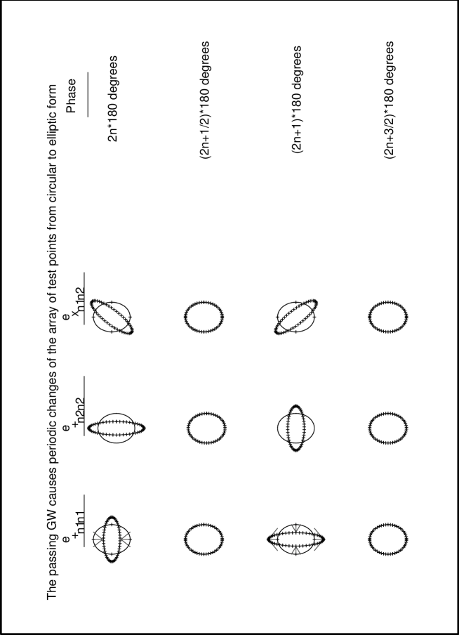
Figure 12: A schematic representation of the influence of a passing plane GW upon a circular (elliptic) array of test particles which periodically changes its form to elliptic (circular) array.

Substituting from Eq ($B_{11}$) into Eq ($B_{6}$) one obtains the components along ${\bf n}_{1}$ and ${\bf n}_{2}$ of the new location of the TP ${\cal B}$ as calculated in the proper reference frame of ${\cal A}$. That is, for $j={\bf n}_{1}$ one obtains [30]

$$x^{{\hat{\bf n_{1}}}}_{{\cal B}}=\Biggl{\{}x_{{\cal B}(0)}^{{\hat{\bf n_{1}}}}+\frac{1}{2}\biggl{(}A_{+}{\bf e}_{+_{\hat{{\bf n}}_{1}\hat{{\bf n}}_{1}}}x_{{\cal B}(0)}^{{\hat{\bf n_{1}}}}+A_{\times}{\bf e}_{\times_{\hat{{\bf n}}_{1}\hat{{\bf n}}_{2}}}x_{{\cal B}(0)}^{{\hat{\bf n_{2}}}}\biggr{)}\cdot B_{12}$$ ()

$$\cdot\cos\biggl{(}k\biggl{(}x\cos(\alpha)+y\cos(\beta)+z\cos(\eta)\biggr{)}-ft\biggr{)}\Biggr{\}}_{at{\cal A}}$$

And for $j={\bf n}_{2}$ one obtains [30]

$$x^{{\hat{\bf n_{2}}}}_{{\cal B}}=\Biggl{\{}x_{{\cal B}(0)}^{{\hat{\bf n_{2}}}}+\frac{1}{2}\biggl{(}A_{\times}{\bf e}_{\times_{\hat{{\bf n}}_{2}\hat{{\bf n}}_{1}}}x_{{\cal B}(0)}^{{\hat{\bf n_{1}}}}+A_{+}{\bf e}_{+_{\hat{{\bf n}}_{2}\hat{{\bf n}}_{2}}}x_{{\cal B}(0)}^{{\hat{\bf n_{2}}}}\biggr{)}\cdot B_{13}$$ ()

$$\cdot\cos\biggl{(}k\Bigl{(}x\cos(\alpha)+y\cos(\beta)+z\cos(\eta)\Bigr{)}-ft\biggr{)}\Biggr{\}}_{at{\cal A}}$$

B.2 The nonfringed trapped surface resulting from plane GW’s

As shown in [30] the comparison between the electromagnetic (EM) theory and the linearized general relativity enables one to use theoretical methods similar to those used in the EM theory for assuming interference and holographic properties for GW’s also. Similar comparison between these same theories has led to the concept of extrinsic time [39]. Thus, one may imagine [30] a subject ($S$) and reference ($R$) GW’s which constructively interfere and give rise to a spacetime holographic image [30, 31] which corresponds to the EM holographs [40] resulting from the interference of the $S$ and $R$ EM waves [40]. This line of reasoning was followed in [30, 31] and we introduce here some results obtained there. We note that for gravitational constructive interference the $S$ and $R$ GW’s, as for their EM analogues, should be similar and in phase with each other (see discussion in [30, 31]). Thus, the former expressions ($B_{9}$)-($B_{11}$) for the GW may be related not only to either $S$ or $R$ but also, in case of constructive interference, to the combined GW [30, 31] obtained from such an interference. The intensity, exposure and transmittance of this combined GW were calculated [31] in analogy with the corresponding EM quantities. It has also been shown in [30] that the holographic images resulting from this combined GW correspond to the trapped surfaces [18, 24, 25, 26] formed from such wave. Thus, since we discuss here these trapped surfaces we consider the former expressions ($B_{9}$)-($B_{11}$) and the following ones as referring to the combined GW obtained from the constructive interference of the $S$ and $R$ GW’s. We note that it has been shown [27, 28] that the collision of two plane GW’s results in a great strengthening (corresponds to constructive interference) of the resulting GW which forms, as is the case for strong GW’s [14, 24, 26, 21], a singularity [27, 28].

Now, since the trapped surfaces are embedded in the Euclidean space [14, 18, 24] one have first to convert [30] the tensor metric components (see Eqs ($B_{9}$)-($B_{10}$)) $h^{TT}_{\hat{{\bf n}}_{1}\hat{{\bf n}}_{1}}=-h^{TT}_{\hat{{\bf n}}_{2}\hat{{\bf n}}_{2}}$, $h^{TT}_{\hat{{\bf n}}_{1}\hat{{\bf n}}_{2}}=h^{TT}_{\hat{{\bf n}}_{2}\hat{{\bf n}}_{1}}$ from the ${\hat{\bf n}},\ {\hat{\bf n}}_{1},\ {\hat{\bf n}}_{2}$ system, into the ${\hat{\bf x}},\ {\hat{\bf y}},\ {\hat{\bf z}}$ Euclidean system. Thus, substituting [30] ${\hat{\bf n}}={\hat{\bf z}},\ {\hat{\bf n}}_{1}={\hat{\bf x}},\ {\hat{\bf n}}_{2}={\hat{\bf y}}$ one may write the Euclidean metric components as [30]

$$h^{TT}_{{\hat{\bf x}}{\hat{\bf x}}}=\Re\biggl{(}A_{+}{\bf e}_{+_{{\hat{\bf x}}{\hat{\bf x}}}}e^{-ift}e^{ik{\bf r}\hat{{\bf z}}}\biggr{)}=A_{+}{\bf e}_{+_{{\hat{\bf x}}{\hat{\bf x}}}}\cdot\cos(kz-ft)=$$

$$= -h^{TT}_{{\hat{\bf y}}{\hat{\bf y}}}=-\Re\biggl{(}A_{+}{\bf e}_{+_{{\hat{\bf y}}{\hat{\bf y}}}}e^{-ift}e^{ik{\bf r}\hat{{\bf z}}}\biggr{)}=-A_{+}{\bf e}_{+_{{\hat{\bf y}}{\hat{\bf y}}}}\cdot\cos(kz-ft) B_{14}$$ ()

$$h^{TT}_{{\hat{\bf x}}{\hat{\bf y}}}=\Re\biggl{(}A_{\times}{\bf e}_{\times_{{\hat{\bf x}}{\hat{\bf y}}}}e^{-ift}e^{ik{\bf r}\hat{{\bf z}}}\biggr{)}=A_{\times}{\bf e}_{\times_{{\hat{\bf x}}{\hat{\bf y}}}}\cdot\cos(kz-ft)=$$

$$= h^{TT}_{{\hat{\bf y}}{\hat{\bf x}}}=\Re\biggl{(}A_{\times}{\bf e}_{\times_{{\hat{\bf y}}{\hat{\bf x}}}}e^{-ift}e^{ik{\bf r}\hat{{\bf z}}}\biggr{)}=A_{\times}{\bf e}_{\times_{{\hat{\bf y}}{\hat{\bf x}}}}\cdot\cos(kz-ft),$$

where ${\bf r}=x{\hat{\bf x}}+y{\hat{\bf y}}+z{\hat{\bf z}}$ and ${\bf e}_{+_{{\hat{\bf x}}{\hat{\bf x}}}},\ {\bf e}_{+_{{\hat{\bf y}}{\hat{\bf y}}}},\ {\bf e}_{\times_{{\hat{\bf x}}{\hat{\bf y}}}}$ are the Euclidean unit linear-polarization tensors obtained [30] by substituting in Eqs ($B_{7}$)-($B_{8}$) ${\hat{\bf n}}={\hat{\bf z}},\ {\hat{\bf n}}_{1}={\hat{\bf x}},\ {\hat{\bf n}}_{2}={\hat{\bf y}}$. Thus, one may write the metrics from Eq ($B_{2}$) in the TT gauge as [30]

$$(ds^{TT})_{({\hat{\bf x}},{\hat{\bf y}},{\hat{\bf z}})}^{2}=h^{TT}_{{\hat{\bf x}}{\hat{\bf x}}}dx^{2}+h^{TT}_{{\hat{\bf y}}{\hat{\bf y}}}dy^{2}+2h^{TT}_{{\hat{\bf x}}{\hat{\bf y}}}dxdy=A_{+}{\bf e}_{+_{{\hat{\bf x}}{\hat{\bf x}}}}\cdot\cos(kz-ft)dx^{2}+$$

$$+ A_{+}{\bf e}_{+_{{\hat{\bf y}{\hat{\bf y}}}}}\cdot\cos(kz-ft)dy^{2}+2A_{\times}{\bf e}_{\times_{{\hat{\bf x}}{\hat{\bf y}}}}\cdot\cos(kz-ft)dxdy= B_{15}$$ ()

$$= A_{+}{\bf e}_{+_{{\hat{\bf x}}{\hat{\bf x}}}}\cdot\cos(kz-ft)(dx^{2}-dy^{2})+2A_{\times}{\bf e}_{\times_{{\hat{\bf x}{\hat{\bf y}}}}}\cdot\cos(kz-ft)dxdy,$$

where we use [30] ${\bf e}_{+_{{\hat{\bf x}}{\hat{\bf x}}}}=-{\bf e}_{+_{{\hat{\bf y}}{\hat{\bf y}}}}$ (see Eq ($B_{7}$)). For calculating the nonfringed embedded surface one have to convert [30] the last metric from the $({\hat{\bf x}},\ {\hat{\bf y}},\ {\hat{\bf z}})$ system to the cylindrical one $({\hat{\bf\rho}},\ {\hat{\bf\phi}},\ {\hat{\bf z}})$ where $x=\rho\cos(\phi),\ y=\rho\sin(\phi),\ z=z$. Thus, using the trigonometric relations $(\cos^{2}(\phi)-\sin^{2}(\phi))=\cos(2\phi)$, $2\sin(\phi)\cos(\phi)=\sin(2\phi)$ and transforming the unit polarization tensors ${\bf e}_{+_{{\hat{\bf x}}{\hat{\bf x}}}},\ {\bf e}_{+_{{\hat{\bf xy}}}}$ to the corresponding cylindrical ones ${\bf e}_{+_{{\hat{\bf\rho}}{\hat{\bf\rho}}}},\ {\bf e}_{+_{{\hat{\bf\rho}}{\hat{\bf\phi}}}}$ one obtains [30]

$$( ds^{TT})_{({\hat{\bf\rho}},{\hat{\bf\phi}},{\hat{\bf z}})}^{2}=h^{TT}_{{\hat{\bf\rho}}{\hat{\bf\rho}}}d\rho^{2}+h^{TT}_{{\hat{\bf\phi}}{\hat{\bf\phi}}}d\phi^{2}+h^{TT}_{{\hat{\bf\rho}}{\hat{\bf\phi}}}d\rho d\phi=$$

$$= A_{+}{\bf e}_{+_{{\hat{\bf\rho}}{\hat{\bf\rho}}}}\cdot\cos(kz-ft)\bigg{(}\cos(2\phi)(d\rho^{2}-\rho^{2}d\phi^{2})-2\rho\sin(2\phi)d\rho d\phi\biggr{)} B_{16}$$ ()

$$+ A_{\times}{\bf e}_{\times_{{\hat{\bf\rho}}{\hat{\bf\phi}}}}\cdot\cos(kz-ft)\biggl{(}\sin(2\phi)(d\rho^{2}-\rho^{2}d\phi^{2})+2\rho\cos(2\phi)d\rho d\phi\biggr{)},$$

where the unit polarization tensor components ${\bf e}_{+_{{\hat{\bf\rho}}{\hat{\bf\rho}}}},\ {\bf e}_{+_{{\hat{\bf\rho}}{\hat{\bf\phi}}}}$ are given by [30]

$${\bf e}_{+_{{\hat{\bf\rho}}{\hat{\bf\rho}}}}=\cos(2\phi)\biggl{(}{\bf e}_{\hat{\bf\rho}}\otimes{\bf e}_{\hat{\bf\rho}}-{\bf e}_{\hat{\bf\phi}}\otimes{\bf e}_{\hat{\bf\phi}}\biggr{)}-\sin(2\phi)\biggl{(}{\bf e}_{\hat{\bf\rho}}\otimes{\bf e}_{\hat{\bf\phi}}+{\bf e}_{\hat{\bf\phi}}\otimes{\bf e}_{\hat{\bf\rho}}\biggr{)} B_{17}$$ ()

$${\bf e}_{\times_{{\hat{\bf\rho}}{\hat{\bf\phi}}}}=\sin(2\phi)\biggl{(}{\bf e}_{\hat{\bf\rho}}\otimes{\bf e}_{\hat{\bf\rho}}-{\bf e}_{\hat{\bf\phi}}\otimes{\bf e}_{\hat{\bf\phi}}\biggr{)}+\cos(2\phi)\biggl{(}{\bf e}_{\hat{\bf\rho}}\otimes{\bf e}_{\hat{\bf\phi}}+{\bf e}_{\hat{\bf\phi}}\otimes{\bf e}_{\hat{\bf\rho}}\biggr{)}$$

The last tensor components are obtained by using: (1) ${\bf e}_{+_{{\hat{\bf x}}{\hat{\bf x}}}}={\bf e}_{\hat{\bf x}}\otimes{\bf e}_{\hat{\bf x}}-{\bf e}_{\hat{\bf y}}\otimes{\bf e}_{\hat{\bf y}}=-{\bf e}_{+_{{\hat{\bf y}}{\hat{\bf y}}}},\ \ {\bf e}_{\times_{{\hat{\bf x}}{\hat{\bf y}}}}={\bf e}_{\hat{\bf x}}\otimes{\bf e}_{\hat{\bf y}}+{\bf e}_{\hat{\bf y}}\otimes{\bf e}_{\hat{\bf x}}={\bf e}_{\times_{\hat{\bf y}{\hat{\bf x}}}}$ which are obtained from Eqs ($B_{7}$)-($B_{8}$) by substituting [30] ${\hat{\bf n}}={\hat{\bf z}},\ {\hat{\bf n}}_{1}={\hat{\bf x}},\ {\hat{\bf n}}_{2}={\hat{\bf y}}$, (2) ${\bf e}_{\hat{\bf x}}=\cos(\phi){\bf e}_{\hat{\bf\rho}}-\sin(\phi){\bf e}_{\hat{\phi}},\ \ {\bf e}_{\hat{\bf y}}=\sin(\phi){\bf e}_{\hat{\bf\rho}}+\cos(\phi){\bf e}_{\hat{\phi}},\ \ {\bf e}_{\hat{\bf z}}={\bf e}_{\hat{\bf z}}$ [37] and (3) $(\cos^{2}(\phi)-\sin^{2}(\phi))=\cos(2\phi)$, $2\cos(\phi)\sin(\phi)=\sin(2\phi)$. As mentioned after Eq (20), ${\bf e}_{+_{{\hat{\bf\rho}}{\hat{\bf\rho}}}}$, ${\bf e}_{\times_{{\hat{\bf\rho}}{\hat{\bf\phi}}}}$ as well as ${\bf e}_{\hat{\bf\rho}}\otimes{\bf e}_{\hat{\bf\rho}}$, ${\bf e}_{\hat{\bf\rho}}\otimes{\bf e}_{\hat{\bf\phi}}$ and ${\bf e}_{\hat{\bf\phi}}\otimes{\bf e}_{\hat{\bf\phi}}$ are tensor components in the $\rho\rho$, $\rho\phi$ and $\phi\phi$ directions and so, of course, they are not tensors proper. This enables one to perform some mathematical operations on these components such as comparing them to functions or taking their square roots as done, for example, in Eqs (20)-(24).

Assuming [30], as in [17, 20, 18], a non-rotating system so that $h^{TT}_{{\hat{\bf\rho}}{\hat{\bf\phi}}}$ is identically zero one may write Eq ($B_{16}$) as [30]

$$( ds^{TT})_{({\hat{\bf\rho}},{\hat{\bf\phi}},{\hat{\bf z}})}^{2}=h^{TT}_{{\hat{\bf\rho}}{\hat{\bf\rho}}}d^{2}\rho+h^{TT}_{{\hat{\bf\phi}}{\hat{\bf\phi}}}d^{2}\phi= B_{18}$$ ()

$$= \cos(kz-ft)\biggl{(}A_{+}{\bf e}_{+_{{\hat{\bf\rho}}{\hat{\bf\rho}}}}\cos(2\phi)+A_{\times}{\bf e}_{\times_{{\hat{\bf\rho}}{\hat{\bf\phi}}}}\sin(2\phi)\biggr{)}\biggl{(}(d\rho^{2}-\rho^{2}d\phi^{2})\biggr{)}=$$

$$= \cos(kz-ft)\biggl{[}\frac{\sin(4\phi)}{2}(A_{\times}-A_{+})\left({\bf e}_{\hat{\bf\rho}}\otimes{\bf e}_{\hat{\bf\phi}}+{\bf e}_{\hat{\bf\phi}}\otimes{\bf e}_{\hat{\bf\rho}}\right)+$$

$$+ \left(A_{+}\cos^{2}(2\phi)+A_{\times}\sin^{2}(2\phi)\right)\biggl{(}{\bf e}_{\hat{\bf\rho}}\otimes{\bf e}_{\hat{\bf\rho}}-{\bf e}_{\hat{\bf\phi}}\otimes{\bf e}_{\hat{\bf\phi}}\biggr{)}\biggr{]}\left(d^{2}\rho-\rho^{2}d\phi^{2}\right)$$

Note that when $A_{\times}=A_{+}$ the expression $\biggl{(}A_{+}{\bf e}_{+_{{\hat{\bf\rho}}{\hat{\bf\rho}}}}\cos(2\phi)+A_{\times}{\bf e}_{\times_{{\hat{\bf\rho}}{\hat{\bf\phi}}}}\sin(2\phi)\biggr{)}$ is considerably simplified and reduces [30] to

$$\biggl{(}A_{+}{\bf e}_{+_{{\hat{\bf\rho}}{\hat{\bf\rho}}}}\cos(2\phi)+A_{\times}{\bf e}_{\times_{{\hat{\bf\rho}}{\hat{\bf\phi}}}}\sin(2\phi)\biggr{)}=A_{+}\biggl{(}{\bf e}_{\hat{\bf\rho}}\otimes{\bf e}_{\hat{\bf\rho}}-{\bf e}_{\hat{\bf\phi}}\otimes{\bf e}_{\hat{\bf\phi}}\biggr{)}$$

We, now, find the relevant nonfringed embedded surface and assume [30], as done for the nonfringed trapped surfaces resulting from the Brill’s GW [18] (see Appendix A here), that its metric is that of a surface of rotation $z(x,y)$ related to Euclidean space as

$$x^{P}=f^{P}(\rho)\cos(\phi),\ \ y^{P}=f^{P}(\rho)\sin(\phi),\ \ z^{P}=h^{P}(\rho), B_{19}$$ ()

where the superscript $P$ denotes that we consider plane GW’s. Thus, using Eqs $B_{18}$ one may write the metric of the relevant holographic image (trapped surface) as [30] (compare with Eq ($A_{12}$) in Appendix A for the Brill case),

$$d s^{2}=dx^{2}+dy^{2}+dz^{2}=\biggl{(}(f^{P})_{\rho}^{2}(\rho)+(h^{P})_{\rho}^{2}(\rho)\biggr{)}d\rho^{2}+(f^{P})^{2}(\rho)d\phi^{2}= B_{20}$$ ()

$$= h^{TT}_{{\hat{\bf\rho}}{\hat{\bf\rho}}}d^{2}\rho+h^{TT}_{{\hat{\bf\phi}}{\hat{\bf\phi}}}d^{2}\phi=\cos(kz-ft)\biggl{(}A_{+}{\bf e}_{+_{{\hat{\bf\rho}}{\hat{\bf\rho}}}}\cos(2\phi)+A_{\times}{\bf e}_{\times_{{\hat{\bf\rho}}{\hat{\bf\phi}}}}\sin(2\phi)\biggr{)}\cdot$$

$$\cdot \biggl{(}d\rho^{2}-\rho^{2}d\phi^{2}\biggr{)}=\cos(kz-ft)\biggl{[}\frac{\sin(4\phi)}{2}(A_{\times}-A_{+})\left({\bf e}_{\hat{\bf\rho}}\otimes{\bf e}_{\hat{\bf\phi}}+{\bf e}_{\hat{\bf\phi}}\otimes{\bf e}_{\hat{\bf\rho}}\right)+$$

$$+ \left(A_{+}\cos^{2}(2\phi)+A_{\times}\sin^{2}(2\phi)\right)\biggl{(}{\bf e}_{\hat{\bf\rho}}\otimes{\bf e}_{\hat{\bf\rho}}-{\bf e}_{\hat{\bf\phi}}\otimes{\bf e}_{\hat{\bf\phi}}\biggr{)}\biggr{]}\left(d^{2}\rho-\rho^{2}d\phi^{2}\right)$$

where Eq ($B_{17}$) was used and by $f^{P}_{\rho}(\rho),\ h^{P}_{\rho}(\rho)$ we denote the first derivatives of $f^{P}(\rho),\ h^{P}(\rho)$ with respect to $\rho$. Using Eq ($B_{20}$) one may determine [30] the quantities $f^{P}(\rho)$, $f^{P}_{\rho}(\rho)$ and $h^{P}(\rho)$ which defines the intrinsic geometry of the nonfringed trapped surface (gravitational holograph)

$$f^{P}(\rho)=\rho\biggl{[}\cos(kz-ft)\biggl{\{}\frac{\sin(4\phi)}{2}(A_{+}-A_{\times})\left({\bf e}_{\hat{\bf\rho}}\otimes{\bf e}_{\hat{\bf\phi}}+{\bf e}_{\hat{\bf\phi}}\otimes{\bf e}_{\hat{\bf\rho}}\right)+$$

$$+ \left(A_{+}\cos^{2}(2\phi)+A_{\times}\sin^{2}(2\phi)\right)\biggl{(}{\bf e}_{\hat{\bf\phi}}\otimes{\bf e}_{\hat{\bf\phi}}-{\bf e}_{\hat{\bf\rho}}\otimes{\bf e}_{\hat{\bf\rho}}\biggr{)}\biggr{\}}\biggr{]}^{\frac{1}{2}}$$

$$f^{P}_{\rho}(\rho)=\biggl{[}\cos(kz-ft)\biggl{\{}\frac{\sin(4\phi)}{2}(A_{+}-A_{\times})\left({\bf e}_{\hat{\bf\rho}}\otimes{\bf e}_{\hat{\bf\phi}}+{\bf e}_{\hat{\bf\phi}}\otimes{\bf e}_{\hat{\bf\rho}}\right)+$$

$$+ \left(A_{+}\cos^{2}(2\phi)+A_{\times}\sin^{2}(2\phi)\right)\biggl{(}{\bf e}_{\hat{\bf\phi}}\otimes{\bf e}_{\hat{\bf\phi}}-{\bf e}_{\hat{\bf\rho}}\otimes{\bf e}_{\hat{\bf\rho}}\biggr{)}\biggl{\}}\biggr{]}^{\frac{1}{2}} B_{21}$$ ()

$$h^{P}(\rho)=\int d\rho\biggl{[}\cos(kz-ft)\biggl{\{}\frac{\sin(4\phi)}{2}(A_{\times}-A_{+})\left({\bf e}_{\hat{\bf\rho}}\otimes{\bf e}_{\hat{\bf\phi}}+{\bf e}_{\hat{\bf\phi}}\otimes{\bf e}_{\hat{\bf\rho}}\right)+$$

$$+ \left(A_{+}\cos^{2}(2\phi)+A_{\times}\sin^{2}(2\phi)\right)\biggl{(}{\bf e}_{\hat{\bf\rho}}\otimes{\bf e}_{\hat{\bf\rho}}-{\bf e}_{\hat{\bf\phi}}\otimes{\bf e}_{\hat{\bf\phi}}\biggr{)}\biggr{\}}-(f^{P})_{\rho}^{2}(\rho)\biggr{]}^{\frac{1}{2}}$$

References

- [1]
- [2] M. Shamos, “Great experiments in physics”, Dover, New York (1987)
- [3] Thomas Young, “Experimental demonstrations of the general law of the interference of light”, Phil. Trans. Roy. Soc. London, 94 (1804)
- [4] A. A. Michelson and E. W. Morley, Am. J. Sci, 134, 333 (1887)
- [5] P. G. Bergmann, "Introduction to the theory of relativity", Dover (1976)
- [6] E. Merzbacher, “Quantum Mechanics", Second edition, by John Wiley, New York, 1961; Claude Cohen Tannoudji, Bernard Diu and Franck Laloe, “Quantum Mechanics”, John Wiley, (1977)
- [7] L. I. Schiff, “Quantum Mechanics”, 3-rd Edition, McGraw-Hill (1968)
- [8] Francis. A. Jenkins and Harvey. E. White, Fundamentals of Optics, 4-th Edition, McGraw-Hill (1976)
- [9] J. A. Wheeler and W. H. Zurek, ed, “Quantum Theory and measurement", Princeton Univ Press (1983)
- [10] A. G. Zajonc, “Quantum eraser”, Nature 353, 507 (1991); P. G. Kwiat, A. M. Steinberg and R. Y. Chiao, “Three proposed "quantum erasers"”, Phys. Rev A 49, 61 (1994); T. J. Herzog, P. G. Kwiat, H. Weinfurter and A. Zeilinger, “ Complementarity and the quantum eraser”, Phys. Rev. Lett 75, 3034 (1995); T. B. Pittman, D. V. Strekalov, A. Migdall, M. H. Rubin, A. V. Sergienko and H. H. Shih, “ Can two-photon interference be considered the interference of two photons ?”, Phys. Rev. Lett 77, 1917 (1996): Summary of the experiments decribed in these references is available at: http://www.bottomlayer.com/bottom/basic delayed choice.htm
- [11] D. Finkelstein, Action physics, Inter. J. Theor. Phys, 38, 1, 447 (1999)
- [12] Yoon-Ho Kim, R. Yu, S. P. Kulik, Y. H. Shih and M. O. Scully, “ A delayed choice quantum eraser”, Phys. Rev. Lett 84 1-5 (2000). Commentary and summary of this experiment is available at: http://www.bottomlayer.com/bottom/kim-scully/kim-scully-web.htm
- [13] The kind of digital camera used was HP Photosmart M22 and the photographs taken were in JPEG format which were converted to the PS one.
- [14] C. W. Misner, K. S. Thorne and J. A. Wheeler, "Gravitation", Freeman, San Francisco (1973)
- [15] J. B. Hartle, “Gravity: An introduction to Einstein’s general relativity”, Addison-Wesley, San Fracisco (2003)
- [16] K. S. Thorne, “Multipole expansions of gravitational radiation”, Rev. Mod. Phys 52, 299 (1980); K. S. Thorne, “Gravitational wave research: Current status and future prospect”, Rev. Mod. Phys 52, 285 (1980)
- [17] D. R. Brill, “On the positive definite mass of the Bondi-Weber-Wheeler time-symmetric gravitational waves”, Ann. Phys, 7, 466 (1959); D. R. Brill, Suppl. Nuovo. Cimento, 2, 1-56 (1964); D. R. Brill and J. B. Hartle, “Method of the self-consistent field in General Relativity and its application to the gravitational geon”, Phys. Rev B, 135, 271 (1964); N. O. Murchadha, “Brill waves”, gr-qc/9302023 (1993)
- [18] K. Eppley, “Evolution of time-symmetric gravitational waves: Initial data and apparent horizons”, Phys. Rev D, 16, 1609 (1977);
- [19] S. M. Miyama, "Time evolution of pure gravitational wave" Prog. Theor. Phys, 65, 894 (1981); T. Nakamura, “General solutions of the linearized Einstein equations and initial data for three dimensional evolution of pure gravitational waves”, Prog. Theor. Phys, 72, 746 (1984)
- [20] A. P. Gentle, D. E. Holz and W. A. Miller, “Apparent horizons in simplical Brill wave initial data", Class. Quant. Grav, 16, 1979-1985 (1999); A. P. Gentle, "Simplical Brill wave initial data", Class. Quant. Grav, 16, 1987-2003 (1999)
- [21] M. Alcubierre, G. Allen, B. Brugmann, G. Lanfermann, E. Seidel, W. M. Suen and M. Tobias, “Gravitational collapse of gravitational waves in 3-D numerical relativity”, Phys. Rev D, 61, 041501 (2000);
- [22] D. Finkelstein and E. Rodriguez, “Relativity of topology and dynamics”, Inter, J, Theor, Phys, 23, 1065-1098 (1984)
- [23] R. D. Sorkin, “Topology change and monopole creation”, Phys. Rev D, 33, 978 (1986)
- [24] D. Brill and R. W. Lindquist, “Interaction energy in Geometrodynamics”, Phys. Rev, 131, 471-476 (1963);
- [25] R. Beig and N. O. Murchadha, “ Trapped surfaces due to concentration of gravitational radiation”, Phys. Rev Lett, 66, 2421 (1991)
- [26] A. M. Abrahams and C. R. Evans, “Trapping a geon: Black hole formation by an imploding gravitational wave”, Phys. Rev D, 46, R4117 (1992)
- [27] F. J. Tipler, “ Singularities from colliding plane gravitational waves ”, Phys. Rev D, 22, 2929 (1980)
- [28] U. Urtsever, “Singularities in the collisions of almost-plane gravitational waves”, Phys. Rev D, 38, 1731 (1988); “Colliding almost-plane gravitational waves: Colliding plane waves and general properties of almost-plane wave spacetimes”, Phys. Rev D, 37, 2803 (1988)
- [29] R. Arnowitt, S. Desser and C. W. Misner, “The dynamics of General Relativity” In “Gravitation: An Introduction to current research”, ed. L. Witten, Wiley, New-York (1962)
- [30] D. Bar, “Gravitational holography and trapped surfaces”, Inter. J. Theor. Phys, 46, 664-687 (2007).
- [31] D. Bar, “Gravitational wave holography”, Inter. J. Theor. Phys, 46, 503-517 (2007).
- [32] N. Bohr, “ The quantum postulate and the recent development of atomic theory”, Nature 121, 580 (1928); “Can Quantum Mechanical description of physical reality be considered complete ?”, Phys. Rev 48, 696 (1935); "Atomic theory and description of nature" , Cambridge, London (1934)
- [33] S. W. Hawking and G. F. R. Ellis, “The large scale structure of spacetime”, Cambridge, London (1973)
- [34] K. Kuchar, “Canonical quantization of cylindrical gravitational waves”, Phys. Rev D , 4, 955 (1971)
- [35] M. R. Spiegel, “Fourier analysis”, Schaum’s Outline Series, McGraw-hill, New-York (1974).
- [36] L. A. Pipes, “Applied mathematics for engineers and physicists”, Second edition, McGraw-Hill, New-York (1958)
- [37] M. R. Spiegel, “Vector analysis”, Schaum’s Outline Series, McGraw-hill, New-York (1959).
- [38] J. L. Synge and A. Schild, "Tensor Calculus", Dover (1978)
- [39] K. Kuchar, “Ground state functional of the linearized gravitational field”, J. Math. Phys, 11, 3322 (1970)
- [40] R. J. Collier, C. B. Burckhardt and L. H. Lin, “Optical Holography”, Academic Press (1971)