Density Perturbations for Running Cosmological Constant

Abstract:

The dynamics of density and metric perturbations is investigated for the previously developed model where the decay of the vacuum energy into matter (or vice versa) is due to the renormalization group (RG) running of the cosmological constant (CC) term. The evolution of the CC depends on the single parameter $\nu$, which characterizes the running of the CC produced by the quantum effects of matter fields of the unknown high energy theory below the Planck scale. The sign of $\nu$ indicates whether bosons or fermions dominate in the running. The spectrum of perturbations is computed assuming an adiabatic regime and an isotropic stress tensor. Moreover, the perturbations of the CC term are generated from the simplest covariant form suggested by the RG model under consideration. The corresponding numerical analysis shows that for $\nu>0$ there is a depletion of the matter power spectrum at low scales (large wave numbers) as compared to the standard $\Lambda$CDM model, whereas for $\nu<0$ there is an excess of power at low scales. We find that the LSS data rule out the range $\left|\nu\right|>10^{-4}$ while the values $\left|\nu\right|\leq 10^{-6}$ look perfectly acceptable. For $\nu<0$ the excess of power at low scales grows rapidly and the bound is more severe. From the particle physics viewpoint, the values  $|\nu|\simeq 10^{-6}$ correspond to the “desert” in the mass spectrum above the GUT scale $M_{X}\sim 10^{16}\,GeV$. Our results are consistent with those obtained in other dynamical models admitting an interaction between dark matter and dark energy. We find that the matter power spectrum analysis is a highly efficient method to discover a possible scale dependence of the vacuum energy.

1 Introduction

The analysis of cosmic perturbations [1, 2, 3] represents one of the main tests for the candidate cosmological models and especially for the models of a time-dependent Dark Energy (DE). The recent data on the accelerated expansion of the Universe from the high redshift Type Ia supernovae [4], combined with the measurements of the CMB anisotropies [5, 6, 7] and LSS [8, 9] indicate that the DE is responsible for most of the energy balance in the present Universe. The natural candidate to be the DE is the cosmological constant, mainly if we take into account that from the quantum field theory (QFT) point of view the zero value of the CC would be extremely unnatural [10, 11, 12]. The solution of the standard CC problems, such as the origin of the fine-tuning between vacuum and induced counterparts and the problem of coincidence, is not known. Historically the first attempts to solve some of these problems went along the lines of dynamical adjustments mechanisms [13]. Nowadays the discussion is approached from many different perspectives and has generated an extensive literature, see e.g.  [14, 15] and references therein. One of the most interesting aspects of these discussions is the possibility to have a slowly varying DE density of the Universe [16]. This option cannot be ruled out by the analysis of the present data [17, 18]. In case that the new generation of cosmic observational experiments will indeed detect a variable DE, the natural question to ask is: would this fact really mean the manifestation of a qualitatively new physical reality such as quintessence [19], Chaplygin gas [20], extra dimensions [21] or of low-energy quantum gravity [22, 23, 24, 25]? Let us emphasize here that one cannot honestly address this question without also exploring the possibility of a time-variable CC whose running is due to known physical effects, that is, due to the quantum effects of matter fields on a curved classical background [26].

The most natural manner to investigate the possible running of the CC produced by the quantum effects of matter fields is the renormalization group (RG) in curved space-time [27, 11, 12]. Unfortunately, the existing calculational methods are not sufficient for performing a complete theoretical investigation of this problem [28]. At the same time, the phenomenological proposal [11, 12, 29, 30] shows that a positive result can not be ruled out. The hypothesis of a standard quadratic form of decoupling for the quantum effects of matter fields at low energies [11, 31] leads to consistent cosmological models of a running CC with potentially observable consequences [32, 33, 34, 35, 36]. Among the many possibilities one can distinguish essentially two different models of running CC in QFT in curved space-time . The first one [29, 30, 32] admits that there is energy exchange between matter and vacuum sectors of the theory . This leads to the vacuum energy density function $\rho_{\Lambda}=\rho_{\Lambda}(H)$ associated to the cosmological term, $\Lambda$, while the Newton constant $G$ remains invariable . The second model does not admit a matter-vacuum energy exchange, but has both parameters scale-dependent $G=G(H)$ and $\rho_{\Lambda}=\rho_{\Lambda}(H)$ [34]. In the present work we shall concentrate on the analysis of the perturbations for the first model only, and postpone the investigation of the second model for another publication. Let us remark that the analysis of cosmic perturbations in the first model has already been addressed in [40] using an indirect procedure based on bounding the amplification of the density matter spectrum in the recombination era caused by vacuum decay into CDM. This amplification is necessary to compensate for the dilution of the $\delta\rho_{m}/\rho_{m}$ matter spectrum at low redshifts resulting from the enhanced matter-radiation density $\rho_{m}$ – associated to the decay of the vacuum into CDM. A qualitatively similar analysis has been performed in [41], and also in [42] using the so-called CMB shift parameter [6]. It is worth noticing that the upper bounds for the running obtained in all these references disagree between themselves, in some cases at the level of several orders of magnitude. This severe divergence illustrates the importance and necessity of performing a direct calculation of the perturbations, which we undertake here thoroughly. For example, the estimate used in [40] was derived from the phenomenological study presented in Ref. [43], where the matter power spectrum of density fluctuations measured by the 2dF Galaxy Redshift Survey (2dFGRS) was compared with the corresponding matter power spectrum derived from the measurements of the CMB anisotropies. The comparison served to place a bound at the level of $10\%$ on the maximum possible difference between the two derivations of the matter power spectrum [43]. By requiring that the amplification of the density fluctuations of the RG model at the recombination era do not surpass this bound the authors of [40] were able to obtain a corresponding bound on the the RG parameter of [29], specifically $\nu<10^{-3}$. Of course this bound is only approximate as it does not come from a direct calculation of the density perturbations in the RG model. Notwithstanding, as we shall see in what follows, there is a qualitative agreement between these results and the ones obtained in the direct calculation that we present here. In both cases the RG models with Planck-scale mass particles are not favored and one is led to conclude that a significant energy gap (or “desert”) below the Planck scale, $M_{P}$, is necessary to avoid contradictions between the calculated spectrum of the density perturbations and the observational data. The favored mass scale turns out to be three orders of magnitude below $M_{P}$, and can be identified with the typical GUT scale $M_{X}\sim 10^{16}\,GeV$. In this paper we will provide a rigorous quantitative derivation of this result. Let us also remark that the analysis of perturbations presented here is not covered by the many works in the literature dealing with perturbations in a Universe with dynamical dark energy – see e.g.  [15] and references therein. In fact, the nature of the DE under consideration is not directly related to the properties of dynamical scalar field(s), but to the QFT running of the cosmological constant. Therefore, our approach is qualitatively new and has not been dealt with in the literature before. It constitutes, to our knowledge, the first computation of density perturbations in the presence of a running cosmological term. This is important in order to assess the impact on structure formation from a possible scale dependence of the vacuum energy.
The paper is organized as follows. In the next section we summarize the necessary information about the variable CC model under discussion. The reader may consult the papers [11, 29, 32, 33] for further technical details and extensive discussions. In section 3 we derive the equations for the perturbations. Section 4 is devoted to the numerical solution of these equations and to their comparison with the 2dFGRS [8]. Finally, in the last section we draw our conclusions.

2 The background cosmological solution in the running CC model

In the framework under consideration[11, 29], with renormalization group corrected CC and energy exchange between vacuum and matter sectors, the cosmological evolution is governed by the following three ingredients:  $(i)$ Friedmann equation,

$$H^{2}(z)=\frac{8\,\pi\,G}{3}\,\big{[}\rho_{m}(z)+\rho_{\Lambda}(z)\big{]}\,+\,H_{0}^{2}\Omega_{k}^{0}\,(1+z)^{2}\,,$$ (1)

where  $\rho_{m}(z)$  and  $\rho_{\Lambda}(z)$  are the densities of matter and vacuum energies taken as functions of the cosmological redshift, $z$, with  $H_{0}^{2}\,\Omega_{k}^{0}(1+z)^{2}=-k/a^{2}$;  $(ii)$ Conservation law (following from the Bianchi identity) which regulates the exchange of energy between matter and vacuum,

$$\frac{d\rho_{\Lambda}}{dz}+\frac{d\rho_{m}}{dz}\,=\,\frac{3\,\rho_{m}}{1+z}\,,$$ (2)

and  $(iii)$ the renormalization group equation for the CC density, assuming a soft form of decoupling for the cosmological constant [11, 29, 31]

$$\frac{d\rho_{\Lambda}}{d{\,\mbox{ln}\,H}}=\frac{1}{(4\pi)^{2}}\ \sigma\,H^{2}M^{2}\,.$$ (3)

In this equation, the effective mass $M$  represents an additive sum of the contributions of all virtual massive particles, and $\,\sigma=\pm 1$ depending on whether fermions or bosons dominate at the highest energies. It proves useful introducing the new (dimensionless) parameter

$$\nu\equiv\frac{\sigma}{12\,\pi}\,\frac{M^{2}}{M_{P}^{2}}\,.$$ (4)

The value of $\nu$ defines the strength of the quantum effects and has direct physical interpretation. For example, taking the “canonical” value $\nu=\nu_{0}\equiv 1/12\pi=0.026$ means that the effective cumulative mass $M$ of all virtual massive particles is equal to the Planck mass, whereas $|\nu|\sim 1$ means the existence of a particle with trans-planckian mass or of nearly Planck-mass particles with huge multiplicities. Taking $|\nu|\sim 10^{-6}$ means that the spectrum of particles is bounded from above at the (GUT) scale  $M_{X}\approx 10^{16}\,GeV\sim 10^{-3}M_{P}$. Much smaller values of  $|\nu|\ll 10^{-6}$  mean the existence of an extra unbroken symmetry between bosons and fermions (e.g. supersymmetry) at the GUT scale etc.

We already noticed that Eq. (2) implies the possibility of an energy transfer between vacuum and matter, which may be interpreted as a decay of the vacuum into matter or vice versa. While the decay of the vacuum energy into ordinary matter and radiation could be problematic for the observed CMB, the decay into CDM can be allowed [16, 46] provided the rate is sufficiently small. It is of course part of the present study to evaluate the possible size of this rate.

The complete analytic solution of the equations (1), (2), (3) can be found in [29, 32]. Here we present only those formulas which are relevant for the perturbations calculus. First of all, from (3) it follows that

$$\rho_{\Lambda}(z;\nu)\,=\,\rho_{\Lambda}^{0}+\frac{3\,\nu}{8\pi}\,M_{P}^{2}\,\left(H^{2}-H^{2}_{0}\right)\,.$$ (5)

Furthermore, we introduce notations for the pressure and density of the vacuum and matter components, such that the total values become (we assume pressureless matter at present)

$$\rho_{t}=\rho_{m}+\rho_{\Lambda}\,,\qquad P_{t}=P_{m}+P_{\Lambda}\,,\qquad\mbox{where}\qquad P_{\Lambda}=-\rho_{\Lambda}\,,\qquad P_{m}=0\,.$$ (6)

The quantities (6) determine the dynamical evolution law for the scale factor:

$${\dot{H}}+H^{2}=\frac{{\ddot{a}}}{a}=-\frac{4\pi G}{3}\,(\rho_{t}+3P_{t})=-\frac{4\pi G}{3}\,(\rho_{m}-2\rho_{\Lambda})\,.$$ (7)

What we shall need in what follows are the two ratios

$$f_{1} = f_{1}(z)\,\,=\,\,\frac{\rho_{m}}{\rho_{t}}=\frac{(1+z)(H^{2})^{\prime}-2H_{0}^{2}\,\Omega_{k}^{0}(1+z)^{2}}{3\left[H^{2}-H_{0}^{2}\,\Omega_{k}^{0}(1+z)^{2}\right]}\,,$$

$$f_{2} = f_{2}(z)\,\,=\,\,\frac{\rho_{\Lambda}}{\rho_{t}}=\frac{3H^{2}-(1+z)(H^{2})^{\prime}-H_{0}^{2}\,\Omega_{k}^{0}(1+z)^{2}}{3\left[H^{2}-H_{0}^{2}\,\Omega_{k}^{0}(1+z)^{2}\right]}\,,$$ (8)

where the prime indicates  $d/dz$. The expansion rate  $H(z)$ in this model is given as follows:

$$H^{2}(z;\nu)\,=\,H_{0}^{2}+\left(\Omega_{M}^{0}-\frac{2\nu\Omega_{k}^{0}}{1-3\,\nu}\right)\,\frac{H_{0}^{2}\,\left[(1+z)^{3-3\nu}-1\right]}{1-\nu}+\frac{\Omega_{k}^{0}H_{0}^{2}(z^{2}+2z)}{1-3\,\nu}\,.$$ (9)

In the last formula $\Omega_{M}^{0}=\Omega_{DM}^{0}+\Omega_{B}^{0}$ is the sum of the Dark Matter (DM) and baryonic matter densities (relative to the critical density) in the present-day Universe. Let us remark that the scale dependence of the vacuum energy (5) does not imply a change of the equation of state for the “cosmological constant fluid”. In this work we follow [29, 30, 32] and assume that  $p_{\Lambda}=-\rho_{\Lambda}$, even when quantum corrections are taken into account. It should be clear that this equation of state is valid irrespective of whether $\Lambda$ is constant or variable. A different issue is that the models with variable cosmological parameters (like the present one) can be interpreted in terms of an effective equation of state corresponding to a self-conserved dark energy, as it is usually assumed in e.g. scalar field models of the DE. The general framework for this effective EOS analysis has been developed in [35, 36], where a particular discussion of this issue for the present running CC model is also included.

3 Deriving the perturbations equations

In order to derive the equations for the density and metric perturbations we follow the standard formalism (see e.g. [1]-[3]). We will perform our calculation of density perturbations under the following two assumptions:

• The entropic perturbations are negligible;

• The full energy-momentum tensor is free of anisotropic stresses.

In the absence of more information we believe that these hypotheses are reasonable as they aim at the maximum simplicity in the presentation of our results. Notice that in a single fluid case, the pressureless fluid and the vacuum equation of state have zero anisotropic pressure [2]; if both fluids interact, as it happens in the present case, a contribution can appear, but we cannot model it without introducing further free parameters. Similarly, the contribution of entropic perturbations must be introduced phenomenologically, and this would lead to the appearance of more free parameters, thus masking any constraint we can obtain on the fundamental parameter $\nu$ of our RG framework. It should also be stressed that the same approximations are made in similar works in the literature, for example in reference [47] where the density perturbations in the alternative framework of interacting quintessence models are considered and a corresponding bound on the parameter that couples dark energy and matter is derived. Therefore, in order to better compare our results with these (and other future) studies, and also to essentially free our presentation of unnecessary complications extrinsic to the physics of the RG running, in what follows we will adopt the aforementioned set of canonical hypotheses. At the same time we compute the density perturbations by neglecting the spatial curvature, which is irrelevant at the epoch when these linear perturbations were generated, as explained e.g. in [3]. Nevertheless we have kept the spatial curvature in the background metric where it could play a role at the present time.

Let us first introduce the 4-vector velocity $U^{\mu}$. In the co-moving coordinates $U^{0}=U_{0}=1$ and $U^{i}=U_{i}=0$. The total energy-momentum tensor of matter and vacuum can be expressed via (6) as

$$T_{\mu}^{\nu}=\big{(}\rho_{t}+P_{t}\,\big{)}\,U^{\nu}U_{\mu}-P_{t}\,\delta^{\nu}_{\mu}\,,$$ (10)

such that $T_{0}^{0}=\rho_{t}$ and $T_{i}^{j}=-P_{t}\,\delta_{i}^{j}$. It is pretty easy to derive the covariant derivative of $U^{\mu}$:

$$\nabla_{\mu}U^{\mu}=3H\,.$$ (11)

The last equation is important, for it enables us to perturb the Hubble parameter and eventually the running CC. In particular, using (11) we can rewrite Eq. (5) in the form

$$\rho_{\Lambda} = {A}+{B}\,\big{(}\nabla_{\mu}U^{\mu}\big{)}^{2}\,,$$ (12)

$$\mbox{where}\qquad{A} = \rho_{\Lambda}^{0}-\frac{3\,\nu}{8\pi}\,M_{P}^{2}\,H_{0}^{2}\,,\qquad{B}=\frac{\nu\,M_{P}^{2}}{24\pi}\,.$$

In writting the cosmological term as in equation (12), we intend to obtain a covariant expression which reproduces the background relations. Although this expression may not be unique (in the sense that additional terms vanishing in the background could nevertheless contribute to the perturbations), any other covariant form reproducing that behavior would be more involved. Therefore, we will adopt the simplest possibility (12) as our ansatz for the calculation. Any variable cosmological term that varies as the square of the Hubble function could be written in the same manner. However, the concrete way such term appears in the background, and the relation of the factors ${A}$ and ${B}$ to the quantum field mass through the parameter $\nu$ – see Eq. (4)– is specific of the present model.

Consider next simultaneous perturbations of the two densities and the metric

$$\rho_{m}\to\rho_{m}\,(1+\delta_{m})\,,\qquad\qquad\rho_{\Lambda}\to\rho_{\Lambda}\,(1+\delta_{\Lambda})\,,\qquad\qquad g_{\mu\nu}\to g^{\prime}_{\mu\nu}=g_{\mu\nu}+h_{\mu\nu}\,.$$ (13)

The background metric  $g_{\mu\nu}=\mbox{diag}\,\big{\{}1,\,-a^{2}(t)\,\delta_{ij}\big{\}}$ corresponds to the solution described in the prrevious section. We assume the synchronous coordinate condition $h_{0\mu}=0$ and obtain the variation of the $R_{0}^{0}$ in the form

$$\delta R^{0}_{0}=\frac{1}{2}\,\frac{\partial^{2}}{\partial t^{2}}\,\left(\frac{h_{ii}}{a^{2}}\right)+H\,\frac{\partial}{\partial t}\left(\frac{h_{ii}}{a^{2}}\right)\,.$$ (14)

It proves useful to introduce the notation

$$\hat{h}\equiv\frac{\partial}{\partial t}\left(\frac{h_{ii}}{a^{2}}\right)\,.$$ (15)

This variable satisfies the equation

$$\dot{\hat{h}}+2H\,\hat{h}=8\pi G\,\big{(}\delta\rho_{m}-2\delta\rho_{\Lambda}\big{)}\,.$$ (16)

Perturbing the covariant conservation law, $\nabla_{\mu}T^{\mu}_{\nu}=0$, we arrive at the following equation for the $\nu=0$ component:

$$\delta{\dot{\rho}}_{m}+\big{(}\theta-\frac{\hat{h}}{2}\big{)}\,\rho_{m}+3H\,\delta\rho_{m}\,=\,-\,\delta{\dot{\rho}}_{\Lambda}\,,$$ (17)

and, for the $\nu=i$ components, at the equation

$${\dot{\rho}}_{m}\theta+5H\rho_{m}\theta+\rho_{m}{\dot{\theta}}\,=\,-\frac{k^{2}}{a^{2}}\,\delta\rho_{\Lambda}\,.$$ (18)

Here we have used the constraint $\delta U^{0}=0$, and also the notation $\,\nabla_{i}(\delta U^{i})\equiv\theta\,$ for the covariant derivative of the perturbed $3$-velocity. We should not confuse the wave number $k$ in Eq. (18) and below with the spatial curvature parameter introduced before, by the context it should be obvious. Indeed, it is understood that we have written all the previous perturbation equations in Fourier space, namely using the standard Fourier representation for all quantities:

$$f({{\bf x}},t)\,=\,\int\frac{d^{3}k}{(2\pi)^{3}}\,\,\tilde{f}({{\bf k}},t)\,e^{i{{\bf k}}\cdot{{\bf x}}}\,,\qquad k=\left|{{\bf k}}\right|.$$ (19)

Perturbing the Eq. (12) and using the relation (11) one finds

$$\rho_{\Lambda}\cdot\delta_{\Lambda}\,=\,\delta\rho_{\Lambda}\,=\,2{B}\,\Big{(}\theta-\frac{\hat{h}}{2}\Big{)}(\nabla_{\mu}U^{\mu})=6H{B}\,\Big{(}\theta-\frac{\hat{h}}{2}\Big{)}\,.$$ (20)

It proves useful to rewrite the perturbations in terms of another set of variables. Let us introduce the new variable  $v={\theta\rho_{m}}/{\rho_{t}}=\theta\,f_{1}$ and trade the time derivatives for the ones in the redshift parameter $z$, using the formula $d/dt=-(1+z)\,H\,d/dz$. After a straightforward calculation the perturbation equations can be cast into the following form:

$$v^{\prime}\,+\,\frac{\left(3f_{1}-5\right)}{1+z}\,v\,=\,\frac{k^{2}\,(1+z)\,f_{2}}{H}\,\delta_{\Lambda}\,,$$ (21)

$$\delta^{\prime}_{m}+\left(\frac{f_{1}^{\prime}}{f_{1}}-\frac{3f_{2}}{1+z}\right)\,\delta_{m}-\frac{1}{(1+z)H}\,\left(\frac{v}{f_{1}}-\frac{\hat{h}}{2}\right)\,=-\,\frac{1}{f_{1}}\,\left(f_{2}\,\delta_{\Lambda}\right)^{\prime}-\frac{3\,f_{2}}{1+z}\,\delta_{\Lambda}\,,$$ (22)

$$\hat{h}^{\prime}-\frac{2\hat{h}}{1+z}\,=\,-\,\frac{2\nu}{(1+z)\,\varrho}\,\left(f_{1}\,\delta_{m}-2\,f_{2}\,\delta_{\Lambda}\right)\,,$$ (23)

$$\delta_{\Lambda}\,=\,\frac{\varrho}{f_{2}}\,\left(\frac{v}{f_{1}}-\frac{\hat{h}}{2}\right)\,.$$ (24)

In the last two equations we have introduced the function

$$\varrho=\frac{2\,\nu\,H(z)}{3H^{2}(z)-3H_{0}^{2}\Omega_{k}^{0}(1+z)^{2}}\,.$$ (25)

The equation (24) is not dynamical, rather it represents a constraint which can be replaced in the other equations (21)-(23). Using notations (8) and (25) we eventually arrive at:

$$v^{\prime}\,+\,\frac{(3f_{1}-5)}{1+z}\,v\,-\,\frac{k^{2}\,\varrho\,(1+z)}{H\,f_{1}}\,v\,=\,-\,\frac{k^{2}\,\varrho\,(1+z)}{2\,H}\,\hat{h}\,;$$ (26)

$$\hat{h}^{\prime}\,+\,\frac{2(\nu-1)}{1+z}\,\hat{h}\,=\,\frac{2\,\nu}{(1+z)}\,\Big{(}\,\frac{2\,v}{f_{1}}\,-\,\frac{f_{1}}{\varrho}\,\delta_{m}\,\Big{)}\,;$$ (27)

$$\delta^{\prime}_{m}+\Big{(}\frac{f_{1}^{\prime}}{f_{1}}-\frac{3f_{2}}{1+z}\Big{)}\,\delta_{m}\,=\,\frac{1}{f_{1}}\,\Big{(}\frac{\varrho\,\hat{h}}{2}-\frac{\varrho\,v}{f_{1}}\Big{)}^{\prime}\,+\,\frac{1}{1+z}\,\Big{(}\,3\varrho-\frac{1}{H}\,\Big{)}\,\Big{(}\,\frac{\hat{h}}{2}-\frac{v}{f_{1}}\,\Big{)}\,.$$ (28)

These equations constitute the complete set of coupled Fourier modes for the velocity, density and metric perturbations in the presence of a running cosmological term. One can check that for vanishing $\nu$ they reproduce the situation in the $\Lambda$CDM model [1, 2, 3], as expected from the fact that $\nu=0$ corresponds to having a strictly constant $\rho_{\Lambda}$ and conserved matter density $\rho_{m}$. The previous set of equations are in the final form to be used in our numerical analysis of the density perturbations for arbitrary values of $\nu$ and their impact on the large scale structure formation in the present Universe .

4 Power-spectrum analysis and comparison with the galaxy redshift survey

4.1 Power spectrum and transfer function

In the previous section we have obtained the coupled set of differential equations (26), (27) and (28) describing the dynamics of the density and metric perturbations. In order to perform the numerical analysis of these equations, we have to fix the initial conditions and also define the limits for the variation of the redshift parameter $z$ and for the perturbations wave number $k=\left|{{\bf k}}\right|$. The analysis performed here applies after the radiation dominated era, in fact $z$ must vary from about $z=1100$ (the recombination era) to $z=0$ (today). For the sake of the numerical analysis we measure $k$ in the units of $h\,$Mpc^-1, where $h$ is the reduced Hubble constant. In these units let us notice that we must consider $k<0.15\,h\,$Mpc^-1 since the observational data concerning the linear regime are in this range [8]. Expressing the scales in terms of the Hubble radius $H_{0}^{-1}=\simeq 3000\,h\,$Mpc implies that we must consider the values of $k$ between 0 and $450\,{H_{0}}$.

The expression for the baryon matter power spectrum is given in many places of the literature [1, 2]. We use the concrete form given in [49]. At z=0 we have 

$$P(k)\,\equiv\Big{|}\frac{\delta\rho_{m}(k)}{\rho_{m}(k)}\Big{|}^{2}\,=\,|\delta_{m}(k)|^{2}\,=\,A\,\,k\,\,T^{2}(k)\,\frac{g^{2}(\Omega_{T}^{0})}{g^{2}(\Omega^{0}_{M})}\,,$$ (29)

where $\Omega_{T}^{0}\equiv\Omega_{M}^{0}+\Omega_{\Lambda}^{0}$, with $\Omega_{M}^{0}=\Omega_{DM}^{0}+\Omega_{B}^{0}$ as defined before. (Notice that for flat geometry $\Omega_{T}^{0}=1$.) Here $A$ is a normalization coefficient (see below), $T(k)$ is the transfer function and $g(\Omega)$ is the growth function – see below for details on these functions. We consider a scale invariant (Harrison-Zeldovich) primordial scenario as revealed by the assumed linear dependence in $k$ of (29). The transfer function takes into account the physical processes occurring around the recombination era. The use of the transfer function allows to perform the numerical analysis and the comparison with the recent data from the 2dFGRS [8] deep in the matter dominated era, for example in the range of $z$ between $z_{0}=500$ and $z_{f}=0$. The choice of $z_{0}$ is quite arbitrary, the only requirement is that the system could evaluate sufficiently deep into the matter dominated phase. Essentially the results do not depend on the precise value of $z_{0}$.

In order to fix properly the initial conditions, we use the transfer function presented in references [51, 49]. This transfer function assumes a scale invariant primordial spectrum, and determines the spectrum today considering the Universe composed of dark matter and a cosmological constant that generates the actual accelerated expansion phase. With the aid of this transfer function we can fix the initial conditions at a redshift after the recombination. Of course, our model contains the traditional cosmological constant as a particular case when our relevant RG parameter $\nu=0$, see Eq. (12).

Let us now specify the transfer function. To this end we use the following notations [49]:

$$\Gamma\,=\,\Omega_{M}^{0}\,h\,e^{-\,\Omega_{B}^{0}\,-\,\left(\Omega_{B}^{0}/\Omega_{M}^{0}\right)}\,,\quad q=q(k)=\frac{k}{(h\Gamma)\,{\rm Mpc}^{-1}}\,.$$ (30)

In these expressions, $\Gamma$ is Sugiyama’s shape parameter [50]. Given an initial spectrum (e.g., Harrison-Zeldovich), the power spectrum today can be obtained by integrating the coupled system of equations for the evolution of the Universe and the Boltzmann equations. The transfer function for the baryonic power spectrum can be approximated by the following numerical fit (BBKS transfer function) [51]:

$$T(k)=\frac{\,\mbox{ln}\,(1+2.34q)}{2.34\,q(k)}\,\left[1+3.89q+\left(16.1q\right)^{2}+\left(5.46q\right)^{3}+\left(6.71q\right)^{4}\right]^{-1/4}\,.$$ (31)

Furthermore, the growth function appearing in (29) reads [52]

$$g(\Omega)=\frac{5\Omega}{2}\,\left[\Omega^{4/7}-\Omega_{\Lambda}+\Big{(}1+\frac{\Omega}{2}\Big{)}\Big{(}1+\frac{\Omega_{\Lambda}}{70}\Big{)}\right]^{-1}\,.$$ (32)

This function takes into account the effect of the cosmological constant in the structure formation (a suppressing effect when the CC is positive) . Notice that both the transfer function and the growth function are involved in the computation of the matter power spectrum in Eq. (29). Finally, the normalization coefficient $A$ in (4.1) can be fixed using the COBE measurements of the spectrum of CMB anisotropies. This coefficient is connected to the quadrupole momentum $Q_{rms}$ of the CMB anisotropy spectrum by the relation [49]

$$A\,=\,(2l_{H})^{4}\,\frac{6\pi^{2}}{5}\,\frac{Q^{2}_{rms}}{T_{0}^{2}}\,,$$ (33)

where $l_{H}\equiv H_{0}^{-1}\simeq 3000h^{-1}\,$Mpc is the present Hubble radius and $T_{0}=2.725\pm 0.001\,^{o}K$ is the present CMB temperature. The quadrupole anisotropy will be taken as

$$Q_{rms}=18\mu\,K\,.$$ (34)

This value is obtained from COBE normalization and is consistent with the more recent results of the WMAP measurements [53] using the prior of a scale invariant spectrum. Taking all these estimates into account, we can fix

$$A=6.8\times 10^{5}\,{\rm Mpc}^{4}\,,$$ (35)

which corresponds to the initial vacuum state for the density perturbations used in [49].

There is evidently nothing sacred about this particular choice of the transfer function. Many others have been proposed in the literature. For example, the following useful simplified transfer function has been proposed by Peebles in Ref. [1]:

$$T(k)=\Big{[}\,1\,+\,\frac{8\,k}{\Omega_{M}^{0}\,h^{2}}\,+\,\frac{4.7\,k^{2}}{(\Omega_{M}^{0}\,h^{2})^{2}}\,\Big{]}^{-1}\,.$$ (36)

In this function it is understood (as in the BBKS one (31)) that $k$ is given in $h\,$Mpc^-1 units (as mentioned above). Strictly speaking the normalization used in (36) should be re-computed for the present model using the CMB anisotropy spectrum, but this calculation is very involved and lies beyond the scope of the present work. Let us notice that the remaining arbitrariness in the normalization of the power spectrum may not affect the qualitative results of our investigation. In particular, we have checked that the results obtained with Peeble’s function (36) are very close to those obtained with the BBKS function (31). However, the last one is more detailed, and we can control better the contribution of each component of the matter content for the final power spectrum. For this reason we present here only the results for the transfer function (31).

4.2 Initial conditions. Normalization with respect to to the $\Lambda$CDM model

Let us now explain in some more detail how do we fix the initial conditions for our specific problem. The strategy is the following. We first consider the standard $\Lambda$CDM cosmological constant case as a reference to normalize our calculation. In this way the baryonic spectrum today (that is, for $z=0$) can be described by e.g. the transfer function (31). This allows to fix the conditions for the density contrast $\delta_{m}$ at $z=0$ for the $\Lambda$CDM case. Moreover, for the initial condition on the metric function, $\hat{h}$, we suppose that it is identical to the density contrast, because for the $\Lambda$CDM model this is so (up to a small factor). Finally, for the velocity perturbations, $\,\theta\,\equiv\nabla_{i}(\delta U^{i})$, we suppose that they are zero today, since they are decreasing functions and they are precisely zero for the strict $\Lambda$CDM model. With this initial $\Lambda$CDM normalization, we may proceed to find the spectrum for the RG model in two steps. First, we integrate back the perturbed equations in the $\Lambda$CDM case from the present time ($z=0$) until some point  $z=z_{0}$, where  $z_{0}\gg 1$. As we said, it is not very important the particular value of $z_{0}$ (say $500$, $400$ etc) provided it lies well after the recombination era, i.e. $z_{0}<1100$. In this way we determine the values of the three fluctuations $(\delta_{m},\hat{h},v)$ at $z=z_{0}$. Second, we can then use these values as initial conditions for the RG case. Indeed, since for  $z_{0}\gg 1$ the cosmological constant does not play an important role, we can use the initial conditions defined in this manner to solve the perturbed equations (26)-(26) in our RG model for arbitrary $\nu$. In particular, this provides the output for the baryonic density spectrum today, $\delta_{m}(k)$, for $\nu\neq 0$. From here the corresponding matter power spectrum (29) can be immediately evaluated. Notice that the comparison with the cosmological constant case makes sense, since all the difference between the running cosmological constant and the particular case of having a strictly constant $\Lambda$ (corresponding to the standard $\Lambda$CDM model) lies in the evolution of the Universe for a relatively small value of $z$. In fact, the contribution of the dark energy component begins to become relevant for small redshifts, say for $z<10$ or even less, and the running is sizeable if $|\nu|$ is not smaller than $10^{-3}$. To summarize, we use the well known semi-analytic expressions for the standard cosmological constant case (which can be reproduced from the particular case $\nu=0$ of our general RG framework) to settle the initial conditions for our running cosmological constant scenario ($\nu\neq 0$).

The final baryonic spectrum depends essentially on the following three parameters: the relative amounts (with respect to the critical density) of baryonic matter, dark matter and dark energy today, i.e.  $\Omega_{B}^{0}$,  $\Omega_{DM}^{0}$ and $\Omega_{\Lambda}^{0}$ respectively. The curvature today is given by $\Omega_{k}^{0}=1-\Omega_{M}^{0}-\Omega_{\Lambda}^{0}$, where of course $\Omega_{M}^{0}=\Omega_{B}^{0}+\Omega_{DM}^{0}$. Our aim is to compare the theoretical spectrum with the LSS data from the 2dF Galaxy Redshift Survey [8], with the error bars evaluated at the $1\sigma$ level. To start with we consider the standard $\Lambda$CDM model case (therefore we set the relevant RG parameter $\nu=0$ in our perturbations equations) and produce some numerical examples for the three spatial curvatures. The corresponding results for the open ($\Omega_{k}^{0}=0.6$), flat ($\Omega_{k}^{0}=0$) and closed ($\Omega_{k}^{0}=-0.5$) cases, all of them with  $\Omega_{DM}^{0}=0.21$  and  $\Omega_{B}^{0}=0.04$  (as suggested by primordial nucleosynthesis), using the transfer function (31), are depicted in Fig. 1a,b,c respectively. The presented plots differ essentially by the amount of dark energy and it can be easily seen that the best fit corresponds to the flat geometry case (the plot in Fig.  1b), with  $\Omega_{\Lambda}^{0}=0.75$. This was the expected result and therefore this preliminary exercise serves us as a good normalization of our computation.

    

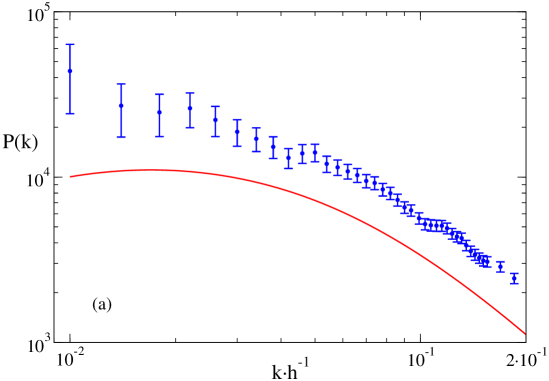
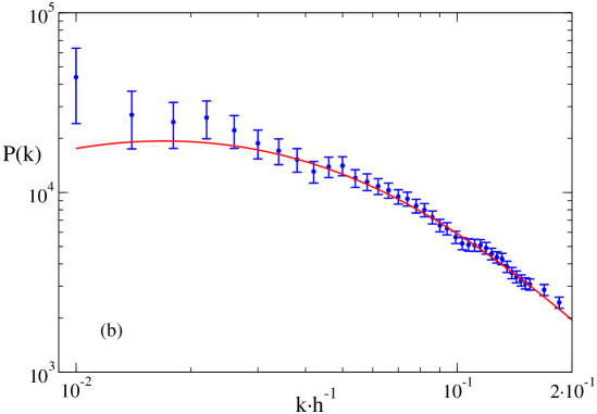
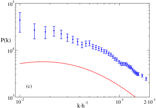
Figure 1: Baryonic power spectrum for the $\Lambda$CDM model, for fixed $\Omega_{B}^{0}=0.04$, $\Omega_{DM}^{0}=0.21$ and for (a) $\Omega_{\Lambda}^{0}=0.15$ (open Universe), (b) $\Omega_{\Lambda}^{0}=0.75$ (flat Universe) (b) and (c) $\Omega_{\Lambda}^{0}=1.25$ (closed Universe), together with the LSS data from the 2dfFGRS [8]. The ordinate axis represents $P(k)=|\delta_{m}(k)|^{2}$ at $z=0$ as given by (29) with the transfer function (31) and growth function (32), while in the abscissa we have the wave number $k$ given in $h\,$Mpc^-1 units.

In Fig. 2 we fix the values $\Omega_{B}^{0}=0.04$ and $\Omega_{\Lambda}^{0}=0.75$ and vary the dark matter content $\Omega_{DM}^{0}$ in each plot. Specifically, we plot the three cases $\Omega_{DM}^{0}=0.01,\,0.21$  and  $0.41$, representing an open, flat and closed Universe, respectively. We note that the pressureless components of the matter content (dark matter and baryons) tend to increase the power spectrum. One can see (for the given values of $\Omega_{B}^{0}$ and $\Omega_{\Lambda}^{0}$) that the best fit occurs for the expected DM content, namely around $\Omega_{DM}^{0}=0.21$ (cf. Fig. 2b). This provides further confidence in the normalization of our computation with respect to the standard $\Lambda$CDM case.

    

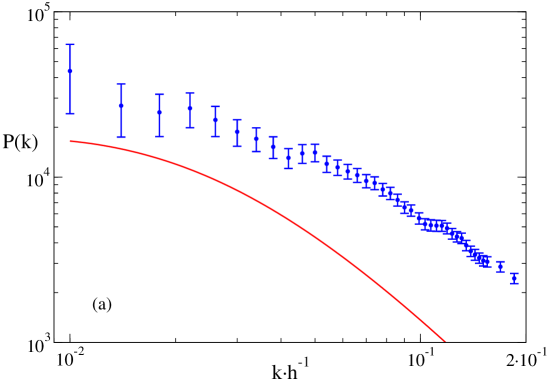
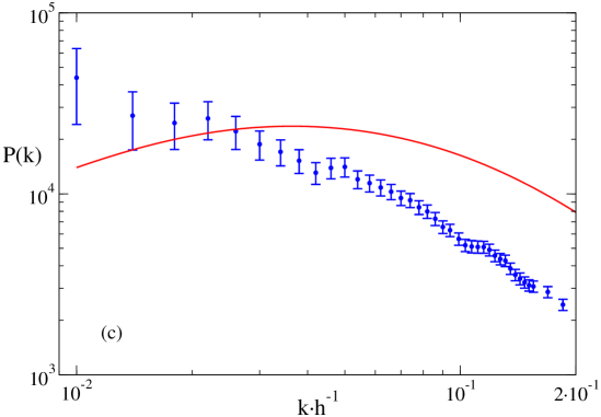
Figure 2: As in Fig 1 ($\Lambda$CDM model) for fixed $\Omega_{B}^{0}=0.04$, $\Omega_{\Lambda}^{0}=0.75$ and for (a) $\Omega_{DM}^{0}=0.11$ (open Universe), (b) $\Omega_{DM}^{0}=0.21$ (flat Universe) and (c) $\Omega_{DM}^{0}=0.41$ (closed Universe), together with the LSS data from the 2dfFGRS [8].

4.3 Power spectrum for the running $\Lambda$ case

Now we can start to deal with our main task, that is, to explore the influence of the RG parameter $\nu$ on the processed power spectrum. It is apparent that the larger is the value of $\nu$, the more important is the contribution of the function $\varrho(z)$, Eq.(25), in the solution of our set of differential equations. This function appears as a factor of the Laplacian acting on the perturbed quantities, see Eq. (18). Hence, large $\varrho(z)$ entails a more intensive damping of the perturbations contributing to depress the power spectrum. This feature can be seen at work in the plots of Fig. 3a,b,c,d. These plots illustrate the power spectrum for running $\Lambda$ in the flat case and for non-vanishing and positive $\nu$. They correspond to $\Omega_{DM}^{0}=0.21$, $\Omega_{B}^{0}=0.04$ and $\Omega_{\Lambda}^{0}=0.75$, for  $\nu=10^{-8},10^{-6}$, $10^{-4}$  and  $10^{-3}$  respectively. We can easily grasp the impact of the $\nu$ parameter, namely we see quite patently that the larger is $\nu>0$ the more suppressed is the power, mainly at small scales (i.e. at large $k$). For values of $\nu>0$ up to $\nu=10^{-6}$ the agreement with the LSS data is almost perfect; for $\nu=10^{-5}$ (not shown in the figures) the theoretical curve starts to depart maily in the high $k$ region, i.e. at small distances. Above  $\nu=10^{-4}$ the spectrum presents a strong deviation (depletion of the power) with respect to the observational data, as can be seen in Fig. 3d corresponding to $\nu=10^{-3}$. This is a quite robust result, and we can state that values of $\nu$ above $10^{-4}$ are definitely ruled out by the perturbations analysis.

The interpretation of this result in terms of particle physics can be obtained from Eq. (4), in which we recall that $M$ stands for the effective mass of the heavy particles contributing to the running of the cosmological term. Therefore, in the framework of the given model for the running CC – that is, assuming the possibility of an energy exchange between vacuum and matter sector via the conservation equation (2) – the exclusion of values $\nu>10^{-4}$ means that we can rule out the existence of particles with masses of the Planck mass order, unless their contributions to the CC cancel quite accurately due to some strong symmetry (e.g. supersymmetry).

    

    

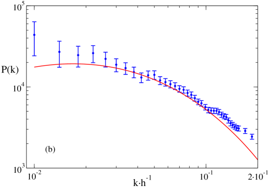
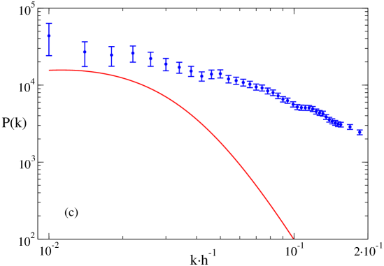
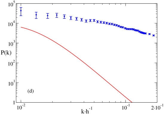
Figure 3: As in Fig 1, but for the  $\nu$-dependent power spectrum of the running cosmological constant model, together with the LSS data from the 2dfFGRS [8]. The ordinate axis represents $P(k)=|\delta_{m}(k)|^{2}$ where $\delta_{m}(k)$ is the solution of (26)-(28) at $z=0$. In all cases we have fixed $\Omega_{B}^{0}=0.04$, $\Omega_{DM}^{0}=0.21$ and $\Omega_{\Lambda}^{0}=0.75$ with the following (positive) values of $\nu$: (a) $10^{-8}$, (b) $10^{-6}$, (c) $10^{-4}$ and (d) $10^{-3}$.

On the face of the previous result, the next relevant question is: which is then the minimum upper bound on $\nu$ compatible with the observational data? It turns out that for values of $\nu>0$ between $10^{-6}$ and $10^{-4}$ (and above all between $10^{-6}$ and $10^{-5}$) it is not possible to state, at this stage, if they are definitely ruled out or not. In principle, from the inspection of Fig. 3 we could strongly argue in favor of the safer range $0\leqslant\nu\leqslant 10^{-6}$. However, we must take into account the potential effect of other components. For instance, if we increase the amount of dark matter (which is not excluded), the values of  $\nu>10^{-6}$  may lead to a better fit. On the other hand, for negative values of $\nu$ the bound becomes essentially stronger, i.e. $\nu<0$ values produce larger deviations beyond a critical range of $|\nu|$. In practice this means that for $\nu$ outside the interval $-10^{-6}\leqslant\nu\leqslant 0$ the spectrum deviates from observations more strongly than for positive values of $\nu$ outside the range $0\leqslant\nu\leqslant 10^{-6}$. This is because the parameter $\nu$  is multiplied, in the Eq. (26), by the $k^{2}$-proportional terms which stem from the pressure gradient in the perturbed equations. When the parameter $\nu$ becomes negative, the sign of the corresponding coefficient changes. This reflects in the evaluated power spectrum in the following way: while for a positive $\nu$ the spectrum is depressed in the small scale regime, for negative $\nu$ the spectrum is enhanced in that regime, and for a value of $\nu$ well below $-10^{-6}$ the spectrum becomes rapidly divergent there. This behaviour is exemplified in Fig. 4a,b,c for the cases  $\nu=-10^{-8}$, $-10^{-6}$ and $\ -10^{-4}$ respectively. In Fig. 5 we further elaborate on the $\nu<0$ features studied in the previous figure, namely we superimpose the detailed evaluation of the spectrum for the five cases $\nu=-10^{-8},-10^{-7},-10^{-6},-10^{-5}$ and $-10^{-3}$. In this way we can better appreciate the aforementioned divergence at small scales, which becomes more and more evident the larger is $|\nu|$. In fact, in this case we see that for $|\nu|>10^{-5}$ the deviation is far more pronounced than for $\nu>0$ and this demonstrates that the departure of the predicted spectrum from the experimental values in the range $\ -10^{-4}\leqslant\nu\leqslant-10^{-5}$ is much more violent than in the corresponding positive range $\ 10^{-5}\leqslant\nu\leqslant 10^{-4}$.

The change of behaviour in passing from positive to negative values of $\nu$ could be expected. It corresponds to the change of an oscillatory behaviour into an exponential one or, in other words, to the transition from a harmonic oscillator regime to an anti-harmonic oscillator regime. We can also understand why the spectrum is not essentially affected at large scales by the change of sign in $\nu$, since at large scales the pressure gradient is negligible. For negative $\nu$, the variation of the amount of dark matter and dark energy affect the final spectrum in the same way as for a positive $\nu$ case.

To summarize, the approximate range of values of the RG parameter which are amply allowed by the analysis of the matter power spectrum of perturbations (i.e. what we may call the “safest range” of allowed values of $\nu$) is the following:

$$-10^{-6}\leqslant\nu\leqslant 10^{-6}\,.$$ (37)

There are nevertheless some $\nu$ intervals outside the safest region which can still be considered allowed (or at least not ruled out) by the density perturbations analysis. For instance, positive values of $\nu$ in the range $10^{-6}-10^{-4}$ (mainly those between $10^{-6}$ and $10^{-5}$) cannot be definitely ruled out; we can only say that the corresponding spectrum starts to show some deviation from the LSS data becoming more and more acute the closer we get to $10^{-4}$. For $\nu<0$ the exclusion effect is stronger, and indeed we can safely rule out the range $\nu<-10^{-5}$ for which the predicted spectrum becomes rapidly divergent at low scales. Furthermore, for $|\nu|>10^{-4}$ the deviation is markedly patent for any sign of $\nu$ and we can assert that this range is manifestly excluded.

Finally, we may ask ourselves how to better improve the aforesaid limits on the RG parameter $\nu$. In our opinion this can only be accomplished by the simultaneous crossing of the LSS data with further observational data, most significantly with the wealth of CMB anisotropy data. This should constraint much better the value of $\nu$ beyond the LSS limits that we have been able to obtain. In particular, it would probably help to decide what is the situation with the unsettled positive range $\nu=10^{-6}-10^{-4}$ where the LSS data cannot give a last word. In principle, the CMB spectrum predicts an almost spatially flat Universe. But this result is model dependent and another full fledged direct evaluation of the cosmological parameters using the running cosmological constant model must be made. We plan to perform this analysis in the future.

    

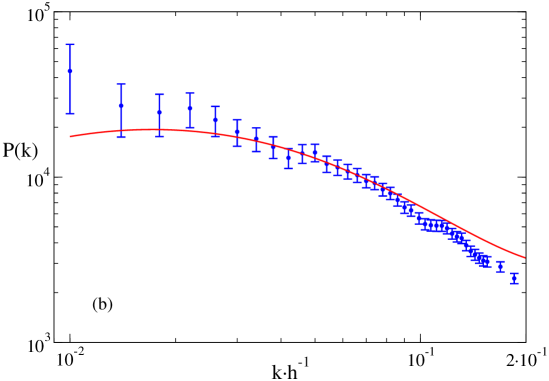
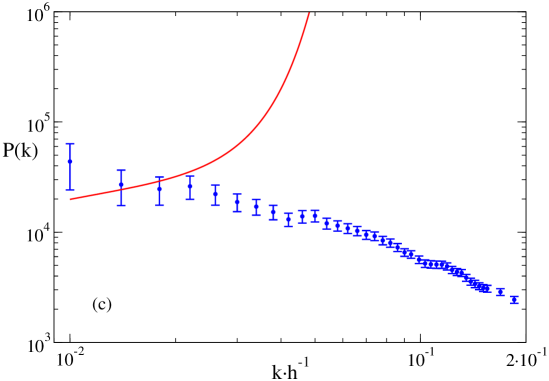
Figure 4: As in Fig 3 (running cosmological constant model), but for fixed $\Omega_{B}^{0}=0.04$, $\Omega_{DM}^{0}=0.21$ and $\Omega_{\Lambda}^{0}=0.75$ and for the following (negative) values of $\nu$: (a) $-10^{-8}$, (b) $-10^{-6}$, and (c) $-10^{-4}$, together with the LSS data from the 2dfFGRS [8].

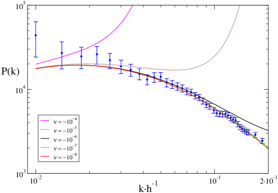
Figure 5: As in Fig 3 (running cosmological constant model), but for fixed $\Omega_{B}^{0}=0.04$, $\Omega_{DM}^{0}=0.21$ and $\Omega_{\Lambda}^{0}=0.75$ with different negative values of $\nu$ indicated in the figure, together with the LSS data from the 2dfFGRS [8]. The curves corresponding to the last two values of $\nu$ in the list almost coincide.

5 Discussion and conclusions

The possibility that the cosmological constant $\Lambda$ can be a running parameter within QFT in curved space-time was investigated extensively in  [11]. The phenomenological implications of these renormalization group (RG) cosmologies on supernovae observations have been amply addressed in different works preceding this one  [29, 30, 31, 32, 33, 34, 35, 36]. Here we have extended the analysis of phenomenological implications to the very relevant issue of structure formation. We have studied in detail the power spectrum of matter density perturbations for the FLRW type of cosmological model with running $\Lambda$. This model is characterized by a fundamental parameter $\nu$ associated to the running of $\Lambda$. At the same time this parameter acts, in the present realization of the model, as a coupling between the vacuum energy and matter (mainly CDM). There are other implementations of this framework where $\nu$ does not lead to this kind of coupling, see [34]. However, in the present work we have just focused on the original RG model [29, 32], where this coupling is present and, therefore, the cosmological term can decay into matter and vice versa. Then, under the simplifying assumptions of adiabaticity (i.e. of having no perturbations associated to entropy exchange) and of having no anisotropic stress contributions, we have derived the complete coupled set of matter density and metric perturbations for this model. The RG running of $\Lambda$ is based on the assumption of a standard quadratic decoupling law at low energies [29, 32] and we have taken the simplest covariant form of this equation – see (12) – as our ansatz to derive the perturbations. This phenomenological input leads to a cosmological model with the $H^{2}$-dependence of the vacuum energy density [11]. It is important to emphasize that this does not mean that $\Lambda\sim H^{2}$, but rather that the (renormalization group) variation of $\Lambda$ satisfies $\delta\Lambda\sim H^{2}$, and hence $\Lambda=a+b\,H^{2}$ – see Eq. (5). The effect produced by the running depends on a single parameter $\nu$, which characterizes the particle mass spectrum of the quantum theory below the Planck scale. For $\nu=0$ we retrieve the standard $\Lambda$CDM model with time-independent cosmological constant, while the values around the “canonical” value $\nu=\nu_{0}\sim 10^{-2}$ correspond to having effective particle contributions of order of the Planck mass.

The numerical analysis of the perturbations proves to be in qualitative agreement with the results of the previous estimate in Ref. [40], based on restraining the amplification of the density fluctuating spectrum at the recombination era caused by the vacuum decay into CDM. In both cases (viz. the direct calculation and the previous estimate) it is found that the “canonical” value of $\nu$ leads to strong deviations from the observational data. For positive values of $\nu$ in the range $10^{-6}\leqslant\nu\leqslant 10^{-5}$, corresponding approximately to the GUT particle spectrum ($M_{X}\sim(10^{-2}-10^{-3})\,M_{P}$), we meet relatively small deviations of the theoretical curve from the $\nu=0$ case. The deviations are higher the larger is $|\nu|$. Let us recall that the upper bound on $\nu$ obtained from the phenomenological estimate of [40] is $10^{-3}$ and applies only for $\nu\geqslant 0$. This bound is not very far away from our own most conservative result $|\nu|<10^{-4}$, although in our case it applies for both signs of $\nu$. Moreover, the approximate bound is much weaker than the one defined by the so-called “safest $\nu$ range” – cf. Eq.  (37). However, as we already emphasized, we cannot definitely exclude the $\nu>0$ interval $10^{-6}-10^{-4}$ (and specially the subinterval $10^{-6}-10^{-5}$). Therefore, we may assert, in the most possible conservative way, that our direct bounds on $\nu>0$ are between one to two orders of magnitude more restrictive than those of [40], but of course they have been derived in a much more rigorous way. Let us also remark that our exclusion of the possibility that $\nu$ could be of the order of magnitude of the “canonical” value $\nu_{0}\sim 10^{-2}$ is at variance (by at least two orders of magnitude) with the estimates obtained from the approximate methods used in references [41, 42] .

It is also interesting to compare our results with those of Ref. [47], where a detailed study of matter density perturbations in interacting quintessence models is addressed. These authors perform their study also under the assumption of an adiabatic regime and with no contributions from anisotropic stress. In this kind of modified quintessence models, first proposed in  [54], one couples matter to quintessence by means of a source function $Q$ which depends on a free parameter, called $c^{2}$ in Ref. [47]. This is the only free parameter in that model, similarly as is $\nu$ in our own framework under the specified common set of assumptions. In the models of interactive quintessence, the dark energy (DE) can also decay into matter (parallel to our case where $\Lambda$ can also decay into matter) and as a result the amount of DE in the past is larger than in ordinary quintessence models with self-conserved DE. This corresponds, in our framework, to have $\nu>0$ because then $\Lambda$ becomes larger in the past. The authors of  [47] find that the effect of the $c^{2}$-coupling is to introduce a damping of the power spectrum of matter perturbations at low scales; that is to say, the growth of density perturbations for large wave numbers becomes smaller as compared to quintessence models with uncoupled DE to matter. In our RG framework, we observed a similar depletion of the spectrum at low scales for $\nu>0$ as compared to $\nu=0$ (the standard $\Lambda$CDM model) – cf. sections 4.2 and 4.3. Moreover, we have found numerical bounds on $\nu$ that are quantitatively similar, in fact a bit more stringent than those on $c^{2}$ obtained in the model of  [47]. These authors found that their power spectrum is consistent with the 2dFGRS data provided $c^{2}\leq 10^{-3}$, and we find that the largest allowed value of $\nu$ by the same LSS data is of order $10^{-4}$. The basic agreement among the different analyses suggest that the loss of power at low scales could be a general feature of dynamical models in which the dark energy decays into matter during the cosmic evolution. The latter situation is always the case in Ref.  [47] because $c^{2}>0$, and it is also our case for $\nu>0$. However, in our RG framework, $\nu$ can have any sign (depending on the dominance of bosons or fermions in the loop contributions to the running of $\Lambda$) and so we have an opportunity to explore also the case $\nu<0$. For this sign of $\nu$, the running $\Lambda$ becomes progressively smaller in the past and reaches eventually large negative values (see the detailed evolution plots of Ref. [32]). As a result we may expect an overproduction of structure associated to the fact that a large negative $\Lambda$ increases the gravitational collapse. Since, however, this is not observed (cf. the plots of section 4.3 detecting an excess of power at low scales for $\nu<0$), this may provide a physical explanation of why negative values of $\nu$ are significantly more restrained. While the safest and most stringent range of values of $\nu$ is expressed in a nutshell in Eq. (37), we cannot exclude that $|\nu|$ could be higher (mainly in the $\nu>0$ case) once it will be possible to combine the analysis of the matter power spectrum with the corresponding CMB analysis. At the same time, we should recall that the bounds obtained on $\nu$ in our case, and on $c^{2}$ in  [47], could suffer some renormalization if we would abandon the set of simplifying hypotheses that have been made. However, our study shows at least the kind of impact to be expected on the matter power spectrum predicted by cosmological models with running $\Lambda$ in interaction with matter. Further investigations would be needed to assess the effect in a more thorough way, but they lie beyond the scope of the present work.

Let us also finally remark that the bounds we have placed on the RG parameter $\nu$, within our set of assumptions, can be interpreted on purely phenomenological grounds, namely as bounds on a parameter that gauges the possible degree of interaction between CDM and the vacuum energy, even if no fundamental RG model is invoked. In principle, the phenomenological implications of a non-vanishing $\nu$ could be potentially detectable in the future supernovae observations, either through a direct measure of the running of $\Lambda$  [32, 33] or (more efficiently in practice) through the possibility to observe the redshift evolution of the effective equation of state parameter associated to the variable CC model  [35, 36]. However, the very study of the evolution of the density and metric perturbations, which has led us to firmly exclude the range $|\nu|>10^{-4}$, already demonstrates the difficulty of the previous methods and at the same time emphasizes the great advantage of the density perturbations approach. Indeed, the strong sensitivity of the matter power spectrum to a variable cosmological term interacting with the CDM shows that this is perhaps the ideal observable to look at. Therefore, future data on LSS could eventually provide the clue to unravel an interaction (even if very small) between matter (essentially CDM) and vacuum, and at the same time it may hint at the possible RG physics behind it. Let us conclude by mentioning that it should be very interesting to expand our analysis to the aforementioned second model of running CC [34]. In this alternate model the cosmological term is also evolving in time and redshift, but there is no energy exchange between matter and vacuum and we may expect much more freedom in choosing the value of $\nu$. We leave this study for a future publication.

Acknowledgments: We are grateful to Jérôme Martin for useful discussions, to Hrvoje Štefančić for checking our numerical code and for interesting discussions, and finally to Javier Grande for his aid in improving the presentation of our plots and also for useful discussions. The work of J.C.F has been supported in part by CNPq (Brazil) and by CAPES/COFECUB Brazilian-French scientific cooperation. The work of I.Sh. has been supported in part by the grants from CNPq (Brazil), FAPEMIG (Minas Gerais, Brazil) and ICTP (Italy). The work of J.S. has been partially supported by MECYT and FEDER under project 2004-04582-C02-01, and also by DURSI Generalitat de Catalunya under project 2005SGR00564.

References

- [1] P.J.E. Peebles, Physical Principles of Cosmology (Princeton University Press, 1993); T. Padmanabhan, Structure formation in the Universe (Cambridge University Press, 1993); J.A. Peacock, Cosmological Physics (Cambridge Univ. Press, 1999).
- [2] A. R. Liddle, D.H. Lyth, Cosmological Inflation and Large Scale Structure (Cambridge Univ. Press, 2000); S. Dodelson, Modern Cosmology (Academic Press, 2003); V. Mukhanov, Physical Foundations of Cosmology (Cambridge Univ. Press, 2005).
- [3] S. Weinberg, Gravitation and Cosmology (John Wiley and Sons. Inc., 1972).
- [4] A.G. Riess et al., Astronom. J. 116 (1998) 1009; S. Perlmutter et al., Astrophys. J. 517 (1999) 565; R. A. Knop et al., Astrophys. J. 598 102 (2003); A.G. Riess et al. Astrophys. J. 607 (2004) 665.
- [5] P. de Bernardis et al., Nature 404 (2000) 955; C.B. Netterfield et al. (Boomerang Collab.), Astrophys. J. 571 (2002) 604; N.W. Halverson et al., Astrophys. J. 568 (2002) 38.
- [6] C.L. Bennett et al., Astrophys.J.Suppl. 148 (2003) 1; D.N. Spergel et al., Astrophys. J. Suppl. 148 (2003) 175, astro-ph/0302209; D. N. Spergel et al., Astrophys. J. Suppl. 148 (2003) 175.
- [7] D.N. Spergel et al., WMAP three year results: implications for cosmology, astro-ph/0603449.
- [8] S. Cole et al, Mon. Not. Roy. Astron. Soc. 362 (2005) 505-534, astro-ph/0501174.
- [9] M. Tegmark et al., Phys. Rev. D69 (2004) 103501, astro-ph/0310723.
- [10] S. Weinberg, Rev. Mod. Phys., 61 (1989) 1.
- [11] I. Shapiro, J. Solà, JHEP 0202 (2002) 006, hep-th/0012227.
- [12] I. Shapiro, J. Solà, Phys. Lett. 475B (2000) 236, hep-ph/9910462.
- [13] A.D. Dolgov, in: The very Early Universe, Ed. G. Gibbons, S.W. Hawking, S.T. Tiklos (Cambridge U., 1982); F. Wilczek, Phys. Rev. D104 (1984) 143; T. Banks, Nucl. Phys. B249(1985)332; R.D. Peccei, J. Solà, C. Wetterich, Phys. Lett. B195 (1987) 183; J. Solà, Phys. Lett. B228 (1989) 317.
- [14] See e.g. V. Sahni, A. Starobinsky, Int. J. of Mod. Phys. 9 (2000) 373; S.M. Carroll, Living Rev. Rel. 4 (2001) 1; T. Padmanabhan, Phys. Rep. 380 2003 235; J. Solà, Nucl. Phys. Proc. Suppl. 95 (2001) 29; S. Nobbenhuis, The Cosmological Constant Problem, an Inspiration for New Physics, gr-qc/0609011.
- [15] E.J. Copeland, M. Sami, S. Tsujikawa, Dynamics of dark energy, hep-th/0603057.
- [16] P.J.E. Peebles, B. Ratra, Rev. of Mod. Phys. 75 (2003) 559.
- [17] U. Alam, V. Sahni, A.A. Starobinsky, JCAP 0406 (2004) 008; H.K. Jassal, J.S. Bagla, T. Padmanabhan, Mon. Not. Roy. Astron. Soc. Letters 356 (2005) L11-L16; Phys. Rev. D 72(2005) 103503.
- [18] H.K. Jassal, J.S. Bagla, T. Padmanabhan, astro-ph/0601389; K. M. Wilson, G. Chen, B. Ratra, astro-ph/0602321; S. Nesseris, L. Perivolaropoulos, Phys. Rev. D 73 (2006)103511; G.B Zhao, J.Q. Xia, B. Feng, X. Zhang , astro-ph/0603621; L. Samushia, B. Ratra, astro-ph/0607301; J.Q. Xia, G.B. Zhao, H. Li, B. Feng, X. Zhang, astro-ph/0605366.
- [19] R.R. Caldwell, R. Dave, P.J. Steinhardt, Phys. Rev. Lett. 80 (1998) 1582; P.J.E. Peebles, B. Ratra, Astrophys. J. Lett. 325 L17 (1988); C. Wetterich, Nucl. Phys. B302 (1988) 668; A. R. Liddle, Rev. Mod. Phys. 75(2003) 599; C. Armendariz-Picon, V. Mukhanov, P.J. Steinhardt, Phys. Rev. D 63 (2001) 103510; M. Malquarti, E.J. Copeland, A. R. Liddle, Phys. Rev. D68 (2003) 023512.
- [20] A.Yu. Kamenshchik, U. Moschella, V. Pasquier Phys. Lett. 511B (2001) 265; M.C. Bento, O. Bertolami, A.A. Sen, Phys. Rev. 66D (2002) 043507; J.C. Fabris, S.V.B. Gonçalves, P.E. de Souza, Gen. Rel. Grav. 34 (2002) 53.
- [21] C. Deffayet, G. Dvali, G. Gabadadze, Phys. Rev. D65 (2002) 044023.
- [22] T.R. Taylor and G. Veneziano, Nucl. Phys. 345B (1990) 210.
- [23] A.M. Polyakov, Int. J. Mod. Phys. 16 (2001) 4511.
- [24] I. Antoniadis, E. Mottola, Phys.Rev. D45 (1992) 2013.
- [25] A. Bonanno, M. Reuter, Phys. Rev. D 65 (2002) 043508; Int. J. Mod. Phys. D13 (2004) 107; E. Bentivegna, A. Bonanno, M. Reuter, JCAP 0401 (2004) 001; B.F.L. Ward, Int. J. of Mod. Phys. A20 (2005) 3258.
- [26] I.L. Buchbinder, S.D. Odintsov and I.L. Shapiro, Effective Action in Quantum Gravity, IOP Publishing (Bristol, 1992); N.D. Birrell and P.C.W. Davies, Quantum Fields in Curved Space, Cambridge Univ. Press (Cambridge, 1982).
- [27] I.L. Shapiro, Phys. Lett. 329B (1994) 181.
- [28] E.V. Gorbar, I.L. Shapiro, JHEP 02 (2003) 021; JHEP 06 (2003) 004; JHEP 02 (2004) 060.
- [29] I.L. Shapiro, J. Solà, C. España-Bonet, P. Ruiz-Lapuente, Phys. Lett. B 574 (2003) 149, astro-ph/0303306.
- [30] I.L. Shapiro, J. Solà, Nucl. Phys. Proc. Suppl. 127 (2004) 71, hep-ph/0305279.
- [31] A. Babić, B. Guberina, R. Horvat and H. Štefančić, Phys. Rev. D65 (2002) 085002; B. Guberina, R. Horvat and H. Štefančić, Phys. Rev. D67 (2003) 083001; A. Babić, B. Guberina, R. Horvat, H. Štefančić, Phys. Rev. D71 (2005) 124041.
- [32] C. España-Bonet, P. Ruiz-Lapuente, I.L. Shapiro, J. Solà, JCAP 02 (2004) 006, hep-ph/0311171.
- [33] I. L. Shapiro, J. Solà, JHEP proc. AHEP2003/013, astro-ph/0401015.
- [34] I. L. Shapiro, J. Solà, H. Štefančić, JCAP 0501 (2005) 012, hep-ph/0410095.
- [35] J. Solà, H. Štefančić, Phys. Lett. B 624 (2005) 147, astro-ph/0505133.
- [36] J. Solà, H. Štefančić, Mod. Phys. Lett. A21 (2006) 479, astro-ph/0507110; J. Solà, H. Štefančić, J. Phys. A 39 (2006) 6753, gr-qc/0601012; J. Solà, J. Phys. Conf. Ser. 39 (2006) 179, gr-qc/0512030.
- [37] J. Grande, J. Solà, H. Štefančić, JCAP 08 (2006) 011, gr-qc/0604057; gr-qc/0609083 (Phys. Lett. B, in press).
- [38] J. D. Barrow, T. Clifton, Phys. Rev. D 73 (2006) 103520.
- [39] F. Bauer, Class. Quant. Grav. 22 (2005) 3533, gr-qc/0501078; gr-qc/0512007.
- [40] R. Opher, A. Pelinson, Phys. Rev. D70 (2004) 063529, astro-ph/0405430.
- [41] P. Wang, X.H. Meng, Class. Quant. Grav. 22 (2005) 283, astro-ph/0408495.
- [42] J. S. Alcañiz, J.A.S. Lima, Phys. Rev. D72 (2005) 063516, astro-ph/0507372.
- [43] O. Lahav et al., Mon. Not. Roy. Astron. Soc 333 (2002) 961.
- [44] T. Appelquist and J. Carazzone, Phys. Rev. D11 (1975) 2856.
- [45] J. Ren, X.H. Meng, Phys. Lett. B 636 (2006) 5.
- [46] R. Opher, A. Pelinson, Mon. Not. Roy. Astron. Soc. 362 (2005) 167, astro-ph/0409451.
- [47] G. Olivares, F. Atrio-Barandela and D. Pavon, Phys. Rev. D74 (2006) 043521.
- [48] J.C. Fabris, Ph. Spindel, Phys. Rev. D64 (2001) 084007.
- [49] J. Martin, A. Riazuelo and M. Sakellariadou, Phys. Rev. D61 (2000) 083518.
- [50] N. Sugiyama, Astrophys. J.Suppl. 100 (1995) 281, astro-ph/9412025.
- [51] J.M. Bardeen, J.R. Bond, N. Kaiser and A.S. Szalay, Astrophys. J. 304 (1986) 15.
- [52] S. M. Carroll, W, H. Press, E. L. Turner, Ann. Rev. Astron. Astrophys. 30 (1992) 499.
- [53] G. Hinshaw et al., Three-Year Wilkinson Microwave Anisotropy Probe (WMAP) Observations: Temperature Analysis, astro-ph/0603451.
- [54] L. Amendola, Phys. Rev. D62 (2000) 043511.