ITP-UU-06/34
SPIN-06/30
gr-qc/yyxxxxx
The Cosmological
Constant Problem,
an Inspiration for New Physics
Stefan Nobbenhuis
Ph.D. Thesis, defended June 15. 2006
Supervisor: Prof. Dr. G. ’t Hooft.
Institute for Theoretical Physics
Utrecht University, Leuvenlaan 4
3584 CC Utrecht, the Netherlands
and
Spinoza Institute
Postbox 80.195
3508 TD Utrecht, the Netherlands
S.J.B.Nobbenhuis@phys.uu.nl
We have critically compared different approaches to the cosmological constant problem, which is at the edge of elementary particle physics and cosmology. This problem is deeply connected with the difficulties formulating a theory of quantum gravity. After the 1998 discovery that our universe’s expansion is accelerating, the cosmological constant problem has obtained a new dimension. We are mainly interested in the question why the cosmological constant is so small. We have identified four different classes of solutions: a symmetry, a back-reaction mechanism, a violation of (some of) the building blocks of general relativity, and statistical approaches.
In this thesis we carefully study all known potential candidates for a solution, but conclude that so far none of the approaches gives a satisfactory solution. A symmetry would be the most elegant solution and we study a new symmetry under transformation to imaginary spacetime.
Chapter 1 The Cosmological Constant Problem
In this chapter we carefully discuss the different aspects of the cosmological constant problem. How it occurs, what the assumptions are, and where the difficulties lie in renormalizing vacuum energy. Different interpretations of the cosmological constant have been proposed and we briefly discuss these. We subsequently, as a warm-up, point at some directions to look at for a solution, before ending this chapter by giving an outline of the rest of the thesis.
1.1 The ‘Old’ Problem, Vacuum Energy as Observable Effect
In quantum mechanics, the energy spectrum, , of a simple harmonic oscillator111See Appendix A for conventions and some definitions used throughout this thesis, e.g. . is given by . The energy of the ground state, the state with lowest possible energy, is non-zero, contrary to classical mechanics. This so-called zero-point energy is usually interpreted by referring to the uncertainty principle: a particle can never completely come to a halt.
Free quantum field theory is formulated as an infinite series of simple harmonic oscillators. The energy density of the vacuum in for example free scalar field theory therefore receives an infinite positive contribution from the zero-point energies of the various modes of oscillation:
| (1.1) |
and we set . With a UV-cutoff , regularizing the a priori infinite value for the vacuum energy density, this integral diverges222This is just the leading divergence, see section (1.3) for a more precise discussion. as .
The filling of the ‘Dirac sea’ in the quantization of the free fermion theory leads to a downward shift in the vacuum energy with a similar ultraviolet divergence. The Hamiltonian is:
| (1.2) |
where the creates negative energy. Therefore we have to require that these operators satisfy anti-commutation relations:
| (1.3) |
since this is symmetric between and , we can redefine the operators as follows:
| (1.4) |
which obey the same anti-commutation relations. Now the second term in the Hamiltonian becomes:
| (1.5) |
Now we choose to be the vacuum state that is annihilated by the and and all excitations have positive energy. All the negative energy states are filled; this is the Dirac sea. A hole in the sea corresponds to an excitation of the ground state with positive energy, compared to the ground state. The infinite constant contribution to the vacuum energy density has the same form as in the bosonic case, but enters with opposite sign.
Spontaneous symmetry breaking gives a finite but still possibly large shift in the vacuum energy density. In this case,
| (1.6) |
where the potential is given by:
| (1.7) |
where and both are positive constants and is a constant with arbitrary sign. The potential is at its minimum value for , leading to a shift in the energy density of the ground state:
| (1.8) |
The spontaneous breaking of the weak interaction symmetry and of the strong interaction chiral symmetry both would be expected to shift the vacuum energy density in this way. Through the additive constant the minimum of the potential either after, or before symmetry breaking, can be tuned to any value one likes, but within field theory, this value is completely arbitrary.
More generally, in elementary particle physics experiments, the absolute value of the vacuum energy is unobservable. Experimentally measured particle masses, for example, are energy differences between the vacuum and certain excited states of the Hamiltonian, and the absolute vacuum energy cancels out in the calculation of these differences.
In GR however, each form of energy contributes to the energy-momentum tensor , hence gravitates and therefore reacts back on the spacetime geometry, as can be seen from Einstein’s equations:
| (1.9) |
As it stands, the cosmological constant is a free parameter that can be interpreted as the curvature of empty spacetime. However, Lorentz invariance tells us that the energy-momentum tensor of the vacuum looks like:
| (1.10) |
since the absence of a preferred frame for the vacuum means that must be the same for all observers connected by Lorentz transformations. Apart from zero, there is only one isotropic tensor of rank two, which is the metric tensor. If we move the CC term to the right-hand-side of the equation (1.9), it looks exactly the same:
| (1.11) |
This interpretation of a cosmological constant measuring the energy density of the vacuum, was first explicitly given by Zel’dovich in 1968 [1, 2].
We can therefore define an effective cosmological constant333Note that using this definition we use units in which the cosmological constant has dimension throughout.:
| (1.12) |
The vacuum energy density calculated from normal quantum field theory thus has a potentially significant observable effect through the coupling with gravity. It contributes to the effective cosmological constant and an infinite value would possibly generate an infinitely large spacetime curvature through the semiclassical Einstein equations:
| (1.13) |
Note at this point that only the effective cosmological constant, , is observable, not , so the latter quantity may be referred to as a ‘bare’, or perhaps classical quantity that has to be ‘dressed’ by quantum corrections, analogously to all other physical parameters in ordinary quantum field theory. If one believes quantum field theory to be correct all the way up to the Planck scale, at GeV, then this scale provides a natural ultraviolet cutoff to all field theory processes like eqn. (1.1). Such a cutoff however, would lead to a vacuum energy density of , which is roughly 123 orders of magnitude larger than the currently observed value:
| (1.14) |
This means that the bare cosmological constant has to be fine-tuned to a stunning 123 decimal places, in order to yield the correct physical result444This often mentioned factor 120, depends on the dimension used for energy density. In Planckian units, the factor 120 is the correct one, relating dimensionless numbers.. As is well known, even if we take a TeV scale cut-off the difference between experimental and theoretical results still requires a fine-tuning of about 50 orders of magnitude. Even a cutoff at for example the QCD scale (at MeV), worrying only about zero-point energies in quantum chromodynamics, would not help much; such a cutoff would still lead to a discrepancy of about 40 orders of magnitude. The answer clearly has to lie somewhere else. Even non-perturbative effects, like ordinary QCD instantons, would give far too large a contribution if not cancelled by some fundamental mechanism.
Physicists really started to worry about this in the mid-seventies, after the success of spontaneous symmetry breaking. Veltman [3] in 1975 “… concluded that this undermines the credibility of the Higgs mechanism.”
We have no understanding of why the effective cosmological constant, is so much smaller than the vacuum energy shifts generated in the known phase transitions of particle physics, and so much smaller again than the underlying field zero-point energies. No symmetry is known that can protect the cosmological constant to such a small value555See however chapter (4) for an attempt.. The magnificent fine-tuning needed to obtain the correct physical result seems to suggest that we miss an important point. In this thesis we give an overview of the main ideas that have appeared in trying to figure out what this point might be. For instance, one might suspect that it was naive to believe that vacuum energy, like any other form of energy contributes to the energy-momentum tensor and gravitates. It is however an assumption that is difficult to avoid.
In conclusion, the question is why is the effective cosmological constant so close to zero? Or, in other words, why is the vacuum state of our universe (at present) so close to the classical vacuum state of zero energy, or perhaps better, why is the resulting four-dimensional curvature so small, or why does Nature prefer a flat spacetime? Apparently spacetime is such, that it takes a lot of energy to curve it, while stretching it is (almost) for free, since the cosmological constant is (almost) zero. This is quite contrary to properties of objects from every day experience, where bending requires much less energy than stretching.
As a nice example, Pauli in the early 1920’s was way ahead of his time when he wondered about the gravitational effect of the zero-point energy of the radiation field. He used a cutoff for the radiation field at the classical electron radius and realized that the entire universe “could not even reach to the moon” [4]. The calculation is straightforward and also restated in [5]. The vacuum energy-density of the radiation field is:
| (1.15) |
With the cutoff . This implies for the radius of the universe:
| (1.16) |
indeed far less then the distance to the moon.
Nobody else seems to have been bothered by this, until the late 1960’s when Zel’dovich [1, 2] realized that, even if one assumes that the zero-point contributions to the vacuum energy density are exactly cancelled by a bare term, there still remain very problematic higher order effects. On dimensional grounds the gravitational interaction between particles in vacuum fluctuations would be of order , with some cutoff scale. This corresponds to two-loop Feynman diagrams. Even for as low as 1 GeV, this is about 9 orders of magnitude larger than the observational bound.
This illustrates that all ’naive’ predictions for the vacuum energy density of our universe are greatly in conflict with experimental facts, see table (1.1) for a list of order-of-magnitude contributions from different sources. All we know for certain is that the unification of quantum field theory and gravity cannot be straightforward, that there is some important concept still missing from our understanding. Note that the divergences in the cosmological constant problem are even more severe than in the case of the Higgs mass: The main divergences here are quartic, instead of quadratic. It is clear that the cosmological constant problem is one of the major obstacles for quantum gravity and cosmology to further progress.
| Observed | ||
|---|---|---|
| Quantum Field Theory | ||
| Quantum Gravity | ||
| Supersymmetry | ||
| Higgs Potential | ||
| Other Sources |
1.1.1 Reality of Zero-Point Energies
The reality of zero-point energies, i.e. their observable effects, has been a source of discussion for a long time and so far without a definite conclusion about it. Besides the gravitational effect in terms of a cosmological constant, there are two other observable effects often ascribed to the existence of zero-point energies: the Lamb shift and the Casimir effect.
A recent investigation by Jaffe [6] however, concluded that neither the experimental confirmation of the Casimir effect, nor of the Lamb shift, established the reality of zero-point fluctuations. However, no completely satisfactory description of, for example QED, is known in a formulation without zero-point fluctuations.
Note that in the light-cone formulation, a consistent description of e.g. QED can be given, with the vacuum energy density automatically set to zero. This is accomplished by selecting two preferred directions, and thus breaks Lorentz invariance. However, there is no physical reason to select these coordinates, and moreover, a discussion of tadpole diagrams and cosmological terms in de Sitter spacetime becomes problematic in these coordinates.
1.1.2 Repulsive Gravity
A positive cosmological constant gives a repulsive gravitational effect. This can easily be seen by considering the static gravitational field created by a source mass at the origin, with density . For weak fields is the usual Lorentz metric. If we further assume a non-relativistic regime with the -component of the Einstein equation reads:
| (1.17) |
In the non-relativistic case we also expect that which is equivalent to saying that we neglect pressure and stress compared to matter density. Therefore we can set , implying and thus the curvature scalar becomes: or . Substituting this back in the equation for the component we find:
| (1.18) |
Furthermore we can derive that within our approximation . Finally recalling that Newton’s potential is related to the deviation of the -component of the metric tensor from (through ) we are led to the equation:
| (1.19) |
This is of course nothing but Poisson’s equation for the Newton potential with an additional term from the CC whose sign depends on that of . For the original gravitational field is diminished as though there were an additional repulsive interaction. These features are confirmed by explicitly solving the above equation:
| (1.20) |
We are thus led to the expected gravitational potential plus a new contribution which is like a “harmonic oscillator” potential, repulsive for .
1.2 Two Additional Problems
Actually, after the remarkable discoveries and subsequent confirmations starting in 1997 (SN)[7, 8, 9, 10, 11, 12, 13, 14, 15, 16, 17] (WMAP) [18, 19] (Boomerang) [20, 21] (SdSS) [22, 23] (Hubble) [24] that the universe really is accelerating its expansion (more about this in the next chapter), there appear to be at present at least three cosmological constant problems.
The first, or sometimes called “old” cosmological constant problem is why is the effective cosmological constant so incredibly small, as described in the previous section.
The second problem is, if it is so small, then why is it not exactly equal to zero? Often in physics it is a lot easier to understand why a parameter is identically zero, than why it is a very small number.
And a third question may be posed, based on the measured value of the effective cosmological constant. The energy density of the vacuum that it represents, appears to be of the same order of magnitude as the present matter energy density in the universe. This is quite peculiar, since, as we we will see in chapter (2), vacuum energy density, denoted , remains constant during the evolution of the universe, whereas the matter energy density, obviously decreases as the universe grows larger and larger. If the two energy densities are of the same order of magnitude nowadays, this means that their ratio, had to be infinitesimal in the early universe, but fine-tuned to become equal now. Therefore, one obviously starts to wonder whether we are living in some special epoch, that causes these two forms of energy density to be roughly equal in magnitude. This has become known as the “cosmic coincidence problem” and is also sometimes phrased as the “Why now?” problem. In this thesis we mainly concentrate on the first problem.
1.3 Renormalization
In quantum field theory the value of the vacuum energy density has no observational consequences. We can simply rescale the zero point of energy, which amounts to adding or subtracting a constant to the action, without changing the equations of motion. It can also be done more elegantly, by a book-keeping method called “normal ordering”, denoted by placing a quantity between semicolons, i.e. . In this prescription, one demands that wherever a product of creation and annihilation operators occurs, it is understood that all creation operators stand to the left of all annihilation operators. This differs from the original notation by commutator terms which renormalize vacuum energy and mass, since:
| (1.21) |
However, it is not a very satisfactory way of dealing with the divergences, considering that we have seen that vacuum energy is observable, when we include gravity. By way of comparison, we note that in solid state physics, through X-ray diffraction, zero-point energy is measurable. Here, a natural UV-cutoff to infinite integrals like (1.1) exists, because the system is defined on a lattice. And indeed, this zero-point energy turns out to be per mode.
So let us return to eqn. (1.1). In fact, there are not just quartic divergences in the expression for the vacuum energy, but also quadratic and logarithmic ones. More precisely, for a field with spin :
| (1.22) | |||||
where we have imposed an ultraviolet cutoff to the divergent integral. This shows that quartic divergences to the vacuum energy come from any field, massive or massless666It should be noted however, that since this cutoff is only on spatial momenta, it violates Lorentz invariance. It was shown in [25, 26] that the quartic divergence for the energy density and pressure of a free scalar field in fact do not describe vacuum energy, but a homogeneous sea of background radiation. However, when one does the calculation correctly, the quartic divergences are again recovered [27]. When evaluating the integral using dimensional regularization, one finds: ; no quartic or quadratic term..
In combination with gravity, these divergences must be subtracted, as usual, by a counterterm, a ‘bare’ cosmological constant, as we will see in the following. Then there are quadratic and logarithmic divergences, but these only arise for massive fields. The quadratic divergences have to be treated in the same way as the quartic ones. The logarithmic divergences are more problematic, because, even after having been cancelled by counterterms, their effect is still spread through the renormalization group. Since the theory is not renormalizable, the infinities at each loop order have to be cancelled separately with new counterterms, introducing new free parameters in the theory. Because of dimensional reasons, the effects of these new terms are small, and are only felt in the UV. However, this is an unsatisfactory situation, since much predictability is lost. Moreover, knowledge from the past has taught us that this signals that we do not understand the short distance behavior of the theory, so clearly something better is needed.
The subtraction procedure between bare terms and quantum corrections depends on the energy scale in the divergent integral. The renormalization of the cosmological constant therefore must be performed such that at energy scales where it is measured today, we get the observed value. The renormalization condition, in other words, has to be chosen at some fixed energy scale . For the cosmological constant the renormalization condition becomes:
| (1.23) |
where is the observable, physical cosmological constant, is the bare cosmological constant in Einstein’s equations, and are the quantum corrections. The coupling constants of the theory become a function of , where is called the renormalization scale. Physical observables must be independent of and this is expressed by the renormalization group equations, or more precisely, the one-dimensional subgroup of scale transformations, sending , with some constant.
Despite the fact that there exists no renormalizable theory combining gravity and particle physics, the hope is that under certain restrictions, these considerations still make sense. It has been tried, in vain, to argue that this type of running with energy scale under the renormalization group, could explain the very small value nowadays. We will discuss this scenario in section (5.3).
The restrictions mentioned above are quite severe. General relativity is a non-linear theory, which implies that gravitons not only transmit the force of gravity, but also set up a gravitational field themselves, similar, mutatis mutandis, to gluons in QCD. Gravitons ‘feel’ a gravitational field just as much as for example photons do. The approach usually taken, also in most parts of this thesis, is to consider these graviton contributions as a metric perturbation on a background spacetime, , where represents the gravitons, or gravitational waves. The gravitational waves are then treated as a null fluid, and considered to contribute to the energy momentum tensor, i.e. to the right-hand-side of Einstein’s equation, instead of the left-hand-side. The combined action for gravity and matter fields can be expanded in both and , and Feynman rules can be derived, see e.g. the lectures by Veltman [28].
As discussed above, at higher orders the gravitational corrections are out of control. However, if one truncates the expansion at a finite number of loops, then the finite number of divergent quantities that appear can be removed by renormalizing a finite number of physical quantities, see e.g. [29, 30, 31] for a more detailed description of this setup.
This procedure provides a way to use the semi-classical Einstein equations:
| (1.24) |
where is the quantum expectation value of the energy momentum tensor. For this to make any sense at all, usually the expansion is truncated already at one-loop level. In this semi-classical treatment, the gravitational field is treated classically, while the matter fields, including the graviton to one-loop order, are treated quantum mechanically.
To say something meaningful about one now has to renormalize this parameter, since the expectation value in principle diverges terribly. To do this in a curved background is not trivial. First one has to introduce a formal regularization scheme, which renders the expectation value finite, but dependent on an arbitrary regulator parameter. Several choices for regularization are available, see e.g. [30].
One option is to separate the spacetime points at which the fields in are evaluated and then average over the direction of separation. This is a covariant regularization scheme which leaves dependent on an invariant measure of the distance between the two points. The price to pay for any regularization scheme is the breaking of conformal invariance, so massless fields no longer have traceless stress-tensors. Often this distance is chosen to be one-half times the square of the geodesic distance between them, denoted by . Asymptotically, the regularized expression then becomes:
| (1.25) |
where and are constants, is the Einstein tensor and the are covariantly conserved tensors, quadratic in the Riemann tensor. So this gives a correction to the bare cosmological constant present in the Einstein-Hilbert action (term linear in ), a correction to Newton’s constant (term ) plus higher order corrections to . The tensors are the functional derivatives with respect to the metric tensor of the square of the scalar curvature and of the Ricci tensor, respectively. With the Euler-derivative, one arrives at (see e.g. [30]):
| (1.26) | |||||
and
| (1.27) | |||||
The divergent parts of can then be taken into account by adding counterterms to the standard Einstein-Hilbert action:
| (1.28) |
We did not include a term , since it can be absorbed in the other counterterms, using that the combination:
| (1.29) |
is a topological invariant and does not affect the field equations. Furthermore, in pure gravity, with no matter fields, the Einstein equations tell us that and . In this case the counterterms are unphysical, which means, together with the observation that (1.29) is a topological invariant, that pure gravity has no infinities at one-loop level and thus is one-loop renormalizable.
If we now again include the matter action and vary both with respect to the metric in order to obtain the field equations, and replace the classical with the quantum mechanical expectation value we obtain:
| (1.30) |
The divergent parts in may be removed by renormalizing the bare coupling constants, and after which they become the physical parameters of the theory. Of course, in order for this semiclassical treatment to be a good approximation, the terms are assumed to be very small.
This explicitly clarifies some of the statements we made in this section. At the one-loop level, renormalization of , , and the coupling constants of two new geometrical tensors, suffices to render the theory finite. At one-loop order, we had to introduce already two new free parameters to absorb the infinities and this only becomes worse at higher orders.
1.4 Interpretations of a Cosmological Constant
Since the 1970’s the standard interpretation of a CC is as vacuum energy density. It is an interesting philosophical question, closely connected with the reality of spacetime, whether this interpretation really differs from the original version where the CC was simply a constant, one of the free parameters of the universe. Perhaps the CC is determined purely by the fabric structure of spacetime. However, we won’t go into those discussions in this thesis. In this section we consider different interpretations that have sometimes been put forward.
1.4.1 Cosmological Constant as Lagrange Multiplier
The action principle for gravity in the presence of a CC can be written:
| (1.31) | |||||
This can be viewed as a variational principle where the integral over is extremized, subject to the condition that the 4-volume of the universe remains constant. The second term has the right structure, to mathematically think of the CC as a Lagrange multiplier ensuring the constancy of the 4-volume of the universe when the metric is varied.
It does not help at all in solving the cosmological constant problem, but it might be useful to have a different perspective.
1.4.2 Cosmological Constant as Constant of Integration
If one assumes that the determinant of is not dynamical we could admit only those variations which obey the condition in the action principle. The trace part of Einstein’s equation then is eliminated. Instead of the standard result, after varying the standard action, without a cosmological constant, we now obtain:
| (1.32) |
just the traceless part of Einstein’s equation. The general covariance of the action still implies that and the Bianchi identities continue to hold. These two conditions imply:
| (1.33) |
Defining the constant term this way, we arrive at:
| (1.34) |
which is precisely Einstein’s equation in the presence of a CC, only in this approach is has not so much to do with any term in the action or vacuum fluctuations. It is merely a constant of integration to be fixed by invoking “suitable” boundary conditions for the solutions.
There are two main difficulties in this approach, which has become known as the ‘unimodular’ approach. The first is how to interpret the assumption that must remain constant when the variation is performed. See [32] for some attempts in this direction and section (3.2.1) for more details on this. A priori, the constraint keeping the volume-element constant, is just a gauge restriction in the coordinate frame chosen. The second problem is that it still does not give any control over the value of the CC which is even more worrying in case of a non-zero value for the CC.
1.5 Where to Look for a Solution?
The solution to the cosmological constant problem may come from one of many directions. As we will argue in chapter (3) a symmetry would be the most natural candidate. Let us therefore first investigate what the symmetries of the gravity sector are, with and without a cosmological constant, since these are quite different.
The unique vacuum solution to Einstein’s equations in the presence of a (negative) cosmological constant is (anti-) de Sitter spacetime, (A)dS for short. Many lectures on physics of de Sitter space are available, for example [33, 34, 35, 36, 37, 38]. The cosmological constant is a function of , the radius of curvature of de Sitter space, and in D-dimensions given by:
| (1.35) |
The explicit form of the metric is most easily obtained by thinking of de Sitter space as a hypersurface embedded in -dimensional Minkowski spacetime. The embedding equation is:
| (1.36) |
This makes it manifest that the symmetry group of dS-space is the ten parameter group of homogeneous ‘Lorentz transformations’ in the D-dimensional embedding space, and the metric is the induced metric from the flat Minkowski metric on the embedding space. In the literature, one encounters several different coordinate systems, which, after quantization, all lead to what appear to be different natural choices for a vacuum state. The metric often used in cosmology is described by coordinates defined as:
| (1.37) |
in which the metric becomes:
| (1.38) |
covering only half the space, with , describing either a universe originating with a big bang, or one ending with a big crunch, depending on the signs. This portion of dS-space is conformally flat. The apparent time-dependence of the metric is just a coordinate artifact. In the absence of any source other than a cosmological constant, there is no preferred notion of time. The translation along the time direction merely slides the point on the surface of the hyperboloid. This time-independence can be made explicit, by choosing so-called static coordinates, defined by:
| (1.39) |
Then the metric takes the form:
| (1.40) |
These coordinates also cover only half of the de Sitter manifold, with . The key feature of the manifold, is that it possesses a coordinate singularity at , with the Hubble parameter. This represents the event horizon for an observer situated at , following the trajectory of the Killing vector (obviously not a global Killing vector, since is a timelike coordinate only in the region ). In these coordinates, the metric looks very similar to the Schwarzschild metric:
| (1.41) |
describing empty spacetime around a static spherically symmetric source, with a singularity at , which turns out to be a coordinate artefact, and a ‘real’ singularity at .
In the coordinate system (1.40), the notion of a vacuum state is especially troublesome. The energy-momentum tensor diverges at the event horizon , but this horizon is an observer dependent quantity, i.e. it depends on the origin of the radial coordinates. The vacuum state is not even translationally invariant, each observer must be associated with a different choice of vacuum state and comoving observers appear to perceive a bath of thermal radiation [30].
Moreover, like the Bekenstein-Hawking entropy of a black hole, one can assign an entropy to de Sitter spacetime:
| (1.42) |
with the area of the horizon. Its size, generalizing to -dimensions again, is given by [34, 35, 36, 37, 38]:
| (1.43) |
As noted, however, the horizon in this case is observer-dependent and it is not immediately clear which concepts about black holes carry over to de Sitter space.
One can also derive the Hawking temperature of de Sitter space, by demanding that the metric be regular across the horizon. This yields:
| (1.44) |
There are a number of difficulties when one tries to formulate quantum theories in de Sitter space. One is that since there is no globally timelike Killing vector in dS-space, one cannot define the Hamiltonian in the usual way. There is no positive conserved energy in de Sitter space. Consequently, there cannot be unbroken supersymmetry, since, if there were, there would be a non-zero supercharge that we can take to be Hermitian777Possibly after replacing by or . and would have to be non-zero, a non-negative bosonic conserved quantity and we arrive at a contradiction. For a long time, this was a serious difficulty for string theory.
Based on the finite entropy, it has been argued that the Hilbert space in de Sitter has finite dimension [39]. This could imply that the standard Einstein-Hilbert action with cosmological constant cannot be quantized for general values of and , but that it must be derived from a more fundamental theory, which determines these values [34]. Another issue, especially encountered in string theory, is that since the de Sitter symmetry group is non-compact, it cannot act on a finite dimensional Hilbert space [34].
We will return to these interesting issues in much more detail in section (3.3), where we will also discuss arguments from holography. In chapter (5) we will encounter arguments that intend to show that de Sitter space is unstable, leading to a decaying effective cosmological constant.
1.5.1 Weinberg’s No-Go Theorem
Another route, often tried to argue that the effective cosmological constant would gradually decay over time, involves a screening effect using the potential of a scalar field .
Note that in order to make the effective cosmological constant time dependent, this necessarily involves either introducing extra degrees of freedom, or an energy-momentum tensor that is not covariantly constant. This follows directly by taking the covariant derivative on both sides of the Einstein equation. One arrives at:
| (1.45) |
since the covariant derivative on the Einstein tensor vanishes because of the contracted Bianchi-identity. The energy-momentum tensor is obtained from varying the matter action with respect to , and if general covariance is unbroken, is zero, as a result of the equations of motion. Hence, must be a constant. Therefore, to make the cosmological constant time-dependent, the best one can do is introduce a new dynamical field.
Consider the source of this field to be proportional to the trace of the energy-momentum tensor, or the curvature scalar. Suppose furthermore, that depends on , and vanishes at some field value . Then will evolve until it reaches its equilibrium value , where is zero, and the Einstein equations have a flat space solution. We will consider these approaches in chapter 5. However, on rather general terms Weinberg has derived a no-go theorem, first given in his 1989 review [40], stating that many of these approaches are fatally flawed. We follow the ‘derivation’ of this no-go theorem as given by Weinberg in [41], see also [42].
He assumes that there will be an equilibrium solution to the field equations in which and all matter fields are constant in spacetime. The field equations are:
| (1.46) |
With ’s, there are equations for unknowns, since the Bianchi identities remove four of the ten metric coefficients . So one might expect to find a solution without fine-tuning.
The problem Weinberg argues, is in satisfying the trace of the gravitational field equation, which receives a contribution from which for prevents a solution. The trace of the left-hand-side of the Einstein equation is . This contribution of the cosmological constant to the trace of the gravitational field equations, should be cancelled in the screening. Therefore, one tries to make the trace a linear combination of the field equations, as follows:
| (1.47) |
for all constant and , and arbitrary, except for being finite.
Now, if there is a solution of the the field equation for constant , then the trace of the Einstein field equation for a spacetime-independent metric is also satisfied, despite the fact there is a bare cosmological constant term in the Einstein equation.
However, Weinberg points out that under these assumptions, the Lagrangian has such a simple dependence on that it is not possible to find a solution of the field equation for . With the action stationary with respect to variations of all other fields, general covariance and (1.47) imply that the following transformations are a symmetry:
| (1.48) |
The Lagrangian density for spacetime-independent fields and can therefore be written as888Note the different pre-factor in the exponential.:
| (1.49) |
where is a constant whose value depends on the lower limit chosen for the integral. Only when is this stationary with respect to .
Another way to see how this scenario fails, originally due to Polchinski [40], is that the above symmetry ensures that for constant fields, the Lagrangian can depend on and only in the combination , which can be considered as just a coordinate rescaling of the metric and therefore cannot have any physical effects. In terms of the new metric , is just a scalar field with only derivative couplings.
Many proposals have been put forward based on such spontaneous adjustment mechanism using one or more scalar fields. However, on closer inspection, they either do not satisfy (1.47), in which case a solution for does not imply a vanishing vacuum energy, or they do satisfy (1.47), but no solution for exists. We will return to these types of ‘solutions’ in chapter 5 and see that in many proposals not only the cosmological constant is screened to zero value, but also Newton’s constant. A flat space solution of course always can be obtained if there is no gravity.
This argument can be cast in the form of a no-go theorem. This theorem states that the vacuum energy density cannot be cancelled without fine-tuning in any effective four-dimensional theory that satisfies the following conditions [43]:
-
1.
General Covariance;
-
2.
Conventional four-dimensional gravity is mediated by a massless graviton;
-
3.
Theory contains a finite number of fields below the cutoff scale;
-
4.
Theory contains no negative norm states,
-
5.
The fields are assumed to be spacetime independent at late times.
In section (5.4) quantum anomalies to the energy momentum tensor are discussed. These cannot circumvent this no-go theorem.
1.5.2 Some Optimistic Numerology
One often encounters some optimistic numerology trying to relate the value of the effective cosmological constant to other ‘fundamental’ mass scales. For example [44]:
| (1.50) |
with eV the size of the universe, and its ‘Compton mass’. The mass scale of the cosmological constant is given by the geometric mean of the UV cutoff and an IR cutoff .
Another relation arises if one includes the scale of supersymmetry breaking , and the Planck mass , to the value of the effective cosmological constant [45]. Experiment indicates:
| (1.51) |
The standard theoretical result however indicates .
Another relation often mentioned, see for example [46] is:
| (1.52) |
where it is guessed that the supersymmetry breaking scale is the geometric mean of the vacuum energy and the Planck energy. In both relations, the experimental input is used that .
Another non-SUSY numerological match can be given [47], related to the fine-structure constant :
| (1.53) |
Note that this looks very similar to ’t Hooft’s educated guess originating from gravitational instantons, for the electron mass [48]:
| (1.54) |
Whether any of these speculative relations holds, is by no means certain but they may be helpful guides in looking for a solution.
1.6 Outline of this thesis
In this thesis we will consider different scenario’s that have been put forward as possible solutions of the cosmological constant problem. The main objective is to critically compare them and see what their perspectives are, in the hope to get some better idea where to look for a solution. We have identified as many different, credible mechanisms as possible and provided them with a code for future reference. They can roughly be divided in five categories: Fine-tuning, symmetry, back-reaction, violating the equivalence principle and statistical approaches.
In the next chapter we describe the cosmological consequences of the latest experimental results, since they have dramatically changed our view of the universe. This is standard cosmological theory and is intended to demonstrate the large scale implications of a non-zero cosmological constant.
The remaining chapters are subsequently devoted to the above mentioned five different categories of proposals to solve the cosmological constant problem and is largely based on my paper [49]. We will discuss each of these proposals separately, indicating where the difficulties lie and what the various prospects are. See table (1.2) for a list.
Three approaches are studied in great detail. The first can be found in chapter 4 and is based on my paper written together with Gerard ’t Hooft [50], in which we explore a new symmetry based on a transformation to imaginary space. The idea is that the laws of nature have a much wider symmetry than previously expected, and that quantum field theory can be analytically continued to the full complex plane. This generally leads to negative energy states. Positivity of energy arises only after imposing hermiticity and boundary conditions, which opens the way for a vacuum state invariant under these transformations to have zero energy, leading to zero cosmological constant.
The second one is the proposal by Tsamis and Woodard, which we carefully analyze in chapter 6. This scenario is based on a purely quantum gravitational screening of the cosmological constant. However, in our opinion there are several fatal flaws in their arguments.
Thirdly, starting in section 7.3, we carefully study the so-called DGP-gravity model. This string-theory inspired model requires at least three extra infinite volume spatial dimensions in order to solve the cosmological constant problem. As a result, general relativity is modified at both very short and very long distances. At first sight this is a very interesting prospect, however, modifying GR without destroying its benefits at distance scales where the theory is tested, is a very difficult task and we will see that also the DGP-model faces serious obstacles. It shows just how difficult it is to modify general relativity.
The conclusions of this work, as well as an outlook on further research that still needs to be done in this field, are given in chapter (9). Finally, there are two appendices, Appendix A gives the definitions and conventions, used throughout this thesis. Appendix B provides a full list of best fit values for the different cosmological parameters.
| Type 0: Just Finetuning | |
|---|---|
| Type I: Symmetry; A: Continuous | a) Supersymmetry |
| b) Scale invariance | |
| c) Conformal Symmetry | |
| B: Discrete | d) Imaginary Space |
| e) Energy -Energy | |
| f) Holography | |
| g) Sub-super-Planckian | |
| h) Antipodal Symmetry | |
| i) Duality Transformations | |
| Type II: Back-reaction Mechanism | a) Scalar |
| b) Gravitons | |
| c) Running CC from Renormalization Group | |
| d) Screening Caused by Trace Anomaly | |
| Type III: Violating Equiv. Principle | a) Non-local Gravity, Massive Gravitons |
| b) Ghost Condensation | |
| c) Fat Gravitons | |
| d) Composite graviton as Goldst. boson | |
| Type IV: Statistical Approaches | a) Hawking Statistics |
| b) Wormholes | |
| c) Anthropic Principle, Cont. | |
| d) Anthropic Principle, Discrete |
Chapter 2 Cosmological Consequences of Non-Zero
Recent experiments may have shown that the cosmological constant is non-zero. In this chapter we will study the cosmological effects of a non-zero cosmological constant, from the introduction of this term by Einstein, to the evolution of the universe as unravelled by these recent results. They indicate that the universe started a phase of accelerated expansion, about 5 billion years ago. This expansion could very well be driven by a non-zero cosmological constant. We give a brief review of supernovae measurements since these are most important in tracking down the expansion history of the universe.
In this chapter we are concerned with the cosmological effects of a non-zero cosmological constant and assume that general relativity is the correct theory of gravity, also at the largest distance scales. Experimental results have lead to the introduction, not only of dark energy, which may be due to a non-zero cosmological constant, but also of dark matter. Together these two spurious forms of energy seem to make up roughly 96% of the total energy density of the universe. In chapter (7) we discuss modifications of GR, intended to explain the observed phenomena without introducing any new form of matter or energy density.
2.1 The Expanding Universe
The cosmological constant was introduced by Einstein in 1917 when he first applied his equations of GR to cosmology, assuming that the universe even at the largest scales can be described by these equations. Without a cosmological constant, they read:
| (2.1) |
Furthermore, at large scales, larger than a few hundred Megaparsecs, the universe appears to be very homogeneous and isotropic; our position in the universe seems in no way exceptional. This observation is known as the ‘cosmological principle’ and can be formulated more precisely as follows [58]:
-
1.
The hypersurfaces with constant comoving time coordinate are maximally symmetric subspaces of the whole of spacetime.
-
2.
Not only the metric , but all cosmic tensors, such as the energy-momentum tensor , are form-invariant with respect to the isometries of these subspaces.
To see that this formal definition says the same, consider a general coordinate transformation:
| (2.2) |
under which the metric transforms as:
| (2.3) |
where is the covariant derivative. Therefore, if the vector satisfies:
| (2.4) |
the metric is unchanged by the coordinate transformation, which is then called an isometry and the associated vector is called a Killing vector. A space that admits the maximum number of Killing vectors, given by in dimensions, is called a maximally symmetric space.
A tensor is called form-invariant if the transformed tensor is the same function of as the original tensor was of . Specifically, the metric tensor is form-invariant under an isometry and a tensor is called maximally form-invariant if it is form-invariant under all isometries of a maximally symmetric space.
The above mathematical definition of the cosmological principle therefore first states that the universe is spatially homogeneous and isotropic and secondly that our spacetime position is in no way special since cosmic observables are invariant under isometries like translations.
Note that both homogeneity and isotropy are symmetries only of space, not of spacetime. Homogeneous, isotropic spacetimes have a family of preferred three-dimensional spatial slices on which the three dimensional geometry is homogeneous and isotropic. In particular, these solutions are not Lorentz invariant.
Assuming the cosmological principle to be correct, and ignoring local fluctuations, the metric takes the Robertson-Walker form:
| (2.5) |
where , called the scale-factor, characterizes the relative size of the spatial sections, and is the curvature parameter. Coordinates can always be chosen such, that takes on the value -1, 0 or +1, indicating respectively negatively curved, flat or positively curved spatial sections. Robertson-Walker metrics are the most general homogeneous, isotropic metrics one can write down. They are called Friedman-Robertson-Walker (FRW) metrics if the scale factor obeys the Einstein equation. If the scale factor increases in time this line element describes an expanding universe.
Matter and energy in FRW-model is modelled as a perfect cosmological fluid, with an energy-density and a pressure . An individual galaxy behaves as a particle in this fluid with zero velocity, since otherwise it would establish a preferred direction, in contradiction with the assumption of isotropy. The coordinates are comoving, an individual galaxy has the same coordinates at all times.
The energy-momentum tensor for a perfect fluid is:
| (2.6) |
where is the fluid four-velocity. The rest-frame of the fluid must coincide with a comoving observer in the FRW-metric and in that case, the Einstein equations (2.1) reduce to the two Friedmann equations. The -component gives:
| (2.7) |
where is called the Hubble parameter. Using conservation of energy-momentum, we derive:
| (2.8) |
where the first equation is direct consequence of the Bianchi-identity, we find:
| (2.9) |
Einstein was interested in finding static solutions, with , since the universe was assumed to be static at the time. One reason for this belief was that the relative velocities of the stars were known to be very small. Furthermore, he assumed that space is both finite and globally closed, as he believed this was the only way to incorporate Mach’s principle stating that the metric field should be completely determined by the energy-momentum tensor. A static universe with and positive energy density is compatible with (2.7) if the spatial curvature is negative and the density is appropriately tuned. However, (2.9) implies that will never vanish in such a spacetime if the pressure is also non-negative, which is indeed true for most forms of matter such as stars and gas. However, Einstein realized that mathematically his equations allowed an extra term, that could become important at very large distances. It is invisible locally, and therefore also not noticed earlier, by for example Newton. So he proposed a modification to:
| (2.10) |
where is a new free parameter, the cosmological constant, and is interpreted as the curvature of empty spacetime. The left-hand-side of (2.10) now indeed is the most general local, coordinate-invariant, divergenceless, symmetric two-index tensor one can construct solely from the metric and its first and second derivatives. In other words, mathematically there was no reason not to put it there right from the start. With this modification, the two Friedmann equations become:
| (2.11) |
These equations now do admit a static solution with both and equal to zero, and all parameters , and non-negative. This solution is called the ’Einstein static universe’.
However, it is not a stable solution; any slight departure of any of the terms from their balanced equilibrium value, leads to a rapid runaway solution. Therefore, even with a cosmological constant a genuinely stationary universe cannot be a solution of the Einstein equations. From the first moment on, the acceptance of the cosmological constant and its physical implications have been the topic of many discussions, which continue till this day.
2.1.1 Some Historic Objections
Already in the same year 1917, De Sitter found that with a cosmological constant, an expanding cosmological model as a solution of Einstein’s equations could be obtained, which is ‘anti-Machian’. This model universe contains no matter at all.
At about the same time Slipher had observed that most galaxies show redshifts of up to , whereas only a few show blueshifts [59]. However, the idea of an expanding universe was accepted much later, only after about 1930, despite the breakthrough papers of Friedmann in 1922 and 1924 [60, 61] and Lemaitre in 1927. Einstein also found this hard to swallow, according to Lemaitre, Einstein was telling him at the Solvay conference in 1927: “Vos calculs sont correct, mais votre physique est abominable” [5]. Moreover, in order to model an expanding universe, one does not need a cosmological constant.
Even Hubble’s stunning discovery in 1924 at first did not really change this picture, for he also did not interpret his data as evidence for an expanding universe. It was Lemaitre’s interpretation of Hubble’s results that finally changed the paradigm and at this point Einstein rejected the cosmological constant as superfluous and no longer justified [62]. Rumors go that Einstein rejected the CC term in his equations calling it the biggest blunder in his life111Actually there is only one reference about this, by Gamow [63] referring to a private conversation. where he might have been referring to the missed opportunity of predicting the expansion of the universe. There are however also indications that Einstein already had doubts at an earlier stage. A postcard has been found from 1923 where Einstein writes to Weyl: “If there is no quasi-static world, then away with the cosmological term” [5].
It should be noted, that there was a problem interpreting Hubble’s data as evidence for an expanding universe, the so-called age problem. The age of the universe derived from Hubble’s distance-redshift relation222See section (2.2.1) for more details on this. was a mere two billion years, which clearly cannot be correct, since already the Earth itself is older. For some, for example Eddington, this was reason to keep the cosmological constant alive. For a detailed history of the cosmological constant problem, see [5].
This history of acceptance and refusal, of struggling to understand the constituents and the evolution of the universe, goes on to this very day and especially concerns the role and interpretation of the cosmological constant. There were some major turning points on the road, some of them we will encounter in this thesis.
2.2 Some Characteristics of FRW Models
For many details on cosmology, one can check for example [64, 65, 66, 67]; we especially use the lectures by Garcia-Bellido. In these sections we will review those issues that are most important to us.
To find explicit solutions to the Friedmann equations (2.1), we need to know the matter and energy content of the universe and how they evolve with time. Recall eqn. (2.8):
| (2.12) |
an expression for the total energy density and pressure. For the individual components , one has:
| (2.13) |
with a measure of the interactions between the different components. For most purposes in cosmology, the interaction can be set to zero and we can explicitly solve (2.13). To do so, we need a relation between and , known as the equation of state. The most relevant fluids in cosmology are barotropic, i.e. fluids whose pressure is linearly proportional to the density: , with a constant, the equation of state parameter. In these fluids the speed of sound is constant. The solution to (2.13) now becomes:
| (2.14) |
where is an integration constant, set equal to , when . Furthermore, it should be noted that we assume here that there is no interaction between the different components .
In cosmology the number of barotropic fluids is often restricted to only three:
-
•
Radiation: , associated with relativistic degrees of freedom, kinetic energy much greater than the mass energy. Radiation energy density decays as with the expansion of the universe.
-
•
Matter: , associated with non-relativistic degrees of freedom, energy density is the matter energy density. It decays as . Also called ’dust’.
-
•
Vacuum energy: , associated with energy density represented by a cosmological constant. Due to this peculiar equation of state, vacuum energy remains constant throughout the expansion of the universe.
From the Friedmann equations it can be seen that an accelerating universe is possible, not only for non-zero cosmological constant , but more generally for ‘fluids’ with . Fluids satisfying , or are said to satisfy the ‘strong energy condition’ (SEC). Dark energy thus violates this SEC. The ‘weak energy condition’ (WEC), is satisfied if , or . This condition is usually assumed to hold at all times, but recently been called into question in so-called ‘phantom dark energy’ models, see [68, 69, 70, 71]. The effective speed of sound in such a medium can become larger than the speed of light. A universe dominated by phantom energy has some bizarre properties. For example, it culminates in a future curvature singularity (‘Big Rip’). Models constructed simply with a wrong sign kinetic term, are plagued with instabilities at the quantum level, but it has been argued that braneworld models can be constructed devoid of these troubles [72, 73].
From the Friedmann equations (2.1), we can define a critical energy density that corresponds to a flat universe:
| (2.15) |
where the subscript denotes parameters measured at the present time. In terms of this critical density, we can rewrite the first Friedmann equation of (2.1) in terms of density parameters where the subscript runs over all possible energy sources. For matter, radiation, cosmological constant and curvature, these are:
| (2.16) |
With these definitions the Friedmann equation can be written as:
| (2.17) |
and therefore, the Friedmann equation today () becomes:
| (2.18) |
known as the “cosmic sum rule”. Sometimes, a dimensionless scalefactor is defined: , such that at present to make manipulations with the above expression a little easier.
The energy density in radiation nowadays is mainly contained in the density of photons from the cosmic microwave background radiation (CMBR):
| (2.19) |
where is the dimensionless Hubble parameter, defined in Appendix A. Three approximately massless neutrinos would contribute a similar amount, whereas the contribution of possible gravitational radiation would be much less. Therefore, we can safely neglect the contribution of to the total energy density of the universe today. Moreover, CMBR measurements indicate that the universe is spatially flat to a high degree of precision, which means that is also negligibly small.
From the second Friedmann equation, we can define another important quantity, the deceleration parameter , defined as follows:
| (2.20) |
This shows that when vacuum energy is the dominant energy contribution in the universe, the deceleration parameter is negative, indicating an accelerated expansion, whereas it is positive for matter dominance. Uniform expansion corresponds to the case . In terms of the , the deceleration parameter today can be written as:
| (2.21) |
where we have included the option of possible other fluids, with deviating equations of state parameters . Recent measurements indicate that is about , indicating that the expansion of the universe is accelerating. Astronomers actually measure this quantity by making use of a different relation, where as a time variable the redshift, denoted by , is used.
2.2.1 Redshift
Since FRW models are time dependent, the energy of a particle will change as it moves through this geometry, similarly to moving in a time dependent potential. The trajectory of a particle moving in a gravitational field obeys the following geodesic equation:
| (2.22) |
where and is some affine parameter, that we can choose to be the proper length . The component of the geodesic equation then is very simple, since the only non-vanishing Christoffel is . Also using that we have:
| (2.23) |
and since this reduces to:
| (2.24) |
Moreover, , therefore the 3-momentum of a freely propagating particle redshifts as . The factors in (2.23) cancel, so this also applies to massless particles for which is zero. This can be derived in a similar way, choosing a different affine parameter.
This momentum-redshift can also be derived by specifying a particular metric and writing down the Hamilton-Jacobi equations, see [65].
In quantum mechanics, the momentum of a photon is inversely proportional to the wavelength of the radiation, thus a similar shift occurs. For a photon this results in a redshift of its wavelength, hence the name. Photons travel on null geodesics of zero proper time and thus travel between emission time and observation time a distance , given by:
| (2.25) |
Furthermore, since is a comoving quantity, changing the upper and lower limits to account for photons emitted, and observed, at later times, does not affect the result. In other words, . The redshift is then simply defined as:
| (2.26) |
In practice, astronomers observe light emitted from objects at large distances and compare their spectra with similar ones known in their restframe. This can be done since our galaxy is a gravitationally bound object that has decoupled from the expansion of the universe. The distance between galaxies changes with time, not the sizes of galaxies, or measuring rods within them. Stars move with respect to their local environments at typical velocities of about times the speed of light [74], leading to a special relativistic Doppler redshift of about . If spacetime were not expanding, this would be the only source of non-zero redshift, and averaging over many stars at the same luminosity distance would give zero redshift. This is precisely what happens for stars within our galaxy, but changes for stars further away.
In a similar manner we can calculate the distance to some far away object. The assumptions of homogeneity and isotropy give us the freedom to choose our position at the origin of our spatial section and to ignore the angular coordinates. In a general FRW-geometry we thus have:
| (2.27) |
If we now Taylor expand the scale factor to third order [65, 64, 66, 67],
| (2.28) |
where, using the second Friedmann equation:
| (2.29) |
where we have set and to zero. We find, to first approximation,
| (2.30) |
This yields the famous Hubble law:
| (2.31) |
Astronomers track the expansion history of the universe by plotting redshift versus a quantity , the luminosity distance. This luminosity distance is defined as the distance at which a source of absolute luminosity gives a flux . The expression for as a function of for a FRW-metric, returning to general , but keeping , is [65, 64, 66, 67]:
| (2.32) |
where , and we have used the cosmic sum rule (2.18). Substituting eqn’s (2.29) into Eqn. (2.32) we find:
| (2.33) |
The leading term yields Hubble’s law, which is just a kinematical law, whereas the higher order terms are sensitive to the cosmological parameters and .
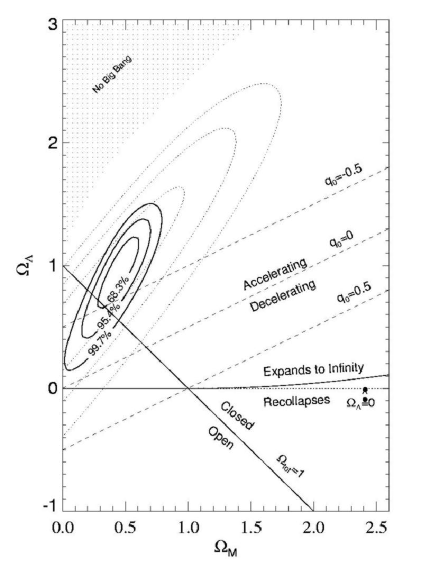
An interesting point in the evolution of the universe was the transition between deceleration and acceleration. This transition must have occurred since the early universe had to be matter dominated in order to form structure. Only recently clear evidence of the existence of this transition, or coasting point has been obtained from supernovae data [17]. The coasting point is defined as the time, or redshift, at which the deceleration parameter vanishes,
| (2.34) |
using , where
| (2.35) |
from eqn. (2.17) and using that , and we have assumed that the dark energy is parameterized by a density today, with a redshift-dependent equation of state, , not necessarily equal to .
Assuming that is constant, the coasting redshift can be determined from
| (2.36) | |||
| (2.37) |
which, in the case of a true cosmological constant, reduces to
| (2.38) |
When substituting and , one obtains , in excellent agreement with recent observations [17]. The plane can be seen in Fig. (2.1), which shows a significant improvement with respect to previous data. The best determination of the Hubble parameter was made by the Hubble Space Telescope Key Project, [24] to be km/s/Mpc, based on objects at distances up to 500 Mpc, corresponding to redshifts . In Appendix B, we provide a full list of the best fit values for the different cosmological parameters.
As a nice example, we can calculate the effect of a cosmological constant term, on our motion in the Milky Way [54]. Using the non-relativistic limit, we have:
| (2.39) |
where is the relative gravitational acceleration produced by the distribution of ordinary matter. Our solar system is moving in the Milky Way galaxy at speed roughly km/s at radius kpc. The ratio of the acceleration produced by the cosmological constant, to the total gravitational acceleration is:
| (2.40) |
a small number. The precision of celestial dynamics in the solar system is much better, but of course, the effect of a cosmological constant is much smaller, .
2.3 The Early Universe
We have already used the value of several cosmological parameters in the above calculations. An important source of information for these values comes from the Cosmic Microwave Background Radiation, or CMBR.
In table (2.1) we list the major events that took place in the history of the universe, based on the inflationary big bang model. Important for us are the end of inflation at GeV, after which the effective cosmological constant was very small, and the origin of the CMBR, since many cosmological observations that are the backbone of our theoretical models, originate from it.
| Energy of back- | Description | Time | Redshift |
| ground radiation | |||
| GeV | Planck Scale | sec | |
| GeV | Breaking of GUT | sec | |
| GeV | End of Inflation/Reheating | sec | |
| GeV | EW symm. breaking | sec | |
| 1 GeV | quark-gluon plasma condens. | sec | |
| 100 MeV | pion decay/annihilation | sec | |
| neutrino decoupling | |||
| 0.1 MeV | nucleosynthesis, | 100 sec | |
| start creation light elements | |||
| 30 keV | end nucelosynthesis | 15 min | |
| 2 eV | matter-radiation equality | 10.000 yr | 3500 |
| 0.35 eV | recombination, hydrogen-photon | 380.000 yr. | 1100 |
| decoupling, origin CMBR | |||
| Galaxy formation | years | ||
| eV | now | yr. | z=0 |
When the CMBR was discovered in 1965, its temperature was found to be 2.725 Kelvins, no matter which direction of the sky one looks at; it is the best blackbody spectrum ever measured. The CMBR appeared isotropic, indicating that the universe was very uniform at those early times.
It can be considered as the “afterglow” of the Big Bang. After the recombination of protons and electrons into neutral hydrogen, about 380,000 years after the Big Bang, the mean free path of the photons became larger than the horizon size, and the universe became transparent for the photons produced in the earlier phases of the evolution of the universe. This radiation therefore provides a snapshot of the universe at that time. The collection of points where the photons of the CMBR that are now arriving on earth had their last scattering before the universe became transparent, is called the last-scattering surface.
The universe just before recombination is a tightly coupled fluid, where photons scatter off charged particles and since they carry energy, they feel perturbations imprinted in the metric during inflation. These small perturbations propagate very similar to sound waves, a train of slight compressions and rarefactions. The compressions heated the gas, while the rarefactions cooled it, leading to a shifting pattern of hot and cold spots, the temperature anisotropies. A distinction is made between primary and secondary anisotropies, the first arise due to effects at the time of recombination, whereas the latter are generated by scattering along the line of sight. There are three basic primary perturbations, important on respectively large, intermediate, and small angular scales (see [64, 75, 76] for many details on the CMBR and its anisotropies):
-
1.
Gravitational Sachs-Wolfe. Photons from high density regions at last scattering have to climb out of potential wells, and are redshifted: , with the (perturbations in the) gravitational potential. These perturbations also cause a time dilation at the surface of last scattering, so these photons appear to come from a younger, hotter universe: , so the combined effect is .
-
2.
Intrinsic, adiabatic. Recombination occurs later in regions of higher density, causing photons coming from overly dense regions to have smaller redshift from the universal expansion, and so appear hotter: .
-
3.
Velocity, Doppler. The plasma has a certain velocity at recombination, leading to Doppler shifts in frequency and hence temperature: , with , the direction along the line of sight, and the characteristic velocity of the photons in the plasma.
Through the Cosmic Background Explorer (COBE) and, more recently, the Wilkinson Microwave Anisotropy Probe (WMAP) [18, 19] satellites, the small variations in the radiation’s temperature were detected. They are perturbations of about one part in 100,000. These tiny anisotropies are images of temperature fluctuations on the last-scattering surface and contain a wealth of cosmological information. Their angular sizes depend on their physical size at this time of last scattering, but they also depend on the geometry of the universe, through which the light has been travelling before reaching us. Maps of the temperature fluctuations are a picture of this last-scattering surface processed through the geometry and evolution of a FRW model.
During their journey through the universe, a small fraction of the CMBR photons is scattered by hot electrons in gas in clusters of galaxies. These CMBR photons gain energy as a result of this Compton scattering, which is known as the Sunyaev-Zeldovich effect, see for example [77, 78]. It is observed as a deficit of about 0.05 % of CMBR photons, as they have shifted to higher energy, with about 2 % increase. This effect can be seen as a verification of the cosmological origin of the CMBR.
A widely used code to calculate the anisotropies using linear perturbation theory is CMBFAST [79].
2.3.1 Deriving Geometric Information from CMBR Anisotropies
When looking at the CMBR, we are observing a projection of soundwaves onto the sky. A particular mode with wavelength , subtends an angle on the sky. The observed spectrum of CMB anisotropies is mapped as the magnitude of the temperature variations, versus the sizes of the hot and cold spots, and this is usually plotted through a multipole expansion in Legendre polynomials , of a correlation function . The order of the polynomial, related to the multipole moments, plays a similar role in the angular decomposition as the wavenumber does for a Fourier decomposition. Thus the value of is inversely proportional to the characteristic angular size of the wavemode it describes.
There are many good lectures on CMB physics, e.g. [64, 66, 67, 75, 80, 76] and especially the website by Hu [81].
The correlation function , is defined as follows: Let be the fractional deviation of the CMBR temperature from its mean value in the direction of a unit vector . Take two vectors and that make a fixed angle with each other: . The correlation function is then defined by averaging the product of the two ’s over the sky:
| (2.41) |
where the angle brackets denote the all-sky average over and and it is assumed that the fluctuations are Gaussian333If the -point distribution is Gaussian, it is defined by its mean vector , which is identically zero, and its covariance matrix . is a correlation function:, that because of homogeneity and isotropy only depends on [76].. In terms of Legendre polynomials:
| (2.42) |
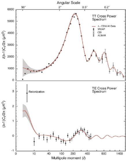
Modes caught at extrema of their oscillations become the peaks in the CMB power spectrum. They form a harmonic series based on the distance sound can travel by recombination, called the sound horizon. The first peak represents the fundamental wave of the universe, and represents the mode that compressed once inside potential wells before recombination, the second the mode that compressed and then rarefied, the third the mode that compressed then rarefied then compressed, etc. These subsequent peaks in the power spectrum represent the temperature variations caused by the overtones. All peaks have nearly the same amplitude, as predicted by inflation, except for a sharp drop-off after the third peak. The physical scale of these fluctuations is so small that they are comparable to the distance photons travel during recombination. Recombination does not occur instantaneously, the surface of last scattering has a certain thickness. In that short period during which the universe recombines, the photons bounce around the baryons and execute a random walk. If the random walk takes the photons across a wavelength of the perturbation, then the hot and cold photons mix and average out. The acoustic oscillations are exponentially damped on scales smaller than the distance photons randomly walk during recombination. See figure (2.3).
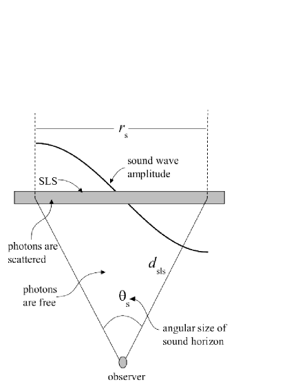
From the position of the peaks we can infer information about the geometry of the universe. In the same way as the angle subtended by say the planet Jupiter depends on both its size and its distance from us, so depend the angular sizes of the anisotropies on our distance to the surface of last scattering , from which the CMBR originated, and on what is called the “sound horizon” . The sound horizon is given by the distance sound waves could have travelled in the time before recombination, it is a fixed scale at the surface of last scattering. The angular size of the sound horizon thus becomes:
| (2.43) |
The sound horizon and the distance to the surface of last scattering, both depend on the cosmological parameters, . The distance sound can travel, from the big bang to the time of recombination is:
| (2.44) |
where are the redshift and time at recombination. See figure (2.2).
The speed of sound in the baryon-photon plasma is given by [75]:
| (2.45) |
where is the density of baryons and the speed of light.
The distance to the surface of last scattering, corresponding to its angular size, is given by what is called the angular diameter distance. It is proportional to the luminosity distance , and explicitly given by:
| (2.46) |
The location of the first peak is given by and is most sensitive to the curvature of the universe.
In [80], a very instructive calculation is presented, considering just the first peak of the spectrum, that gives a clear idea how all of this works in practise. We will review that calculation here. Taking the speed of sound (2.45) to leading order equal to and assuming that the early universe was matter dominated, we obtain for the sound horizon :
| (2.47) |
The distance to the surface of last scattering , assuming a flat universe i.e. , depends only on and . It can be derived, using that , where is the radial coordinate of the surface of last scattering. It is given by [80]:
| (2.48) |
This integral can be solved making use of a binomial expansion approximating the integrand to:
| (2.49) |
We obtain:
| (2.50) |
With our assumption of a flat universe the cosmic sum rule simply becomes . Using this, and ignoring higher order terms, we arrive at:
| (2.51) |
Together with eqn. (2.47), this gives the prediction for the first acoustic peak in a flat universe, ignoring density in radiation:
| (2.52) |
Consistent with the more accurate result, for example [82], from the MAXIMA-1 collaboration:
| (2.53) |
To summarize, the expansion in multipoles (2.3), shows that for some feature at angular size in radians, the ’s will be enhanced for a value inversely related to . For a flat universe, it shows up at lower , than it would in an open universe, see figure. The dependence of the position of the first peak on the spatial curvature can approximately be given by , with . With the high precision WMAP data, this lead to at 95% confidence level.
Much more information can be gained from the power-spectrum. A very nice place to get a feeling for the dynamics of the power spectrum is Wayne Hu’s website [81], whose discussion we also closely follow in the remainder of this section.
The effect of baryons on the CMB power spectrum is threefold:
-
1:
The more baryons there are, the more the second peak will be suppressed compared to the first. This results from the fact that the odd numbered peaks are related to how much the plasma is compressed in gravitational potential wells, whereas the even numbered peaks originate from the subsequent rarefaction of the plasma.
-
2:
With more baryons, the peaks are pushed to slightly higher multipoles , since the oscillations in the plasma will decrease.
-
3
Also at higher multipole moments, smaller angular scales, an effect can be seen, due to their effect on how sound waves are damped.
The effects of dark matter are best identified by the higher acoustic peaks, since they are sensitive to the energy density ratio of dark matter to radiation in the universe and the energy density in radiation is fairly well known. Especially the third peak is interesting. If it is higher than the second peak, this indicates dark matter dominance in the plasma, before recombination. The third peak gives the best picture for this, since in the first two peaks the self-gravity of photons and baryons is still important.
Dark matter also changes the location of the peaks, especially the first one. This is because the ratio of matter to radiation determines the age of the universe at recombination,. This in turn limits how far sound could have travelled before recombination relative to how far light travels after recombination. The spatial curvature has a similar effect, so to disentangle the two, at least three peaks have to measured.
The effect of a positive cosmological constant is a small change in how far light can travel since recombination, and hence produces a slight shift to lower multipoles.
2.3.2 Energy Density in the Universe
There is considerable evidence that most of the mass density of the universe is neither in luminous matter, nor in radiation. Since every mass gravitates, it can be detected by its gravitational influence. Most direct evidence for unseen ‘dark matter’ comes from weighing spiral galaxies. By measuring the Doppler shifts in the 21-cm line of neutral hydrogen the velocity of clouds of this gas in the disk can be mapped as a function of the distance from the center of the galaxy. One should expect this velocity to fall off as , but rather it remains constant in almost all cases, see figure (2.4).
This seems to imply that, even in the outskirts of the galaxy, the amount of mass is still growing with distance. Almost every galaxy seems to contain a ‘halo’ of dark, unseen matter, the amount of which depends on the kind of galaxy. Ranging from roughly ten times the mass seen in visible matter in spiral galaxies, to about 100 times as much in low surface brightness galaxies and dwarfs, like the Draco dwarf spheroidal galaxy, which is nearby at only 79 kpc from the Milky Way [84, 85].
This “missing mass” is a central problem in cosmology and speculations about its origin range from black holes to new species of particles, see for example [86] for a recent review. One of the most important dark matter candidates is the lightest supersymmetric particle. From the WMAP data and under certain model restrictions, an upper limit of the mass of the LSP can be derived: GeV [87].
However, there could also be a different explanation as propagated by proponents of the Modified Newtonian Dynamics (MOND) approach [88, 89, 90, 91]. MOND can perfectly describe the rotation curves of individual galaxies, but it is not without problems. Its predictions do not agree with observations of clusters of galaxies [92].
Using measurements of CMB anisotropies, statistical analysis of galaxy redshift surveys and measurements of the number density of massive galaxy clusters, it has been shown that the universe is flat to great precision and that matter, including dark matter, makes up about a quarter of the critical energy density. Combining these results with those of distant supernovae, it is inferred that about 75% of the universe is made up of dark energy. These combined experiments moreover show that the equation of state of this dark energy component is very close to -1. For more details on exactly how the different parameters are measured, see any cosmology book, like [64, 65], or more recent reviews like [66, 67].
In the past two decades or so, the picture of the contents of the universe we now have is often abbreviated as CDM. A universe, with dominant cosmological constant, or dark energy and Cold Dark Matter.
2.4 Evolution of the Universe
We will now consider universes dominated by matter and vacuum energy, as given in the previous section. As discussed, a positive cosmological constant tends to accelerate the universal expansion, while ordinary matter and a negative cosmological constant tend to decelerate it. The relative contributions to the energy density of the universe scale like:
| (2.54) |
From the Friedmann equations:
| (2.55) |
we can immediately infer that, if , the universe will always recollapse to a big crunch, either because the matter density is sufficiently high or because eventually the negative cosmological constant will dominate. For the universe will expand forever, unless there is sufficient matter to cause a recollapse before becomes dynamically important. For on the hand the universe will expand forever if or will recollapse if . To identify these boundaries properly, let us have look again at the equation for the time-dependent Hubble parameter:
| (2.56) |
with dimensionless scalefactor and writing from the cosmic sum rule, we have:
| (2.57) |
Now we have to find solutions for which the left-hand-side vanishes, since these define the turning points in the expansion. There are four conditions, see for example [93, 64, 66, 67]:
-
1:
As already stated before, negative always implies recollapse.
-
2:
If is positive and , the model always expands to infinity.
-
3:
If , recollapse is only avoided if exceeds a critical value:
(2.58) -
4:
Conversely, if the cosmological constant is sufficiently large compared to the matter density, there was, no initial singularity, no Big Bang. Its early history consisted of a period of gradually slowing contraction to a minimum radius before beginning its current expansion; it underwent a bounce. The criterion for there to have been no singularity in the past is
(2.59) where “coss” represents when , and when .
If the universe lies exactly on the critical line, the bounce is at infinitely early times. Models that almost satisfy the critical relation are called loitering models, since they spent a long time close to constant scale factor. However, these bounce models can be ruled out quite strongly, since the same cubic equations also give a relation for the maximum possible redshift [64]:
(2.60) With as low as 0.1, a bounce is ruled out once objects are seen at redshift . Since galaxies have even been observed at , these universes are indeed ruled out.
This defines the boundaries between the different regions, summarized in the -plane (2.1).
The behavior of the universe can also be seen by referring to our previous expression for the deceleration parameter :
| (2.61) |
Uniform expansion () corresponds to the line . Points above this line correspond to universes that are accelerating today, while those below correspond to decelerating universes, in particular the old cosmological model of Einstein-de Sitter (EdS), with . Since 1998, all the data from Supernovae of type Ia appear above this line, many standard deviations away from EdS universes. Nevertheless, sometimes it is argued, that the EdS universe is a sound alternative to the concordance model, and that it is in better agreement with the low quadrupole in the CMBR [94]. In such a universe, the Hubble constant would be significantly lower, approximately 46 km/s/Mpc, the SNIa results would have to be discarded, for some systematical error for example, and one would have to introduce another source of dark matter, to suppress power on small scales. This seems a very contrived conspiracy of effects, and has not many proponents.
The line corresponds with a flat universe, . Points to the right of this line correspond to closed universes, while those to the left correspond to open ones. In the last few years we have mounting evidence that the universe is spatially flat (in fact Euclidean).
2.5 Precision cosmology in recent and upcoming experiments
In the past two decades or so cosmology has really grown as a very interesting field of study. Especially observational cosmology has made astonishing progress producing the first maps of the cosmos and of course showing the acceleration of the expansion of the universe. In this section we will review the supernovae experiments, since these have been so important for the discovery of an accelerating universe, and briefly discuss the Pioneer anomaly, as it has been used to argue for deviations of general relativity.
2.5.1 Supernovae Type Ia
From the end of the 1990’s, two independent teams, the “Supernova Cosmology project”, led by Perlmutter of Lawrence Berkeley Laboratory and “The High-Z Supernova Search Team”, led by Schmidt of Mt. Stromlo and Siding Observatories, have used the apparent brightness of supernovae in order to study the speed of the expansion of the universe. Both teams found that these supernovae look fainter than expected. With the assumption, based on CMBR experiments that the universe is flat, this could be the result of a cosmological constant. This can be easily seen from the expressions for the luminosity distance , which in a matter dominated universe take the form:
| (2.62) |
whereas in a cosmological constant dominated universe :
| (2.63) |
This shows that at given redshift , the luminosity distance is larger for a universe where the cosmological constant dominates, and hence, a given object, at a fixed redshift, will appear fainter.
For objects close by there is a linear relation between these two quantities and the fixed ratio of the two is known as Hubble’s constant. For objects farther away though, deviations from this linear dependence can be expected, either because the speed of the expansion has changed over time, or as a result of spacetime curvature. Therefore, to track down the history of the expansion one has to find the distance-redshift relation of objects located very far away. In Hubble’s day, distances were determined by assuming that all galaxies have the same intrinsic brightness. So the fainter a galaxy really appeared, the further away from us it is located and vice versa. This is a very crude way of determining distances since different galaxies can have very different properties, and therefore different intrinsic brightness. Moreover, when looking at galaxies located far away, evolutionary effects play an important role since light takes so long to travel to us. We then view these galaxies as they were billions of years ago, in their youth, and their intrinsic brightness could be very different from the more mature ones, seen closer at home.
Distances are measured in terms of the “distance modulus” , where is the apparent magnitude of the source, and its absolute magnitude. This distance modulus is related to the luminosity distance:
| (2.64) |
A very useful relation, if you know the absolute magnitude, which is notoriously hard to infer for a distant object. It is very difficult to disentangle evolutionary changes from the effects of the expansion, so astronomers have been looking for objects called “standard candles”, whose intrinsic brightness, and therefore distance, can be determined more unambiguously. The best candidate for this task is a particular type of supernovae (SNe). Supernovae, extremely bright explosions of a dead star, about 10 billion times as luminous as our sun, are among the most violent phenomena in our universe. They come in two main classes [95] called Type II for supernovae whose optical spectra exhibit hydrogen lines, while hydrogen deficient SNe are designated Type I. These SNe Type I are further subdivided according to the detailed appearance of their early-time spectrum. SNe Ia are characterized by strong absorption near 6150 , corresponding to SiII. SNe Ib lack this feature but instead show prominent HeI lines. SNe Ic finally have neither SiII nor HeI lines. In practise there is often little distinction between the latter two types and they are most commonly designated as Type Ib/c.
For the Type II SNe, four subclasses exist based on the shape of optical light curves, see [96] for the details. For our purposes the Type Ia are the only relevant ones.
There are two physical mechanisms that produce supernovae: thermonuclear (the SNe Ia are the only ones of this type) and the more common core collapse of a massive star. This last type occurs when a massive red supergiant becomes old and produces more and more metals in its core. Stars never fuse elements heavier than iron, since this would cost energy, rather than produce it. Thus iron piles up until this iron core reaches the Chandrasekhar mass, which is about 1.4 solar masses. This is the critical mass below which electron degeneracy pressure can stand up to the gravitational pressure, but above this mass, no such equilibrium is possible and the core collapses. At the extreme high pressure in the core protons and electrons are smashed together to form neutrons and neutrinos, while at the same time the outer layers crash into the core and rebound, sending shockwaves outward. These two effects together cause the entire star outside the core to be blown apart in a huge explosion, a Type II supernova! What is left behind of the core will be either a neutron star or, if it is heavy enough, a black hole.
SNe Ia on the other hand originate from a white dwarf star that accretes matter from another star orbiting nearby, until the Chandrasekhar limit is reached. This happens for example in a binary system, when a white dwarf can start slurping up matter from a main sequence star that expands into a giant or supergiant. When the critical mass is reached, the star is no longer stable against gravitational collapse: the radius decreases, while the density and temperature increase. The fusion of carbon and oxygen into iron now occurs very rapidly, converting the star to a fusion bomb until a thermonuclear firestorm ignites. The dwarf star gets completely blown apart, spewing out material at about 10,000 kilometers per second. The amount of energy released in this cosmic showpiece is about joules, as much as the Sun has radiated away during its entire lifetime. The glow of this fireball takes about three weeks to reach its maximum brightness and then declines over a period of months. The spectrum contains no hydrogen or helium lines, since the dwarf that is blown apart consists of carbon and oxygen. Yet it does show silicon lines, since that is one of the products of fusing carbon and oxygen.
In a typical galaxy such a SNe 1a lights up every 300 years or so. In our own Milky Way therefore, it is a rare celestial event. The last supernova in our galaxy was seen in 1604 by Kepler. However, if you monitor a few thousand galaxies, you can expect to witness about one type 1a supernova every month. There are actually so many galaxies in the universe that a supernova bright enough to study erupts every few seconds! You only have to find them. Catching a supernova at its peak brightness however is not so easy as their occurrence cannot be predicted and observing time at the worlds largest telescopes therefore cannot be scheduled in advance. Moreover, these type 1a also vary in their brilliance, but brighter explosions last somewhat longer than fainter ones. Therefore, they must be very carefully observed multiple times during the first weeks, to monitor how long they last. This way their intrinsic brightness can be deduced to within 12 percent (absolute magnitude ). In terms of redshift, supernovae with redshifts as high as have been observed. This corresponds to a time when the universe was about one-third its current age444That is, for a Hubble constant km/s/Mpc leading to a current age of the universe of about 14 billion years..
The supernova results show that although the universe is undergoing accelerated expansion now, this has not always been the case. Up until about 5 billion years ago, the universe was matter dominated and decelerating. The change between these two phases occurred at about . For a recent review of type Ia supernovae in cosmology, see [97].
2.5.2 Pioneer Anomaly
Another phenomenon that perhaps should be explained as a deviation of GR originates from within our solar system and has become known as the Pioneer anomaly. The two space probes Pioneer 10 and 11 were launched in the beginning of the seventies to do measurements on Jupiter and Saturn along the outskirts of our solar system. At distances from the sun between 20 and 70 astronomical units (AU), the Doppler data have shown a deviation from calculations based on GR. Analysis indicated a small, constant Doppler blue shift drift of order Hz/s. After accounting for systematics, this may be interpreted as an unexplained, constant acceleration directed towards the sun with a roughly constant amplitude: , or perhaps a time acceleration of , see e.g. [98] for a recent review and many references.
Various mechanisms have been considered to explain this acceleration, but so far no satisfactory scenario has been put forward see [99, 100, 101, 102] and references therein. The inability of conventional physics to explain the anomaly, has triggered a growing number of new theoretical explanations. One popular explanation was based on a Yukawa modification of Newton’s law, but it quickly became clear that explaining the Pioneer anomaly in terms of a long-range Yukawa correction, would also lead to very large deviations from Kepler’s law or of the precession of perihelions which obviously have not been observed [103, 104]. Other proposals suggest that we see here effects due to dark matter. If dark matter should be held accountable for the anomalous acceleration, it would have to be distributed in the form of a disk in the outer solar system, with a constant density of . The acceleration, due to any drag force from an interplanetary medium ia:
| (2.65) |
with the effective reflection/absorption/transmission coefficient of the spacecraft surface, the density of the medium, the effective relative velocity of the craft to the medium, the spacecraft’s cross-section, and its mass. The mass of the spacecraft is 241 kg, its cross-section about and its speed nowadays roughly 12 km/s. A constant density of would therefore explain the Pioneer Anomaly. This would be in correspondence with bounds on dark matter within the outer regions of our solar system of about , [105]. A spherical halo of a degenerate gas of massive neutrinos with keV, around the sun [105] and mirror matter [106, 107] have been suggested.
Another proposal suggests that the modified inertia interpretation of gravity called ‘Modified Newtonian Dynamics’ or MOND for short, gives a correct explanation [108, 109]. Also certain braneworld scenarios [110] presumably can explain the observed effect, with a right adjustment of parameters for the potential of a scalar field.
Chapter 3 Type I: Symmetry Mechanism
One can set the cosmological constant to any value one likes, by simply adjusting the value of the bare cosmological constant. No further explanation then is needed. This fine-tuning has to be precise to better than at least 55 decimal places (assuming some TeV scale cut-off), but that is of course not a practical problem. Since we feel some important aspects of gravity are still lacking in our understanding and nothing can be learned from this ‘mechanism’, we do not consider this to be a physical solution. However, it is a possibility that we can not totally ignore and it is mentioned here just for sake of completeness.
A natural way to understand the smallness of a physical parameter is in terms of a symmetry that altogether forbids any such term to appear. This is also often referred to as ‘naturalness’: a theory obeys naturalness only if all of its small parameters would lead to an enhancement of its exact symmetry group when replaced by zero. Nature has provided us with several examples of this. Often mentioned in this respect is the example of the mass of the photon. The upper bound on the mass (squared) of the photon from terrestrial measurements of the magnetic field yields:
| (3.1) |
The most stringent estimates on nowadays give:
| (3.2) |
We ‘know’ the mass of the photon to be in principle exactly equal to , because due to the gauge symmetry of QED, the photon has only two physical degrees of freedom (helicities). In combination with Lorentz invariance this sets the mass equal to zero. A photon with only two transverse degrees of freedom can only get a mass if Lorentz invariance is broken. This suggests that there might also be a symmetry acting to keep the effective cosmological constant an extra 34 orders of magnitude smaller.
A perhaps better example to understand the smallness of a mass is chiral symmetry. If chiral symmetry were an exact invariance of Nature, quark masses and in particular masses for the pseudoscalar mesons would be zero. The spontaneous breakdown of chiral symmetry would imply pseudoscalar Goldstone bosons, which would be massless in the limit of zero quark mass. The octet would be the obvious candidate and indeed the pion is by far the lightest of the mesons. Making this identification of the pion being the pseudo-Goldstone boson associated with spontaneous breaking of chiral symmetry, we can understand why the pion-mass is so much smaller than for example the proton mass.
3.1 Supersymmetry
One symmetry with this desirable feature for the energy density of the ground state, is supersymmetry, or SUSY for short. Contributions to the energy density of the vacuum in field theory coming from fields with spin are (eqn. (1.22)):
| (3.3) | |||||
so if for each mass there are an equal number of fermionic and bosonic degrees of freedom, the net contribution to would be zero. Supersymmetry posits exactly such a symmetry, and hence realizes elegantly that the energy density of the ground state is zero.
The spin- generators of the supersymmetry transformations, called supercharges are denoted by and they satisfy anticommutation relations:
| (3.4) |
where and are two-component spin indices, are the Pauli-matrices, and is the energy-momentum operator. Summing over and , we find the Hamiltonian:
| (3.5) |
where is the energy operator. Matrix elements of can be written as:
| (3.6) |
with
| (3.7) |
Thus in a supersymmetric theory, the energy of any non-vacuum state in a positive definite Hilbert space, is positive definite. Moreover, if supersymmetry is unbroken, the vacuum state satisfies for all ) and we see that this state has vanishing energy:
| (3.8) |
This includes all quantum corrections and would nicely explain a vanishing vacuum energy.
This same result can also be obtained by looking at the potential. The scalar field potential in supersymmetric theories takes on a special form. Scalar fields must be complex, to match the degrees of freedom coming from the fermions, and the potential is derived from a function, called the superpotential which is necessarily holomorphic (written in terms of and not its complex conjugate ). In the simple Wess-Zumino models of just spin- and spin- fields, for example, the scalar potential is given by:
| (3.9) |
where . Supersymmetry will be unbroken only for values of such that , implying that takes it minimum value . Quantum effects do not change this conclusion, since the boson-fermion symmetry ensures that boson-loops are cancelled against fermion-loops.
So if supersymmetry were an exact symmetry of nature, there would be bosons and superpartner-fermions with the same mass and the vacuum state of this theory would have zero energy. However, these supersymmetric partners of the Standard Model particles have not been found, so SUSY has to be broken at least at the TeV scale, which again induces a large vacuum energy.
Besides, we still have the freedom to add any constant to the Lagrangian, thereby changing the value of the effective cosmological constant. In order to discuss the cosmological constant problem properly, we need to bring gravity into the picture. This implies making the supersymmetry transformations local, leading to the theory of supergravity or SUGRA for short. In such a theory the value of the effective cosmological constant is given by the expectation value of the potential.
3.1.1 No-Scale SUGRA
In exact SUGRA the lowest energy state of the theory, generically has negative energy density111This negative energy density can also be forbidden by postulating an unbroken R-symmetry.. Or, in other words, the vacuum of supergravity is AdS. This has inspired many to consider so-called no-scale supergravity models in which supersymmetry breaking contributes precisely the amount of positive vacuum energy to make the net result equal to zero. See [40] or supersymmetry textbooks such as [111] for excellent reviews. In this section we closely follow [111].
The pure supergravity (SUGRA) Lagrangian, that is without interactions, is:
| (3.10) |
where is the Einstein-Hilbert term, is the Rarita-Schwinger Lagrangian describing the free gravitino and , a pseudoscalar, a scalar and an axial vector, are auxiliary fields to match the on- and off-shell fermionic and bosonic degrees of freedom. The full Lagrangian is characterized by two arbitrary functions of the scalar fields (in the presence of gravity, renormalizability is lost anyway, so there is no reason to require only low-order polynomials in ): a real function , called the Kähler potential and an analytic function , where Latin indices are gauge indices. These functions determine the general forms allowed for the kinetic energy terms of the scalar fields and of the gauge fields , respectively. Some of the terms from the full Lagrangian that are important for now are:
| (3.11) | |||||
in which the gravitational coupling has been set equal to one and:
| (3.12) |
The scalar kinetic energy term shows that plays the role of the metric in the space spanned by the scalar fields. A metric of this form is referred to as a Kähler metric and is called the Kähler potential. In the absence of gravity and . The function is invariant under transformations of the gauge group, whereas transforms as a symmetric product of two adjoint representations of that group.
The Lagrangian contains a scalar potential which generally consists of so-called D-terms and F-terms. The D-terms arise from removing the auxiliary scalar fields contributing to the gauge multiplets, and the F-terms from removing the auxiliary scalar fields of the chiral matter multiplets. With denoting the superpotential, one finds:
| (3.13) |
where we now must include the Kähler metric. This gives the first term of the scalar potential:
| (3.14) |
In case of supergravity, there is an additional contribution form eliminating the auxiliary scalar field terms in (3.10) and this yields the second term of (3.14). The negative sign has important consequences. The factor arises from the Weyl rescaling of the fields required to bring the first term in (3.11) into the canonical Einstein form. This rescaling also implies a redefinition of the fermion fields and hence the factor in the last term as well. Owing to this term, when local SUSY is spontaneously broken the gravitino acquires a mass:
| (3.15) |
where then has to evaluated ar the minimum of the potential.
In general the Kähler potential has to satisfy certain conditions for the theory to be well defined, for example , in order for the kinetic terms of the scalar fields to have the correct sign. A special choice is:
| (3.16) |
with the superpotential. This choice gives and hence the minimal kinetic terms as in global SUSY. The scalar potential becomes:
| (3.17) |
Now we come to the important point. There is an elegant way of guaranteeing a flat potential, with after supersymmetry breaking, by using a nontrivial form of the Kähler potential . So far we have used the minimal form of which lead to the above scalar potential. For a single scalar field :
| (3.18) | |||||
A flat potential with is obtained if the expression in brackets vanishes for all , which happens if:
| (3.19) |
and one obtains a gravitino mass:
| (3.20) |
which, as required, is not fixed by the minimization of . Thus provided one chooses a suitable, nontrivial form for the Kähler potential , it is possible to obtain a zero CC and to leave the gravitino mass undetermined, just fixed dynamically through non-gravitational radiative corrections. The minimum of the effective potential occurs at:
| (3.21) |
where in this case, after including the observable sector and soft symmetry-breaking terms, . Such a mass is ruled out cosmologically, see e.g. [112], and so other models with the same ideas have been constructed that allow a very small mass for the gravitino, also by choosing a specific Kähler potential, see [113].
That these constructions are possible is quite interesting and in the past there has been some excitement when superstring theory seemed to implicate precisely the kinds of Kähler potential as needed here, see for example [114]. However, that is not enough, these simple structures are not expected to hold beyond zeroth order in perturbation theory.
SUGRA seems to be a special case; its symmetries implicitly forbid a CC term, see [115]. However, also here, the vanishing of the vacuum energy is a purely classical phenomenon, which is spoiled by quantum corrections after supersymmetry breaking.
3.1.2 Unbroken SUSY
To paraphrase Witten [116]: “Within the known structure of physics, supergravity in four dimensions leads to a dichotomy: either the symmetry is unbroken and bosons and fermions are degenerate, or the symmetry is broken and the vanishing of the CC is difficult to understand”. However, as he also argues in the same article, in dimensions, this unsatisfactory dichotomy does not arise: SUSY can explain the vanishing of the CC without leading to equality of boson and fermion masses, see also [117].
The argument here is that in order to have equal masses for the bosons and fermions in the same supermultiplet one has to have unbroken global supercharges. These are determined by spinor fields which are covariantly constant at infinity. The supercurrents from which the supercharges are derived are generically not conserved in the usual sense, but covariantly conserved: . However, in the presence of a covariantly constant spinor (), the conserved current can be constructed and therefore, a globally conserved supercharge:
| (3.22) |
But in a dimensional spacetime any state of non-zero energy produces a geometry that is asymptotically conical at infinity (see also [118]). The spinor fields are then no longer covariantly constant at infinity [119] and so even when supersymmetry applies to the vacuum and ensures the vanishing of the vacuum energy, it does not apply to the excited states. Explicit examples have been constructed in [120, 121, 122, 123]. Two further ideas in this direction, one in and one in are [124, 125], however the latter later turned out to be internally inconsistent [126].
In any case, what is very important is to make the statement of “breaking of supersymmetry” more precise. As is clear, we do not observe mass degeneracies between fermions and bosons, therefore supersymmetry, even if it were a good symmetry at high energies between excited states, is broken at lower energies. However, and this is the point, as the example of Witten shows, the issue of whether we do or do not live in a supersymmetric vacuum state is another question. In some scenarios it is possible to have a supersymmetric vacuum state, without supersymmetric excited states. This really seems to be what we are looking for. The observations of a small or even zero CC could point in the direction of a (nearly) supersymmetric vacuum state.
Obviously the question remains how this scenario and the absence nevertheless of a supersymmetric spectrum can be incorporated in 4 dimensions, where generically spacetime is asymptotically flat around matter sources.
3.1.3 Non-SUSY String Models
It has been suggested that the cosmological constant might vanish in certain string models [127, 128] due to an equality between the number of boson and fermion mass states, despite the fact that supersymmetry is broken. The one-loop contribution to the cosmological constant therefore vanishes trivially, but it is claimed that even higher order corrections would not spoil this cancellation.
These ideas have been challenged in [129, 130], where it was argued that higher loop corrections would indeed spoil the tree level results. The most important drawbacks however for this proposed scenario, is that the non-Abelian gauge sector, was always supersymmetric [131, 132, 133]. These approaches thus do not lead to viable models.
3.2 Scale Invariance, e.g. Conformal Symmetry
Another interesting symmetry with respect to the cosmological constant problem is conformal symmetry, . Massless particles are symmetric under a bigger group than just the Lorentz group, namely, the conformal group. This group does not act as symmetries of Minkowski spacetime, but under a (mathematically useful) completion, the “conformal compactification of Minkowski space”. This group is 15-dimensional and corresponds to , or if fermions are present, the covering group . Conformal symmetry forbids any term that sets a length scale, so a cosmological constant is not allowed, and indeed also particle masses necessarily have to vanish.
General coordinate transformations and scale invariance, i.e. , are incompatible in general relativity. The term in the Einstein-Hilbert action is the only quantity that can be constructed from the metric tensor and its first and second derivatives only, that is invariant under general coordinate transformations. But this term is not even invariant under a global scale transformation for which is constant. transforms with Weyl weight and with weight . There are two ways to proceed to construct a scale invariant action: introducing a new scalar field [134, 135], that transforms with weight , giving rise to so-called scalar-tensor theories, or consider Lagrangians that are quadratic in the curvature scalar. We consider the second. See for example [136, 137] for some resent studies and many references.
Gravity can be formulated under this bigger group, leading to “Conformal gravity”, defined in terms of the Weyl tensor, which corresponds to the traceless part of the Riemann tensor:
| (3.23) | |||||
where is the conformal Weyl tensor, and is a dimensionless gravitational coupling constant. Thus the Lagrangian is quadratic in the curvature scalar and generates field equations that are fourth-order differential equations. Based on the successes of gauge theories with spontaneously broken symmetries and the generation of the Fermi-constant, one may suggest to also dynamically induce the Einstein action with its Newtonian constant as a macroscopic limit of a microscopical conformal theory. This approach has been studied especially by Mannheim and Kazanas, see [138, 139, 140, 141, 142, 143] to solve the CC problem.
These fourth-order equations reduce to a fourth-order Poisson equation:
| (3.24) |
where and the source is given by:
| (3.25) |
For a static, spherically symmetric source, conformal symmetry allows one to put and the exterior solution to (3.24) can be written [143]:
| (3.26) |
Assuming that the quadratic term is negligible at solar system distance scales, the non-relativistic potential can be written:
| (3.27) |
However, for a spherical source (3.24) can be completely integrated to yield:
| (3.28) |
Compared to the standard second-order equations:
| (3.29) |
we see that the fourth-order equations contain the Newtonian potential in its solution, but in addition also a linear potential term that one would like to see dominate over Newtonian gravity only at large distances. The factors and in for example (3.27) are given by:
| (3.30) |
Even if this would be correct, modifying gravity only at large distances cannot solve the cosmological constant problem. The (nearly) vanishing of the vacuum energy and consequently flat and relatively slowly expanding spacetime is a puzzle already at distance scales of say a meter. We could expect deviations of GR at galactic scales, avoiding the need for dark matter, but at solar system scales GR in principle works perfectly fine. It seems hard to improve on this with conformal symmetry, since the world simply is not scale invariant.
We also identified a more serious problem with the scenario of Mannheim and Kazanas described above. In order for the linear term not to dominate already at say solar system distances, the coefficient has to be chosen very small. Not only would this introduce a new kind of fine-tuning, it is also simply not allowed to choose these coefficients at will. The linear term will always dominate over the Newtonian -term, in contradiction with the perfect agreement of GR at these scales. See also [144] who raised the same objection.
This scenario therefore does not work.
3.2.1 as Integration Constant
Another option is to reformulate the action principle in such a way that a scale dependent quantity like the scalar curvature, remains undetermined by the field equations themselves. These are the so-called ‘unimodular’ theories of gravity, see e.g. [145, 146]. Note that although the action is not globally scale invariant, Einstein’s equations in the absence of matter and with vanishing cosmological constant is. The dynamical equations of pure gravity in other words, are invariant with respect to global scale transformations, and since we have that , they are scale-free, i.e. they contain no intrinsic length scale.
There is a way to keep the scale dependence undetermined also after including matter which also generates a cosmological constant term. This well-known procedure [147, 148] starts by imposing a constraint on the fluctuations in , such that the determinant of the metric is fixed:
| (3.31) |
where is a scalar density of weight . The resulting field equations are:
| (3.32) |
The covariant derivative still vanishes and from this one obtains:
| (3.33) |
where now appears as an integration constant and the factor of has been chosen for convenience since substituting this back we recover the normal Einstein equations with cosmological constant.
Recently, some arguments have been put forward in which a unimodular theory is supposed to originate more naturally as a result of ‘the quantum microstructure of spacetime being capable of readjusting itself, soaking up any vacuum energy’, see [149, 38, 150].
Obviously this does not solve much, nor does it provide a better understanding of the cosmological constant. The restriction (3.31) on the variation of the metric has no deeper motivation and the value of the integration constant has to be inserted by hand in order to arrive at the correct value.
Besides, sometimes it is concluded that there are two inequivalent Einstein equations for gravity, describing two theories that are only equivalent classically, but not quantum mechanically. The group of canonical transformations is much larger than that of unitary transformations in Hilbert space, forcing one to quantize in “preferred” coordinates. We do not agree with this point of view. The constraint just reflects a choice of coordinates, a certain gauge.
This issue is closely related to the question of the measure of the quantum gravity functional integral (see discussions by B.S. DeWitt [151, 152], ’t Hooft [153] and [154]): Is the integration variable , or some other function of the metric? The differences in the amplitudes for these theories all appear in the one-loop diagrams, in the form of quartically divergent momentum-independent ghost loops. These all disappear after renormalization and therefore the theories are indistinguishable physically.
3.3 Holography
Gravitational holography [155, 156] limits the number of states accessible to a system. The entropy of a region generally grows with its covering area (in Planck units) rather than with its volume, implying that the dimension of the Hilbert space, i.e. the number of degrees of freedom describing a region, is finite and much smaller than expected from quantum field theory. Considering an infinite contribution to the vacuum energy is not correct because states are counted that do not exist in a holographic theory of gravity.
It is a symmetry principle since there is a projection from states in the bulk-volume, to states on the covering surface.
In [157, 158] it is noted that in effective field theory in a box of size with UV cutoff the entropy scales extensively, as . A free Weyl fermion on a lattice of size and spacing has states and entropy222For bosons the number of states is not limited by a lattice cutoff alone, so in this argument one has to limit oneself to fermions. For bosons there are an infinite number of states, in contradiction to the conjecture of the Holographic Principle. . The corresponding entropy density then is . In dimensions quantum corrections to the vacuum energy are therefore of order:
| (3.34) |
since both and are dominated by ultraviolet modes, (see also [159]). Thus finite implies finite corrections to .
Using a cutoff , is the maximum energy for a system of size . States with , with the Schwarzschild radius, or (in Planckian units) have collapsed into a black-hole. If one simply requires that no state in the Hilbert space exists with , then a relation between the size of the region, providing an IR cutoff, and the UV cutoff can be derived, in natural units:
| (3.35) |
This corresponds to the assumption that the effective theory describes all states of the system, except those that have already collapsed to a black hole.
Under these conditions entropy grows no faster than , with the area. If these black hole states give no contribution to , we obtain:
| (3.36) |
In [157] this same scaling was obtained by assuming that as usual, but that the delocalized states have typical Heisenberg energy :
| (3.37) |
Plugging in for the observed size of the universe today the quantum corrections are only of order .
However, this does not yield the correct equation of state, [159]. During matter dominated epochs, to which WMAP and supernova measurements are sensitive, the horizon size grows as the RW-scale factor, , so the above arguments imply:
| (3.38) |
or, at largest scales, since . The data on the other hand give (95% CL) [19]. In [157, 158] is at all times comparable to the radiation + matter energy density, which is also argued to give problems for structure formation [160].
Holography-based scenarios thus naively lead to a cosmological constant that is far less constant than what the data require. This makes a connection between holography and dark energy a lot harder to understand333In [161] in a different context a similar relation between the CC and the volume of the universe is derived, thus suffering from the same drawbacks..
More recently however, another proposal was made [162] where instead is taken to be proportional to the size of the future event horizon:
| (3.39) |
This describes the size of the largest portion of the universe that any observer will see. This could be a reasonable IR cutoff. It is argued that in this case the equation of state parameter can be close enough to to agree with the data. This relation is rather ad hoc chosen, and its deeper meaning, if any, still has to be discovered.
A very recent paper studying the implications of the holographic principle for the cosmological constant problem is [163], in which it is argued that holography makes a tiny value for the cosmological constant ‘natural’ in a large universe. This is however a rather empty statement, since a large (observable) universe necessarily must have a tiny value for the cosmological constant. In other words, if the universe is large the effective cosmological constant must be small, and no holographic arguments are needed for that.
3.3.1 Conceptual Issues in de Sitter Space
Another reason to discuss holography in the context of the cosmological constant problem lies in trying to reconcile string theory with the apparent observation of living in a de Sitter spacetime, see [164] for a construction of de Sitter vacua in string theory. The discussion centers around the semi-classical result that de Sitter space has a finite entropy, inversely related to the cosmological constant. As discussed in section (1.5), the entropy is given by:
| (3.40) |
with the area of the horizon. It seems natural to interpret this entropy as the number of quantum states necessary to describe a de Sitter universe [39, 165]. This interpretation is common in thermodynamics, and is also given for the entropy of a black hole. Another motivation for this interpretation arises from the fact that the classical phase space of general relativity with asymptotic de Sitter boundary conditions, both in the past and in the future, is compact. A compact phase space yields a finite dimensional Hilbert space when quantized. Thus one may reason that de Sitter space, or better, asymptotic de Sitter space, since the metric fluctuates, should be described by a theory with a finite number of independent quantum states and that a theory of quantum gravity should be constructed with a Hilbert space of finite dimension in terms of which the entropy is given by:
| (3.41) |
In this reasoning a cosmological constant should be understood as a direct consequence of the finite number of states in the Hilbert space describing the world. Ergo, the larger the cosmological constant, the smaller the Hilbert space:
| (3.42) |
Banks [39] therefore argues that the cosmological constant should not be viewed as a derived, calculable quantity, but instead as a fundamental input parameter. In [166] this reasoning is criticized. In any case, finiteness of entropy and Hilbert space leads to several conceptual difficulties.
One is that only compact groups can have non-trivial finite-dimensional unitary representations, but the de Sitter group is non-compact. Therefore, it has been claimed that either de Sitter space has no holographic dual [35], which would make it impossible to have an analog of the successful AdS/CFT dual for de Sitter space, or that in fact the correct symmetry group is not the standard de Sitter group [34]. However, whether these claims hold in the future is unclear, and ways out of this conundrum have been proposed, for example [167]. See also [168, 37] in which a holographic dS/CFT correspondence is formulated, in apparent contradiction to the above claim, since the CFT Hilbert space is in principle infinite dimensional. It appears to be an unsettled question whether this leads to consistent theories, especially since no explicit example is known, in which a dS/CFT emerges directly from string theory, see also the discussion in [36].
Another issue, as hinted on in the first chapter of this thesis, arguments have been made that the standard Einstein-Hilbert action with cosmological constant cannot be quantized for general values of and , but that it must be derived from a more fundamental theory, which determines these values [34]. The reasoning behind this statement is that although the Hilbert space of quantum gravity in de Sitter space has finite dimension, it is infinite dimensional perturbatively. Perturbation theory is an expansion in powers , in four dimensions. In the limit , diverges exponentially, if (3.41) holds. In fact, will be non-trivial function of , yet it has to take integer values, whereas the latter can vary continuously.
However, it not immediately clear to which states the number refers to. Because of the appearance of negative absolute temperatures, it has been argued in [169] that instead of the usual thermodynamic relation:
| (3.43) |
the equation on the right should be used to compute the de Sitter temperature. The idea behind this is that the de Sitter entropy should perhaps be ascribed to states behind the horizon, which cannot be observed.
Finally, another difficulty in de Sitter space has to to with formulating ordinary quantum field theory. In quantum field theory, in order to set up an S-matrix, one has to define incoming and outgoing states, and these are only properly defined at spatial infinity. De Sitter space however, is compact, there is no notion of spatial infinity, only of temporal past and future asymptotic regions. Matrix elements constructed this way are therefore no measurable quantities. Note that also the conventional formulation of string theory is based on the existence of an S-matrix.
Another quantum field theory aspect is that there appear to be instabilities in de Sitter space, for example in case of a scalar field, but perhaps also in pure gravity. These issues are discussed in chapter 5 and 6.
Much more needs to be understood about these issues to judge their validity and possible impact on the cosmological constant problem. It is clear however, that the measurements indicating an accelerating universe and a dark energy equation of state , have much more far-reaching consequences than ‘just’ the ordinary cosmological constant problem. In other words, a solution to the cosmological constant problem, especially if not by some symmetry, seems to have very deep implications for a broad range of theoretical physics.
3.4 “Symmetry” between Sub- and Super-Planckian Degrees of Freedom
This rather speculative reasoning originates from a comparison with condensed matter physics and is due to Volovik, see for example [170, 171, 172, 173, 174, 175, 176, 177]. The vacuum energy of superfluid 4Helium, calculated from an effective theory containing phonons as elementary bosonic particles and no fermions is:
| (3.44) |
with the determinant of the acoustic metric, since is now the speed of sound, and , with the interatomic distance, which plays the role of the Planck length. However, in the condensed matter case, the full theory exists: a second quantized Hamiltonian describing a collection of a macroscopic number of structureless 4Helium bosons or 3Helium fermions, in which the chemical potential acts as a Lagrange multiplier to ensure conservation of the number of atoms:
| (3.45) | |||||
Using this Hamiltonian to calculate the energy density of the ground state we get:
| (3.46) |
An overall shift of the energy in is cancelled in a shift of the chemical potential. Exact calculation shows that not only the low energy degrees of freedom from the effective theory, the phonons, but also the higher energy, “trans-Planckian” degrees of freedom have to be taken into account.
Besides, for a liquid of identical particles at temperature in a volume in equilibrium, the relation between the energy and pressure is given by the Gibbs-Duhem equation:
| (3.47) |
Therefore at the energy density of the ground state becomes:
| (3.48) |
the same equation of state as for the vacuum state in GR. Using just thermodynamic arguments, it is argued that in the infinite volume, zero temperature limit, this gives exactly zero vacuum energy density as long as there are no external forces, i.e. no pressure acting on the quantum liquid. And assuming there is no matter, no curvature and no boundaries which could give rise to a Casimir effect [171].
The conclusion therefore is that, if these thermodynamic arguments are also valid in a gravitational background for the universe as a whole and up to extremely high energies, one would expect a perfect cancellation between sub- and super-Planckian degrees of freedom contributing to the vacuum energy, resulting in zero cosmological constant.
Moreover, it is also argued that a non-zero cosmological constant arises from perturbations of the vacuum at non-zero temperature. The vacuum energy density would be proportional to the matter energy density, solving the coincidence problem as well.
A similar result is obtained by [178]. In their formulation the world is like a crystal. The atoms of the crystal are in thermal equilibrium and exhibit therefore zero pressure, making the cosmological constant equal to zero.
Both approaches strongly depend on the quantum systems reaching their equilibrium state. However, in the presence of a cosmological constant, the matter in the universe never reaches its equilibrium state [179].
3.5 Interacting Universes, Antipodal Symmetry
This is an approach developed by Linde [180, 181] arguing that the vacuum energy in our universe is so small because there is a global interaction with another universe where energy densities are negative. Consider the following action of two universes with coordinates and respectively, () and metrics and , containing fields and :
| (3.49) |
and where is some normalization constant. This action is invariant under general coordinate transformations in each of the universes separately. The important symmetry of the action is , and under the subsequent change of the overall sign: . He calls this an antipodal symmetry, since it relates states with positive and negative energies. As a consequence we have invariance under the change of values of the effective potentials and where is some constant. Therefore nothing in this theory depends on the value of the effective potentials in their absolute minima and . Note that because of the antipodal symmetry and .
In order to avoid the troublesome issues of theories with negative energy states, there can be no interactions between the fields and . Therefore also the equations of motion for both fields are the same and similarly, also gravitons from both universes do not interact.
However some interaction does occur. The Einstein equations are:
| (3.50) | |||||
| (3.51) |
Here is the energy-momentum tensor of the fields and the energy-momentum tensor for the fields and the averaging means:
| (3.52) | |||||
| (3.53) |
and similarly for and .
Thus there is a global interaction between the universes and : The integral over the whole history of the -universe changes the vacuum energy density of the -universe. These averages could be hard to calculate. Therefore, it is assumed that both universes undergo a long enough period of inflation, such that they become almost flat, and that at late times the fields will settle near the absolute minimum of their potential. As a result, the average of will almost coincide with the value of , and the average of coincides with its value at late stages and similarly for and . We arrive at:
| (3.54) | |||||
| (3.55) |
Thus at late stages the effective cosmological constant vanishes:
| (3.56) |
since because of the antipodal symmetry and .
This could also be seen as a back-reaction mechanism, from one universe at the other.
Difficulties with this approach are:
-
1.
The form of the theory is completely ad hoc, devised just to make the CC vanish and for that purpose we need to add a new universe with a negative energy density.
-
2.
Theory is completely classical; not obvious how to quantize it, nor whether the cancellation of the CC survives quantum corrections.
-
3.
The cancellation depends on eventually settling down, in order to calculate the averages. It is not clear how to generalize this.
3.6 Duality Transformations
3.6.1 S-Duality
A different proposal was considered in [182], where S-duality acting on the gravitational field is assumed to mix gravitational and matter degrees of freedom. The purpose is to show that whereas the original metric may be (A)dS, de dual will be flat. Only metrics are considered for which:
| (3.57) |
with the cosmological constant. The mixing between gravitational and matter degrees of freedom is obtained through a new definition of the gravitational dual of the Riemann tensor, including the field strength of a 3-form field , which equation of motion is simply , with some constant, see also section (8.1):
| (3.58) |
such that:
| (3.59) |
The equations of motion for the dual tensors become:
| (3.60) |
Therefore, if the vev would vanish, the dual Ricci tensor, in casu the dual cosmological constant would also vanish. Hence the conclusion is that if we would moreover ‘see’ the dual metric, determined by the dual Riemann tensor, we would observe a flat spacetime.
But in order for this to work, one has to limit oneself to spacetimes satisfying (3.57). Besides, the duality relations have only proven to be consistent at linearized level. There is also no particular reason for the vev of to vanish.
Note that if one would constrain oneself to metrics which satisfy , the trace of the left-hand-side of Einstein’s equation vanishes by definition. In that case also the trace of the energy-momentum tensor should vanish, which in general is not the case. In other words, the vev of the 3-form field would then have to be either zero or already incorporated in , which would render the duality transformations empty. Such a constraint would be too strict, yet is very similar to (3.57).
Note that S-duality is an important concept in string theory. If theories A and B are S-dual then . It relates type I string theory to the heterotic theory, and type IIB theory to itself.
3.6.2 Hodge Duality
This duality between a -form and a -form in dimensions is studied in [183], where the cosmological constant is taken to be represented by a 0-form field strength, which is just a constant. This is somewhat related to the unimodular approach of section (3.2.1) in the sense that the intention is to introduce the cosmological constant in a different way in the Einstein-Hilbert action. However, it does not help in solving the cosmological constant problem.
3.7 Summary
A symmetry principle as explanation for the smallness of the cosmological constant in itself is very attractive. A viable mechanism that sets the cosmological constant to zero would be great progress, even if would turn out to be nonzero. Since supersymmetry does not really seem to help, especially some form of scale invariance stands out as a serious option. Needless to say, it is hard to imagine how scale invariance could be used, knowing that the world around us is not scale invariant. Particle masses are small, but many orders of magnitude larger than the observed cosmological constant.
Another option might be that a symmetry condition enforcing equal to zero, could be reflected in a certain choice of boundary conditions. In such a scenario, the vacuum state would satisfy different boundary conditions then excited states. The transformation of section (4) could be an example of this.
Chapter 4 Invariance Under Complex Transformations
In this chapter111Based on our paper [50]. we study a new symmetry argument that results in a vacuum state with strictly vanishing vacuum energy. This argument exploits the well-known feature that de Sitter and Anti- de Sitter space are related by analytic continuation. When we drop boundary and hermiticity conditions on quantum fields, we get as many negative as positive energy states, which are related by transformations to complex space. The proposal does not directly solve the cosmological constant problem, but explores a new direction that appears worthwhile.
4.1 Introduction
The scenario of this chapter has been introduced in [49], and is based on a symmetry with respect to a transformation towards imaginary values of the space-time coordinates: . This symmetry entails a new definition of the vacuum state, as the unique state that is invariant under this transformation. Since curvature switches sign, this vacuum state must be associated with zero curvature, hence zero cosmological constant. The most striking and unusual feature of the symmetry is the fact that the boundary conditions of physical states are not invariant. Physical states obey boundary conditions when the real parts of the coordinates tend to infinity, not the imaginary parts. This is why all physical states, except the vacuum, must break the symmetry. We will argue that a vanishing cosmological constant could be a consequence of the specific boundary conditions of the vacuum, upon postulating this complex symmetry.
We do not address the issue of non-zero cosmological constant, nor the so-called cosmic coincidence problem. We believe that a symmetry which would set the cosmological constant to exactly zero would be great progress.
The fact that we are transforming real coordinates into imaginary coordinates implies, inter alia, that hermitean operators are transformed into operators whose hermiticity properties are modified. Taking the hermitean conjugate of an operator requires knowledge of the boundary conditions of a state. The transition from to requires that the boundary conditions of the states are modified. For instance, wave functions that are periodic in real space, are now replaced by waves that are exponential expressions of , thus periodic in . But we are forced to do more than that. Also the creation and annihilation operators will transform, and their commutator algebra in complex space is not a priori clear; it requires careful study.
Thus, the symmetry that we are trying to identify is a symmetry of laws of nature prior to imposing any boundary conditions. Demanding invariance under where may be real or imaginary, violates boundary conditions at , leaving only one state invariant: the physical vacuum.
4.2 Classical Scalar Field
To set our notation, consider a real, classical, scalar field in space-time dimensions, with Lagrangian
| (4.1) |
Adopting the metric convention , we write the energy-momentum tensor as
| (4.2) |
The Hamiltonian is
| (4.3) |
Write our transformation as , after which all coordinates are rotated in their complex planes such that will become real. For redefined notions in space, we use subscripts or superscripts , e.g., . The field in space obeys the Lagrange equations with
| (4.4) | |||||
| (4.5) |
The Hamiltonian in -space is
| , | (4.6) | ||||
| , | (4.7) |
If we keep only the mass term in the potential, , the field obeys the Klein-Gordon equation. In the real -space, its solutions can be written as
| (4.8) | |||
| (4.9) | |||
| (4.10) |
where is just a c-number.
Analytically continuing these solutions to complex space, yields:
| (4.11) | |||||
| (4.12) | |||||
| (4.13) |
The new coefficients could be analytic continuations of the old ones,
| (4.14) |
but this makes sense only if the would not have singularities that we cross when shifting the integration contour. Note, that, since is even, the hermiticity relation between and is lost. We can now consider solutions where we restore them:
| (4.15) |
while also demanding convergence of the integration. Such solutions would not obey acceptable boundary conditions in -space, and the fields would be imaginary rather than real, so these are unphysical solutions. The important property that we concentrate on now, however, is that, according to Eq. (4.5), these solutions would have the opposite sign for .
Of course, the field in -space appears to be tachyonic, since is negative. In most of our discussions we should put . A related transformation with the objective of was made by Kaplan and Sundrum in [184]. Non-Hermitian Hamiltonians were also studied by Bender et al. in for example [185, 186, 187, 188]. Another approach based on similar ideas which tries to forbid a cosmological constant can be found in [189].
4.3 Gravity
Consider Einstein’s equations:
| (4.16) |
Writing
| (4.17) |
and defining the Riemann tensor in space using the derivatives , we see that
| (4.18) |
Clearly, in -space, we have the equation
| (4.19) |
Thus, Einstein’s equations are invariant except for the cosmological constant term.
A related suggestion was made in [190]. In fact, we could consider formulating the equations of nature in the full complex space , but then everything becomes complex. The above transformation is a one-to-one map from real space to the purely imaginary space , where again real equations emerge.
The transformation from real to imaginary coordinates naturally relates deSitter space with anti-deSitter space, or, a vacuum solution with positive cosmological constant to a vacuum solution with negative cosmological constant. Only if the cosmological constant is zero, a solution can map into itself by such a transformation. None of the excited states can have this invariance, because they have to obey boundary conditions, either in real space, or in imaginary space.
4.4 Non-relativistic Particle
The question is now, how much of this survives in a quantum theory. The simplest example to be discussed is the non-relativistic particle in one space dimension. Consider the Hamiltonian
| (4.20) |
where . Suppose that the function obeys
| (4.21) |
with, for instance, . Consider a wave function obeying the wave equation . Then the substitution
| (4.22) |
gives us a new function obeying
| (4.23) |
Thus, we have here a symmetry transformation sending the hamiltonian into . Clearly, cannot in general be an acceptable solution to the usual Hamilton eigenvalue equation, since will not obey the boundary condition if . Indeed, hermiticity, normalization, and boundary conditions will not transform as in usual symmetry transformations.
Yet, this symmetry is not totally void. If , a state can be found that obeys both the boundary conditions at and . It is the ground state, . To be precise, this state is only normalizable if the boundary condition at is replaced by a periodic boundary condition , which also removes the other solution satisfying , namely . (The important thing is that the bound on the physical states follows by comparing the solutions on the real axis with the solutions on the imaginary axis.)
The state obeys both boundary conditions because of its invariance under transformations , where can be any complex number. Because of our symmetry property, it obeys , so the energy of this state has to vanish. Since it is the only state with this property, it must be the ground state. Thus, we see that our complex symmetry may provide for a mechanism that generates a zero-energy ground state, of the kind that we are looking for in connection with the cosmological constant problem.
In general, if , this argument fails. The reason is that the invariance under complex translations breaks down, so that no state can be constructed obeying all boundary conditions in the complex plane. In our treatment of the cosmological constant problem, we wish to understand the physical vacuum. It is invariant under complex translations, so there is a possibility that a procedure of this nature might apply.
As noted by Jackiw [191], there is a remarkable example in which the potential does not have to vanish. We can allow for any well-behaved function that depends only on . For example, setting ,
| (4.24) |
with ground state wavefunction , indeed satisfies condition (4.21), which guarantees zero energy eigenvalue. Note that this restricts the transformation to be discrete, since otherwise it crosses the point where the potential badly diverges. Boundary conditions are still obeyed on the real and imaginary axis, but not for general complex values, see figure 4.1.
Moreover, as Jackiw also pointed out (see also [192]), this example is intriguing since it reminds us of supersymmetry. Setting again for clarity of notation, the Hamiltonian
| (4.25) |
with the superpotential and a prime denoting a derivative with respect to the fields, has a scalar potential
| (4.26) |
If satisfies condition (4.21), the Hamiltonian possesses a zero energy eigenfunction , which obeys the correct boundary conditions in and . The Hamiltonian in this example is the bosonic portion of a supersymmetric Hamiltonian, so our proposal might be somehow related to supersymmetry.
We need to know what happens with hermiticity and normalizations. Assume the usual hermiticity properties of the bras, kets and the various operators in space. How do these properties read in space? We have
| (4.27) |
but the commutator algebra is covariant under the transformation:
| (4.28) |
Therefore, the wave equation remains the same locally in as it is in , but the boundary condition in is different from the one in . If we would replace the hermiticity properties of and in Eq. (4.27) by those of and , then we would get only states with .
4.5 Harmonic Oscillator
An instructive example is the transformation, with , in the harmonic oscillator. The Hamiltonian is
| (4.29) |
for which one introduces the conventional annihilation and creation operators and :
| (4.30) | |||
| (4.31) |
In terms of the operators in -space, we can write
| (4.32) | |||||
| (4.33) |
If one were to replace the correct hermitian conjugate of by instead of , then the Hamiltonian (4.33) would take only the eigenvalues . Note that these form a natural continuation of the eigenstates , as if were now allowed only to be a negative integer.
The ground state, is not invariant. In -space, the ground state would be the non-normalizable state , which of course would obey ‘good’ boundary conditions in -space.
4.6 Second Quantization
The examples of the previous two sections, however, are not the transformations that are most relevant for the cosmological constant. We wish to turn to imaginary coordinates, but not to imaginary oscillators. We now turn our attention to second-quantized particle theories, and we know that the vacuum state will be invariant, at least under all complex translations. Not only the hermiticity properties of field operators are modified in the transformation, but now also the commutation rules are affected. A scalar field and its conjugate, , often equal to , normally obey the commutation rules
| (4.34) |
where the Dirac deltafunction may be regarded as
| (4.35) |
in the limit . If is replaced by , with real, then the commutation rules are
| (4.36) |
but, in Eq. (4.35) we see two things happen:
-
If , the sign of is important. If , replacing , the delta function becomes
(4.37) which would be had we chosen the other sign for .
We conclude that the sign of the square root in Eq. (4.35) is ambiguous.
There is another way to phrase this difficulty. The commutation rule (4.34) suggests that either the field or must be regarded as a distribution. Take the field . Consider test functions , and write
| (4.38) |
As long as is real, the integration contour in Eq. (4.38) is well-defined. If, however, we choose , the contour must be taken to be in the complex plane, and if we only wish to consider real , then the contour must be along the imaginary axis. This would be allowed if is holomorphic for complex , and the end points of the integration contour should not be modified.
For simplicity, let us take space to be one-dimensional. Assume that the contour becomes as in Fig. 4.3a. In the space, we have
| (4.39) |
so that
| (4.40) |
Note now that we could have chosen the contour of Fig. 4.3b instead. In that case, the integration goes in the opposite direction, and the commutator algebra in Eq. (4.40) receives the opposite sign. Note also that, if we would be tempted to stick to one rule only, the commutator algebra would receive an overall minus sign if we apply the transformation twice.
The general philosophy is now that, with these new commutation relations in -space, we could impose conventional hermiticity properties in -space, and then consider states as representations of these operators. How do individual states then transform from -space to -space or vice versa? We expect to obtain non-normalizable states, but the situation is worse than that. Let us again consider one space-dimension, and begin with defining the annihilation and creation operators and in -space:
| (4.41) | |||||
| (4.42) | |||||
| (4.43) | |||||
| (4.44) | |||||
| (4.45) |
Insisting that the commutation rules should also be seen in -space operators:
| (4.46) |
we write, assuming and for free fields,
| (4.47) | |||||
| (4.48) | |||||
| (4.49) | |||||
| (4.50) | |||||
| (4.51) |
so that the commutator (4.46) agrees with the field commutators (4.40). In most of our considerations, we will have to take ; we leave in our expressions just to show its sign switch.
In -space, the fields and are real, and the exponents in Eqs (4.47)—(4.51) are all real, so the hermiticity relations are and . As in the previous sections, we replace this by
| (4.52) |
The Hamiltonian for a free field reads
| (4.53) | |||||
Clearly, with the hermiticity condition (4.52), the Hamiltonian became purely imaginary, as in Section 4.2. Also, the zero point fluctuations still seem to be there. However, we have not yet addressed the operator ordering. Let us take a closer look at the way individual creation and annihilation operators transform. We now need to set . In order to compare the creation and annihilation operators in real space-time with those in imaginary space-time, substitute Eqs. (4.47) and (4.48) into (4.44), and the converse, to obtain
| (4.54) | |||||
| (4.55) |
The difficulty with these expressions is the fact that the - and the -integrals diverge. We now propose the following procedure. Let us limit ourselves to the case that, in Eqs. (4.50) and (4.51), the -integration is over a finite box only: , in which case will be an entire analytic function of . Then, in Eq. (4.54), we can first shift the integration contour in complex -space by an amount up or down, and subsequently rotate the -integration contour to obtain convergence. Now the square roots occurring explicitly in Eqs. (4.54) and (4.55) are merely the consequence of a choice of normalization, and could be avoided, but the root in the definition of and are much more problematic. In principle we could take any of the two branches of the roots. However, in our transformation procedure we actually choose and the second parts of Eqs. (4.54) and (4.55) simply cancel out. Note that, had we taken the other sign, i.e. , this would have affected the expression for such, that we would still end up with the same final result. In general, the -integration yields a delta function constraining to be , but is chosen to be on the branch , in both terms of this equation ( normally does not change sign if does). Thus, we get, from Eqs. (4.54) and (4.55), respectively,
| (4.56) | |||||
| (4.57) |
so that and are analytic continuations of one another. Similarly,
| (4.58) |
There is no Bogolyubov mixing between and . Note that these expressions agree with the transformation law of the Hamiltonian (4.53).
Now that we have a precisely defined transformation law for the creation and annihilation operators, we can find out how the states transform. The vacuum state is defined to be the state upon which all annihilation operators vanish. We now see that this state is invariant under all our transformations. Indeed, because there is no Bogolyubov mixing, all particle states transform into particle states, with being invariant. The vacuum is invariant because 1) unlike the case of the harmonic oscillator, Section 4.5, creation operators transform into creation operators, and annihilation operators into annihilation operators, and because 2) the vacuum is translation invariant.
The Hamiltonian is transformed into times the Hamiltonian (in the case ); the energy density into , and since the vacuum is the only state that is invariant, it must have and it must be the only state with this property.
4.7 Pure Maxwell Fields
This can now easily be extended to include the Maxwell action as well. In flat spacetime:
| (4.59) |
The action is invariant under gauge transformations of the form
| (4.60) |
Making use of this freedom, we impose the Lorentz condition , such that the equation of motion becomes . As is well known, this does not completely fix the gauge, since transformations like (4.60) are still possible, provided . This remaining gauge freedom can be used to set , denoted Coulomb gauge, which sacrifices manifest Lorentz invariance. The commutation relations are
| (4.61) |
where
| (4.62) |
is the momentum conjugate to , which we previously called , but it is here just a component of the electric field. The transverse delta function is defined as
| (4.63) |
such that its divergence vanishes. In Coulomb gauge, satisfies the wave equation , and we write
| (4.64) |
where is the polarization vector of the gauge field, which satisfies from the Coulomb condition . Moreover, the polarization vectors can be chosen to be orthogonal and satisfy a completeness relation
| (4.65) |
The commutator between the creation and annihilation operators becomes
| (4.66) |
in which the polarization vectors cancel out due to their completeness relation.
In complex space, the field thus transforms analogously to the scalar field, with the only addition that the polarization vectors will now become function of complex momentum . However, since they do not satisfy a particular algebra, like the creation and annihilation operators, they do not cause any additional difficulties. The commutation relations between the creation and annihilation operators behave similarly as in the scalar field case, since the second term in the transverse delta function (4.63), and the polarization vector completeness relation (4.65), is invariant when transforming to complex momentum.
Thus we find
| (4.67) |
and again flips sign, as the energy-momentum tensor reads:
| (4.68) |
In term of the and fields, which are given by derivatives of , , , we have:
| (4.69) |
which indicates that the electric and magnetic fields become imaginary. A source term can also be added to the action (4.59), if one imposes that , in which case the Maxwell equations are covariant.
Implementing gauge invariance in imaginary space is also straightforward. The Maxwell action and Maxwell equations are invariant under . In complex spacetime this becomes
| (4.70) |
and the Lorentz condition
| (4.71) |
In Coulomb gauge the polarization vectors satisfy
| (4.72) |
with imaginary momentum .
Unfortunately, the Maxwell field handled this way will not be easy to generalize to Yang-Mills fields. The Yang-Mills field has cubic and quartic couplings, and these will transform with the wrong sign. One might consider forcing vector potentials to transform just like space-time derivatives, but then the kinetic term emerges with the wrong sign. Alternatively, one could suspect that the gauge group, which is compact in real space, would become non-compact in imaginary space, but this also leads to undesirable features.
4.8 Relation with Boundary Conditions
All particle states depend on boundary conditions, usually imposed on the real axis. One could therefore try to simply view the symmetry as a one-to-one mapping of states with boundary conditions imposed on to states with boundary conditions imposed on imaginary axis . At first sight, this mapping transforms positive energy particle states into negative energy particle states. The vacuum, not having to obey boundary conditions would necessarily have zero energy. However, this turns out not to be sufficient.
Solutions to the Klein-Gordon equation, with boundary conditions imposed on imaginary coordinates are of the form:
| (4.73) |
written with the subscript ‘im’ to remind us that this is the solution with boundary conditions on the imaginary axis. With these boundary conditions, the field explodes for real valued , whereas for the usual boundary conditions, imposed on the real axis, the field explodes for . Note that for non-trivial and , this field now has a non-zero complex part on the real axis, if one insists that the second term is the Hermitian conjugate of the first, as is usually the case. This is a necessary consequence of this setup. However, we insist on writing and, returning to three spatial dimensions, we write for and :
| (4.74) | |||||
and impose the normal commutation relations between and :
| (4.75) |
Using Eqn. (4.75), the commutator between and at equal times, becomes:
| (4.76) |
which differs by a factor of from the usual relation, and by a minus sign, compared to Eqn. (4.40). The energy-momentum tensor is given by
| (4.77) |
and thus indeed changes sign, as long as one considers only those contributions to a Hamiltonian that contain products of and :
| (4.78) |
However, the remaining parts give a contribution that is rapidly diverging on the imaginary axis
| (4.79) |
but which blows up for . Note that when calculating vacuum expectation values, these terms give no contribution.
To summarize, one can only construct such a symmetry, changing boundary conditions from real to imaginary coordinates, in a very small box. This was to be expected, since we are comparing hyperbolic functions with their ordinary counterparts, vs. , and they are only identical functions in a small neighborhood around the origin.
4.9 Related Symmetries
So far, we have discussed the implications of the transformation and . Alternatively, one might want to consider the related discrete transformation . The combined transformation and is a coordinate transformation to imaginary spacetime. Under the transformation , the connection and Ricci tensor are invariant, the Ricci scalar is not:
| (4.80) |
Therefore, promoting this transformation to a symmetry, a cosmological constant term in the Einstein-Hilbert action is no longer allowed. Only terms that transform with a minus sign are allowed in the action. Einstein’s equation transforms as:
| (4.81) |
and is invariant up to the cosmological constant term, assuming invariance of under this transformation. Note the sign change compared to the action. In the field equations we should only allow terms that are invariant under the proposed transformation, whereas in the action only those terms are allowed that transform with a minus sign.
Adding matter however, again causes problems. Consider for example the Maxwell action:
| (4.82) | |||||
| (4.83) |
This shows that the kinetic term for the EM-field is invariant, but that the coupling of the source term is not. A kinetic term for gauge bosons therefore would not be allowed, unless one also demands
| (4.84) |
With these additional transformations, the kinetic term is allowed as well as the source term.
The standard energy-momentum tensor for this action is:
| (4.85) |
where the terms originating from the variation of the kinetic term are invariant. One minus sign because of the contraction with and one minus sign from the transformation. This was to be expected, since the energy momentum tensor is derived from the variation of the matter action, with respect to : , neutralizing the minus sign in the action.
For a scalar field:
| (4.86) |
we have to face the same situation as in the previous section; the kinetic part is allowed, but the potential term is not. That mass squared terms have to transform to minus mass squared can of course easily be seen just from special relativity:
| (4.87) |
For fermions the situation is a bit more complicated. We normally require:
| (4.88) |
so under the transformation the gamma matrices would instead have to be defined as .
The free Dirac Lagrangean in curved spacetime reads:
| (4.89) |
with and is defined in terms of flat space gamma-matrices: . Moreover, is the spin-connection.
This appears to show the same behavior as the free scalar field. The kinetic term transforms with a minus sign (because of the two gamma-matrices in it), whereas the mass term again forces us to consider imaginary masses.
Furthermore, the fermionic current:
| (4.90) |
becomes negative definite as one might have expected.
The coupling between spin-1 and spin- particles is normally obtained by introducing the covariant derivative:
| (4.91) |
and this is independent of the sign of the metric tensor. However, the requirement , appears to force us to consider imaginary charges, which was to be expected, because of (4.84) and consistency of Maxwell’s equations.
The main difficulty in this approach therefore is that masses as well as general potential terms like and other interaction, are not allowed. This transformation therefore is similar to that discussed in the previous sections.
Yet another alternative is to consider performing both transformations, i.e. and . Under this transformation the different components of Einstein’s equation transform as:
| (4.92) |
Therefore, this symmetry does not forbid a cosmological constant term in the Einstein-Hilbert action. Einstein’s equation transforms as:
| (4.93) |
and is invariant, assuming that also transforms with a minus sign. This does not seem to be helpful to control the cosmological constant term. Moreover, the scalar field action is invariant, but the Maxwell action (4.82) is not.
This is a peculiar transformation, since one would perhaps naively expect that ordinary flat space quantum field theory would be invariant under the combined transformations and .
4.9.1 Energy Energy
Another approach in which negative energy states are considered has been recently proposed in [184]. Here the discrete symmetry is imposed explicitly on the matter fields by adding to the Lagrangian an identical copy of the normal matter fields, but with an overall minus sign:
| (4.94) |
where is the bare cosmological constant. The Lagrangian with fields occurring with the wrong sign is referred to as the ghost sector. The two matter sectors have equal but opposite vacuum energies, and therefore cancelling contributions to the cosmological constant.
Crucial in this reasoning is that there is no coupling other than gravitational between the normal matter fields and their ghost counterparts, otherwise the Minkowski vacuum would not be stable. Note that this approach is quite similar to Linde’s antipodal symmetry, we discussed in section (3.5), although there the symmetry does not involve gravity and the coupling of the two sectors is suppressed, simply because they live in different universes. Here any particle to ghost-particle coupling constant in e.g a term has to be postulated to be exactly zero.
Moreover, in order to ensure stability of the vacuum, and prevent a rapid decay of the vacuum due to negative energy particles, also new Lorentz symmetry violating physics is required to suppress processes where normal matter particles and ghosts emerge from the vacuum; a process mediated by an off-shell graviton. There is no other way to suppress the phase space integral over ghost momenta [193]. In addition, one also has to assume that the ghost sector is rather empty, compared to the normal matter sector, in order not to spoil standard cosmology with such an exotic type dark matter.
The gravitational coupling moreover has to be sufficiently small in order to suppress the gravitationally induced interactions between the two sectors and to make sure that the quantum gravitational corrections to the bare cosmological constant are kept very small. Processes for example in which out of nothing two gravitons and two ghosts appear. It is therefore necessary to impose a UV cutoff on these contributions of order eV, corresponding to a length scale of about 100 microns222In section (7.5) a proposal by one of the authors of [184] is discussed in which such a cutoff is argued to arise from the graviton not being a point-like particle but having this finite size..
4.10 Summary
It is natural to ascribe the extremely tiny value of the cosmological constant to some symmetry. Until now, the only symmetry that showed promises in this respect has been supersymmetry. It is difficult, however, to understand how it can be that supersymmetry is obviously strongly broken by all matter representations, whereas nevertheless the vacuum state should respect it completely. This symmetry requires the vacuum fluctuations of bosonic fields to cancel very precisely against those of the fermionic field, and it is hard to see how this can happen when fermionic and bosonic fields have such dissimilar spectra.
The symmetry proposed in this chapter is different. It is suspected that the field equations themselves have a larger symmetry than the boundary conditions for the solutions. It is the boundary conditions, and the hermiticity conditions on the fields, that force all physical states to have positive energies. If we drop these conditions, we get as many negative energy as positive energy states, and indeed, there may be a symmetry relating positive energy with negative energy. This is the most promising beginning of an argument why the vacuum state must have strictly vanishing gravitational energy.
The fact that the symmetry must relate real to imaginary coordinates is suggested by the fact that De Sitter and Anti-De Sitter space are related by analytic continuation, and that their cosmological constants have opposite sign.
Unfortunately, it is hard to see how this kind of symmetry could be realized in the known interaction types seen in the sub-atomic particles. At first sight, all mass terms are forbidden. However, we could observe that all masses in the Standard Model are due to interactions, and it could be that fields with positive mass squared are related to tachyonic fields by our symmetry. The one scalar field in the Standard Model is the Higgs field. Its self interaction is described by a potential , and it is strongly suspected that the parameter is unnaturally small. Our symmetry would relate it to another scalar field with opposite potential: . Such a field would have no vacuum expectation value, and, according to perturbation theory, a mass that is the Higgs mass divided by . Although explicit predictions would be premature, this does suggest that a theory of this kind could make testable predictions, and it is worth-while to search for scalar fields that do not contribute to the Higgs mechanism at LHC, having a mass somewhat smaller than the Higgs mass. We are hesitant with this particular prediction because the negative sign in its self interaction potential could lead to unlikely instabilities, to be taken care of by non-perturbative radiative corrections.
The symmetry we studied in this chapter would set the vacuum energy to zero and has therefore the potential to explain a vanishing cosmological constant. In light of the recent discoveries that the universe appears to be accelerating [7, 10, 17], one could consider a slight breaking of this symmetry. This is a non-trivial task that we will have to postpone to further work. Note however, that our proposal would only nullify exact vacuum energy with equation of state . Explaining the acceleration of the universe with some dark energy component other than a cosmological constant, quintessence for example, therefore is not ruled out within this framework.
The considerations reported about in this chapter will only become significant if, besides Maxwell fields, we can also handle Yang-Mills fields, fermions, and more complicated interactions. As stated, Yang-Mills fields appear to lead to difficulties. Fermions, satisfying the linear Dirac equation, can be handled in this formalism. Just as is the case for scalar fields, one finds that mass terms are forbidden for fermions, but we postpone further details to future work. Radiative corrections and renormalization group effects will have to be considered. To stay in line with our earlier paper, we still consider arguments of this nature to explain the tiny value of the cosmological constant unlikely to be completely successful, but every alley must be explored, and this is one of them.
Chapter 5 Type II: Back-reaction
It may be argued that any cosmological constant will be automatically cancelled, or screened, to a very small value by back-reaction effects on an expanding space. The effective cosmological constant then is very small today, simply because the universe is rather old. Often these effects are studied in an inflationary background, where a primordial cosmological constant is most dominant. In an inflationary background, the effects of fields that are not conformally invariant will be most dominant
Two familiar massless particles are not conformally invariant, massless minimally coupled scalars and gravitons. In this chapter we will be concerned with back-reaction by a scalar field, discuss the general setting of the renormalization group running of a cosmological constant. In the next chapter we will discuss in detail a back-reaction model in a purely quantum gravitation setting, without any matter fields.
In chapter 1 we discussed a no-go theorem, derived by Weinberg [40], that we will see at work in this chapter. The theorem states that the vacuum energy density cannot be cancelled dynamically, using a scalar field, without fine-tuning in any effective four-dimensional theory with constant fields at late times, that satisfies the following conditions:
-
1.
General Covariance;
-
2.
Conventional four-dimensional gravity is mediated by a massless graviton;
-
3.
Theory contains a finite number of fields below the cutoff scale;
-
4.
Theory contains no negative norm states.
Under these rather general assumptions the theorem states that the potential for the compensator field, which should adjust the vacuum energy to zero, has a runaway behavior. This means that there is no stationary point for the potential of the scalar field that should realize the adjustment, providing a severe difficulty for such models.
5.1 Scalar Field, Instabilities in dS-Space
The first attempts to cancel dynamically a ‘bare’ cosmological constant were made by referring to instabilities in the case of a scalar field in de Sitter space [194]. A massless minimally coupled scalar field has no de Sitter-invariant vacuum state, the two-point function in such a state does not exist, because of an IR-divergence [195]. As a consequence, the expectation value of is time-dependent:
| (5.1) |
However, this breaking of de Sitter invariance is not reflected by the energy-momentum tensor, since only contains derivatives and hence is not sensitive to long-wavelength modes. This changes if one includes interactions. Consider for example a . Then:
| (5.2) |
So in this case it is possible for to grow for some time, until higher order contributions become important. The infrared divergence results in a mass for the field which in turn stops the growth of , see for example [194, 196], comparable to what happens in scalar field theory in flat spacetime, with a cubic self-interaction term.
Another example of an instability with scalar particles in De Sitter space was given by Myhrvold in [197] with an self-interaction term. In this case, spacetime curvature makes the particle decay into three particles, which again decay, in a runaway process. The interaction is crucial to break conformal invariance, without this breaking there are always stable de Sitter solutions [198].
One of the first illustrative, but unsuccessful attempts to use such instabilities to screen the cosmological constant, was made by Dolgov [199]. He used a rather simple classical model for back-reaction:
| (5.3) |
where is the scalar curvature, assumed to be positive, and is taken to be a negative constant. The energy-momentum tensor is:
| (5.4) | |||||
and the energy density in the scalar field :
| (5.5) |
In terms of the scale factor , the equation of motion for reads:
| (5.6) |
Together with the Friedmann equation, describing the evolution of the scale factor:
| (5.7) |
where stands for the effective value of the cosmological constant during a de Sitter phase, this gives a pair of non-linear coupled equations, that provide growing solutions for . At early times:
| (5.8) |
with the comoving time in flat RW-coordinates. The energy density in the scalar field is negative and increases:
| (5.9) |
The scalar curvature and Hubble parameter become are:
| (5.10) |
where has mass-dimension 4. The gravitational back-reaction on slows down the explosive rise of (5.8). At late times the field grows linearly in time , where is some constant, and the scalefactor grows as a power of time:
| (5.11) |
and, consequently, and .
Most importantly, the scalar field energy-momentum tensor at late times approaches the form of a cosmological constant term:
| (5.12) |
so the leading back-reaction term cancels the cosmological constant originally present. The kinetic energy of the growing -field acts to cancel the cosmological constant. The order part of the energy-density is:
| (5.13) |
which makes the effective cosmological constant nowadays extremely small.
Unfortunately, not only the cosmological constant term is driven to zero, since also couples to , Newton’s constant is also screened:
| (5.14) |
where is the “bare” value of at times where .
Other models of this kind were also studied by Dolgov, see [200, 201] but these proved to be unstable, leading quickly to a catastrophic cosmic singularity. All these models do evade Weinberg’s no-go theorem, since the fields are not constant at late times.
Models such as described above, where a screening is based on a term have to be handled with extreme care, since such a term can be obtained, or transformed away by making a field transformation, and therefore is unphysical. The metric can be rescaled with a -dependent scale factor, yielding a new metric. In general, under a field transformation the (gravitational) action transforms as:
| (5.15) |
If we now make the transformation dependent on a field :
| (5.16) |
we see that a term linear in the curvature scalar appears:
| (5.17) |
Subsequent transformation on can bring its kinetic term in the canonical form. In the same way, a -term can be transformed away, at the cost of introducing higher dimensional self-interaction terms in the scalar field potential. A different way to see that such a term has no physical significance is to do perturbative quantum gravity, see [202]. At tree level, one can substitute the equations of motion, which in pure gravity gives , and if coupled to a scalar field . At higher loop orders these become the quantum corrected equations of motion.
Moreover, a priori, it becomes unclear to which metric matter is coupled. In other words, this brings an ambiguity in the definition of the metric.
Models where a screening of a cosmological constant depend on such terms therefore can never lead to a solution of the cosmological constant problem.
5.1.1 ‘Cosmon’ Screening
This is a different version of trying to screen the cosmological constant by a scalar field , called ‘cosmon’ field [203, 204, 205]. It is assumed that all particle masses are determined by this scalar field. Moreover, the renormalization group equation for this field is assumed to be such, that at present it can play the role of quintessence. The value of the field increases with time.
One starts with the following effective action, after integrating out all standard model fields and fluctuations:
| (5.18) |
where is a parameter depending on and the potential is taken to be:
| (5.19) |
Note that in the action above, no cosmological constant is written. Since everything is integrated out, a cosmological term could have been introduced, but would necessarily be of near zero value, in order for this effective theory to make any sense.
The normal Einstein-Hilbert term can be retrieved by making a field transformation:
| (5.20) |
after which the effective action (5.18) transforms to:
| (5.21) |
Adding a cosmological constant to this action, and performing the inverse of the above Weyl scaling, leads to:
| (5.22) |
This term is small for small , but becomes larger and larger as the value of increases. A suggested additional transformation of the field:
| (5.23) |
does not help much. In this case the value of increases, and the cosmological constant term again becomes larger and larger.
In ref. [203, 204, 205], on the other hand, the transformation (5.23) is used on the -field which, together with the Weyl rescaling of the metric, transforming to:
| (5.24) |
which suggests that decreases for increasing . However, using the same transformation (5.23) again to remove the term, we are left with
| (5.25) |
a strange constant term, which again is of the form of a cosmological constant. Just putting , and therefore arguing that for increasing does not seem to be correct.
Positing a renormalization group equation, according to which the kinetic term, parameterized by in (5.18), runs with energy as:
| (5.26) |
determines late time cosmology. It is suggested that postulating another renormalization group equation, for a parameter specifying a potential of the form :
| (5.27) |
will ensure asymptotically vanishing dark energy. However, not only is there no deeper reason for such a particular, renormalization group equation, with a minus-sign, this also still does not control the cosmological constant, as we saw before.
Note that the ‘renormalization group equation’ for the -field is important to make any statements about late time cosmology. The running of the effective cosmological constant at large values of , characterized as a potential term is especially important and would generally lead to a late time cosmological constant that is too large. A ‘hidden fine-tuning’ needs to be reintroduced in the assumption that the effective potential in (5.18) has a flat direction.
Clearly, more is needed for this scenario to solve the cosmological constant problem.
5.1.2 Radiative Stability in Scalar Field Feedback Mechanism
Another approach deserves to be mentioned here, which will also be listed under back-reaction mechanisms. This concerns a model that does not solve the cosmological constant problem, but is intended to provide a way to protect a zero or small cosmological constant against radiative corrections, without using a symmetry, [206, 207]. This is achieved using a scalar field with a non-standard, curvature dependent kinetic term, such that in the limit where the scalar curvature goes to zero, the kinetic term vanishes.
| (5.28) |
where is a constant that has to be for stability reasons, and is a function of the scalar curvature , postulated to vanish at and that behaves near as:
| (5.29) |
with the Planck length. The parameter is assumed to be to stabilize gravity at low energies, is an integer that satisfies and .
The lowest value of , and thus the true value of the vacuum energy density, is assumed to be negative in this approach, not zero, but the peculiar dynamics makes the universe settle down to a near zero energy state. The scalar field stops rolling and its kinetic terms diverges.
The two main problems with this scenario are: 1) This specific kinetic term is chosen by hand, not motivated by a more fundamental theory, 2) all other fields settle to their ground state faster than the vacuum energy, making the universe empty, and reheating is necessary, to thermally populate the universe again.
Other models where some dynamical feedback mechanism is proposed based on a non-standard kinetic term can be found in [208, 209, 210, 205]. An interesting conjecture is made on the existence of a conformal fixed point, possibly related to dilatation symmetry [203]. However, all these models still need fine-tuning in masses and coupling constants, and it is unclear whether they are experimentally viable, see [207].
5.1.3 Dilaton
A natural scalar field candidate to screen the cosmological constant could be the dilaton, which appears in string theory an compactified supergravity theories. In the presence of a dilaton, all mass scales arise multiplied with an exponential:
| (5.30) |
with the dilaton, and a coupling constant. The minimum of this potential is obtained for the value , which leads to the so-called ‘dilaton runaway problem’: couplings depend typically on , and these tend to go to zero, or sometimes infinity, in this limit. Moreover, all mass scales have this similar scaling behavior, so particle masses also vanish. Besides, the dilaton itself is nearly massless when it reaches the minimum of its potential, leading to long-range interactions that are severely constrained. Note that the difference with quintessence is that the hypothetical quintessence scalar field is assumed to couple only very weakly to the standard model fields, contrary to the dilaton. Both scenarios however predict varying ‘constants’ of nature, such as the fine structure constant . The current limits on varying are quite severe:
| (5.31) |
In summary, the dynamical cancellation of a cosmological constant term by back-reaction effects of scalar fields is hard to realize. Next, let’s focus on the other possible back-reaction mechanism, a purely gravitational one.
5.2 Instabilities of dS-Space
Gravitational waves propagating in some background spacetime affect the dynamics of this background. Imposing the transverse-tracefree gauge condition removes all gauge freedom, and the independent components of the perturbation become equivalent to a pair of massless scalar fields [211, 195].
This back-reaction can be described by an effective energy-momentum tensor .
5.2.1 Scalar-type Perturbations
In [212, 213], Brandenberger and coworkers study back-reaction effects of scalar gravitational perturbations. It is suggested that this could possibly solve the CC problem.
Gravitational perturbation theory is formulated in terms of an expansion in , see also section 7.5 of [214]:
| (5.32) |
with the background metric. Perturbation equations for for the vacuum Einstein equation, temporarily ignoring matter:
| (5.33) |
are obtained by differentiating the Einstein tensor , constructed from , times with respect to at . The zeroth and first order Einstein equations for cancel (this is the so-called ‘background field method’):
| (5.34) |
where is the linearized Einstein tensor constructed from the background metric . The second order equation shows the important effect:
| (5.35) |
where denotes the second-order Einstein tensor, constructed from .
This implies that plays the role of an ‘effective energy-momentum tensor’, associated with the perturbation , acting as a source for the second order metric perturbation .
When gravity is coupled to matter, , but the same steps are taken. The zeroth and first order terms are assumed to satisfy the equations of motion. Next, the spatial average is taken of the remaining terms (a ‘coarse-grain viewpoint’) and the resulting equations are regarded as correction terms for a new homogeneous metric , where the superscript denotes the order in perturbation theory and the fact that back-reaction is taken into account:
| (5.36) |
and contains terms resulting from averaging of the second order metric and matter perturbations:
| (5.37) |
In other words, the first-order perturbations are regarded as contributing an extra energy-momentum tensor to the zeroth-order equations of motion; the effective energy-momentum tensor of the first-order equations renormalizes the zeroth-order energy-momentum tensor.
Now work in longitudinal gauge and take for simplicity the matter to be described by a single scalar field with potential . Then there is only one independent metric perturbation variable denoted . The perturbed metric is:
| (5.38) |
and is a Robertson-Walker metric. Denoting by the matter perturbation:
| (5.39) |
the and elements of the effective energy momentum tensor are:
| (5.40) | |||||
where we have deliberately made a split, to capture in the first line only contributions from the metric perturbations , and in the lower lines contributions from the matter perturbations (note however, that there are also cross-terms). Similarly, we write
| (5.41) | |||||
with the Hubble parameter, and denotes spatial averaging. In the long-wavelength limit, considering modes with wavelengths longer than the Hubble radius, and ignoring terms on the basis that such terms are only important during times when the equation of state changes [215], this gives:
| (5.42) |
and
| (5.43) | |||||
In case of slow-roll inflation, with the inflaton, these modes contribute:
| (5.44) |
and:
| (5.45) |
showing the main result, that the equation of state of the dominant infrared contribution to the effective energy-momentum tensor which describes back-reaction, takes the form of a negative CC:
| (5.46) |
This leads to the speculation that gravitational back-reaction may lead to a dynamical cancellation mechanism for a bare CC, since , which is proportional to IR phase space and this diverges in a De Sitter universe. Long wavelength modes are those with wavelength longer than , and as more and more modes cross the horizon, grows. To end inflation this way, however, takes an enormous number of e-folds, see [215] for a recent discussion.
This approach is strongly debated in the literature as it is not obvious whether one can consistently derive the equations of motion in this way, see for example [216, 217, 218, 219, 220]. We believe that the obtained result that the back-reaction of long wavelength gravitational perturbations screens the cosmological constant, is incorrect.
A direct reason to be sceptical is purely intuitive. ‘Long wavelength’ in this framework refers to energy-momentum modes that at every instant are much larger than the Hubble radius of interest. The Hubble radius defines the observable portion of the universe. How can one understand what happens locally? Take a box of a cubic meter111This is a very useful example often employed by Gerard ’t Hooft to try to understand the fundamental mechanism of an approach.. In this box one could measure the cosmological constant and one would find its near zero value. Why? How can modes with wavelengths larger than the Hubble radius, have any effect at all on what we measure in this box?
Note that we can always choose our coordinates such that locally at a given point , and evaluated at , simply constructing a local inertial frame at the point . The second and higher order derivatives of the metric can of course not be made to vanish and measure the curvature. The long wavelength perturbations are small enough that we do not notice any deviation from homogeneity and isotropy, not even at cosmic distances, but are argued to be large enough to alter the dynamics of our universe, and determine the small value of the cosmological constant that we in principle could measure at distances of, say, a meter222The scale of a meter is used just to make the argument more intuitive. The only constraint of course, is that it should be larger than roughly a millimeter.. This sounds contradictory.
One of the delicate issues in the above derivation is gauge invariance. As pointed out in [220], the spatially averaged metric is not a local physical observable: averaging over a fixed time slice, the averaged value of the expansion will not be the same as the expansion rate at the averaged value of time, because of the non-linear nature of the expansion with time. In other words, locally this ‘achieved renormalization’, i.e. the effect of the perturbations, is identical to a coordinate transformation of the background equations and not a physical effect. A similar conclusion was obtained in [221].
Brandenberger and co-workers have subsequently tried to improve their analysis by identifying a local physical variable which describes the expansion rate [222, 223]. This amounts to adding another scalar field that acts as an independent physical clock. Within this procedure they argue that back-reaction effects are still significant in renormalizing the cosmological constant.
However, in [224], arguments are given, where the above ‘derivation’ (5.36,5.37) of the effective energy-momentum tensor goes wrong. We will briefly review these here.
The central equation is (5.35). The point now is twofold: one is that is a highly gauge-dependent quantity, which cannot straightforwardly be inserted as a new source of energy-momentum, and two, if is small, its effects can be calculated from (5.35), but if it is large enough to apparently alter the dynamics of the universe, the third and higher contributions to will also be large and calculating this back-reaction to second order perturbation theory does not give reliable results.
This mechanism to drive the cosmological constant to zero, therefore does not work, but back-reaction effects continue to be a hot topic in cosmology. Back-reaction of inhomogeneities has been invoked to explain an accelerating universe without a cosmological constant, for example by Kolb et al. [225, 226, 227]. In a decelerating, matter dominated universe, the back-reaction induced effective cosmological constant is positive. There is no consensus on this issue, although many critical studies have been undertaken to show that these back-reaction effects do not lead to an accelerated expansion. Simply put, it is just not possible to obtain an accelerating cosmology from a decelerating universe, just by means of back-reaction [228, 229, 230, 231]. For a large list of references and a critical examination, see [232]. Amusingly, if these back-reaction effects would lead to observable physical effects, they would include a renormalization that might be in conflict with CMB measurements [232, 228].
A more specific criticism is that the super-Hubble perturbations are assumed to satisfy the second order equation:
| (5.47) |
while the first order perturbations are again assumed to satisfy the equations of motion. The brackets indicate a spacetime averaging, such that the linear terms in the second order perturbation are eliminated, see [233] for details. In (5.47) the term on the right hand side may be very large, yet it can only be used when the wavelength of the perturbation is much smaller than the curvature of the background spacetime [233, 224].
In the next chapter we will discuss another back-reaction model in a purely quantum gravitational setting. At first sight, this appears to be more promising.
5.3 Running from Renormalization Group
As discussed in chapter one, the cosmological constant in a field theory is expected to run with renormalization scale as any other dimensionful parameter. These are rather straightforward calculations and can be found in textbooks on quantum field theory. We follow the derivation as given in [234]
Consider the following Lagrangean:
| (5.48) |
where is just a constant, that becomes a vacuum term in the energy-momentum tensor with dimension . All parameters , and the source function are bare constants, that will be renormalized by quantum corrections. Wave-function renormalization appears through a scale change of this . We do not need that here, so we will set from now on. For the time being, we also set , considering just the free scalar field. The first step is to derive the running of the vacuum energy density with masses .
The vacuum transition amplitude, from the remote past to the distant future in Euclidean space can then be written as the functional integral:
| (5.49) |
Using this expression, the variation with mass parameter is:
| (5.50) |
with is the Green’s function, for two coincident points:
| (5.51) |
and is written as a normalized expectation value in (5.50), when differs from unity. In Feynman diagram language, this gives just a vacuum bubble, a loop diagram with no external legs.
This Green’s function can be evaluated in the usual way, exponentiating the denominator:
| (5.52) |
and thus:
| (5.53) |
Rewriting (5.50) as:
| (5.54) |
this equation can trivially be integrated and gives:
| (5.55) |
with:
| (5.56) |
and by fine-tuning , the vacuum energy density can be given any value. The special value would furthermore set . Note that because of dimensional reasons, no other constant can appear in (5.56).
The expression (5.56) is just the lowest order vacuum energy density and of course represents the infinite sum of zero-point energies, as can be seen by performing the contour integration in the Fourier representation for , eqn. (5.51) and integrating with respect to . This gives:
| (5.57) |
a familiar expression, which we evaluated in chapter one.
Here we can use (5.56) instead. In four dimensions the leading term is again a quartic divergence, which can be traced back to the poles of the Gamma-function. It has poles at and , reflecting the logarithmic divergence in two dimensions and quadratic divergence in four dimensions of the momentum integral (5.51). This pole can be made explicit using the recursion relation:
| (5.58) |
The pole in four dimensions becomes:
| (5.59) |
Where we used the so-called minimal subtraction scheme (MS) in which only the pole term is removed from the Gamma-function. The residue is evaluated at and varies as to maintain the correct dimensionality. The following renormalization is obtained for the vacuum term:
| (5.60) |
This makes the four-dimensional vacuum energy finite at one loop order.
The counter term in (5.60) has to have integer powers of , since it corresponds to a subtraction of divergent contributions coming from high momentum, or large of integrals behaving like . The renormalization group equation then reads:
| (5.61) |
written in terms of renormalized mass, which in the free theory, that we used here, is the same as the bare mass. In general of course they are not, but renormalization group equations, as eqn. (5.61), should always be written in terms of renormalized quantities. Note that the dominating effect in this equation is simply the canonical term, required by the dimension of . The higher orders contribute even less.
Substituting (5.60) in (5.56), taking the limit and using that:
| (5.62) |
with the Euler-Mascheroni constant, the renormalized vacuum energy density becomes:
| (5.63) |
With Interactions
Retaining the interaction term , there is an additional renormalization of the vacuum energy. To first order in , the correction to the vacuum amplitude is:
| (5.64) | |||||
In Feynman diagram language, this corresponds to the disconnected double vacuum bubble, with a 4-point vertex.
The higher order contributions generate the following structure:
| (5.65) |
plus other corrections. The expression for based on (5.65), is modified to:
| (5.66) |
Besides, now we also have to include mass renormalization, since due to the self-interaction term for the scalar field, the bare and renormalized mass are no longer the same. To order the mass renormalization is given by:
| (5.67) |
as is dimensionless.
Substituting this expression, we obtain:
| (5.68) | |||||
The first two lines are finite for , so vacuum energy can again be rendered finite by renormalizing the cosmological constant:
| (5.69) |
Note that although there is a double pole at , the residue of this pole does not depend on , except for the overall factor . This ensures that the counterterm only depends on integer powers of the mass .
The modified renormalization group equation for becomes:
| (5.70) | |||||
showing that in fact, there is no correction to the renormalization group equation for to first order in .
The generalization of this result to arbitrary order in reads:
| (5.71) |
with independent of .
Can Renormalization Group Running Nevertheless be of Use to the Cosmological Constant Problem?
In [235, 236, 179, 237, 238, 239] an approach is studied, viewing as a parameter subject to renormalization group running. The cosmological constant becomes a scaling parameter , where is often identified with the Hubble parameter at the corresponding epoch, in order to make the running of smooth enough to agree with all existing data, [240]. The question is whether this running can screen the cosmological constant.
Renormalization group equations typically give logarithmic corrections, which makes it hard to see how this can ever account for the suppression of a factor of needed for the cosmological constant. In the above Refs., On dimensional grounds the renormalization group equations are written:
| (5.72) |
with and coefficients, that depend on the particle content of the standard model. The right-hand-sides of the equations on the left define the -functions for and , and all terms in this -function for are of the form , with the masses of different particles of the standard model. For the cosmological constant, the common -term, proportional to , has to be ignored in order to describe a phenomenologically successful cosmology [241, 240]. The dominant term is then the second one, which makes the screening still very slow, but stronger than logarithmic. We write:
| (5.73) |
where depending on whether bosonic or fermionic fields dominate below the Planck mass and if . Integrating this, we find:
| (5.74) |
We can compare with by introducing a parameter :
| (5.75) |
where the pre-factor is a convention used in refs. [235, 236, 179, 237, 238, 239]. Note that for a standard FRW model, where is spacetime independent, we have . The renormalization group parameter is identified with the Hubble parameter , such that the renormalization condition can be set at , i.e. , with the present day observed value of the cosmological constant. This identification is inspired by the numerical agreement that , since eV. With this renormalization condition, the integration constant becomes:
| (5.76) |
For all standard model particles the mass , so they decouple, and the beta-function in (5.73) effectively becomes:
| (5.77) |
resulting in coefficients:
| (5.78) |
Since eV, this implies that there is basically no running at all, for masses well below the Planck scale.
However, since and now effectively become time-dependent, the energy conservation equation in a FRW universe (see (2.8)):
| (5.79) |
now becomes:
| (5.80) |
A cosmological model can be set up, since we have, in addition to (5.74, 5.80):
| (5.81) |
which can be solved for :
| (5.82) |
and .
The crucial term in the running of is the canonical one:
| (5.83) |
had this term not been taken into account, the running of and with would become [242]:
| (5.84) |
and the running would be so slow, that it results in essentially no phenomenology at all.
Keeping this term, the running is still very slow, but it could possibly be measured as a quintessence or phantom dark energy and be consistent with all data, as long as [242]. As a solution to the cosmological constant problem, it obviously cannot help.
Besides, based on RG-group analysis, it is argued in [243, 239] that there may be a UV fixed point at which gravity becomes asymptotically free. If there would be an IR fixed point at which this could shed some new light on the cosmological constant problem. This scaling also effects , making it larger at larger distances.
5.3.1 Triviality as in Theory
The Einstein Hilbert action with a cosmological constant can be rewritten as [244]:
| (5.85) |
after rescaling the metric tensor as:
| (5.86) |
and defining:
| (5.87) |
Now it is suggested that the same arguments first given by Wilson [245], that are valid in ordinary -theory, might also hold here and that this term is suppressed quantum mechanically.
It is noted that perturbative running as in normal -theory is by far not sufficient, one has:
| (5.88) |
the purely gravitational renormalization group equation for a cosmological constant. However, the hope is that there might be some non-perturbative suppression. Similar ideas have been contemplated by Polyakov, [246].
5.4 Screening as a Consequence of the Trace Anomaly
As we discussed, Weinberg’s no-go theorem is widely applicable to screening mechanism. However, it was noted in e.g. [247], that the symmetry (1.48) may be broken by conformal anomalies, after which the Lagrangian obtains an additional term proportional to , where is the effect of the conformal anomaly.
However, as already noted by Weinberg [40], this does not provide a loophole to get around the no-go theorem. The reason is that, although the field equation for now looks like:
| (5.89) |
which may suggest an equilibrium value for with zero trace, this is not sufficient for a flat space solution. The Einstein equation for a constant metric now becomes:
| (5.90) |
and the extra factor of shows that these two conditions are not the same. The reason is that the term does not simply end up in .
More sophisticated are proposals in which it is argued that the quantum trace anomaly of massless conformal fields in 4 dimensions leads to a screening of the cosmological constant [248, 249, 250, 251, 252]. The idea is similar in spirit to the one in the previous section, (6). One tries to find a renormalization group screening of the cosmological constant in the IR, but instead of taking full quantum gravity effects, only quantum effects of the conformal factor are considered. See also [253] for a related earlier study.
Recall that if an action is invariant under conformal transformations:
| (5.91) |
one directly finds, after varying with respect to for the trace of the energy momentum tensor:
| (5.92) |
This shows that if the classical action is invariant under conformal transformations, then the classical energy momentum tensor is traceless.
Masses and dimensionful couplings explicitly violate conformal invariance and even if one starts out with a classical theory that is invariant under conformal transformations, quantum corrections generally introduce mass scales. This is closely related with the scaling behavior of the action, and hence with the renormalization group. The vacuum fluctuations of massless fields, for instance, generate such a conformal anomaly.
Such a non-vanishing trace of the energy-momentum tensor couples to a new spin-0 degree of freedom, reflected in the conformal sector, or trace of the metric. It is argued, that fluctuations of this conformal sector of the metric grow logarithmically at distance scales of the order of the horizon. Moreover, their effect on the renormalization group flow is argued to lead to an IR stable, conformally invariant fixed point of gravity, where scale invariance is restored. The anomalous trace leads to an effective action that is non-local in the full metric for gravitational interactions, although the trace anomaly itself is given by a sum of local terms that are fourth order in curvature invariants.
The authors conclude that the effective cosmological constant in units of Planck mass decreases at large distances and that at the IR fixed point in the infinite volume limit.
However, the cosmological constant problem manifests itself already at much smaller distances and moreover, it is unclear whether this scenario is compatible with standard cosmological observations. Moreover, like the other approaches in this chapter, it relies heavily on quantum effects having a large impact at enormous distance scales. As argued in the previous section, it is debatable whether these effects can be sufficiently significant.
5.5 Summary
Finding a viable mechanism that screens the original possibly large cosmological constant to its small value today, is a very difficult task. Weinberg’s no-go theorem puts severe limits on this approach. Back-reaction effects moreover, are generally either very weak, or lead to other troublesome features like a screened Newton’s constant. These models are often studied on an inflationary background to power the gravitational back-reaction effects, but still typically require an enormous number of e-folds, to see any effect at all.
Another drawback is that it is hard to understand the impact of these back-reaction effects on local physics.
The underlying idea however that the effective cosmological constant is small simply because the universe is old, is attractive and deserves full attention.
Chapter 6 Do Infrared Gravitons Screen the Cosmological Constant?
Knowing that the proposals of the previous chapter do not work, one may want to study a purely quantum gravitational backreaction mechanism. It indeed had been argued that during inflation this process is sufficient to screen the cosmological constant to zero. This could therefore be of considerable importance to the cosmological constant problem. Unfortunately however, we conclude that this screening has negligible effects on the cosmological constant.
6.1 Introduction
In a series of papers, Tsamis and Woodard [254, 255, 256, 257, 258, 259, 260], arrived at the remarkable result that the back-reaction of inflationary produced gravitons is sufficient to cancel a ‘bare’ cosmological constant from roughly GeV down to zero. In a Newtonian sense, it is argued that the interaction energy density between these gravitons will screen such a huge cosmological constant. Their actual calculations involve two loop quantum gravitational processes and are therefore very complicated.
In the remainder, we will be concerned with two questions. One is whether indeed this interaction energy generates negative vacuum energy and screens the cosmological constant, and the other, if so, whether this effect can become as large as claimed by Tsamis and Woodard in the above cited papers.
Our motivation for a close study of this proposal is not only the cosmological constant problem, but also to understand whether the standard paradigm that quantum gravitational effects cannot have a major influence on large distances, may be incorrect. Note also the previous results from Taylor and Veneziano [261], who argued that at large distances quantum gravitational effects act to slightly increase the value of a positive cosmological constant.
In general, the dominant infrared effects come from the lightest particles self-interacting with lowest canonical field dimension. Gravitons are massless for any value of , but for their lowest self-interaction term consists of two derivatives distributed between three graviton fields (-term) and this is why conventional quantum gravity is indeed very weak in the infrared. However, when , the lowest dimensional self-interaction term is of dimension three, a three-point vertex with no derivatives (corresponding to the -term). The IR behavior of the theory with cosmological constant could therefore perhaps be very different from that without. Tsamis and Woodard christen it Quantum Cosmological Gravity, or QCG for short [254].
They argue that on an inflationary background, the infrared divergences are enhanced. The spatial coordinates expand exponentially with increasing time, and so their Fourier conjugates, the spatial momenta, are redshifted to zero. The IR effects originate from the low end of the momentum spectrum, so they are strengthened when this sector is more densely populated.
Since other particles are either massive, in which case they decouple from the infrared, or conformally invariant, and therefore do not feel the de Sitter redshift, gravitons must completely dominate the far IR.
Of course, quantum gravitational effects are very weak. The typical strength of quantum gravitational effects during inflation at scale is:
| (6.1) |
which for GUT-scale inflation becomes and for electroweak-scale inflation . The hope is that these small numbers are overcome by a very large number of e-folds of inflation.
6.2 A Review of the Scenario
It has been shown by Grishchuk [262] that in an expanding spacetime gravitons are being produced, a process most efficient during inflation. When massless, virtual particles are produced out of the vacuum, those with wavelengths larger than will not recombine and annihilate, but are able to escape to infinity. This is similar to a black hole emitting Hawking radiation. For a derivation one could also check [65]. A more intuitive picture can be obtained using the energy-time uncertainty principle [263], which we will now discuss.
Consider a particle with mass and co-moving wavevector in a spacetime with scalefactor :
| (6.2) |
The Heisenberg uncertainty principle restricts how long a virtual pair of particles with can live. The lifetime, , is given by the integral:
| (6.3) |
The smaller the mass of a particle, the longer it survives, and for the fully massless case, in de Sitter spacetime with :
| (6.4) |
Thus growth of increases the time a ‘virtual’ particle of fixed and can exist and, during inflation, particles with zero mass and wavelength can exist forever.
Conformal invariance suppresses the number of particles that is being produced by a factor of [263], so massless minimally coupled scalars and gravitons, which are not conformally invariant, will be most abundant. The energy-momentum carried by these gravitons is proportional to . In TW’s work inflation is assumed to start at an energy of roughly GeV, because of a large cosmological constant. So the energy density in infrared gravitons is quite small, compared to the vacuum energy density. More importantly, their energy-momentum tensor can never be interpreted as vacuum energy-density, since the latter is given by , with some constant. Besides, the graviton energy-density is positive and could not screen a positive cosmological constant.
A priori, it could have been a nice idea to argue that a Bogolyubov transformation could bring one from one vacuum to another, with a different value for the cosmological constant. Similar to a black hole emitting Hawking radiation and thereby decreasing its mass, one could think that the inflationary produced gravitons would diminish the cosmological constant. This analogy however fails. The Hawking effect is a one-loop effect, and at one loop order, there can only be at best a small constant renormalization of . The Hawking effect can be derived from a Bogolyubov transform of the vacuum state, whereas the inflationary produced gravitons cannot in such a way produce a decrease in the cosmological constant. The difference is exactly that a black hole is formed from an object of a certain mass in spacetime, whereas the cosmological constant is a property of spacetime itself.
The argument of Tsamis and Woodard however, is that the interaction energy density between different gravitons, takes on the form , with a positive constant in a -metric, thus acting as a negative vacuum energy density. Per graviton pair, this interaction energy density is negligible as well, and, moreover, the gravitons produced this way soon leave the Hubble volume. Pairs produced in different Hubble volumes are not in causal contact with each other, and hence have no gravitational interaction with each other. However, the argument is that at the end of inflation the past lightcone is growing larger and larger, so eventually all the inflationary produced gravitons do come into causal contact with each other, making the effect large enough to completely screen the huge bare cosmological constant to zero. Their calculations indicate that roughly e-folds are necessary to build up a large enough effect, after which inflation stops rather suddenly over the course of a few (less than ten) e-folds.
Two additional questions arise in general in these back-reaction mechanisms. First, is it possible at all to generate a mechanism that makes the value of the cosmological constant time-dependent and therefore, observer-dependent? And secondly, how can such a mechanism account for a small counterterm of order ? We will return to both of these questions in section (6.5). But, as is well-known, and was discussed in section (1.5.1), in order to make the cosmological constant time-dependent, one has to introduce a new field. This is typically a scalar field to maintain Lorentz invariance. Let us stress here that Tsamis and Woodard do not introduce a scalar field. However, it appears that their mechanism could be modelled using a growing scalar field to act as the growing interaction energy density of the produced gravitons.
6.2.1 A Newtonian Picture
To get a better feeling for the suggested proposal, consider first the rough Newtonian derivation, as given by Woodard in [264]. We will present our comments in the next section.
The energy-density in inflationary produced infrared gravitons is:
| (6.5) |
with the Hubble parameter during inflation: . Starting with initial radius , the physical radius of the universe, is exponentially growing with co-moving time :
| (6.6) |
The total energy per volume, denoted by is taken to be:
| (6.7) |
Note that this assumes a continuous production of gravitons to balance the growing volume. We will return to this relation in the next section, for now let’s continue the discussion as given in [264].
If this mass would self-gravitate, the Newtonian interaction energy would be:
| (6.8) |
assuming that the gravitons are on average a distance apart. This gives an interaction energy density, . However, most of the inflationary produced gravitons will not be in causal contact with each other, as they soon leave their Hubble volume. If one assumes, as Tsamis and Woodard do, that their potentials remain, the rate at which they accumulate is estimated to be:
| (6.9) |
The growth of the Newtonian interaction energy density during a short time interval is:
| (6.10) | |||||
using . After a long period of inflation, the potential’s accumulation rate is assumed to be very small, such that:
| (6.11) |
and, using energy conservation:
| (6.12) |
this implies that the induced interaction pressure must be nearly opposite to the interaction energy density. This would imply, that the interaction energy approaches the form of negative vacuum energy and hence, according to Tsamis and Woodard, would screen the positive cosmological constant.
6.3 Evaluation
The back-reaction of the inflationary produced gravitons is a purely non-local effect. For a local observer, inside a Hubble volume, there are too few gravitons to have any observable effect on the cosmological constant. About one infrared pair emerges per Hubble time in each Hubble volume [265]. An important assumption made in the above section was that even after the gravitons have left their Hubble volume their potentials remain. It is the accumulation of these potentials that, in a Newtonian sense, causes the build-up of negative vacuum energy density, and hence the screening.
The result that has led to a large effect on the cosmological constant, appears to hinge on certain assumptions. In terms of the Newtonian argument - which was admitted to be somewhat intuitive - one could suspect that the graviton energy density in an expanding universe decreases by a factor of , like any other massless relativistic species. If this were the correct prescription, one would have to replace the total energy per volume, denoted , as given in (6.7) by:
| (6.13) |
The total energy density would decrease! The number of Hubble volumes grows like but the energy density per graviton in that case decreases like and thus can never grow larger. The interaction energy density is proportional to and we have to correct (6.8), unless one assumes an ever increasing production rate of gravitons, to:
| (6.14) |
which obviously cannot have any effect in screening the cosmological constant.
Another issue is that in order to make the statement that the interaction energy density acts like negative vacuum energy, the standard equation expressing conservation of energy has been used. This equation is derived from the Einstein equations, more specifically, from demanding that the energy-momentum tensor is covariantly conserved: . However, in this setup the energy density is not a local energy density and it is therefore not a priori clear that its energy momentum tensor is covariantly conserved, nor that it satisfies the local Einstein equations.
Furthermore, where the Newtonian argument concludes that after a long time the interaction energy density does not change much anymore, , the question must be raised at which point this equation sets in. This would be the point where, using (6.12), the potential energy due to the gravitons satisfies the equation of state for vacuum energy density: .
This seems remarkable: if the interaction energy density generates an energy-momentum tensor characteristic of vacuum energy, than one might argue that it would do so from the beginning. If the interaction energy density between a single graviton pair cannot be interpreted as vacuum energy density, than the interaction energy density of graviton pairs also cannot be interpreted as vacuum energy density.
The real answers to these questions must, of course, come from the more explicit calculations, which will be scrutinized in the following sections.
Another issue is that gravitational potentials are of course not gauge invariant, which implies that at this point the physical reality of the interaction energy density is not obvious. In the full quantum gravitational framework, this amounts to imposing the correct renormalization condition, and we will therefore pay special care to this issue in the following sections.
6.4 The Full Quantum Gravitational Calculation
To be more concrete, the actual computation to calculate the IR effects, involves the expectation value of the invariant element in the presence of a homogeneous and isotropic, initially free de Sitter vacuum:
| (6.15) |
The easiest way to do this is first to calculate the amputated expectation value, and then add the external leg.
The production of gravitons is a one-loop effect, so their back-reaction at the metric starts at two-loop. The calculation therefore focusses on the two-loop 1-point function. The effect of the one-loop 1-point function is absorbed into a local counterterm plus a time-dependent redefinition of the coordinate system [257]. Note that this is the general strategy for removing the tadpole diagrams. They are removed by a substitution:
| (6.16) |
with necessarily time dependent, see e.g. [28]111Note that in flat spacetime, in for example the Higgs mechanism, this can be accomplished by a purely constant shift.. So a time dependent cosmological counterterm absorbs their effect. This is a very convenient bookkeeping device, since otherwise the graviton propagators would look very ugly. We will return to this later, since in their work, Tsamis and Woodard actually calculate the two-loop tadpoles, without subtracting them with a counterterm, see figure (6.1).

The classical background in conformal coordinates is:
| (6.17) | |||
| (6.18) |
with and the scalefactor. For convenience, perturbation theory is formulated in terms of a ‘pseudo-graviton’ field :
| (6.19) |
where .
Because of homogeneity and isotropy of the dynamics and the initial state, the amputated 1-point function, can be written in terms of two functions of conformal time :
| (6.20) |
where is the gauge fixed kinetic operator, and a bar on indicates that temporal components of this tensor are deleted:
| (6.21) |
The explicit form for is found to be:
| (6.22) | |||||
The pseudo-graviton kinetic operator splits in two parts, a term proportional to , which is the kinetic operator for a massless minimally coupled scalar, and a part proportional to , the kinetic operator for a conformally coupled scalar.
After attaching the external leg one obtains the full 1-point function, which has the same form, but with different components:
| (6.23) |
The functions and obey the following differential equations:
| (6.24) |
The functions and on the one hand, and and on the other, are therefore related by retarded Green’s functions for the massless minimally coupled and conformally coupled scalars:
| (6.25) |
In terms of the functions and the invariant element in comoving coordinates reads:
| (6.26) |
Comparing (6.17) with (6.26) Tsamis and Woodard make the following identification:
| (6.27) |
Using this we can find the time dependence of the effective Hubble parameter:
| (6.28) |
Note that a priori the signs in (6.4) are arbitrary. However, since:
| (6.29) |
for constant , so the minus sign in relating and is correct. A plus sign would take us back in time. Indeed, using that, we find that the effective Hubble parameter in (6.28) increases.
The plus-sign in the identification of the scale factor , is a priori less justified. Replacing it with a minus-sign would similarly lead to an increasing Hubble parameter. For now let us stick with the convention of Tsamis and Woodard.
One then infers that the backreaction of the IR gravitons acts to screen the bare cosmological constant, originally present. The improved results222Papers before 1997 yield different results. in terms of:
| (6.30) |
with for GUT-scale inflation and for EW-scale inflation, turn out to be:
| (6.31) | |||||
| (6.32) |
Using (6.4) and (6.31) one finds:
| (6.33) |
using that the correction is smaller than unity. This can be inverted to give:
| (6.34) |
and it follows that , for as long as perturbation theory is valid. The equivalence is a direct result of using conformal time :
| (6.35) |
This implies that for as long as perturbation theory is valid, , and therefore , remain constant. Significant changes in the value of must be non-perturbative.
However, we can now use the above equivalence to write as:
| (6.36) |
and one arrives at:
| (6.37) | |||||
The induced energy density, which acts to screen the original cosmological constant present gives:
| (6.38) | |||||
This can be written more intuitively, to better see the magnitude of the effect as follows:
| (6.39) |
and the induced energy density and pressure, in powers of :
| (6.40) |
where in order to derive the expression for the pressure , again the stress-energy conservation equation (6.12) with , is used. We have argued that in our opinion, it is not a priori clear that this equation is satisfied. The energy density and pressure generate a non-local energy-momentum tensor, that is not covariantly conserved, since has become time-dependent. At each instant of time, the Einstein equations will be satisfied with a constant and a covariantly conserved energy-momentum tensor. However, this tensor will than also be constant.
However, let us continue the discussion. Since the effect is so weak, the number of e-folds of inflation needed is enormous. Recall that this quantity is defined as follows. For a pure de Sitter phase, we have:
| (6.41) |
with at . During an inflationary period , the size of the universe increases by a factor:
| (6.42) |
To solve the flatness problem one must require . The number of e-folds now is defined as , or, assuming inflation lasts from time to time :
| (6.43) |
In order for , . In the scenario by TW, this number is much bigger, but that is not in conflict with any known result.
The number of e-foldings needed to make the backreaction effect large enough to end inflation is argued to be:
| (6.44) |
where is the mass scale at inflation and is the Planck mass. For inflation at the GUT scale this gives e-foldings. This enormously long period of inflation, much longer than in typical inflation models, is a direct consequence of the fact that gravity is such a weak interaction. It results in a universe that is much bigger compared to ordinary scenarios of inflation, but that in itself is not a problem.
It is argued that the effect might be strong enough to effectively kill the ‘bare’ cosmological constant, as long as such a long period of inflation is acceptable. There do exist arguments that the number of e-folds is limited to some 85, see [266] for details, but these are far from established. Moreover, this bound is achieved on the assumption that at late times the acceleration is given by a pure cosmological constant, assuming that at late times the universe enters an asymptotic de Sitter phase which can store only a limited amount of entropy in field theoretic degrees of freedom. Tsamis and Woodard however, argue that eventually the cosmological constant will be screened all the way to zero, in which case this bound would not be applicable.
However, as we already argued, the manipulations in equations (6.33) and (6.34) are only allowed for as long as the Hubble constant is indeed constant. Perturbative techniques break down when the effect becomes too strong. This makes it very difficult to conclude what happens after a large number of e-folds. For as long as the calculations might be reliable, nothing really happens.
Tsamis and Woodard argue that the breaking down of perturbation theory is rather soft, since each elementary interaction remains weak. Furthermore, a technique following Starobinski [267] is used in which non-perturbative aspects are absorbed in a stochastic background that obeys the classical field equations [259].
It is then argued [259] that eventually the screening must overcompensate the original bare cosmological constant, leading to a period of deflation. This happens because the screening at any point derives from a coherent superposition of interactions from within the past lightcone and the invariant volume of the past lightcone grows faster as the expansion slows down. Now thermal gravitons are produced that act as a thermal barrier, that grows hotter and denser as deflation proceeds. Incoming virtual IR modes scatter off this barrier putting a halt to the screening process. The barrier dilutes and the expansion takes over again.
Throughout the above calculation, the ‘primordial’ cosmological constant was used. The mechanism, however, is argued to screen the cosmological constant, which implies that the effective cosmological constant should be used instead, once the Hubble constant starts to decrease. The strength of the effect would then be even weaker, since this is controlled by . Moreover, although more gravitons would enter the past lightcone, once inflation starts to end, all these gravitons are redshifted to insignificance. It therefore appears impossible to use this mechanism to even end inflation, let alone to argue that today’s cosmological constant is zero.
6.5 Renormalization in Perturbative QG
As we already indicated above, there also appears to be a more fundamental problem with this scenario. This has to do with the very existence of growing infrared divergences and the possibility, according to Tsamis and Woodard of quantum gravity being capable of inducing strong effects at large distances. Crucial in this argument is the renormalization subtraction one should use in perturbative gravity.
The results obtained by Tsamis and Woodard are based on two-loop 1-point functions. They expand the full metric as:
| (6.45) |
where the split between and is determined by requiring that the vacuum expectation value of vanishes. The background field is assumed to satisfy the classical equations of motion . It is then argued that two-loop processes lead to growing infrared divergences which break De Sitter invariance, such that the vacuum expectation value of becomes time dependent, instead of just some number times the De Sitter metric. Any such number could have been incorporated in the cosmological counterterm [257], and no screening effect could be seen.
The growing IR divergences they get, indicates that one arrives at a state that is filled with long wavelength particles. These are the gravitons that continue to redshift beyond the horizon as inflation and the graviton production mechanism continues. However, these gravitons pass the horizon and cannot causally influence the spacetime of the observer. Hence, they should also not be accounted for in the setup. Note in this respect also that the Bunch-Davies vacuum used by Tsamis and Woodard to define perturbation theory, is the natural vacuum choice for particles of large mass . In that case, the Compton wavelength of the particle is small compared to the local radius of curvature of spacetime. However, Bunch-Davies vacuum is in general not a good choice when dealing with massless particles, as this generally leads to unphysical infrared divergences [30, 268].
In fact, Tsamis and Woodard use the cosmological counterterm to remove primary divergences in the amputated 1-point function only, to make the initial Hubble constant time-independent: . The functions and in (6.26) and their first derivatives are therefore zero at . They then choose [257] the condition for in terms of the initial values of and to be:
| (6.46) |
They notice that time-dependent coordinate transformations “can be used to impose an independent condition on and on any instant . A nice example would be ”. Note that this latter condition enforces exact de Sitter invariance, with and constants and, because of the initial condition , equal to zero [257]. Insisting that the symmetries of De Sitter spacetime survive, necessarily implies that there can be no screening.
Another disturbing point lies in the fact that the cosmological counterterm is assumed to be time-independent. As stated before, usually tadpoles are removed by the substitution:
| (6.47) |
with taken to be such that the linear terms in the Lagrangean vanish. In gravity, this generally has to be time-dependent in order to achieve this. With a time-dependent cosmological counterterm all tadpole diagrams vanish and they can cause no physical effect.
A different setup would therefore be to impose from the start:
| (6.48) |
with the counter Lagrangean. This condition would immediately subtract off all tadpole diagrams to any order in perturbation theory. Not imposing this condition would result in very ugly looking graviton propagators, with tadpole diagrams attached to them. However, this is not taken into account by Tsamis and Woodard; they use the ‘clean’ De Sitter propagator, but without imposing the condition (6.48).
Of course, when one tries to do perturbation theory on an initially de Sitter background and forces the corrections to be not de Sitter invariant, large IR divergences will occur. They will be growing, since the difference from the background becomes larger and larger. This is however not a physical effect.
We believe that in such a setup the cosmological constant does not become a time-dependent parameter, let alone that it be screened to zero. At a somewhat deeper level, since these gravitons all cross the horizon as long as inflation proceeds, one might ask whether it is possible at all that boundary effects may change the value of the cosmological constant. We do not believe that this is possible. One can always limit oneself to a box of dimensions smaller than the Hubble scale of the universe at that time and measure the cosmological constant. It is a locally determined parameter that should not depend on boundary effects.
6.6 Summary
In this chapter we have examined an interesting proposal by Tsamis and Woodard, that intends to use the quantum gravitational back-reaction of inflationary produced gravitons to screen the cosmological constant. However, we conclude that the supposed screening is at best completely negligible in magnitude and offers no solution to the cosmological constant problem. The infrared divergences are non-physical and can be removed by a proper renormalization subtraction. Besides, we believe that the induced energy density is not of the form of vacuum energy density.
These conclusions concur with our intuition that IR effects in gravity are virtually non-existent. Newton’s constant has dimension , which implies by dimensional analysis that it will always be accompanied by (at least) two derivatives, cutting off any possible large distance effects.
Another remark to be made, is that one is free to add a counterterm of strength . When the Hubble radius of the universe is of this length, this term will be the dominating energy density. However, the mechanism with inflationary produced gravitons at those scales is even weaker, and so it seems that for the present day cosmological constant, this scenario, even aside from our other objections, cannot work.
Chapter 7 Type III: Violating the Equivalence Principle
An intriguing way to try to shed light on the cosmological constant problem is to look for violations of the equivalence principle of general relativity. The near zero cosmological constant could be an indication that vacuum energy contrary to ordinary matter-energy sources does not gravitate.
The approach is based not on trying to eliminate any vacuum energy, but to make gravity numb for it. This requires a modification of some of the building blocks of general relativity. General covariance (and the absence of ghosts and tachyons) requires that gravitons couple universally to all kinds of energy. Moreover, this also fixes uniquely the low energy effective action to be the Einstein-Hilbert action. If gravity were not mediated by an exactly massless state, this universality would be avoided. One might hope that vacuum energy would then decouple from gravity, thereby eliminating its gravitational relevance and thus eliminating the cosmological constant problem.
7.1 Extra Dimensions, Braneworld Models
Since the Casimir effect troubles our notion of a vacuum state, the cosmological constant problem starts to appear when considering distances smaller than a millimeter or so. This size really is a sort of turn-over scale. Somehow all fluctuations with sizes between a Planck length and a millimeter are cancelled or sum up to zero. Therefore, extra dimensions with millimeter sizes might provide a mechanism to understand almost zero 4D vacuum energy, since in these scenarios gravity is changed at distances smaller than a millimeter.
A lot of research in this direction in recent years has been devoted to braneworld models in dimensions, with extra spatial dimensions. In this setting the cosmological constant problem is at least as severe as in any other, but new mechanisms of cancelling a vacuum energy can be thought of. The general idea is that the observed part of our world is confined to a hypersurface, a 3-brane, embedded in a higher dimensional spacetime. The standard model fields are restricted to live on this 3-brane, while only gravitons can propagate in the full higher dimensional space. To reproduce the correct 4-dimensional gravity at large distances three approaches are known. Usually one takes the extra, unseen dimensions to cover a finite volume, by compactifying them. One of the earliest approaches was by Rubakov and Shaposhnikov [269] who unsuccessfully tried to argue that the 4D cosmological constant is zero, since 4D vacuum energy only curves the extra dimensions.
Besides, it is conceivable that the need to introduce dark matter, and a very small cosmological constant or some other form of dark energy to explain an accelerating universe nowadays, is in fact just a signal of general relativity breaking down at very large distance scales. General relativity however, works very well on scales from mm to at least cm, the size of the solar system. Our challenge is to modify gravity in the IR regime in such a way that the results of GR are not spoiled on those intermediate distances at which it works correctly.
Extra-dimensional models, like the early Kaluza-Klein scenarios, generically have additional degrees of freedom, often scalar fields, that couple to the four dimensional energy-momentum tensor and modify four-dimensional gravity. A four dimensional massless graviton has two physical degrees of freedom, a five dimensional one five, just like a massive 4-dimensional one111In general, the total number of independent components of a rank 2 symmetric tensor in dimensions is , however, only of those correspond to physical degrees of freedom of a -dimensional massless graviton; the remaining extra components are the redundancy of manifestly gauge and Lorentz invariant description of the theory.. There are however, strong experimental constraints on such scalar-tensor theories of gravity. One can for example calculate the slowing down of binary pulsars due to the radiation of these gravi-scalars as they are sometimes called. It was shown in [270, 271] that in case of a 5-dimensional bulk, this leads to a modification of the quadrupole formula by 20 %, while observations agree with the quadrupole formula to better than %. In case of more extra dimensions, there will be more gravi-scalars and the problem only gets worse.
Usually, this is circumvented by giving these scalars a mass. In infinitely large, uncompactified extra dimensions there is another way out, since in these models the gravi-scalar represents a non-normalizable and therefore unphysical mode.
In this chapter we will first briefly review the Randall-Sundrum models and show why they cannot solve the cosmological constant problem. Next we focus on the DGP-model with infinite volume extra dimensions. This is a very interesting setup, but it also illustrates very well the difficulties one faces in deconstructing a higher dimensional model to a viable 4D world meeting all the GR constraints. A rather more speculative but perhaps also more promising approach is subsequently discussed, in which Lorentz invariance is spontaneously broken to yield a Higgs mechanism analog for gravity. Before concluding with a summary, we discuss yet another option, where one considers the graviton to be a composite particle.
7.2 Randall-Sundrum Models, Warped Extra Dimensions
There are in fact two different models known as Randall-Sundrum models, dubbed RS-I and RS-II. We begin with RS-I.
This model consists of two 3-branes at some distance from each other in the extra dimension. One brane, called the “hidden brane” has positive tension, while the other one, the “visible brane”, on which we live, has negative tension. Both branes could have gauge theories living on them. All of the Standard Model fields are localized on the brane, and only gravity can propagate through the entire higher dimensional space.
The equation of motion looks as follows:
| (7.1) | |||||
where
| (7.2) |
and is the higher dimensional Planck scale and denotes the bulk cosmological constant.
The -direction is compactified on an orbifold . With the above assumptions for the brane tensions and bulk CC, it can be shown that when the bulk is taken to eb a slice of , there exists the following static solution, with a flat 4D-metric:
| (7.3) |
with the size of the extra dimension. The minus sign in the exponential factor occurs because of the assumption that our visible brane has a negative tension. As a result of this ‘warp-factor’, all masses on the visible brane are suppressed, compared to their natural value. For the Higgs mass for example, one obtains:
| (7.4) |
a small hierarchy in therefore leads to a large hierarchy between and , which would solve the ‘ordinary’ hierarchy problem, of the quadratically diverging Higgs mass.
Moreover, despite the fact that the brane tension on the visible brane is negative, it is possible that it still has a flat space solution. Fine-tuning is necessary to obtain this result, and besides, this solution is not unique. Other, non-flat space solutions also exist. Therefore, this cannot help in solving the cosmological constant problem, but it is interesting to see that a 4D cosmological constant can be made to curve only extra dimensions.
Alternatively, the extra dimensions can be kept large, uncompactified, but warped, as in the Randall-Sundrum type-II models. In this case the size of the extra dimensions can be infinite, but their volume , is still finite. Note that this cannot be obtained by a coordinate transformation of the RS-I model, with the hidden brane at infinity. The warp-factor causes the graviton wavefunction to be peaked near the brane, or, in other words, gravity is localized, such that at large 4D-distances ordinary general relativity is recovered.
The action now reads:
| (7.5) |
where denotes the 4D brane tension and the bulk cosmological constant, which is assumed to be negative. The equation of motion derived from this action, ignoring now is:
| (7.6) |
indicating that the brane is located at . This equation has the same flat space solution as above, with warp-factor , where now is defined as:
| (7.7) |
but, again, at the expense of fine-tuning and .
Gravity in the subspace reduces to GR up to some very small Yukawa-type corrections. Unfortunately however, with regard to the cosmological constant problem, the model suffers from the same drawbacks as RS-I. All fundamental energy scales are at the TeV level, but the vacuum energy density in our 4D-world is much smaller.
7.2.1 Self-Tuning Solutions
Transmitting any contribution to the CC to the bulk parameters, in such a way that a 4D-observer does not realize any change in the 4D geometry seems quite suspicious. It would become more interesting if this transmission would occur automatically, without the necessity of re-tuning the bulk quantities by hand every time the 4D vacuum energy changes. Models that realize this are called self-tuning models (see for example [274]for an overview).
The literature is full of such proposals, however we have found that all of them contain ‘hidden’ fine-tunings. The real difficulty is always that no mechanism can be provided to single out flat 4D metrics from slightly curved 4D (A)dS solutions.
One of the first ideas were presented in [275, 276], where it is argued that the brane tension is compensated for by a change in integration constants for fields living in the bulk. These models live in five dimensions and contain a scalar field in the bulk, that is assumed to couple to the brane vacuum energy with a potential . For any value of the brane tension a solution with a flat brane metric can be found, with a warped bulk geometry. However, expanding and contracting solutions are also allowed [277] and moreover, the flat solutions suffers from having naked singularities in the bulk. Subsequently, efforts have been made to hide the singularities behind event horizons in [278, 279], but in this case self-tuning of vacuum energy is lost, and the model contains hidden fine-tunings in order to preserve a flat brane metric [280, 281, 282]. These models therefore clearly do not work.
A related approach, considering a warped higher dimensional geometry, is studied in refs. [283, 284, 285, 286]. It is argued that once a cosmological constant vanishes in the UV, there exist solutions such that it will not be regenerated along the renormalization group flow. Any vacuum energy is cancelled by a decreasing warp factor, ensuring a flat space solution on the brane. The renormalization group scale in 4D gauge theory is interpreted as the compactification radius of the full gravity theory. However, these are not the only solutions and there exists no argument why they should be preferred. Note however, that this is quite contrary to ordinary renormalization group behavior, as studied in section 5.3.
Since five-dimensional models do not seem to work, much focus has been put on six-dimensional approaches, with a brane located on a conical singularity. The four-dimensional vacuum energy on the brane creates a deficit angle in the bulk, and it is argued that any change in brane tension will be compensated for by a change in deficit angle, see [287, 288, 289, 290, 291, 292].
The occurrence of this deficit angle can be seen explicitly as follows [293], where for now we restrict ourselves to two extra dimensions, and for simplicity no Einstein-Hilbert term on the brane. The bulk Einstein equations are:
| (7.8) |
taking the 3-brane to be embedded at the point and small Latin superscripts denote coordinates running only over the two extra dimensions. Assuming now a metric ansatz:
| (7.9) |
Einstein’s equation splits up to:
| (7.10) |
with the two-dimensional scalar curvature. The first of these equations, has as a solution corresponding to a conical geometry on the two-dimensional space, with the tip of the cone at , and deficit angle given by:
| (7.11) |
which for many values of is only smaller than if the brane tension is fine-tuned, which is just the re-incarnation of the cosmological constant problem222Typically, from stringtheory the brane tension of a 3-brane is given by: with the string length, typically a Planck length, and the string coupling. Normally, with , with the weak scale, as often assumed in these models, this implies that has to be extremely small, not even in the perturbative regime. However, in this setup also the string length is modified.. So apart from exact supersymmetry at TeV energies, one also has to require the higher dimensional Planck mass to be of at least TeV level.
Another important issue is that in fact as far as we know, all the models still have hidden fine-tunings. To make these explicit, consider the bulk action of [287]:
| (7.12) |
where now there is a 2-form field strength in the bulk, which is taken to generate a magnetic flux: , with the higher 2-dimensional metric, just a constant and all other components of are assumed to vanish. A flat solution with metric:
| (7.13) |
can be obtained, with deficit angle , where Greek letters run over four-dimensional coordinates , where Latin letters run also over all higher coordinates . This flat metric is obtained when:
| (7.14) |
In order to have a self-tuning solution, the deficit angle is adjusted whenever there is a change in four-dimensional vacuum energy. However, it can easily be seen that this is not the case, since the magnetic flux is given by a closed form, which after integration must be the same, before and after the change in . The deficit angle is related to as follows:
| (7.15) |
with the magnetic flux integrated over the extra dimensional space. There obviously is no self-tuning, the right-hand-side has to be static if one maintains the same Planck mass before and after a change in the 4D cosmological constant. Similar conclusions were reached by other authors [294, 274, 295]. In [295] on rather general terms it is shown that many of these models fail, since the effective four-dimensional theory has a finite number of fields below the cutoff energy, and face Weinberg’s no-go theorem again, which we discussed in section (1.5.1).
Moreover, a severe drawback that so far all these models face is that this scenario does not exclude ‘nearby curved solutions’ [274]. This simply means that also solutions for neighboring values of some bulk parameters are allowed, which result in a curved 4D space, either expanding or contracting. Besides, there are additional problems such as a varying effective Planck mass, or varying masses for fields on the brane. And last but not least, the flat space solution generically has naked singularities in the bulk. We will return to this issue in section (7.3), which suffers from the same problem. So far no self-tuning scenario without these drawbacks has been found. One of the most recent papers in this direction is [296] in which it is acknowledged that this scenario has serious flaws.
The approach of section (7.3) benefits from the fact that general relativity is modified at large distances. Among other things, this implies that the low energy effective theory does not have a finite number of fields below some low energy cutoff. This might provide a way out of the drawbacks the models in this section suffer from. But, in fact, it turns out that also this more sophisticated model generalized to extra dimensions, suffers from the same serious drawbacks.
7.2.2 Extra Time-like Dimensions
For completeness let us here also briefly mention approaches using extra time-like dimensions in supergravity, e.g. [297]. It is argued that classical vacuum solutions can be obtained with zero cosmological constant and without massless ghosts or tachyons in the low energy limit. There are however many different solutions with different characteristics so the predictive power seems to be minimal. Moreover, the usual problems arise after supersymmetry breaking, and after taking higher orders into account.
7.3 Infinite Volume Extra Dimensions
In [298, 299, 300, 301, 43, 302], a model based on infinite volume extra dimensions is presented. We will first give a qualitative idea of what this model looks like, before going into more details. In the literature it has become known as the DGP-model, after the founding fathers, Dvali, Gabadadze and Porrati.
In this setup there is just one 3-brane to which all standard model fields are confined. Only gravity can propagate in the full higher dimensional spacetime. It is assumed that the higher-dimensional theory is supersymmetric and that SUSY is spontaneously broken on the brane. These breaking effects can be localized on the brane only, without affecting the bulk, because the infinite volume gives a large enough suppression factor. Apart from that, an unbroken R-parity might be assumed to forbid any negative vacuum energy density in the bulk. The bulk cosmological constant therefore vanishes.
Gravity in the bulk is taken to be very strong; the higher dimensional Planck mass , is assumed to be of order eV. As a result, four dimensional gravity is modified in the ultraviolet at distances mm, where the effective field theory description of gravity breaks down. Since gravity is so strong at these small distances, its short-distance nature depends on the UV-completion of the theory. This UV-completion is not known at present, but could possibly be some string theory embedding. As argued before, this is interesting, since this distance scale could be a defining scale for the cosmological constant problem. In fact, graviton loops are cutoff at and hence, do not contribute to the cosmological constant problem, see also section 7.5.
Moreover, gravity is also modified in the infrared. At distances smaller than a cross-over scale , gravity looks four dimensional, whereas at distances larger than it becomes higher dimensional. The physical reason for this is that with infinite volume extra dimensions, there is no localizable zero-mode graviton. Instead, from a four-dimensional point of view, the 4D-graviton is a massive metastable state that can escape into the extra dimensions at very large distances. This can also be understood with regard to the Einstein-Hilbert terms in the action. Because the higher dimensional Planck mass is so small, the bulk Einstein-Hilbert term, becomes of comparable magnitude at very large distances, given by , in case of one extra dimension. Gravity thus becomes weaker at large distances, which could possibly explain the observed acceleration.
The cosmological constant problem is addressed by noting that the full Einstein equations admit a flat space solution on the brane, despite the fact that the brane tension, or 4D cosmological constant, is non-zero. In this solution, vacuum energy will mainly curve the higher dimensions.
Embedding our spacetime in infinite volume extra dimensions thus has several advantages. If they are compactified, one would get a theory approaching GR in the IR, facing Weinberg’s no-go theorem again. With infinite volume extra dimensions on the other hand, GR is not only modified in the UV, but also in the IR. This changes not only early cosmology, but also late-time cosmology, with perhaps a possibility of explaining the accelerated expansion without a cosmological constant. The fundamental, higher dimensional Planck scale, , can be much smaller in this scenario than in ordinary models with extra dimensions. For finite volume extra dimensions, like standard Kaluza-Klein compactifications, or Randall-Sundrum warping (see section (7.2)): , with the volume of the extra dimensions, and the number of extra dimensions. However, this relation no longer holds when . Therefore, can be much smaller than a TeV, making gravity in the bulk much stronger.
Details on how these infinite volume models circumvent Weinberg’s no-go theorem can be found in [301].
Description of the Model
The low-energy effective action is written:
| (7.16) |
where is the -dimensional Planck mass, the scale of the higher dimensional theory, the -dimensional metric, are the ‘perpendicular’ coordinates, and , the brane tension, or 4D cosmological constant. Thus the first term is the bulk Einstein-Hilbert action for -dimensional gravity and the term is the induced 4D-Einstein-Hilbert action. So there are two free parameters: and . is assumed to be very small, making gravity in the extra dimensions much stronger than in our 4D world.
Furthermore, is a Gibbons-Hawking surface term. The Einstein equations follow from varying the Einstein-Hilbert action with a cosmological constant. Since the Ricci scalar involves second derivatives, if one considers a compact manifold with boundary , and allows variations of the metric that vanish on , but whose normal derivatives do not, one must add a surface term. This term is called the Gibbons-Hawking term and can be written as:
| (7.17) |
where is the trace of the extrinsic curvature of the boundary three-surface, and is the determinant of the metric induced on the three-surface.
The 4D-Planck mass in this setup is a derived quantity, which can be seen as follows [303]. Consider the following low energy effective action in 4 dimensions:
| (7.18) |
with a derivative expansion assumed in the second term and assume is much smaller than . At distances , the Einstein-Hilbert term dominates and , with normal Newton’s constant. At shorter distances, we have to take into account the infinite series of terms in the sum in (7.18), and effective field theory breaks down.
However, the Einstein-Hilbert term is unstable under quantum corrections; it gets renormalized by matter loops, similar to the Higgs mass, when this gravity action is coupled to matter. These are loops with external gravitons with momentum , since only in this region this theory of gravity makes sense. This generates an extra term in the action. With a cutoff on the standard model at GUT-scale for example, one obtains:
| (7.19) |
where the value of is given by [304, 305, 306]:
| (7.20) |
with on the right-hand-side the vacuum value of the time-ordered product of the trace of the energy-momentum tensor . The total action becomes:
| (7.21) |
where . Note that the higher derivative terms are still there, but suppressed by . The four dimensional thus is a derived quantity, its value is determined by the UV cutoff of the Standard Model, and by the content and dynamics of the Standard Model. Scalars and fermions of the Standard Model contribute to with a positive sign, and gauge fields with negative sign.
The same mechanism is used in this higher dimensional model. Since Standard Model particles can only propagate on the brane, and not in the bulk, any bulk loop gets cut-off at the scale . In this way, through the induced Einstein-Hilbert term on the brane, gravity on the brane is shielded from the very strong gravity in the bulk. Submillimeter test of the -law of gravity indicate that eV.
Recovery of 4D-Gravity on the Brane
Gravity on the brane can be recovered either by making a decomposition into Kaluza-Klein modes, or by considering the 4D graviton as a resonance, a metastable state with a mass given by .
Einstein’s equation from (7.16) becomes (up to two derivatives):
| (7.22) |
The higher dimensional graviton can be expanded in 4D Kaluza-Klein modes as follows:
| (7.23) |
where are 4D spin-2 fields with mass and are their wavefunction profiles in the extra dimensions. Each of these modes gives rise to a Yukawa-type gravitational potential, the coupling-strength to brane sources of which are determined by the value of at the position of the brane, say :
| (7.24) |
However, in this scenario there is a cut-off of this integral; modes with have suppressed wavefunctions, where is some cross-over scale, given by . For the gravitational potential is , dominated by the induced 4D kinetic term, and for it turns to , in case of one extra dimension. In ordinary extra dimensional gravity, all , here however:
| (7.25) |
which decreases for . Therefore, in case of one extra dimension, the gravitational potential interpolates between the 4D and 5D regimes at . Below , almost normal 4D gravity is recovered, while at larger scales it is effectively 5-dimensional and thus weaker. This could cause the universe’s acceleration.
To derive (7.25), consider first the scalar part of the action (7.16) for one extra dimension [307]. The potential can be written:
| (7.26) |
where is the retarded Green’s function, which after Fourier transformation becomes:
| (7.27) |
The equation for this Green’s function in Euclidean momentum space is:
| (7.28) |
with the square of Euclidean 4-momentum. The solution, with appropriate boundary conditions becomes:
| (7.29) |
With proper normalization, the potential (7.26) takes the form:
| (7.30) |
where , , is the Euler-Mascheroni constant, and is again the critical distance, defined as . This again shows the cross-over behavior of : Below , the model is 4-dimensional, while at distances larger than it is 5-dimensional.
The form of (7.25) can also be derived from consideration of the Green’s function for the state (7.23). Imposing that the states are orthogonal to each other, we can write for the position space Green’s function:
| (7.31) | |||||
which after a Fourier transformation becomes the momentum space Green’s function . For its scalar part we have:
| (7.32) |
which is the Kallén-Lehman spectral representation of the Green’s function:
| (7.33) |
where .
Using again the equations of motion in Euclidean momentum space, the propagator becomes:
| (7.34) |
where is the inverse Green’s function of the bulk theory with no brane. For and , the propagator becomes:
| (7.35) |
which is just the propagator of a massless four-dimensional graviton. In case of one extra dimension:
| (7.36) |
yielding the above result for (7.25).
The full tensorial structure is a bit more involved. We take again as a starting point the field equations, now with a brane energy-momentum tensor and expand for small metric fluctuations around flat empty space:
| (7.37) |
Now we have to pick a gauge, for example harmonic gauge in the bulk:
| (7.38) |
where and:
| (7.39) |
with the 5D d’Alembertian. The -component of the field equations then becomes after rearranging some terms [302]:
| (7.40) |
The second term on the r.h.s. vanishes when contracted with a conserved energy-momentum tensor, and hence is unimportant at the level of one graviton exchange. The potential becomes:
| (7.41) |
where the massive graviton behavior can be seen from the coefficient , see (7.3.1).
Possible Solution to the Cosmological Constant Problem?
The question now is whether there exist solutions such that the 4D induced metric on the brane is forced to be flat: . Einstein’s equation from (7.16) reads:
| (7.42) |
In case of one extra dimension it is not possible to generate a viable dynamics with a flat 4D metric [302]. For an analytic solution has been obtained which generates a flat 4D Minkowski metric [293]. The 4D brane tension is spent on creating a deficit angle in the bulk. The derivation of the occurrence of this deficit angle was given in section (7.2.1). As also argued there, one has to fine-tune this tension in order not to generate a deficit angle larger than , since in this case TeV. So also the model does not work.
For , solutions of the theory can be parameterized as:
| (7.43) |
where and the functions depend on and :
| (7.44) |
where correspond to respectively, and depend on dimensionality, and is the gravitational radius of the brane:
| (7.45) |
For consistent solutions of the form (7.43),(7.44), do exist with a flat 4D metric, without the problem of having a too large deficit angle. Their interpretation however, is rather complicated because of the appearance of a naked singularity in the bulk at . Spacetime in dimensions looks like , where denotes flat spacetime on the brane, and are Schwarzschild solutions in the extra dimensions. The Einstein equations cannot be satisfied at this singularity.
The final physical result is argued to be:
| (7.46) |
According to the 4D result, , the expansion rate grows as increases, but for the acceleration rate decreases as increases. In this sense, vacuum energy can still be very large, it just gravitates very little; 4D vacuum energy is supposed to curve mostly the extra dimensions.
This scenario has been criticized for different reasons. One immediate call for concern is the appearance of a naked singularity in the bulk. The situation can be compared with the perhaps more familiar cosmic strings. As we discussed in the previous section, a setup with a 3-brane embedded in two extra dimensions is rather similar to an ordinary cosmic string in the usual four dimensions. In both cases, the tension of the brane/string creates a deficit angle in the space around it. For more general embeddings, i.e. more than two extra dimensions, higher dimensional cosmic string examples provide good analogies.
Interestingly, in the case of local and global strings in four and six dimensions [308] solutions are known similar to the DGP-model, which also suffer from a singularity. In that case, it was shown that the singularity is smoothed out, if the worldvolume is assumed to be inflating, rather than static [309, 310, 311]; the singularity is replaced by a horizon. The situation in the DGP-model is similar. In this case, the requirement of a flat-space solution on the brane is too strict.
The inflating solutions are indeed conjectured to be the only non-singular solutions [312, 301]. However, the exact analytic expressions for them have not yet been found, which makes it hard to make definite statements about them. In any case, the line element becomes:
| (7.47) |
The inflating brane metric is argued to generate a horizon exactly at , if one would neglect the Einstein-Hilbert term on the brane, maintaining the desirable solution (7.46).
However, including the effect of the induced Einstein-Hilbert term, amounts to making a shift [301], resulting in an inflation rate , the same as in ordinary cosmology, and opposite to the result in 7.46. For this inflating solution there is no upper limit to the four-dimensional cosmological constant. The four-dimensional vacuum energy again curves strongly the four-dimensional worldvolume. Therefore we conclude that this scenario as it stands, does not solve the cosmological constant problem. In generating a well-behaved solution, i.e. one without naked singularities, immediately the cosmological constant problem returns.
Besides, even if the flat space solution were a genuine physical solution, this would not be enough. One would have to find a dynamical reason why the flat space solution would actually be preferred over the inflating ones. Such an argument does not (yet) exist.
Moreover, since gravity has essentially become massive in this scenario, the graviton has five degrees of freedom, and especially the extra scalar degree of freedom, often leads to deviations of GR at small scales. It indeed has been shown that the DGP-model suffers from this strong-coupling problem. We discuss this in more detail in the next section.
7.3.1 Massive Gravitons
A much studied approach to change general relativity in the infrared, which is not simply a variation of a scalar-tensor theory, is to allow for tiny masses for gravitons, like the Fierz-Pauli theory of massive gravity [313] and the example above333In [314] experimental bounds on graviton masses are discussed.. The Fierz-Pauli (FP) mass term is the only possibility in four dimensions that has no ghosts in the linear theory. The mass term takes the form:
| (7.48) |
where . With this definition, the mass term is regarded as an exact term, not as a leading term in a small expansion. Note in passing that due to mass terms, gravitons might become unstable and could possibly decay into lighter particles, for example photons. If so, gravity no longer obeys the standard inverse-square law, but becomes weaker at large scales, possibly leading to accelerated cosmic expansion.
In general, the extra degrees of freedom, extra polarizations of a massive graviton, could also become noticeable at much shorter distances, putting severe constraints on such scenarios. In the UV the new scalar degrees of freedom may become strongly coupled, where the effective theory breaks down and the physics becomes sensitive to the unknown UV-completion of the theory.
Note that this is a general phenomenon. If we modify a non-Abelian gauge theory in the IR, by providing a mass for the gauge boson, this introduces a new degree of freedom, the longitudinal component of the gauge field, which becomes strongly coupled in the UV at a scale , determined by the scale of the IR-modification and , the coupling constant. Only in a full Higgs mechanism, the couplings will remain weak, since this provides a kinetic term for the extra scalar degree of freedom.
A severe obstacle massive gravity theories have to overcome is something known as the Van Dam, Veltman, Zakharov, or (vDVZ), discontinuity [315, 316], which precisely is a manifestation of the strong coupling problem. The gravitational potential, represented by , generated by a static source , like the sun, is given by:
in the massive and massless case. vDVZ argued that in the massive case, even with extremely small graviton mass, the bending of light rays passing near the sun would be too far off from experimental results, that the mass of the graviton has to be exactly equal to zero. The physical reason indeed being, that even in the limit where the mass of the graviton goes to zero, there is an additional scalar attraction, which distinguishes the theory from Einstein’s GR. However, Vainshtein proposed that this discontinuity is just an artifact of using a linear approximation [317] and claimed that in the full nonlinear theory, the discontinuity no longer persists. The perturbative expansion in breaks down. However, other problems also arise. Minkowski space does not seem to be stable and ghosts appear at the linear level [318, 319].
Since there exists no fully non-linear, generally covariant theory for massive gravity, Vainshtein calculated the non-linear completion of only the first linearized term, which becomes just the Einstein tensor, and the field equation reads:
| (7.50) |
Solutions to this equation are fully continuous and reproduce results of massless Einstein gravity, in the zero mass limit. However, deviations of standard Einstein gravity, become important at distance scales shorter than the Compton wavelength of the graviton, as one might have expected. The critical distance is:
| (7.51) |
where is the gravitational radius of the source of mass .
However, this theory is still unsatisfactory, as it is not generally covariant. Higher dimensional models could possibly circumvent these problems and allow for graviton masses. When the extra dimensions are compactified, as in the conventional Kaluza-Klein mechanisms, then from a four-dimensional perspective, there is one massless spin-2 state and a tower of massive gravitons. In the linearized approximation, these massive states have the FP-form. In this case a consistent theory is obtained as a result of an infinite number of 4-dimensional reparametrization invariances. Truncating this tower of massive states to any finite order leads to an explicit breakdown of these gauge invariances and again to inconsistencies [320, 321].
In the DGP model, the extra dimensions are infinitely large, and in the literature, there is an ongoing discussion whether this model is experimentally viable and capable of avoiding the massive gravity difficulties, see [322, 323, 324, 325, 326, 327] for criticism. It appears that indeed also this model suffers from strong interactions at short distances due to the scalar polarization of the massive graviton, that can be understood in terms of a propagating ghosts-like degree of freedom.
The IR deviations of GR take place at distances set by , in case of one extra dimension. The brane-to-brane propagator in DGP-gravity is very similar to that of massive gravity. The one-graviton exchange approximation breaks down at distances [322], called the Vainshtein scale, with the Schwarzschild radius of the source. is very large for astrophysical sources, and it has been shown explicitly that at shorter distances the full non-linear solution approaches that of GR [328, 319, 329], which suggests that the DGP model may describe our universe. For distances larger than gravity deviates significantly from GR, yet for smaller distances it should yield (approximately) the same results. Yet, the large distance at which deviations from GR are felt, indicates that the DGP-model has hidden strong interaction scales [322]. Their effects become important at much smaller distance scales, given by:
| (7.52) |
which can be as small as a 1000 km, for cm. These strong interactions can be traced back to the appearance of a longitudinal Goldstone mode, that only obtains a kinetic term through mixing with the transverse polarization states of the graviton. This is in line with our general argument at the beginning of this section, that the absence of kinetic terms tends to result in strong coupling regimes. This mode, as observed by [322], can be interpreted as a brane bending mode, in the sense that it cannot be removed by a gauge transformation, without shifting the boundary. In other words, this mode excites the extrinsic curvature of the boundary, giving its shape as seen by a higher-dimensional observer.
Strong coupling, resulting in noticeable deviations of GR, at distances smaller than km, is of course disastrous. This result, however, also argued for in [323, 330, 325], depends on the UV-regulator used, since it depends on the UV properties at the boundary. Since the UV-completion of the DGP-model is unknown, basically no-one knows what happens exactly and one might hope that the UV-completion will miraculously cure the model.
However, to make things even worse, Luty et al [322] also pointed out a classical instability in the DGP-model, resulting from negative energy solutions. A classical solution on the brane that satisfies the dominant energy condition ( on the brane with , satisfying ) has negative energy for a higher dimensional observer. The line element is:
| (7.53) |
for one extra dimension, with:
| (7.54) |
This is of the form of a five-dimensional black hole metric, where DGP allows the values:
| (7.55) |
These negative solutions thus arise exactly when the DGP model becomes strongly interacting, which is another indication that the model is out of control at distances smaller than this critical distance. Interestingly, Porrati (The ‘P’ in the DGP-model), even wonders whether these obstacles indicate a no-go for IR modifications of GR [331].
The Schwarzschild solutions in the DGP model are also heavily debated and it is not yet clear what the correct way is to calculate these, and whether they will eventually lead to consistent phenomenological behavior. For a recent study and references, see [332].
In [333, 334] it is argued that the vDVZ discontinuity can be consistently circumvented in (A)dS backgrounds at the classical level. Quantum corrections however, will induce the discontinuity again [335, 336]. Furthermore, note that in supergravity theories there is a similar discontinuity for a spin- gravitino field coupled to a conserved fermionic source [337] in flat space. Also in this case, it is argued that the discontinuity does not arise in AdS space, in two particular limits where the gravitino mass and [338].
To summarize, as in the case of massive gravity, the DGP-model appears to deviate too strongly from GR at intermediate distances. The possible appearance of the vDVZ discontinuity is a hot topic in braneworld scenarios, and for a good reason. If indeed the discontinuity cannot be circumvented in these models, this would provide a powerful argument against many such approaches. However, here and with the appearance of singularities in the bulk, the UV-regulation is very important. Since the UV-completion, a full string theory embedding, is not known at present, one might therefore hope that all the drawbacks that we encountered, will be resolved in the final formulation.
7.3.2 Non-Zero Brane Width
The DGP model of section (7.3) has also been criticized on different grounds. If one allows for a non-zero brane width (so-called fat branes) to regularize the graviton propagator, the flat space graviton propagator exhibits new poles, that correspond to very light tachyons with negative residues [339, 340, 341, 342].
This is however, a UV regularization dependent phenomenon, and it is not known at present, whether these poles persist in for example a string theory embedding [302].
7.3.3 Non-local Gravity
From a 4D-perspective, this approach can also be viewed as to make the effective Newton’s constant frequency and wavelength dependent, in such a way that for sources that are uniform in space and time it is tiny [343]:
| (7.56) |
Here is a filter function:
| for | |||||
| for | (7.57) |
is a distance scale at which deviations from general relativity are to be expected and denotes the covariant d’Alembertian. Thus (7.56) can be viewed as Einstein’s equation with . It is argued that for vacuum energy is large enough, such that it will barely gravitate:
| (7.58) |
To reproduce the observed acceleration a value is needed GeV for a vacuum energy density of TeV level, and a GeV for of Planck mass value, which is about equal to the mass of the universe.
In terms of the graviton propagator, it gets an extra factor and therefore goes to zero when , instead of generating a tadpole.
In the limit one arrives at:
| (7.59) |
just the zero mode part of , which is proportional to , where
| (7.60) |
thus is the spacetime averaged Ricci curvature, which vanishes for all localized solutions, such as stars, black holes and also for FRW models. For de Sitter space however, ., but a constant and equal to , with the asymptotic de Sitter curvature.
At the price of losing 4D-locality and causality, the new averaged term is both non-local and acausal, a model is constructed in which a huge vacuum energy does not lead to an unacceptably large curvature. That is at least the idea. The Planck scale is made enormous for Fourier modes with a wavelength larger than a size . It is however argued that the acausality has no other observable effect. Moreover, it has been claimed that non-locality should be an essential element in any modification of GR in the infrared that intends to solve the cosmological constant problem [298]. The argument is that it takes local, causal physics a time to respond to modifications at scale cm, and thus in particular to sources which have characteristic wavelength larger than , “such as vacuum energy” [43]. Note that in Feynman diagram language, the only contributions to the renormalization of the cosmological constant come from diagrams with infinite wavelength gravitons, , on the external legs.
The non-localities in this case appear in the four dimensional truncation of the -dimensional theory of section (7.3). There is an infinite number of degrees of freedom below any non-zero energy scale. Therefore, in order to rewrite the model as an effective four dimensional field theory, and infinite number of degrees of freedom have to be integrated out. This results in the appearance of non-local interactions, despite the fact that the full theory is local.
7.3.4 A 5D DGP Brane-World Model
To finish our discussion of the DGP-proposal, we will briefly discuss a 5D model for dark energy. This model thus has no intention to solve the (old) cosmological constant problem, and, moreover, it suffers from the strong coupling problems discussed in section (7.3.1). However, it is interesting in the sense that an accelerated expansion can be obtained, although there is no cosmological constant or other spurious form of dark energy. This model has been extensively discussed in the literature. The so-called ‘self-accelerating phase’ the model exhibits, was first noted by Deffayet et al. in [346, 347], and detailed discussions followed in for example [327, 348, 349].
The important result is that the Friedmann equations obtain an additional term:
| (7.61) |
with , as usual. The second term on the left is the new DGP generated term, with an ambiguous sign. As we discussed in section (7.3), in the DGP model, gravity looks higher dimensional past some critical cross-over scale, taken to be of order of the current Hubble radius. This is reflected here; at high Hubble scales, the ordinary Friedmann equation is a very good approximation, which is however substantially altered when approaches .
The upper sign in (7.61) gives a transition between a phase and a phase . The lower sign is more interesting, and this phase is dubbed the ‘self-accelerating’ phase. With gravity becoming weaker at large distances, gravitational attraction can be overcome, leading to an asymptotic de Sitter phase. The suggestion is that this modified gravitational behavior could possibly explain the current accelerated expansion of the universe, without the need of introducing dark energy. Instead of the ‘old’ cosmological constant problem, one could hope to solve the new cosmological constant problem.
In [348, 350] however, details of this cosmological model have been compared with WMAP data. It is concluded that it gives a ‘significantly worse fit to the supernova data and the distance to the last-scattering surface’ than the ordinary CDM model. Most likely therefore, the DGP-model, interesting as it is, does not solve either of the cosmological constant problems. It especially shows how hard it is to consistently modify GR, without destroying its well tested results.
7.4 Ghost Condensation or Gravitational Higgs Mechanism
One could also think of infrared modifications of gravity, as a result of interactions with a ‘ghost condensate’. This also leads, among other things, to a mass for the graviton, see [351].
Assume that a scalar field develops a time dependent vacuum expectation value, such that:
| (7.62) |
where is the scalar excitation on this new background. So the -field is changing with a constant velocity. Assume furthermore that it obeys a shift symmetry so that it is derivatively coupled, and that its kinetic term enters with the wrong sign in the Lagrangian:
| (7.63) |
The consequence of this wrong sign is that the usual background with is unstable and that after vacuum decay, the resulting background will break Lorentz invariance spontaneously.
The low energy effective action for the has the form:
| (7.64) |
so that the ’s have a low energy dispersion relation like:
| (7.65) |
instead of the ordinary relation for light excitations. Time-translational invariance is broken, because and as a consequence there are two types of energy, a “particle physics” and a “gravitational” energy which are not the same. The particle physics energy takes the form:
| (7.66) |
whereas the gravitational energy is:
| (7.67) |
Although time-translation- and shift-symmetry are broken in the background, a diagonal combination is left unbroken and generates new “time” translations. The Noether charge associated with this unbroken symmetry is the conserved particle physics energy. The energy that couples to gravity is associated with the broken time translation symmetry. Since this energy begins at linear order in , lumps of can either gravitate or anti-gravitate, depending on the sign of ! The thus maximally violate the equivalence principle.
If the standard model fields would couple directly to the condensate there would be a splitting between particle and anti-particle dispersion relations, and a new spin-dependent inverse-square force, mediated by exchange, which results from the dispersion relation (7.65). In the non-relativistic limit:
| (7.68) |
where is some normalization constant. Because of the dispersion relation, the potential between two sources with spin and spin , will be proportional to :
| (7.69) |
when using only static sources, ignoring retardation effects.
Moreover, not only Lorentz invariance, but also CPT is broken if the standard model fields would couple directly to the condensate. With standard model Dirac fields, the leading derivative coupling is of the form:
| (7.70) |
As noted in [351], field redefinitions may remove these couplings, but only if such a symmetry is not broken by mass terms or other couplings in the Lagrangian. If the fermion field has a Dirac mass term , then the vector couplings, for which , still can be removed, but the axial couplings remain:
| (7.71) |
After expanding this becomes:
| (7.72) |
with . This first term violates both Lorentz invariance and CPT, leading to different dispersion relations for particles and their anti-particles. A bound on is obtained by considering the earth to be moving with respect to spatially isotropic condensate background. The induced Lorentz and CPT violating mass term then looks like:
| (7.73) |
which in the non-relativistic limit gives rise to an interaction Hamiltonian:
| (7.74) |
The experimental limit on for coupling to electrons is GeV [352] assuming . For other limits on CPT and Lorentz invariance, see [353, 354, 355].
If there is no direct coupling, the SM fields would still interact with the ghost sector through gravity. Interestingly, IR modifications of general relativity could be seen at relatively short distances, but only after a certain (long) period of time! Depending on the mass and the expectation value of , deviations of Newtonian gravity could be seen at distances 1000 km, but only after a time where is the Hubble constant. More general, the distance scale at which deviations from the Newtonian potential are predicted is and their time scale is .
To see the IR modifications to GR explicitly, let us consider the effective gravitational potential felt by a test mass outside a source , i.e. a source that turns on at time . This potential is given by:
| (7.75) |
where is a spatial Fourier integral over momenta , evaluated using an expansion around flat space; a bare cosmological constant is set to zero.
| (7.76) | |||||
Here , , , where and is a coefficient of order 1. For late times, , or , the first integrand will dominate and can be well approximated by:
| (7.77) |
For , there is indeed an oscillatory behavior for the gravitational potential, growing exponentially as , while for the modification vanishes.
More general gravitational effects have been studied in [356], where moving sources were considered, and in [357] where inflation was studied in this context. Moreover, the quantum stability of the condensate was studied in [358].
This highly speculative scenario opens up a new way of looking at the cosmological constant problem, especially because of the distinction between particle physics energy, and gravitational energy, . It has to be developed further to obtain a better judgement.
7.5 Fat Gravitons
A proposal involving a sub-millimeter breakdown of the point-particle approximation for gravitons has been put forward by Sundrum [359]. In standard perturbative gravity, diagrams with external gravitons and SM-particles in loops (see figure 7.1)
give a contribution to the effective CC of which the dominant part diverges as where is some ultraviolet cutoff. This leads to the enormous discrepancy with experimental results for any reasonable value of . However, one might wonder what the risks are when throwing away these diagrams from the effective theory , when , the momentum of the external gravitons, is larger than some low energy cutoff. Properties at stake are: Unitarity, General Coordinate Invariance (GCI) and locality. In standard effective theory, diagrams where soft gravitons give corrections to the SM self energy diagrams (the right one in figure 7.1), are crucial in maintaining the equivalence principle between inertial and gravitational masses. However, in a theory with locality, the value associated to the diagram on the left, should follow unambiguously from that of the diagram on the right. Thus given locality of the couplings of the point particles in the diagrams, we cannot throw the first diagram away and keep the other. Therefore, it seems progress can be made by considering a graviton as an extended object. Note that exactly the same arguments hold for the diagrams with just one external graviton line i.e. a normal tadpole diagram, with matter particles running around in the loop, and diagrams with a standard model contribution to the self energy, with and without an external graviton leg. These latter two diagrams are also corrections to (first) the gravitational and (second) inertial mass. Again, the contribution from the loop integral in the tadpole diagram can be suppressed, if there is a loop momentum-dependent form factor to the vertex. This would also suppress the correction to the gravitational mass in the second diagram, but obviously not the third diagram, since it does not contain an external graviton, thus violating the equivalence principle. Only for an extended graviton with some non-zero size, only the first diagram can be suppressed.
Define the graviton size:
| (7.78) |
Such a “fat graviton” does not have to couple with point-like locality to SM loops, but with locality up to . Thus a fat graviton can distinguish between the two types of diagrams, possibly suppressing the first while retaining the second.
The value of the CC based on usual power counting would then be:
| (7.79) |
Comparing with the observational value this gives a bound on the graviton size of:
| (7.80) |
which would indicate a short-distance modification of Newton’s law below microns. This is however not enough to suppress standard model contributions to the cosmological constant. The same two-point diagrams also renormalize Newton’s constant, sending it to zero; the Planck mass becomes enormous. A new model by the same author has been proposed to take into account also these effects, see section 4.9.1.
But there are other difficulties as well. Purely gravitational loops will still contribute too much to the cosmological constant, and tree level effects, such as a shift in vacuum energy during phase transitions, are not accounted for either. Besides, such a fat graviton would still couple normally to particles with a mass , in particular massless particles. And, even more seriously, unitarity is lost when matter couples to gravity above this cutoff at eV. This loss of unitarity is Planck suppressed, but is nevertheless a severe problem for this approach.
On a more positive note, the idea that gravity shuts off completely below eV is a very interesting idea. The cosmological constant problem could be solved if one were to find a mechanism showing that flat spacetime is a preferred frame at distances mm. The model of Sundrum is an approach in this direction, and one of very few models in which gravity becomes weaker at shorter distances. Moreover, another obvious advantage is that it can at least be falsified by submillimeter experiments of the gravitational law.
7.6 Composite Graviton as Goldstone boson
Another approach is to consider the possibility that the graviton appears as a composite Goldstone boson. There exists a theorem by Weinberg and Witten, [360], stating that a Lorentz invariant theory, with a Lorentz covariant energy-momentum tensor does not admit a composite graviton. In fact, this theorem poses restrictions on the presence of any massless spin-1 and spin-2 particle. It states that such a massless particle cannot exist if it is charged under the current generated by the conserved vector or conserved symmetric 2nd rank tensor. The photon can be massless, since it is not charged under this current (no electric charge), the gluon can be massless because the current is not Lorentz-covariant due to an additional gauge freedom; the same reason for the ‘normal’ graviton to evade this Weinberg-Witten no-go theorem.
It is therefore natural to try a mechanism where the graviton appears as a Goldstone boson associated with the spontaneous breaking of Lorentz invariance. Being a Goldstone boson, the graviton would not develop a potential, and hence the normal cosmological constant problem is absent, see for example [361, 362]. We will briefly review the latter proposal.
The effective action is written:
| (7.81) |
where is some large number , is a cutoff, and is defined by:
| (7.82) |
The observed Newton’s constant is and general covariance is only violated by the potential.
The point now is to consider potentials leading to a vev for . Lorentz transformations can bring to diagonal form and when the are all non-zero and distinct, the Lorentz group will be completely broken. This leads to six Goldstone bosons, the off-diagonal components of . Two of these are identified to form the ‘ordinary’ graviton.
It is clear that in such a setting, one has to rethink the cosmological constant problem, since general covariance is violated. Moreover, since the graviton is identified as a Goldstone boson, it would not develop a potential.
However, so much has been ruined, that indeed the traces of broken Lorentz invariance cannot be erased. Moreover, de Sitter and anti de Sitter spacetime are still allowed solutions [362].
Violations of Lorentz invariance, or perhaps even violations of general covariance, are very interesting routes to explore with regard to the cosmological constant problem [363, 364, 365, 366]. Indeed, if flat spacetime would in some sense be a preferred frame on short distances, say at a tenth of a millimeter, without violating bounds on GR at larger distance scales, this could be considered a solution. In my opinion this could very well be the underlying reason why we observe such a small cosmological constant. With Minkowski as a preferred frame at these rather large submillimeter distances, one could boldly suggest that in fact gravity does not exist at smaller distances. This would solve the cosmological constant problem. Note that it is phenomenologically opposite to scenarios with extra dimensions where gravity becomes stronger at smaller distances. Such a construction is however far from trivial, because one would have to deal with violations of Lorentz invariance, general covariance, and perhaps locality.
With a preferred frame, a priori Lorentz invariance and general covariance both would be broken, but rotational invariance would still be an exact symmetry. Mathematically, such a construction could be built using a unit future timelike vector field . This generally leads to many possible observable effects, such as modified dispersion relations for matter fields. Another important issue is that general covariance in Einstein’s equation ensures stress-energy conservation, which is not to be violated. One therefore often looks for a mechanism where the preferred frame arises, while preserving general covariance. This requires the preferred frame to be dynamical. Moreover, to prevent the theory from instabilities, the preferred frame would have to arise from local conditions [364]. The construction can be setup as a vector-tensor theory of gravitation, but with an additional constraint since the vector field is a purely unit timelike vector field. This has for example the benefit, that ghosts may not appear, even though a vector field is introduced without gauge invariance. Unfortunately however, it turns out to be very non-trivial to construct stable, viable theories of gravity this way. The PPN-parameters give strict constraints and often not only Lorentz invariance is broken, but also , and [363]. Moreover, introducing just any preferred frame leads to a renormalization of Newton’s constant, through the ‘aether’ energy-momentum tensor, but has a priori no direct effect on the cosmological constant. In fact, many models break Lorentz invariance by giving a vacuum expectation value to a vector field, which in a sense only has a negative effect on the cosmological constant problem.
See [367] for a review and [368] for a very broad discussion of alternative theories of gravity including their experimental consequences.
Violations of Lorentz invariance have been studied in both loop quantum gravity [369] and string theory [370]. The missing GZK-cutoff could be an experimental indication in the same direction [371]. For modern tests of violations of Lorentz invariance, see [372].
7.6.1 Summary
Since General Relativity has only been thoroughly tested on solar system distance scales it is a very legitimate idea to consider corrections to GR at galactic and/or cosmological distance scales. However, often these models are not so harmless as supposed to be: changing the laws of gravity also at shorter scales, or leading to violations of locality. The scenarios described in this section do not directly solve the cosmological constant problem, but offer new ways of looking at it.
On the more positive side, many theories that predict modifications of GR in the IR, reproduce Einstein gravity at smaller distances, but up to some small corrections. These corrections are discussed in [373, 374, 350] and could be potentially observable at solar system distance scales. At the linearized level gravity is of the scalar-tensor type, because the graviton has an extra polarization that also couples to conserved energy-momentum sources. If these models are correct, an anomalous perihelion precession of the planets is expected to be observed in the near future.
Most likely, the DGP-model is not such a candidate. To solve the old cosmological constant problem and arrive at a flat brane metric solution, at least three extra dimensions are necessary. However, with a flat brane metric, singularities in the bulk appear unavoidable, unless there are miraculous cancellations once the full UV completion is known. The model also suffers from hidden strong interaction scales, which lead to modifications of GR at distances smaller than 1000 km, for a cross-over distance to the higher-dimensional behavior at the current Hubble length.
Besides, submillimeter experiments of Newtonian gravity set ever more stringent bounds on both extra dimensional approaches and composite graviton scenarios. It would be very exciting to see a deviation of Newtonian gravity at short distances. Especially a weakening of gravity at these distances would be very welcome with regard to the cosmological constant problem.
On the other hand, observing no change at all, will seriously discourage the hopes that such a mechanism might help in solving the cosmological constant problem. The critical distance for this problem is roughly a tenth of a millimeter and that scale is practically within reach for experimental investigations.
Chapter 8 Type IV: Statistical Approaches
In this chapter approaches to the cosmological constant problem are studied, in which quantum effects at the beginning of the universe play a dominant role. The first two sections deal with so-called quantum cosmological scenarios based on the Wheeler-DeWitt equation [151, 375], and the third section describes the anthropic principle. Common in all three approaches is that the value of the cosmological constant is distributed according to some governing equation and that a probability for is calculated.
If the cosmological constant could a priori have any value, appearing for example as a constant of integration as in section (3.2.1), or would become a dynamical variable by means of some other mechanism, then in quantum cosmology the state vector of the universe would be a superposition of states with different values of . The path integral would include all, or some range of values of this effective cosmological constant. The observable value of the CC in this framework is not a fundamental parameter. Different universes with different values of contribute to the path integral. The probability of observing a given field configuration will be proportional to in which is promoted to be a quantum number.
The wave function of the universe [376] would have to satisfy an equation, analogously to the Klein-Gordon equation, called the Wheeler-DeWitt equation. One arrives at this equation, after canonically quantizing the gravitational Hamiltonian. This Hamiltonian formulation is not covariant, but requires a split of the metric, called the Arnowitt, Deser, Misner, or (ADM), decomposition of the spacetime metric in terms of a lapse function , a shift vector and a spatial metric , see [214, 377]. In terms of these quantities, the proper length becomes:
| (8.1) |
Spacetime is decomposed into three-dimensional hypersurfaces ; the phase space consists of 3-metrics and various matter fields on , together with their conjugate momenta.
The Einstein-Hilbert action is assumed to be the correct action also at high energies and, in terms of the lapse function and shift vector , can be written as:
| (8.2) |
here is the induced spatial metric, and the extrinsic curvature and its trace. is defined as:
| (8.3) |
where the subscript denotes covariant differentiation with respect to the spatial metric . Since the Lagrangian (8.2) contains no time derivatives of or , their conjugate momenta vanish:
| (8.4) |
these are called ‘primary’ constraints. Furthermore, the momentum conjugate to is:
| (8.5) |
The Hamiltonian then follows in the usual way:
| (8.6) | |||||
is defined as:
| (8.7) | |||||
For a closed FRW-model, these are related as follows:
| (8.8) |
Furthermore,
| (8.9) |
and have to satisfy the ‘secondary’ constraint , which for can be written as:
| (8.10) |
with the definition of implicitly given in (8.7).
So far this is just the classical treatment. Quantization is obtained by first identifying the Hamiltonian constraint as the zero energy Schrodinger equation:
| (8.11) |
where the state vector is the wave function of the universe, and secondly by replacing the momenta in the normal canonical quantization procedure by:
| (8.12) |
This gives the Wheeler-DeWitt equation:
| (8.13) |
One of the most difficult features of this equation is that the wave function of the universe is independent of time. depends only on and the matter content. This makes the interpretation of this wave function very complicated.
Probabilities are calculated, using the fact that the WKB approximation for tunneling is proportional to , with the Euclidean action. In this context, it gives the amplitude for the entire universe to tunnel from an in-state, to an out-state. The WKB approximation is justified, since we will consider de Sitter spaces, which are large relative to the Planck scale. It is assumed that in this case, short distance quantum gravity effects can be neglected.
The appropriate boundary condition is a matter of debate. Hartle and Hawking advocate the ‘no-boundary’ boundary condition, which amounts to take:
| (8.14) |
where the path integral over geometries extends over all compact Euclidean 4-geometries, which have no boundary. is the Euclidean action associated with the manifold.
The ‘quantum cosmology’ one obtains this way faces many unresolved issues. We have, for example, used a Euclidean action throughout, which is clearly unsuitable for gravity, considering that the Euclidean gravitational action is unbounded from below. Besides, when using a sum-over-histories approach, it is assumed that the universe is finite and closed, since the relevant integrals are undefined in an open universe. Next, the spatial topology of the universe is assumed fixed (note that the spatial topology is undetermined in general relativity). Moreover, there is an issue in interpretation. What does it mean to have a wave function of the universe? And, last but not least, the role of time, is not exactly understood. Curiously, most of these “difficulties” do not show up in the perturbative treatment of quantum gravity.
8.1 Hawking Statistics
Eleven dimensional supergravity contains a three-form gauge field, with a four-form field strength [378]. When reduced to four dimensions, this gives a contribution to the cosmological constant [379, 380, 381, 382, 383]. Hawking [384] used such a three-form gauge field to argue that the wave function of the universe is peaked at zero cosmological constant. It is the first appearance of the idea that the CC could be fixed by the shape of the wave function of the universe.
The three-form field is subject to gauge transformations:
| (8.15) |
which leaves invariant the fields . This field would contribute an extra term to the action:
| (8.16) |
The field equation for is:
| (8.17) |
which in four dimensions is just a constant:
| (8.18) |
Such a field has no dynamics, but the term in the action behaves like an effective cosmological constant term, whose value is determined by the unknown parameter , which takes on some arbitrary spacetime independent value. If we substitute the solution (8.18) back into the Einstein equation, we find:
| (8.19) |
using that , where the sign depends on the metric used: in Euclidean metric is positive, whereas in Lorentzian metric it is negative. In the Euclidean action Hawking used:
| (8.20) |
where is the bare cosmological constant in Einstein’s equation. It follows that:
| (8.21) |
with is the spacetime volume. The maximum value of this action is given when is at its maximum, which Hawking takes to be Euclidean de Sitter space; this is just , with radius and proper circumference . We have:
| (8.22) |
and thus the probability density, which is proportional to , where is the Euclidean action, becomes:
| (8.23) |
is peaked at .
Note that we have used here that the probability is evaluated as the exponential of minus the effective action at its stationary point. The action is stationary with respect to variations in , when the covariant derivative of vanishes and stationary in when the Einstein equations are satisfied. Eqn. (8.21) is the effective action at the stationary point. It is a good thing that we only need the effective action at its stationary point, so that we do not have to worry about the Euclidean action not being bounded from below, see for example [40].
However, Hawking’s argument has been criticized, since one should not plug an ansatz for a solution back into the action, but rather vary the unconstrained action [385]. This differs a minus sign in this case, the same minus sign as going from a Lorentzian to a Euclidean metric, , but now between the coefficient of in the Einstein equations, and the coefficient of in the action. Note that a plus sign of in the gravitational action, always leads to a minus sign in the Einstein field equations. The correct action becomes [385]:
| (8.24) |
now for , the action becomes large and positive and consequently, becomes the least probable configuration.
Besides, in [386] it is shown that this approach has also other serious limitations. It is argued that it can only work in the ‘Landscape’ scenario that we discuss in section (8.2). The reason is that the four-form flux should be subject to Dirac quantization and the spacing in then only becomes small enough with an enormous number of vacua.
8.1.1 Wormholes
In a related approach Coleman [387] argued that one did not need to introduce a 3-form gauge field, if one includes the topological effects of wormholes. This also transforms the cosmological constant into a dynamical variable. The argument assumes that on extremely small scales our universe is in contact, through wormholes, with other universes, otherwise disconnected, but governed by the same physics as ours. In addition, there are wormholes that connect our universe with itself. Both types of wormholes are assumed be very tiny, but their end points will be at different locations in the universe, and as such, can be arbitrarily far apart, connecting regions that may be causally disconnected. However, at scales larger than the wormhole size, the only effect of wormholes is to add local interactions, one for each type of wormhole.
The extra term in the action has the form:
| (8.25) |
where and are the annihilation and creation operators111We would prefer to talk about functions of fields, since we are doing path integral calculations, and because there is no clear definition of a Hilbert space, on which and act. However, we will use the conventions of ref. [387]. for a type baby universe, is the action of a semi-wormhole (one that terminates on a baby universe), and is an infinite series of local operators, with operators of higher dimension suppressed by the wormhole size. The interaction therefore, is local at distance scales larger than the wormhole size, but non-local on the wormhole scale. Furthermore, there is an important exponential factor that suppresses the effects of all wormholes, except those of Planckian size [388, 389, 390]. This result is obtained by treating the wormholes semi-classically and in the dilute gas approximation. This dilute gas approximation, provides a way of writing the functional integral over manifolds full of baby universes and wormholes, in terms of an integral over manifolds stripped of these.
The coefficients of these interaction terms are operators which only act on the variables describing the baby universes, and commute with everything else. The path integral over all 4-manifolds with given boundary conditions becomes:
| (8.26) |
where No means that wormholes and baby-universe are excluded, and is a normalized baby-universe state. This state can always be expanded in eigenstates of the operators :
| (8.27) |
with the eigenvalues of :
| (8.28) |
and the function depends on the boundary conditions. For Hartle-Hawking boundary conditions:
| (8.29) |
Written in terms of -eigenstates, the effective action becomes:
| (8.30) |
According to the Copenhagen interpretation, after performing a measurement, the state vector of the universe collapses to an incoherent superposition of of these ’s, each appearing with probability . The renormalize all local operators when measured at distance scales larger than the wormhole scale, i.e. for an observer who cannot detect the baby universes.
This way, the effective cosmological constant also becomes a function of the , since one of these local operators is . Moreover, on scales larger than the wormhole scale, manifolds that appear disconnected will really be connected by wormholes, and therefore are to be integrated over. The Hartle-Hawking wave function of the universe in the presence of wormholes can be calculated, using the fact that the no-boundary condition now also states that there are no baby universes. In terms of the ’s this reads:
| (8.31) |
The wave function can then be written as:
| (8.32) |
where the sum is over all manifolds that go from no-boundary to and . This sum factorizes, since some manifolds have components that connect to , while other components are closed, and have no boundary at all. is therefore given by the sum over manifolds connected to and:
| (8.33) |
a sum over closed manifolds and this can be interpreted as giving the probability of finding a given value of in the Hartle-Hawking state. This expectation value can be calculated from:
| (8.34) |
Thus we find:
| (8.35) |
with the probability distribution.
The sum of all vacuum-to-vacuum graphs is the exponential of the sum of connected graphs, which gives:
| (8.36) |
where stands for closed connected manifolds. The sum can be expressed as a background gravitational field effective action, . The sum over closed connected manifolds can then be written as a sum over topologies:
| (8.37) |
with the background metric on each topology and each term on the right is again to be evaluated at its stationary point. This is progress, since the leading term in for large, smooth universes is known, and is the cosmological constant term:
| (8.38) |
being the fully renormalized cosmological constant. Plugging this back into (8.36) gives the final result:
| (8.39) |
and thus is even sharper peaked at than in Hawking’s case. For positive CC the maximum volume is taken, like in Hawking’s case, the 4-sphere with . Furthermore, on dimensional grounds, the higher order terms in (8.38) are neglected.
An advantage of Coleman’s approach is that he is able to sidestep many technical difficulties Hawking’s approach suffers from. In particular, he uses the Euclidean path integral only to calculate expectation values of some scalar field. These are independent of , because the theory is generally covariant. It includes an average over the time in the history of the universe that the expectation value for this operator was measured. This circumvents many issues related to the notion of time in quantum gravity.
However, both Hawking’s and Coleman’s proposal rely strongly on using a Euclidean path integral and since it is ill-defined, it is unclear whether this is suitable for a theory of quantum gravity222In [391] this is made more concrete: “Evidently, the Euclidean path integral is so ill-defined that it can be imaginatively used to prove anything.”.
There also appears to be a more direct problem with Coleman’s idea, as put forward by Fishler, Susskind and Polchinski [392, 393], also see [394, 395]. The problem is that in Coleman’s scenario wormholes of every size will materialize in the vacuum with maximum kinematically allowed density, leading to a universe packed with wormholes of every size. The exponential suppression factor in (8.25) is inconsistent with the other assumptions that quantum gravity is described by a Euclidean path integral, which is dominated by large scale spherical universes connected by wormholes, where the amplitude of a large scale universe is of order . In particular, taking into account the higher order terms in (8.38), leads to a violation of the dilute gas approximation, used by Coleman.
This can be seen as follows. The effect of wormholes is to renormalize couplings, so the Einstein action is written:
| (8.40) |
where is the size of the wormholes and in the above action fluctuations up to distances are integrated out. Since wormhole actions are , the relative amplitudes for wormholes of sizes and is:
| (8.41) |
so large wormholes are suppressed. Keeping also the higher order term , the probability distribution (8.39) can be written:
| (8.42) |
This shows that the probability is enhanced not only for , but also for . However, cannot be too large, or else unitarity would be lost and it has been assumed that it would reach its maximum value, consistent with unitarity [40]. In [392] it is shown that this requirement is not consistent with the assumption of dominance of only small wormholes. On the contrary, wormholes of all scales will play a dominant role and strongly affect even macroscopic physics.
In conclusion, wormholes should be integrated out of the functional integral of quantum gravity. Their effect is to renormalize the values of physical constants in our universe. After integrating out the wormholes of all sizes, one should be left with a local theory. If, for some reason, it is valid to only take Planck-scale wormholes into account, this could make the wavefunction of the universe in the Euclidean formalism, peak at zero value of the cosmological constant. The next non-trivial question to answer is what the physical implications of this would be, since the formalism of a wavefunction of the universe in a Euclidean spacetime is, to say the least, not very well defined.
8.2 Anthropic Principle
The anthropic principle is a way of reasoning to better understand the circumstances of our universe. There are two different versions. The first corresponds to the trivial or weak version, which is just a tautology: intelligent observers will only experience conditions which allow for the existence of intelligent observers.
Proponents of the Strong Anthropic Principle advocate the stronger point that the physical constants and physical laws have the values they have exactly to make intelligent life possible. Most physicists and cosmologists reject this latter form. In fact it dates back to the question whether the universe has a goal or not and leads to old philosophical discussions concerning teleology. Basically the whole discussion is turned into a debate on cause and consequence. Moreover, it is sometimes argued that the laws of nature, which are otherwise incomplete, are completed by the requirement that conditions must allow intelligent life to arise, the reason being that science (and quantum mechanics in particular) is meaningless without observers.
In the remainder of this section we will only discuss the weak version. In order for the tautology to be meaningful it is necessary that there are alternative conditions where things are different. Therefore, it is usually assumed that there is some process that produces an ensemble of a large number of universes, or different, isolated pockets of the same universe, with widely varying properties. Several inflationary scenario’s [396, 397, 398, 399], quantum cosmologies, [384, 400, 401, 402, 403] and string theory [386, 404, 405, 164, 406, 407] predict different domains of the universe, or even different universes, with widely varying values for the different coupling constants. In these considerations it is assumed that there exist many discrete vacua with densely spaced vacuum energies.
Since the conditions for life to evolve as we know it are very constrained, one can use a form of the anthropic principle to select a certain state, with the right value for the cosmological constant, the fine structure constant, etc, from a huge ensemble.
Depending on how specific the conditions for intelligent life to form are, we can expect to find more or less bizarre looking situations of extreme fine-tuning. For example, the only reason that heavier elements are formed in the absence of stable elements with atomic weights or , is that the process in which three 4helium nuclei build up to form 12C is resonant, there is an excited energy level for the carbon nucleus that matches the typical energies of three alpha-particles in a star. Moreover, if the Higgs vev decreases by a factor of a few, the proton becomes heavier than the neutron, and hydrogen decays. If the vev increases by a factor of a few, nuclei heavier than hydrogen decay, because the neutron-proton mass difference becomes larger than the nuclear binding energy per nucleon. Insisting that carbon should form, gives an even better determination of the Higgs vev [408, 409].
In this form, just setting boundary conditions to values of physical constants, the ‘principle’333In Kolb & Turner [65] a footnote is written in which one can see a glimpse of the conflicting opinions about this approach: “It is unclear to one of the authors how a concept as lame as the “anthropic idea” was ever elevated to the status of a Principle”. can be useful: a theory that predicts a too rapidly decaying proton for example cannot be right, since otherwise we would not survive the ionizing particles produced by proton decay in our own bodies. Now although no one would disagree with this, it is also not very helpful: it does not explain why the proton lives so long and better experimental limits can be found using different methods. See [410] for a very general use of the anthropic principle.
8.2.1 Anthropic Prediction for the Cosmological Constant
One of the first to use anthropic arguments related to the value of the cosmological constant was Weinberg [411], see also [412, 413]. He even made the prediction in 1987 that, since the anthropic bound is just a few orders of magnitude larger than the experimental bounds, a non-zero cosmological constant would soon be discovered, which indeed happened.
One can rather easily set anthropic bounds on the value of the cosmological constant. A large positive CC would lead very early in the evolution of the universe to an exponentially expanding de Sitter phase, which then lasts forever. If this would happen before the time of formation of galaxies, at redshift , clumps of matter would not become gravitationally bound, and galaxies, and presumably intelligent life, would not form. Therefore:
| (8.43) |
This implies that the cosmological constant could have been larger than observed and still not be in conflict with galaxy formation444Note that in these estimates everything is held fixed, except for which is allowed to vary, unless stated otherwise.. On the other hand, a large negative cosmological constant would lead to a rapid collapse of the universe and (perhaps) a big crunch. To set this lower anthropic bound, one has to wonder how long it takes for the emergence of intelligent life. If 7 billion years is sufficient, the bound for a flat universe is , if 14 billion years are needed, the constraint is [414].
It makes more sense however, to ask what the most likely value of the cosmological constant is, the value that would be experienced by the largest number of observers. Vilenkin’s “Principle of Mediocrity” [402], stating that we should expect to find ourselves in a big bang that is typical of those in which intelligent life is possible, is often used. The probability measure for observing a value , using Bayesian statistics, can be written as:
| (8.44) |
where is the a priori probability of a particular big bang having vacuum energy density between and and is proportional to the volume of those parts of the universe where takes values in the interval . is the average number of galaxies that form at a specified [53], or, the average number of scientific civilizations in big bangs with energy density [42], per unit volume. The quantity is often assumed to be proportional to the number of baryons, that end up in galaxies.
Given a particle physics model which allows to vary, and a model of inflation, one can in principle calculate , see the above references for specific models and [415] for more general arguments. is sometimes argued to be constant [416], since is only non-zero for a narrow range of values of . Others point out that there may be a significant departure from a constant distribution [417]. Its value is fixed by the requirement that the total probability should be one:
| (8.45) |
The number is usually calculated using the so-called ‘spherical infall’ model of Gunn and Gott [418]. Assuming a constant , it is argued that the probability of a big bang with is roughly 10%, depending on some assumptions about the density of baryons at recombination [42, 419].
If is the value for which the vacuum energy density dominates at about the epoch of galaxy formation, then values will be rarely observed, because the density of galaxies in those universes will be very low. Values are also rather unlikely, because this range of values is rather small. A typical observer therefore would measure , which is the anthropic prediction and it peaks at , in agreement with the experimental value at the level [420]. It is argued that the agreement can be increased to the level, by allowing for non-zero neutrino masses [421]. Neutrino masses would slow down the growth of density fluctuations, and hence influence the value of . The sum of the neutrino masses would have to be eV.
However, it has been claimed that these successful predictions would not hold, when other parameters, such as the amplitude of primordial density fluctuations are also allowed to vary [422, 423]. These arguments are widely debated and no consensus has been reached [424, 425].
However, it has been very difficult to calculate the a priori distribution. The dynamics, leading to a “multiverse” in which there are different pocket universes with different values for the constants of nature, is claimed to be well understood, for example in case of eternal inflation [426, 397, 399], but the problem is that the volume of these thermalized regions with any given value of the constants is infinite. Therefore, to compare them, one has to introduce some cutoff and the results tend to be highly sensitive to the choice of cutoff procedure [427, 428, 429]. In a recent paper a different method is proposed to find this distribution [430].
It should be stressed that this approach to the cosmological constant problem is especially used within string theory, where one has stumbled upon a wide variety of possible vacuum states, rather than a unique one [386, 404, 405, 164, 406, 407, 431, 432]. By taking different combinations of extra-dimensional geometries, brane configurations, and gauge field fluxes, a wide variety of states can be constructed, with different local values of physical constants, such as the cosmological constant. These are the 3-form RR and NS fluxes that can be distributed over the 3-cycles of the Calabi Yau manifold. The number of independent fluxes therefore is related to the number of 3-cycles in the 6-dimensional Calabi Yau space, and can be several hundred. In addition, the moduli are also numerous and also in the hundreds, leading to a total number of degrees of freedom in a Calabi Yau compactification of order 1,000 or more. The number of metastable vacua for a given Calabi Yau compactification therefore could be , and the spacing between the energy levels , of which some would have a vacuum energy that is anthropically allowed. The states with (nearly) vanishing vacuum energy tend to be those where one begins with a supersymmetric state with a negative vacuum energy, to which supersymmetry breaking adds just the right amount of positive vacuum energy. This picture is often referred to as the “Landscape”. The spectrum of could be very dense in this ‘discretuum’ of vacua, but nearby values of could correspond to very different values of string parameters. The prior distribution would then no longer be flat, and it is unclear how it should be calculated.
A review of failed attempts to apply anthropic reasoning to models with varying cosmological constant can be found in [433]. See [434] for a recent critique. Another serious criticism was given in [435], where it is argued that universes very different from our own could also lead to a small cosmological constant, long-lived stars, planets and chemistry based life, for example a cold big bang scenario. An analysis of how to make an anthropic prediction is made in [436].
8.2.2 Discrete vs. Continuous Anthropic Principle
It might be worthwhile to make a distinction between a continuous anthropic principle and a discrete version. Imagine we have a theory at our hands that describes an ensemble of universes (different possible vacuum solutions) with different discrete values for the fine structure constant:
| (8.46) |
such that the terms are calculable. An anthropic argument could then be used to explain why we are in the universe with . Such a version of the anthropic principle might be easier to accept than one where all digits are supposed to be anthropically determined. Note that we are already very familiar with such use of an anthropic principle: In a finite universe, there is a finite number of planets and we live on one of the (very few?) inhabitable ones. Unfortunately, we have no theory at our hands to determine the fine structure constant this way, let alone the cosmological constant.
8.3 Summary
The statistical ideas put forward by Hawking and Coleman turned out to have serious shortcomings. Unfortunately, no consistent model evolved from their pioneering work, that could circumvent these problems.
As we have seen, this is the case with many (if not all) of the proposed solutions to the cosmological constant problem. It is therefore understandable that nowadays the majority of researchers in this field places their bets on the anthropic principle as a solution. These anthropic ideas however especially appear to highlight the problem, instead of giving an explanation.
Anthropic reasoning necessarily requires an ensemble of objects or situations in order to be meaningful. This works very well, when applied, for example, to our planet and its distance to the sun. There are many more planets, but we happen to live on one at the right distance to have a temperature that makes life as we know it possible. In general, if one starts to wonder about the size of the earth, the sun, the solar system or the galaxy, there are two ways to proceed. One is to look for a fundamental physical reason why the diameter of the earth has its particular value and not some value, say, a little bigger. The other is to realize (or assume, in case of an Old Greek scientist) that there are more objects like the earth and try to say something about the properties of these objects in general. In the history of cosmology this has turned out to be very fruitful and by now we see that the earth, our solar system and our galaxy are by no means special. The ultimate shift from the particular to the general would be made by considering multiple universes. This is the starting point of modern anthropic arguments based on some kind of mechanism. However, as a matter of principle we can only do experiments, and therefore statistics based on one universe. Other pockets of our universe, or other universes where the cosmological constant takes on a different value, will never be accessible to experiment. Therefore, it seems very legitimate to ask whether such an ‘explanation’ can ever be falsified, let alone verified.
Besides, as we have discussed, the bounds obtained on the value of the effective cosmological constant from applying anthropic reasoning, are not very restrictive. The probability of finding oneself in a universe where is only about 10%.
This very much debated approach offers a new line of thought, but so far, unfortunately, predictions for different constants of Nature, like the cosmological constant and the fine-structure constant, are not interrelated. We continue to search for a more satisfactory explanation.
Chapter 9 Conclusions
In this thesis we critically discussed different approaches to the cosmological constant problem. The many ways in which the problem can be phrased often blur the road to a possible solution and the wide variety of approaches makes it difficult to distinguish real progress.
So far we can only conclude that in fact none of the approaches described above is a real outstanding candidate for a solution of the ‘old’ cosmological constant problem. The most elegant solution would be a symmetry, that protects the cosmological constant. All possible candidates we can think of were treated in chapter 3 and (4). However, no symmetry, consistent with established results, was found. The symmetry analytically continuing quantum field theory and general relativity to the full complex space (chapter (4)) is interesting, but as it stands, not yet sufficient.
Back-reaction effects, as studied in chapter four are typically very weak, since they depend on quantum gravitational interactions. The model proposed by Tsamis and Woodard, chapter 6, appeared promising at first, but a closer study has revealed major obstacles.
To power their influence, almost all back-reaction approaches need an inflationary background, with a very large bare cosmological constant, which could take on its ‘natural’ value . Consequently, an enormously large number of e-folds is needed to build up any significant effect. This is another reflection of the fact that there are roughly 120 orders of magnitude between and the observed value of the vacuum energy density which have to be accounted for. Since there exists no convincing upper bound on the number of e-folds (our universe would just be enormously bigger than in usual inflationary scenarios) as discussed in chapter 4, they cannot be ruled out completely. However, we have seen that each one of them at least so far, suffers from serious drawbacks.
Perhaps more promising are approaches that suggest a modification of general relativity, in such a way that the graviton no longer universally couples to all sources. The infinite volume DGP-model of section 7.3, appeared as most serious candidate in this category. However, also this model has some serious difficulties to overcome. General relativity is a very constrained theory, and generally even infrared modifications will also be felt as strongly interacting degrees of freedom at much shorter distances.
Since the cosmological constant problem lies at the heart of a fusion between general relativity and quantum mechanics, it is reasonable to look for modifications of either one, or even both. Interpreting the data as pointing towards a very small effective cosmological constant, a modification of GR seems more plausible. As argued before in this thesis, distances of a tenth of a millimeter are very important in understanding a small cosmological constant and quantum mechanics has been tested thoroughly on much smaller distance scales.
However, since even the sometimes very drastic modifications, advocated in the proposals we discussed, do not lead to a satisfactory answer, this could imply that the ultimate theory of quantum gravity might very well be based on very different foundations than imagined so far. It certainly is conceivable that this is partly due to a misunderstanding of quantum mechanics. Perhaps ultimately the world can perfectly be described by a local, deterministic theory, describing the fundamental degrees of freedom of nature, see [437, 438, 439, 440] for interesting steps in this direction. Quantum mechanics would of course still be a perfect description at low energies, but it would be a statistical theory, not describing the ontological degrees of freedom. It is clear, that such a radical step would completely change the nature of a cosmological constant. Whether or not one should look in this direction for a solution to the cosmological constant problem, is much too early to say.
Since there is no convincing argument that naturally sets the cosmological constant to its small value, the anthropic argument of section (8.2) is considered more and more seriously. However, as stated before, we continue to search for a more satisfactory solution.
9.1 Future Evolution of the Universe
If indeed the acceleration of the universe will turn out to be the consequence of a pure non-vanishing cosmological constant, with equation of state , the universe will accelerate forever. But, because of the existence of an event horizon in de Sitter space, the observable universe will continue to shrink, as other sources, not gravitationally bound to our local group, will vanish beyond the horizon. Simulations based on the CDM model have shown that roughly 100 billion years from now the observable universe, from our point of view, will consist of only one single galaxy, a merger product of the Milky Way and the Andromeda galaxies [441].
Appendix A Conventions and Definitions
Throughout this thesis, we use a metric and write Einstein’s equations as:
| (A.1) |
The minus sign with which the cosmological constant enters the Einstein equation, means that we take the action to be . Besides, we employ natural units, in which:
| (A.2) |
Using:
| (A.3) |
and , only one remaining unit needs to be chosen, usually taken to be mass. The dimensions, denoted by square brackets become:
| (A.4) |
Masses are expressed in units of GeV, which can easily be converted back into SI-units, using the following expressions:
| energy | J |
|---|---|
| temperature | K |
| mass | kg |
| length | m |
| time | s |
To denote the cosmological constant, we use a capital , which has dimension , and a lower case letter to denote vacuum energy density, which has dimension , and is related to :
| (A.5) |
A collection of useful quantities is listed in the following table:
| Gravitational constant | |
|---|---|
| parsec | m |
| Solar mass | kg |
| Dimensionless Hubble parameter | |
| Density of the Universe | |
Appendix B Measured Values of Different Cosmological Parameters
B.1 Hubble Constant
The Hubble Space Telescope (HST) key project has determined the value of the Hubble constant to about 400 Mpc with various secondary indicators based on the primary cephid distance. Their result, as well as the results of the secondary indicators are listed in table (B.1):
| HST | km/s/Mpc |
|---|---|
| Type Ia SNe | km/s/Mpc |
| Tully-Fisher relation | km/s/Mpc |
| Surface brightness flutuations | km/s/Mpc |
| Type II SNe | km/s/Mpc |
| Fundamental plane of elliptical galaxies | km/s/Mpc |
| FINAL RESULT | km/s/Mpc, [24] |
More recent (2005) data [445] from the CMB and 2dFGRS (large scale structure) give .
Note that often the Hubble parameter is parameterized in terms of a dimensionless quantity as:
| (B.1) |
The Sunyaev-Zel’dovich effect provides another way of determining , but it suffers from large systematic errors. Following this route, the result [446] is: , consistent with the HST-result.
B.2 Total Energy Density
B.3 Matter in the Universe
Traditionally is determined by “weighing” a cluster of galaxies, divide by its luminosity, and extrapolate the result to the universe as a whole. Clusters are not representative samples of the universe, but sufficiently large that such a procedure might work. Applying the virial theorem to cluster dynamics typically yielded values: [447, 448, 449].
Another way to determine is through the value of baryon density, which would also include dark matter [450, 451, 452]. These measurements imply:
Also measurements of the power spectrum of density fluctuations gives information on the amount of matter in the universe, but this information is dependent on the underlying theory, and on the specification of a number of cosmological parameters, [453, 454]. The result is identical to the precious method: .
The total amount of baryons, again from CMBR measurements contributes about:
| (B.3) |
with . This is a total amount of baryons, being luminous or not. Therefore we can conclude that most of the universe is non-baryonic.
The dark matter contribution contributes about . The need for dark matter results from a host of observations, relating large scale structure and dynamics, for a summary, see [455]. The prime candidate consists of weakly interacting massive particles, so-called ‘WIMPS’.
Combing the results for the total energy density and the matter energy density, one is led to conclude that there must be at least one other component to the energy density, contributing about 70% of the critical energy density.
B.4 Dark Energy Equation of State
An important cosmological parameter is the dark energy equation of state , which is exactly equal to for a cosmological constant. Different methods have been used to measure this parameter and they are listed in the following table (B.2):
| SNIa and CMB | [456] |
|---|---|
| SNIa, CMB, HST, large scale structure | at and at [457] |
| X-ray clusters and SNIa | assuming flat universe [458] |
| WMAP | at [18, 19] |
By combining results of seven CMB experiments, data on large scale structure, Hubble parameter measurements and supernovae results, bounds found are at 95 % confidence level in [459].
B.5 Summary
This brings us to the following list of values of cosmological parameters:
References
- [1] Y. B. Zeldovich, “Cosmological Constant and Elementary Particles,” JETP Lett. 6 (1967) 316.
- [2] Y. B. Zeldovich Soviet Physics Uspekhi 11 (1968) 381.
- [3] M. Veltman Phys. Rev. Lett. 34 (1975) 777.
- [4] W. Pauli, Die allgemeinen Prinzipien der Wellmechanik, vol. Handbuch der Physik, Vol. XXIV (1933). Springer-Verlag, 1990. New edition by N. Straumann.
- [5] N. Straumann, “The history of the cosmological constant problem,” gr-qc/0208027.
- [6] R. L. Jaffe, “The Casimir effect and the quantum vacuum,” hep-th/0503158.
- [7] Supernova Search Team Collaboration, A. G. Riess et al., “Observational evidence from supernovae for an accelerating universe and a cosmological constant,” Astron. J. 116 (1998) 1009–1038, astro-ph/9805201.
- [8] Supernova Search Team Collaboration, P. M. Garnavich et al., “Supernova limits on the cosmic equation of state,” Astrophys. J. 509 (1998) 74–79, astro-ph/9806396.
- [9] A. V. Filippenko and A. G. Riess, “Results from the high-z supernova search team,” Phys. Rept. 307 (1998) 31–44, astro-ph/9807008.
- [10] Supernova Cosmology Project Collaboration, S. Perlmutter et al., “Measurements of omega and lambda from 42 high-redshift supernovae,” Astrophys. J. 517 (1999) 565–586, astro-ph/9812133.
- [11] Supernova cosmology project Collaboration, S. Perlmutter et al., “Cosmology from Type Ia Supernovae,” Bull. Am. Astron. Soc. 29 (1997) 1351, astro-ph/9812473.
- [12] A. G. Riess et al., “Tests of the accelerating universe with near-infrared observations of a high-redshift type Ia supernova,” Astrophys. J. 536 (2000) 62, astro-ph/0001384.
- [13] Supernova Search Team Collaboration, A. G. Riess et al., “The farthest known supernova: support for an accelerating universe and a glimpse of the epoch of deceleration,” Astrophys. J. 560 (2001) 49–71, astro-ph/0104455.
- [14] Supernova Search Team Collaboration, J. L. Tonry et al., “Cosmological results from high-z supernovae,” Astrophys. J. 594 (2003) 1–24, astro-ph/0305008.
- [15] The Supernova Cosmology Project Collaboration, R. A. Knop et al., “New constraints on , , and w from an independent set of eleven high-redshift supernovae Observed with HST,” Astrophys. J. 598 (2003) 102, astro-ph/0309368.
- [16] B. J. Barris et al., “23 high redshift supernovae from the Ifa deep survey: doubling the SN sample at z¿0.7,” Astrophys. J. 602 (2004) 571–594, astro-ph/0310843.
- [17] Supernova Search Team Collaboration, A. G. Riess et al., “Type Ia supernova discoveries at z¿1 from the Hubble space telescope: evidence for past deceleration and constraints on dark energy evolution,” Astrophys. J. 607 (2004) 665–687, astro-ph/0402512.
- [18] C. L. Bennett et al., “First year Wilkinson microwave anisotropy probe (WMAP) observations: preliminary maps and basic results,” Astrophys. J. Suppl. 148 (2003) 1, astro-ph/0302207.
- [19] WMAP Collaboration, D. N. Spergel et al., “First year Wilkinson microwave anisotropy probe (WMAP) observations: determination of cosmological parameters,” Astrophys. J. Suppl. 148 (2003) 175, astro-ph/0302209.
- [20] Boomerang Collaboration, C. B. Netterfield et al., “A measurement by BOOMERANG of multiple peaks in the angular power spectrum of the cosmic microwave background,” Astrophys. J. 571 (2002) 604–614, astro-ph/0104460.
- [21] Boomerang Collaboration, P. de Bernardis et al., “A flat universe from high-resolution maps of the cosmic microwave background radiation,” Nature 404 (2000) 955–959, astro-ph/0004404.
- [22] SDSS Collaboration, M. Tegmark et al., “The 3D power spectrum of galaxies from the SDSS,” Astrophys. J. 606 (2004) 702–740, astro-ph/0310725.
- [23] N. Afshordi, Y. Loh, and M. A. Strauss, “Cross-correlation of the cosmic microwave background with the 2MASS galaxy survey: signatures of dark energy, hot gas, and point sources,” Phys. Rev. D69 (2004) 083524, astro-ph/0308260.
- [24] W. L. Freedman et al., “Final results from the Hubble space telescope key project to measure the Hubble constant,” Astrophys. J. 553 (2001) 47–72, astro-ph/0012376.
- [25] B. S. DeWitt, “Quantum field theory in curved space-time,” Phys. Rept. 19 (1975) 295–357.
- [26] E. K. Akhmedov, “Vacuum energy and relativistic invariance,” hep-th/0204048.
- [27] G. Ossola and A. Sirlin, “Considerations concerning the contributions of fundamental particles to the vacuum energy density,” Eur. Phys. J. C31 (2003) 165–175, hep-ph/0305050.
- [28] M. J. G. Veltman, “QUANTUM THEORY OF GRAVITATION,”. In *Les Houches 1975, Proceedings, Methods In Field Theory*, Amsterdam 1976, 265-327.
- [29] R. M. Wald, “Quantum field theory in curved space-time,”. Lecture given at Les Houches Summer School on Gravitation and Quantizations, Session 57, Les Houches, France, 5 Jul - 1 Aug 1992.
- [30] N. Birrel and P. Davies, Quantum fields in curved space. Cambridge Monographs on Mathematical Physics. Cambridge University Press, 1982.
- [31] R. M. Wald, “Quantum field theory in curved space-time and black hole thermodynamics,”. Chicago, USA: Univ. Pr. (1994) 205 p.
- [32] D. Sorkin, “Forks in the road on the way to quantum gravity,” gr-qc/9706002.
- [33] S. W. Hawking and G. Ellis, “The large-scale structure of spacetime,”. Cambridge, Uk: Univ. Pr. 1973.
- [34] E. Witten, “Quantum gravity in de Sitter space,” hep-th/0106109.
- [35] N. Goheer, M. Kleban, and L. Susskind, “The trouble with de Sitter space,” JHEP 07 (2003) 056, hep-th/0212209.
- [36] D. Klemm and L. Vanzo, “Aspects of quantum gravity in de Sitter spaces,” JCAP 0411 (2004) 006, hep-th/0407255.
- [37] A. Strominger, “Inflation and the dS/CFT correspondence,” JHEP 11 (2001) 049, hep-th/0110087.
- [38] T. Padmanabhan, “Cosmological constant: The weight of the vacuum,” Phys. Rept. 380 (2003) 235–320, hep-th/0212290.
- [39] T. Banks, “Cosmological breaking of supersymmetry or little Lambda goes back to the future. II,” hep-th/0007146.
- [40] S. Weinberg Rev. Mod. Phys. 61 (1989) 1.
- [41] S. Weinberg, “Theories of the cosmological constant,” astro-ph/9610044.
- [42] S. Weinberg, “The cosmological constant problems,” astro-ph/0005265.
- [43] G. Dvali, G. Gabadadze, and M. Shifman, “Diluting cosmological constant via large distance modification of gravity,” hep-th/0208096.
- [44] S. D. H. Hsu and A. Zee, “A speculative relation between the cosmological constant and the Planck mass,” hep-th/0406142.
- [45] T. Banks, “Cosmological breaking of supersymmetry or little Lambda goes back to the future. II,” hep-th/0007146.
- [46] S. M. Carroll, “Why is the universe accelerating?,” ECONF C0307282 (2003) TTH09, astro-ph/0310342.
- [47] A. A. Starobinsky, “Beyond the simplest inflationary cosmological models,” Grav. Cosmol. 4 (1998) 88–99, astro-ph/9811360.
- [48] G. ’t Hooft, “A physical interpretation of gravitational instantons,” Nucl. Phys. B315 (1989) 517.
- [49] S. Nobbenhuis, “Categorizing different approaches to the cosmological constant problem,” Found. Phys. 36 (2006) gr-qc/0411093.
- [50] G. ’t Hooft and S. Nobbenhuis, “Invariance under complex transformations, and its relevance to the cosmological constant problem,” gr-qc/0602076.
- [51] A. D. Dolgov, “The Cosmological Constant Problem,”. Talk presented at Rencontre de Moriond Astrophysics Session, Les Arcs, France, Mar 5-12, 1989.
- [52] V. Sahni and A. A. Starobinsky, “The case for a positive cosmological lambda-term,” Int. J. Mod. Phys. D9 (2000) 373–444, astro-ph/9904398.
- [53] S. M. Carroll, “The cosmological constant,” Living Rev. Rel. 4 (2001) 1, astro-ph/0004075.
- [54] P. J. E. Peebles and B. Ratra, “The cosmological constant and dark energy,” Rev. Mod. Phys. 75 (2003) 559–606, astro-ph/0207347.
- [55] N. Straumann, “The history of the cosmological constant problem,” gr-qc/0208027.
- [56] U. Ellwanger, “The cosmological constant,” hep-ph/0203252.
- [57] J. Yokoyama, “Issues on the cosmological constant,” gr-qc/0305068.
- [58] S. Weinberg, Gravitation and Cosmology, principles and applications of the general theory of relativity. John Wiley & Sons, New York, USA, 1972.
- [59] V. Slipher, “table in Eddington (1924) The Mathematical Theory of Relativity 2nd, Ed.,”.
- [60] A. Friedmann, “On the curvature of space,” Z. Phys. 10 (1922) 377–386.
- [61] A. Friedmann, “On the possibility of a world with constant negative curvature of space,” Z. Phys. 21 (1924) 326–332.
- [62] A. Einstein Sitzungsber. Preuss. Akad. Wiss (1931) 235–237.
- [63] G. Gamow, “My world line,”. See page 44.
- [64] J. A. Peacock, “Cosmological physics,”. Cambridge, UK: Univ. Pr. (1999) 682 p.
- [65] E. Kolb and M. Turner, The early universe. Addison Wesley, 1990.
- [66] J. Garcia-Bellido, “Astrophysics and cosmology,” hep-ph/0004188.
- [67] J. Garcia-Bellido, “Cosmology and astrophysics,” astro-ph/0502139.
- [68] R. R. Caldwell, “A Phantom Menace?,” Phys. Lett. B545 (2002) 23–29, astro-ph/9908168.
- [69] G. W. Gibbons, “Phantom matter and the cosmological constant,” hep-th/0302199.
- [70] P. Singh, M. Sami, and N. Dadhich, “Cosmological dynamics of phantom field,” Phys. Rev. D68 (2003) 023522, hep-th/0305110.
- [71] S. Nojiri and S. D. Odintsov, “Quantum de Sitter cosmology and phantom matter,” Phys. Lett. B562 (2003) 147–152, hep-th/0303117.
- [72] U. Alam and V. Sahni, “Supernova constraints on braneworld dark energy,” astro-ph/0209443.
- [73] V. Sahni and Y. Shtanov, “Braneworld models of dark energy,” JCAP 0311 (2003) 014, astro-ph/0202346.
- [74] T. Prokopec, O. Tornkvist, and R. P. Woodard, “Photon mass from inflation,” Phys. Rev. Lett. 89 (2002) 101301, astro-ph/0205331.
- [75] W. Hu and M. J. White, “Acoustic signatures in the cosmic microwave background,” Astrophys. J. 471 (1996) 30–51, astro-ph/9602019.
- [76] M. Tegmark, “Doppler peaks and all that: CMB anisotropies and what they can tell us,” astro-ph/9511148.
- [77] Y. B. Zeldovich and R. A. Sunyaev, “The interaction of matter and radiation in a hot-model universe,” Astrophys. Space Sci. 4 (1969) 301.
- [78] R. A. Sunyaev and Y. B. Zeldovich, “Microwave background radiation as a probe of the contemporary structure and history of the universe,” Ann. Rev. Astron. Astrophys. 18 (1980) 537–560.
- [79] U. Seljak and M. Zaldarriaga, “A Line of Sight Approach to Cosmic Microwave Background Anisotropies,” Astrophys. J. 469 (1996) 437–444, astro-ph/9603033. See also www.cmbfast.org.
- [80] D. D. Reid, D. W. Kittell, E. E. Arsznov, and G. B. Thompson, “The picture of our universe: a view from modern cosmology,” astro-ph/0209504.
- [81] % tt http://background.uchicago.edu/~whu/.
- [82] S. Hanany et al., “MAXIMA-1: A measurement of the cosmic microwave background anisotropy on angular scales of 10 arcminutes to 5 degrees,” Astrophys. J. 545 (2000) L5, astro-ph/0005123.
- [83] http://map.gsfc.nasa.gov/.
- [84] D. Roy, “Basic constituents of the visible and invisible matter - a microscopic view of the universe,” physics/0007025.
- [85] V. Sahni, “Dark matter and dark energy,” Lect. Notes Phys. 653 (2004) 141–180, astro-ph/0403324.
- [86] K. Freese, “The dark side of the universe,” astro-ph/0508279.
- [87] J. R. Ellis, K. A. Olive, Y. Santoso, and V. C. Spanos, “Supersymmetric dark matter in light of WMAP,” Phys. Lett. B565 (2003) 176–182, hep-ph/0303043.
- [88] M. Milgrom, “A Modification of the Newtonian dynamics as a possible alternative to the hidden mass hypothesis,” Astrophys. J. 270 (1983) 365–370.
- [89] M. Milgrom, “A Modification of the Newtonian dynamics: Implications for galaxies,” Astrophys. J. 270 (1983) 371–389.
- [90] J. Bekenstein and M. Milgrom, “Does the missing mass problem signal the breakdown of Newtonian gravity?,” Astrophys. J. 286 (1984) 7–14.
- [91] J. D. Bekenstein, “Relativistic gravitation theory for the MOND paradigm,” Phys. Rev. D70 (2004) 083509, astro-ph/0403694.
- [92] E. Pointecouteau and J. Silk, “New constraints on MOND from galaxy clusters,” astro-ph/0505017.
- [93] J. Felten and R. Isaacman Rev. Mod. Phys. 58 (1986) 689.
- [94] A. Blanchard, M. Douspis, M. Rowan-Robinson, and S. Sarkar, “An alternative to the cosmological ‘concordance model’,” Astron. Astrophys. 412 (2003) 35–44, astro-ph/0304237.
- [95] M. Turatto, “Classification of supernovae,” astro-ph/0301107.
- [96] R. Barbon, F. Ciatti, and L. Rosino Astron. Astrophys. 72 (1979) 287.
- [97] A. V. Filippenko, “Type Ia supernovae and cosmology,” astro-ph/0410609.
- [98] M. M. Nieto and J. D. Anderson, “Using early data to illuminate the Pioneer anomaly,” gr-qc/0507052.
- [99] J. D. Anderson, M. M. Nieto, and S. G. Turyshev, “A mission to test the pioneer anomaly,” Int. J. Mod. Phys. D11 (2002) 1545–1552, gr-qc/0205059.
- [100] M. M. Nieto and S. G. Turyshev, “Finding the Origin of the Pioneer Anomaly,” Class. Quant. Grav. 21 (2004) 4005–4024, gr-qc/0308017.
- [101] S. G. Turyshev, M. Nieto, and J. D. Anderson, “Lessons Learned from the Pioneers 10/11 for a Mission to Test the Pioneer Anomaly,” gr-qc/0409117.
- [102] Pioneer Collaboration, H. Dittus et al., “A mission to explore the Pioneer anomaly,” gr-qc/0506139.
- [103] M. T. Jaekel and S. Reynaud, “Gravity tests in the solar system and the Pioneer anomaly,” Mod. Phys. Lett. A20 (2005) 1047, gr-qc/0410148.
- [104] S. Reynaud and M. T. Jaekel, “Testing the Newton law at long distances,” Int. J. Mod. Phys. A20 (2005) 2294, gr-qc/0501038.
- [105] F. Munyaneza and R. D. Viollier, “Heavy neutrino dark matter in the solar system,” astro-ph/9910566.
- [106] R. Foot and R. R. Volkas, “A mirror world explanation for the Pioneer spacecraft anomalies?,” Phys. Lett. B517 (2001) 13–17, hep-ph/0108051.
- [107] R. Foot, “Experimental implications of mirror matter-type dark matter,” Int. J. Mod. Phys. A19 (2004) 3807–3818, astro-ph/0309330.
- [108] M. Milgrom, “MOND–theoretical aspects,” New Astron. Rev. 46 (2002) 741–753, astro-ph/0207231.
- [109] J. W. Moffat, “Scalar-tensor-vector gravity theory,” gr-qc/0506021.
- [110] O. Bertolami and J. Paramos, “The Pioneer anomaly in a bimetric theory of gravity on the brane,” Class. Quant. Grav. 21 (2004) 3309–3321, gr-qc/0310101.
- [111] D. Bailin and A. Love, Supersymmetric gauge field theory and string theory, vol. Graduate Studnet Series in Physics. Institute of Physics Publishing, Bristol, 1994.
- [112] J. A. Grifols, R. N. Mohapatra, and A. Riotto, “New astrophysical constraints on the mass of the superlight gravitino,” Phys. Lett. B400 (1997) 124–128, hep-ph/9612253.
- [113] A. B. Lahanas and D. V. Nanopoulos, “THE ROAD TO NO SCALE SUPERGRAVITY,” Phys. Rept. 145 (1987) 1.
- [114] E. Witten, “Dimensional reduction of superstring models,” Phys. Lett. B155 (1985) 151.
- [115] K. Bautier, S. Deser, M. Henneaux, and D. Seminara, “No cosmological D = 11 supergravity,” Phys. Lett. B406 (1997) 49–53, hep-th/9704131.
- [116] E. Witten, “Is supersymmetry really broken?,” Int. J. Mod. Phys. A10 (1995) 1247–1248, hep-th/9409111. CITATION = HEP-TH 9409111;.
- [117] E. Witten, “The cosmological constant from the viewpoint of string theory,” hep-ph/0002297 v2.
- [118] S. Deser, R. Jackiw, and G. ’t Hooft Ann. Phys. 152 (1984) 220.
- [119] M. Henneaux, “Energy momentum, angular momentum, and supercharge in 2 + 1 supergravity,” Phys. Rev. D29 (1984) 2766–2768.
- [120] K. Becker, M. Becker, and A. Strominger, “Three-dimensional supergravity and the cosmological constant,” Phys. Rev. D51 (1995) 6603–6607, hep-th/9502107.
- [121] G. R. Dvali, “Cosmological constant and Fermi-Bose degeneracy,” hep-th/0004057.
- [122] J. D. Edelstein, C. Nunez, and F. A. Schaposnik, “Bogomol’nyi bounds and killing spinors in D=3 supergravity,” Phys. Lett. B375 (1996) 163–169, hep-th/9512117.
- [123] J. D. Edelstein, “Semi-local cosmic strings and the cosmological constant problem,” Phys. Lett. B390 (1997) 101–106, hep-th/9610163.
- [124] R. Gregory, V. A. Rubakov, and S. M. Sibiryakov, “Opening up extra dimensions at ultra-large scales,” Phys. Rev. Lett. 84 (2000) 5928–5931, hep-th/0002072.
- [125] C. Csaki, J. Erlich, and T. J. Hollowood, “Quasi-localization of gravity by resonant modes,” Phys. Rev. Lett. 84 (2000) 5932–5935, hep-th/0002161.
- [126] G. R. Dvali, G. Gabadadze, and M. Porrati, “Metastable gravitons and infinite volume extra dimensions,” Phys. Lett. B484 (2000) 112–118, hep-th/0002190.
- [127] S. Kachru and E. Silverstein, “4d conformal theories and strings on orbifolds,” Phys. Rev. Lett. 80 (1998) 4855–4858, hep-th/9802183.
- [128] S. Kachru, J. Kumar, and E. Silverstein, “Vacuum energy cancellation in a non-supersymmetric string,” Phys. Rev. D59 (1999) 106004, hep-th/9807076.
- [129] J. A. Harvey, “String duality and non-supersymmetric strings,” Phys. Rev. D59 (1999) 026002, hep-th/9807213.
- [130] R. Iengo and C. Zhu, “Evidence for nonvanishing cosmological constant in nonSUSY superstring models,” JHEP 04 (2000) 028, hep-th/9912074.
- [131] R. Blumenhagen and L. Gorlich, “Orientifolds of non-supersymmetric, asymmetric orbifolds,” Nucl. Phys. B551 (1999) 601–616, hep-th/9812158.
- [132] C. Angelantonj, I. Antoniadis, and K. Forger, “Non-supersymmetric type I strings with zero vacuum energy,” Nucl. Phys. B555 (1999) 116–134, hep-th/9904092.
- [133] C. Angelantonj and I. Antoniadis, “Suppressing the cosmological constant in non-supersymmetric type I strings,” Nucl. Phys. B676 (2004) 129–148, hep-th/0307254.
- [134] S. Deser Ann. Phys. 54 (1970) 248.
- [135] P. A. M. Dirac, “Long range forces and broken symmetries,” Proc. Roy. Soc. Lond. A333 (1973) 403–418.
- [136] R. Booth, “Scale invariant gravity and the quasi-static universe,” gr-qc/0203065.
- [137] J. Barbour, “Scale-invariant gravity: particle dynamics,” Class. Quant. Grav. 20 (2003) 1543–1570, gr-qc/0211021.
- [138] P. D. Mannheim, “Attractive and repulsive gravity,” Found. Phys. 30 (2000) 709–746, gr-qc/0001011.
- [139] P. D. Mannheim, “Cosmic acceleration as the solution to the cosmological constant problem,” Astrophys. J. 561 (2001) 1–12, astro-ph/9910093.
- [140] P. D. Mannheim, “Conformal gravity and a naturally small cosmological constant,” astro-ph/9901219.
- [141] P. D. Mannheim, “Local and global gravity,” Found. Phys. 26 (1996) 1683–1709, gr-qc/9611038.
- [142] P. D. Mannheim and D. Kazanas, “Higgs mechanism and the structure of the energy-momentum tensor in Einstein gravity and conformal gravity,” gr-qc/9409050.
- [143] P. D. Mannheim and D. Kazanas, “Newtonian limit of conformal gravity and the lack of necessity of the second order Poisson equation,” Gen. Rel. Grav. 26 (1994) 337–361.
- [144] V. Perlick and C. Xu, “Matching exterior to interior solutions in Weyl gravity: comment on ’exact vacuum solution to conformal Weyl gravity and galactic rotation curves’,” Ap. J. 449 (1995) 47–51.
- [145] J. J. van der Bij, H. van Dam, and Y. J. Ng, “Theory of gravity and the cosmological term: the little group viewpoint,” Physica 116A (1982) 307.
- [146] W. G. Unruh, “A unimodular theory of canonical quantum gravity,” Phys. Rev. D40 (1989) 1048.
- [147] J. Anderson and D. Finkelstein Am. J. Phys. 39 (1971) 901.
- [148] J. J. van der Bij, H. van Dam, and Y. J. Ng, “Theory of Gravity and the Cosmological Term: The Little Group Viewpoint,” Physica 116A (1982) 307.
- [149] T. Padmanabhan, “Gravity as elasticity of spacetime: A paradigm to understand horizon thermodynamics and cosmological constant,” Int. J. Mod. Phys. D13 (2004) 2293–2298, gr-qc/0408051.
- [150] T. Padmanabhan, “Dark energy: the cosmological challenge of the millennium,” Curr. Sci. 88 (2005) 1057, astro-ph/0411044.
- [151] B. S. DeWitt, “Quantum theory of gravity. I. The canonical theory,” Phys. Rev. 160 (1967) 1113–1148.
- [152] B. S. DeWitt, “Quantum theory of gravity. II. The manifestly covariant theory,” Phys. Rev. 162 (1967) 1195–1239.
- [153] G. ’t Hooft, “Quantum gravity: a fundamental problem and some radical ideas,”. Talk given at 8th Conf. on General Relativity and Gravitation, Waterloo, Canada, Aug 7-12, 1977, Published in Cargese Summer Inst.1978:0323.
- [154] P. O. Mazur and E. Mottola, “The gravitational measure, solution of the conformal factor problem and stability of the ground state of quantum gravity,” Nucl. Phys. B341 (1990) 187–212.
- [155] G. ’t Hooft, “Dimensional reduction in quantum gravity,” gr-qc/9310026.
- [156] L. Susskind, “The world as a hologram,” J. Math. Phys. 36 (1995) 6377–6396, hep-th/9409089.
- [157] S. D. Thomas, “Holographic vacuum energy,” hep-th/0010145.
- [158] A. G. Cohen, D. B. Kaplan, and A. E. Nelson, “Effective field theory, black holes, and the cosmological constant,” Phys. Rev. Lett. 82 (1999) 4971–4974, hep-th/9803132.
- [159] S. D. H. Hsu, “Entropy bounds and dark energy,” Phys. Lett. B594 (2004) 13–16, hep-th/0403052.
- [160] M. S. Turner, “Making sense of the new cosmology,” Int. J. Mod. Phys. A17S1 (2002) 180–196, astro-ph/0202008.
- [161] B. Kelleher, “Scale-invariant gravity. II: Geometrodynamics,” gr-qc/0310109.
- [162] M. Li, “A model of holographic dark energy,” Phys. Lett. B603 (2004) 1, hep-th/0403127.
- [163] C. Balazs and I. Szapudi, “Naturalness of the vacuum energy in holographic theories,” hep-th/0603133.
- [164] S. Kachru, R. Kallosh, A. Linde, and S. P. Trivedi, “De Sitter vacua in string theory,” Phys. Rev. D68 (2003) 046005, hep-th/0301240.
- [165] W. Fischler, “Taking De Sitter seriously,”. Talk given at ‘The role of scaling Laws in physics and biology’, Santa Fe.
- [166] R. Bousso, O. DeWolfe, and R. C. Myers, “Unbounded entropy in spacetimes with positive cosmological constant,” Found. Phys. 33 (2003) 297–321, hep-th/0205080.
- [167] M. K. Parikh and E. P. Verlinde, “De Sitter holography with a finite number of states,” JHEP 01 (2005) 054, hep-th/0410227.
- [168] A. Strominger, “The dS/CFT correspondence,” JHEP 10 (2001) 034, hep-th/0106113.
- [169] M. Spradlin, A. Strominger, and A. Volovich, “Les Houches lectures on de Sitter space,” hep-th/0110007.
- [170] G. E. Volovik, “Superfluid analogies of cosmological phenomena,” Phys. Rept. 351 (2001) 195–348, gr-qc/0005091.
- [171] G. E. Volovik, “Vacuum energy and cosmological constant: View from condensed matter,” gr-qc/0101111.
- [172] G. E. Volovik, “Vacuum in quantum liquids and in general relativity,” gr-qc/0104046.
- [173] G. Volovik, “Effective gravity and quantum vacuum in superfluids,”. In *Novello, M. (ed.) et al.: Artificial black holes* 127- 177.
- [174] G. E. Volovik, “The universe in a helium droplet,”. Oxford, UK: Clarendon (2003) 509 p.
- [175] G. E. Volovik, “Comment on contributions of fundamental particles to the vacuum energy,” hep-ph/0306011.
- [176] G. E. Volovik, “Cosmological constant and vacuum energy,” Annalen Phys. 14 (2005) 165–176, gr-qc/0405012.
- [177] G. E. Volovik, “Vacuum energy: quantum hydrodynamics vs quantum gravity,” gr-qc/0505104.
- [178] H. Kleinert and J. Zaanen, “Nematic world crystal model of gravity explaining the absence of torsion,” Phys. Lett. A324 (2004) 361–365, gr-qc/0307033.
- [179] I. L. Shapiro and J. Sola, “Scaling behavior of the cosmological constant: Interface between quantum field theory and cosmology,” JHEP 02 (2002) 006, hep-th/0012227.
- [180] A. Linde, “The universe multiplication and the cosmological constant problem,” Phys. Lett B200 (1988) 272.
- [181] A. Linde, “Inflation, quantum cosmology and the anthropic principle,” hep-th/0211048 v2.
- [182] U. Ellwanger, “Vanishing cosmological constant via gravitational S- duality,” hep-th/0410265.
- [183] H. Nishino and S. Rajpoot, “Hodge duality and cosmological constant,” hep-th/0404088.
- [184] D. E. Kaplan and R. Sundrum, “A symmetry for the cosmological constant,” hep-th/0505265.
- [185] C. M. Bender, “Non-Hermitian quantum field theory,” Int. J. Mod. Phys. A20 (2005) 4646–4652.
- [186] C. M. Bender, H. F. Jones, and R. J. Rivers, “Dual PT-symmetric quantum field theories,” Phys. Lett. B625 (2005) 333–340, hep-th/0508105.
- [187] C. M. Bender and S. Boettcher, “Real Spectra in Non-Hermitian Hamiltonians Having PT Symmetry,” Phys. Rev. Lett. 80 (1998) 5243–5246, physics/9712001.
- [188] Z. Ahmed, C. M. Bender, and M. Berry, “Reflectionless Potentials and PT Symmetry,” quant-ph/0508117.
- [189] G. Bonelli and A. M. Boyarsky, “Six dimensional topological gravity and the cosmological constant problem,” Phys. Lett. B490 (2000) 147–153, hep-th/0004058.
- [190] R. Erdem, “A symmetry for vanishing cosmological constant in an extra dimensional toy model,” Phys. Lett. B621 (2005) 11–17, hep-th/0410063.
- [191] Private communication.
- [192] C. M. Bender and A. Turbiner, “Analytic continuation of Eigenvalue problems,” Phys. Lett. A 173 (1993) 442–446. WU-HEP-92-13.
- [193] J. Cline, S. Jeon, and G. D. Moore, “The phantom menaced: Constraints on low-energy effective ghosts,” Phys. Rev. D70 (2004) 043543, hep-ph/0311312.
- [194] L. H. Ford, “Quantum instability of de sitter space-time,” Phys. Rev. D31 (1985) 710.
- [195] L. H. Ford and L. Parker, “Quantized gravitational wave perturbations in Robertson- Walker universes,” Phys. Rev. D16 (1977) 1601–1608.
- [196] L. Ford, “What does quantum field theory in curved spacetime have to say about the dark energy?,” hep-th/0210096.
- [197] N. P. Myhrvold, “Runaway particle production in de Sitter space,” Phys. Rev. D28 (1983) 2439.
- [198] N. P. Myhrvold, “The existence and stability of semiclassical de sitter and Anti-de Sitter space-times,” Phys. Lett. B132 (1983) 308.
- [199] A. D. Dolgov, “An attempt to get rid of the cosmological constant,”. In *Cambridge 1982, Proceedings, The Very Early Universe*, 449-458.
- [200] A. D. Dolgov and M. Kawasaki, “Realistic cosmological model with dynamical cancellation of vacuum energy,” astro-ph/0307442.
- [201] A. D. Dolgov and M. Kawasaki, “Stability of a cosmological model with dynamical cancellation of vacuum energy,” astro-ph/0310822.
- [202] G. ’t Hooft and M. J. G. Veltman, “One loop divergencies in the theory of gravitation,” Annales Poincare Phys. Theor. A20 (1974) 69–94.
- [203] C. Wetterich, “Cosmology and the fate of dilatation symmetry,” Nucl. Phys. B302 (1988) 668.
- [204] C. Wetterich, “The Cosmon model for an asymptotically vanishing time dependent cosmological ’constant’,” Astron. Astrophys. 301 (1995) 321–328, hep-th/9408025.
- [205] C. Wetterich, “Conformal fixed point, cosmological constant and quintessence,” Phys. Rev. Lett. 90 (2003) 231302, hep-th/0210156.
- [206] S. Mukohyama and L. Randall, “A dynamical approach to the cosmological constant,” Phys. Rev. Lett. 92 (2004) 211302, hep-th/0306108.
- [207] S. Mukohyama, “Gravity in the dynamical approach to the cosmological constant,” Phys. Rev. D70 (2004) 063505, hep-th/0306208.
- [208] V. A. Rubakov, “Relaxation of the cosmological constant at inflation?,” Phys. Rev. D61 (2000) 061501, hep-ph/9911305.
- [209] A. Hebecker and C. Wetterich, “Quintessential adjustment of the cosmological constant,” Phys. Rev. Lett. 85 (2000) 3339–3342, hep-ph/0003287.
- [210] A. Hebecker, “On dynamical adjustment mechanisms for the cosmological constant,” hep-ph/0105315.
- [211] E. Lifshitz, “On the Gravitational stability of the expanding universe,” J. Phys. (USSR) 10 (1946) 116.
- [212] R. Brandenberger, “Back reaction of cosmological perturbations and the cosmological constant problem,” hep-th/0210165.
- [213] G. Geshnizjani and R. Brandenberger, “Back reaction and local cosmological expansion rate,” Phys. Rev. D66 (2002) 123507, gr-qc/0204074.
- [214] R. M. Wald, “General relativity,”. Chicago, Usa: Univ. Pr. ( 1984) 491p.
- [215] P. Martineau and R. Brandenberger, “Back-reaction: A cosmological panacea,” astro-ph/0510523.
- [216] L. P. Grishchuk, “Density perturbations of quantum mechanical origin and anisotropy of the microwave background,” Phys. Rev. D50 (1994) 7154–7172, gr-qc/9405059.
- [217] J. Martin and D. J. Schwarz, “The influence of cosmological transitions on the evolution of density perturbations,” Phys. Rev. D57 (1998) 3302–3316, gr-qc/9704049.
- [218] L. P. Grishchuk, “Comment on the *Influence of cosmological transitions on the evolution of density perturbations*,” gr-qc/9801011.
- [219] J. Martin and D. J. Schwarz, “Reply to: Comment on *The influence of cosmological transitions on the evolution of density perturbations*,” gr-qc/9805069.
- [220] W. Unruh, “Cosmological long wavelength perturbations,” astro-ph/9802323.
- [221] H. Kodama and T. Hamazaki, “Evolution of cosmological perturbations in the long wavelength limit,” Phys. Rev. D57 (1998) 7177–7185, gr-qc/9712045.
- [222] G. Geshnizjani and R. Brandenberger, “Back reaction of perturbations in two scalar field inflationary models,” JCAP 0504 (2005) 006, hep-th/0310265.
- [223] R. H. Brandenberger and C. S. Lam, “Back-reaction of cosmological perturbations in the infinite wavelength approximation,” hep-th/0407048.
- [224] A. Ishibashi and R. M. Wald, “Can the acceleration of our universe be explained by the effects of inhomogeneities?,” gr-qc/0509108.
- [225] E. W. Kolb, S. Matarrese, A. Notari, and A. Riotto, “Cosmological influence of super-Hubble perturbations,” astro-ph/0410541.
- [226] E. W. Kolb, S. Matarrese, and A. Riotto, “On cosmic acceleration without dark energy,” astro-ph/0506534.
- [227] E. W. Kolb, S. Matarrese, A. Notari, and A. Riotto, “Primordial inflation explains why the universe is accelerating today,” hep-th/0503117.
- [228] E. E. Flanagan, “Can superhorizon perturbations drive the acceleration of the universe?,” Phys. Rev. D71 (2005) 103521, hep-th/0503202.
- [229] C. M. Hirata and U. Seljak, “Can superhorizon cosmological perturbations explain the acceleration of the universe?,” Phys. Rev. D72 (2005) 083501, astro-ph/0503582.
- [230] M. Giovannini, “Inhomogeneous dusty universes and their deceleration,” hep-th/0505222.
- [231] H. Alnes, M. Amarzguioui, and O. Gron, “Can a dust dominated universe have accelerated expansion?,” astro-ph/0506449.
- [232] S. Rasanen, “Backreaction and spatial curvature in a dust universe,” Class. Quant. Grav. 23 (2006) 1823–1835, astro-ph/0504005.
- [233] G. A. Burnett, “THE HIGH FREQUENCY LIMIT IN GENERAL RELATIVITY,” J. Math. Phys. 30 (1989) 90–96.
- [234] L. S. Brown, “Quantum field theory,”. Cambridge, UK: Univ. Pr. (1992) 542 p.
- [235] I. L. Shapiro, “Asymptotically finite theories and the screening of cosmological constant by quantum effects,” Phys. Lett. B329 (1994) 181. Prepared for 20th Yamada International Colloquium on Group Theoretical Methods in Physics, Toyonaka, Japan, 4-9 Jul 1994.
- [236] E. Elizalde, S. D. Odintsov, and I. L. Shapiro, “Asymptotic regimes in quantum gravity at large distances and running Newtonian and cosmological constants,” Class. Quant. Grav. 11 (1994) 1607–1614, hep-th/9404064.
- [237] I. L. Shapiro, J. Sola, and H. Stefancic, “Running G and Lambda at low energies from physics at M(X): Possible cosmological and astrophysical implications,” JCAP 0501 (2005) 012, hep-ph/0410095.
- [238] A. Babic, B. Guberina, R. Horvat, and H. Stefancic, “Renormalization-group running cosmologies: A scale-setting procedure,” Phys. Rev. D71 (2005) 124041, astro-ph/0407572.
- [239] M. Reuter and H. Weyer, “Quantum gravity at astrophysical distances?,” JCAP 0412 (2004) 001, hep-th/0410119.
- [240] C. Espana-Bonet, P. Ruiz-Lapuente, I. L. Shapiro, and J. Sola, “Testing the running of the cosmological constant with type Ia supernovae at high z,” JCAP 0402 (2004) 006, hep-ph/0311171.
- [241] I. L. Shapiro, J. Sola, C. Espana-Bonet, and P. Ruiz-Lapuente, “Variable cosmological constant as a Planck scale effect,” Phys. Lett. B574 (2003) 149–155, astro-ph/0303306.
- [242] J. Sola and H. Stefancic, “Effective equation of state for dark energy: Mimicking quintessence and phantom energy through a variable Lambda,” Phys. Lett. B624 (2005) 147–157, astro-ph/0505133.
- [243] M. Reuter and H. Weyer, “Renormalization group improved gravitational actions: A Brans-Dicke approach,” Phys. Rev. D69 (2004) 104022, hep-th/0311196.
- [244] R. Jackiw, C. Nunez, and S. Y. Pi, “Quantum relaxation of the cosmological constant,” hep-th/0502215.
- [245] K. G. Wilson, “Renormalization group and critical phenomena. 2. Phase space cell analysis of critical behavior,” Phys. Rev. B4 (1971) 3184–3205.
- [246] A. M. Polyakov, “String theory as a universal language,” Phys. Atom. Nucl. 64 (2001) 540–547, hep-th/0006132.
- [247] R. D. Peccei, J. Sola, and C. Wetterich, “Adjusting the cosmological constant dynamically: cosmons and a new force weaker than gravity,” Phys. Lett. B195 (1987) 183.
- [248] I. Antoniadis and E. Mottola, “4-D quantum gravity in the conformal sector,” Phys. Rev. D45 (1992) 2013–2025.
- [249] I. Antoniadis, P. O. Mazur, and E. Mottola, “Physical states of the quantum conformal factor,” Phys. Rev. D55 (1997) 4770–4784, hep-th/9509169.
- [250] I. Antoniadis, P. O. Mazur, and E. Mottola, “Conformal invariance and cosmic background radiation,” Phys. Rev. Lett. 79 (1997) 14–17, astro-ph/9611208.
- [251] I. Antoniadis, P. O. Mazur, and E. Mottola, “Fractal geometry of quantum spacetime at large scales,” Phys. Lett. B444 (1998) 284–292, hep-th/9808070.
- [252] P. O. Mazur and E. Mottola, “Weyl cohomology and the effective action for conformal anomalies,” Phys. Rev. D64 (2001) 104022, hep-th/0106151.
- [253] S. D. Odintsov and I. L. Shapiro, “Perturbative approach to induced quantum gravity,” Class. Quant. Grav. 8 (1991) L57–L60.
- [254] N. C. Tsamis and R. P. Woodard, “Relaxing the cosmological constant,” Phys. Lett. B301 (1993) 351–357.
- [255] N. C. Tsamis and R. P. Woodard, “Quantum gravity slows inflation,” Nucl. Phys. B474 (1996) 235–248, hep-ph/9602315.
- [256] N. C. Tsamis and R. P. Woodard, “The quantum gravitational back-reaction on inflation,” Annals Phys. 253 (1997) 1–54, hep-ph/9602316.
- [257] N. C. Tsamis and R. P. Woodard, “Strong infrared effects in quantum gravity,” Ann. Phys. 238 (1995) 1–82.
- [258] N. C. Tsamis and R. P. Woodard, “Nonperturbative models for the quantum gravitational back- reaction on inflation,” Annals Phys. 267 (1998) 145–192, hep-ph/9712331.
- [259] N. C. Tsamis and R. P. Woodard, “Post-inflationary dynamics,” JCAP 0405 (2004) 006, hep-ph/0303175.
- [260] N. C. Tsamis and R. P. Woodard, “Improved estimates of cosmological perturbations,” Phys. Rev. D69 (2004) 084005, astro-ph/0307463.
- [261] T. R. Taylor and G. Veneziano, “QUANTUM GRAVITY AT LARGE DISTANCES AND THE COSMOLOGICAL CONSTANT,” Nucl. Phys. B345 (1990) 210–230.
- [262] L. P. Grishchuk, “Amplification of gravitational waves in an istropic universe,” Sov. Phys. JETP 40 (1975) 409–415.
- [263] R. P. Woodard, “A leading logarithm approximation for inflationary quantum field theory,” Nucl. Phys. Proc. Suppl. 148 (2005) 108–119, astro-ph/0502556.
- [264] R. P. Woodard, “A Newtonian model for the quantum gravitational back- reaction on inflation,” Nucl. Phys. Proc. Suppl. 104 (2002) 173–176, gr-qc/0107042.
- [265] L. R. Abramo and R. P. Woodard, “Back-reaction is for real,” Phys. Rev. D65 (2002) 063516, astro-ph/0109273.
- [266] T. Banks and W. Fischler, “An upper bound on the number of e-foldings,” astro-ph/0307459.
- [267] A. A. Starobinsky and J. Yokoyama, “Equilibrium state of a selfinteracting scalar field in the De Sitter background,” Phys. Rev. D50 (1994) 6357–6368, astro-ph/9407016.
- [268] A. Vilenkin and L. H. Ford, “GRAVITATIONAL EFFECTS UPON COSMOLOGICAL PHASE TRANSITIONS,” Phys. Rev. D26 (1982) 1231.
- [269] V. A. Rubakov and M. E. Shaposhnikov, “Extra space-time dimensions: towards a solution to the cosmological constant problem,” Phys. Lett. B125 (1983) 139.
- [270] C. M. Will, “The confrontation between general relativity and experiment,” Living Rev. Rel. 4 (2001) 4, gr-qc/0103036.
- [271] R. Durrer and P. Kocian, “Testing braneworlds with the binary pulsar,” Class. Quant. Grav. 21 (2004) 2127–2138, hep-th/0305181.
- [272] R. Durrer, “Braneworlds,” AIP Conf. Proc. 782 (2005) 202–240, hep-th/0507006.
- [273] D. Langlois, “Is our universe brany?,” hep-th/0509231.
- [274] H. Nilles, A. Papazoglou, and G. Tasinato, “Selftuning and its footprints,” Nucl. Phys. B677 (2004) 405–429, hep-th/0309042.
- [275] N. Arkani-Hamed, S. Dimopoulos, N. Kaloper, and R. Sundrum, “A small cosmological constant from a large extra dimension,” Phys. Lett. B480 (2000) 193–199, hep-th/0001197.
- [276] S. Kachru, M. B. Schulz, and E. Silverstein, “Self-tuning flat domain walls in 5d gravity and string theory,” Phys. Rev. D62 (2000) 045021, hep-th/0001206.
- [277] P. Binetruy, J. M. Cline, and C. Grojean, “Dynamical instability of brane solutions with a self-tuning cosmological constant,” Phys. Lett. B489 (2000) 403–410, hep-th/0007029.
- [278] C. Csaki, J. Erlich, and C. Grojean, “Gravitational Lorentz violations and adjustment of the cosmological constant in asymmetrically warped spacetimes,” Nucl. Phys. B604 (2001) 312–342, hep-th/0012143.
- [279] C. Csaki, J. Erlich, and C. Grojean, “Essay on gravitation: The cosmological constant problem in brane-worlds and gravitational Lorentz violations,” Gen. Rel. Grav. 33 (2001) 1921–1928, gr-qc/0105114.
- [280] S. Forste, Z. Lalak, S. Lavignac, and H. Nilles, “The cosmological constant problem from a brane-world perspective,” JHEP 09 (2000) 034, hep-th/0006139.
- [281] S. Forste, Z. Lalak, S. Lavignac, and H. P. Nilles, “A comment on self-tuning and vanishing cosmological constant in the brane world,” Phys. Lett. B481 (2000) 360–364, hep-th/0002164.
- [282] J. M. Cline and H. Firouzjahi, “Quest for a self-tuning brane-world solution to the cosmological constant problem,” AIP Conf. Proc. 646 (2003) 197–202, hep-th/0207155.
- [283] E. Verlinde and H. Verlinde, “RG-flow, gravity and the cosmological constant,” JHEP 05 (2000) 034, hep-th/9912018.
- [284] E. P. Verlinde and H. L. Verlinde, “RG-flow, gravity and the cosmological constant,” JHEP 05 (2000) 034, hep-th/9912018.
- [285] C. Schmidhuber, “AdS(5) and the 4D cosmological constant,” Nucl. Phys. B580 (2000) 140–146, hep-th/9912156.
- [286] C. Schmidhuber, “Micrometer gravitinos and the cosmological constant,” Nucl. Phys. B585 (2000) 385–394, hep-th/0005248.
- [287] S. M. Carroll and M. M. Guica, “Sidestepping the cosmological constant with football-shaped extra dimensions,” hep-th/0302067.
- [288] Y. Aghababaie, C. P. Burgess, S. L. Parameswaran, and F. Quevedo, “Towards a naturally small cosmological constant from branes in 6D supergravity,” Nucl. Phys. B680 (2004) 389–414, hep-th/0304256.
- [289] C. P. Burgess, “Towards a natural theory of dark energy: Supersymmetric large extra dimensions,” AIP Conf. Proc. 743 (2005) 417–449, hep-th/0411140.
- [290] A. Kehagias, “A conical tear drop as a vacuum-energy drain for the solution of the cosmological constant problem,” Phys. Lett. B600 (2004) 133–141, hep-th/0406025.
- [291] C. P. Burgess, “Supersymmetric large extra dimensions and the cosmological constant: An update,” Ann. Phys. 313 (2004) 283–401, hep-th/0402200.
- [292] C. P. Burgess, “Supersymmetric large extra dimensions and the cosmological constant problem,” hep-th/0510123.
- [293] R. Sundrum, “Compactification for a three-brane universe,” Phys. Rev. D59 (1999) 085010, hep-ph/9807348.
- [294] I. Navarro, “Spheres, deficit angles and the cosmological constant,” Class. Quant. Grav. 20 (2003) 3603–3612, hep-th/0305014.
- [295] J. Garriga and M. Porrati, “Football shaped extra dimensions and the absence of self- tuning,” JHEP 08 (2004) 028, hep-th/0406158.
- [296] A. J. Tolley, C. P. Burgess, D. Hoover, and Y. Aghababaie, “Bulk singularities and the effective cosmological constant for higher co-dimension branes,” hep-th/0512218.
- [297] I. Y. Arefeva, B. G. Dragovic, and I. V. Volovich, “The extra timelike dimensions lead to a vanishing cosmological constant,” Phys. Lett. B177 (1986) 357.
- [298] N. Arkani-Hamed, S. Dimopoulos, G. Dvali, and G. Gabadadze, “Non-local modification of gravity and the cosmological constant problem,” hep-th/0209227.
- [299] G. R. Dvali, G. Gabadadze, and M. Porrati, “4D gravity on a brane in 5D Minkowski space,” Phys. Lett. B485 (2000) 208–214, hep-th/0005016.
- [300] G. R. Dvali and G. Gabadadze, “Gravity on a brane in infinite-volume extra space,” Phys. Rev. D63 (2001) 065007, hep-th/0008054.
- [301] G. Dvali, G. Gabadadze, and M. Shifman, “Diluting cosmological constant in infinite volume extra dimensions,” Phys. Rev. D67 (2003) 044020, hep-th/0202174.
- [302] G. Gabadadze, “Looking at the cosmological constant from infinite-volume bulk,” hep-th/0408118.
- [303] A. D. Sakharov, “Vacuum quantum fluctuations in curved space and the theory of gravitation,” Sov. Phys. Dokl. 12 (1968) 1040–1041.
- [304] A. Zee, “Calculating Newton’s gravitational constant in infrared stable Yang-Mills theories,” Phys. Rev. Lett. 48 (1982) 295.
- [305] S. L. Adler, “Order r vacuum action functional in scalar free unified theories with spontaneous scale breaking,” Phys. Rev. Lett. 44 (1980) 1567.
- [306] S. L. Adler, “A formula for the induced gravitational constant,” Phys. Lett. B95 (1980) 241.
- [307] G. Gabadadze, “ICTP lectures on large extra dimensions,” hep-ph/0308112.
- [308] A. G. Cohen and D. B. Kaplan, “THE EXACT METRIC ABOUT GLOBAL COSMIC STRINGS,” Phys. Lett. B215 (1988) 67.
- [309] R. Gregory, “Non-singular global strings,” Phys. Rev. D54 (1996) 4955–4962, gr-qc/9606002.
- [310] I. Cho, “Inflation and nonsingular spacetimes of cosmic strings,” Phys. Rev. D58 (1998) 103509, gr-qc/9804086.
- [311] R. Gregory, “Nonsingular global string compactifications,” Phys. Rev. Lett. 84 (2000) 2564–2567, hep-th/9911015.
- [312] A. Chodos, E. Poppitz, and D. Tsimpis, “Nonsingular deformations of singular compactifications, the cosmological constant, and the hierarchy problem,” Class. Quant. Grav. 17 (2000) 3865–3880, hep-th/0006093.
- [313] M. Fierz and W. Pauli, “On relativistic wave equations for particles of arbitrary spin in an electromagnetic field,” Proc. Roy. Soc. Lond. A173 (1939) 211–232.
- [314] C. M. Will and N. Yunes, “Testing alternative theories of gravity using LISA,” Class. Quant. Grav. 21 (2004) 4367, gr-qc/0403100.
- [315] H. van Dam and M. J. G. Veltman, “Massive and massless Yang-Mills and gravitational fields,” Nucl. Phys. B22 (1970) 397–411.
- [316] V. I. Zakharov JETP 12 (1970) 312.
- [317] A. I. Vainshtein, “To the problem of nonvanishing gravitation mass,” Phys. Lett. B39 (1972) 393–394.
- [318] G. Gabadadze and A. Gruzinov, “Graviton mass or cosmological constant?,” hep-th/0312074.
- [319] A. Gruzinov, “On the graviton mass,” New Astron. 10 (2005) 311–314, astro-ph/0112246.
- [320] C. R. Nappi and L. Witten, “Interacting Lagrangian for massive spin two field,” Phys. Rev. D40 (1989) 1095.
- [321] M. J. Duff, C. N. Pope, and K. S. Stelle, “Consistent interacting massive spin-2 requires an infinity of states,” Phys. Lett. B223 (1989) 386.
- [322] M. A. Luty, M. Porrati, and R. Rattazzi, “Strong interactions and stability in the DGP model,” JHEP 09 (2003) 029, hep-th/0303116.
- [323] V. A. Rubakov, “Strong coupling in brane-induced gravity in five dimensions,” hep-th/0303125.
- [324] M. Porrati and J. W. Rombouts, “Strong coupling vs. 4-D locality in induced gravity,” Phys. Rev. D69 (2004) 122003, hep-th/0401211.
- [325] A. Nicolis and R. Rattazzi, “Classical and quantum consistency of the DGP model,” JHEP 06 (2004) 059, hep-th/0404159.
- [326] C. Deffayet and J. Rombouts, “Ghosts, strong coupling and accidental symmetries in massive gravity,” Phys. Rev. D72 (2005) 044003, gr-qc/0505134.
- [327] A. Lue, “The phenomenology of Dvali-Gabadadze-Porrati cosmologies,” Phys. Rept. 423 (2006) 1–48, astro-ph/0510068.
- [328] C. Deffayet, G. R. Dvali, G. Gabadadze, and A. Vainshtein, “Nonperturbative continuity in graviton mass versus perturbative discontinuity,” Phys. Rev. D65 (2002) 044026, hep-th/0106001.
- [329] M. Porrati, “Fully covariant van Dam-Veltman-Zakharov discontinuity, and absence thereof,” Phys. Lett. B534 (2002) 209–215, hep-th/0203014.
- [330] D. Gorbunov, K. Koyama, and S. Sibiryakov, “More on ghosts in DGP model,” Phys. Rev. D73 (2006) 044016, hep-th/0512097.
- [331] M. Porrati, “Strong interaction scale in induced gravity,”. talk at Perimeter Institute, Canada, May 13, 2003.
- [332] G. Gabadadze and A. Iglesias, “Short distance non-perturbative effects of large distance modified gravity,” hep-th/0508201.
- [333] I. I. Kogan, S. Mouslopoulos, and A. Papazoglou, “The m –¿ 0 limit for massive graviton in dS(4) and AdS(4): How to circumvent the van Dam-Veltman-Zakharov discontinuity,” Phys. Lett. B503 (2001) 173–180, hep-th/0011138.
- [334] M. Porrati, “No van Dam-Veltman-Zakharov discontinuity in AdS space,” Phys. Lett. B498 (2001) 92–96, hep-th/0011152.
- [335] F. A. Dilkes, M. J. Duff, J. T. Liu, and H. Sati, “Quantum discontinuity between zero and infinitesimal graviton mass with a Lambda term,” Phys. Rev. Lett. 87 (2001) 041301, hep-th/0102093.
- [336] M. J. Duff, J. T. Liu, and H. Sati, “Quantum M**2 –¿ 2Lambda/3 discontinuity for massive gravity with a Lambda term,” Phys. Lett. B516 (2001) 156–160, hep-th/0105008.
- [337] S. Deser, J. H. Kay, and K. S. Stelle, “HAMILTONIAN FORMULATION OF SUPERGRAVITY,” Phys. Rev. D16 (1977) 2448.
- [338] S. Deser and A. Waldron, “(Dis)continuities of massless limits in spin 3/2-mediated interactions and cosmological supergravity,” Phys. Lett. B501 (2001) 134–139, hep-th/0012014.
- [339] U. Ellwanger, “Blown-up p-branes and the cosmological constant,” JCAP 0311 (2003) 013, hep-th/0304057.
- [340] S. L. Dubovsky and V. A. Rubakov, “Brane-induced gravity in more than one extra dimensions: Violation of equivalence principle and ghost,” Phys. Rev. D67 (2003) 104014, hep-th/0212222.
- [341] C. Middleton and G. Siopsis, “Fat branes in infinite volume extra space,” hep-th/0210033.
- [342] U. Ellwanger, “Brane universes and the cosmological constant,” hep-th/0509062.
- [343] N. Arkani-Hamed, S. Dimopoulos, G. Dvali, and G. Gabadadze, “Non-local modification of gravity and the cosmological constant problem,” hep-th/0209227.
- [344] J. W. Moffat, “The cosmological constant problem and nonlocal quantum gravity,” AIP Conf. Proc. 646 (2003) 130–138, hep-th/0207198.
- [345] J. W. Moffat, “Cosmological constant problem,” gr-qc/0312115.
- [346] P. Binetruy, C. Deffayet, and D. Langlois, “Non-conventional cosmology from a brane-universe,” Nucl. Phys. B565 (2000) 269–287, hep-th/9905012.
- [347] C. Deffayet, “Cosmology on a brane in Minkowski bulk,” Phys. Lett. B502 (2001) 199–208, hep-th/0010186.
- [348] I. Sawicki and S. M. Carroll, “Cosmological Structure Evolution and CMB Anisotropies in DGP Braneworlds,” astro-ph/0510364.
- [349] R. Dick, “Standard cosmology in the DGP brane model,” Acta Phys. Polon. B32 (2001) 3669–3682, hep-th/0110162.
- [350] M. Ishak, A. Upadhye, and D. N. Spergel, “Is cosmic acceleration a symptom of the breakdown of general relativity?,” astro-ph/0507184.
- [351] N. Arkani-Hamed, H. Cheng, M. A. Luty, and S. Mukohyama, “Ghost condensation and a consistent infrared modification of gravity,” JHEP 05 (2004) 074, hep-th/0312099.
- [352] B. R. Heckel, E. G. Adelberger, J. H. Gundlach, M. G. Harris, and H. E. Swanson, “Torsion balance test of spin coupled forces,”. Prepared for International Conference on Orbis Scientiae 1999: Quantum Gravity, Generalized Theory of Gravitation and Superstring Theory Based Unification (28th Conference on High-Energy Physics and Cosmology Since 1964), Coral Gables, Florida, 16-19 Dec 1999.
- [353] D. F. Phillips et al., “Limit on Lorentz and CPT violation of the proton using a hydrogen maser,” Phys. Rev. D63 (2001) 111101, physics/0008230.
- [354] R. Bluhm, “Lorentz and CPT tests in matter and antimatter,” Nucl. Instrum. Meth. B221 (2004) 6–11, hep-ph/0308281.
- [355] F. Cane et al., “Bound on Lorentz- and CPT-violating boost effects for the neutron,” Phys. Rev. Lett. 93 (2004) 230801, physics/0309070.
- [356] S. L. Dubovsky, “Star tracks in the ghost condensate,” JCAP 0407 (2004) 009, hep-ph/0403308.
- [357] N. Arkani-Hamed, P. Creminelli, S. Mukohyama, and M. Zaldarriaga, “Ghost inflation,” JCAP 0404 (2004) 001, hep-th/0312100.
- [358] D. Krotov, C. Rebbi, V. A. Rubakov, and V. Zakharov, “Holes in the ghost condensate,” Phys. Rev. D71 (2005) 045014, hep-ph/0407081.
- [359] R. Sundrum, “Fat gravitons, the cosmological constant and sub-millimeter tests,” Phys. Rev. D69 (2004) 044014, hep-th/0306106.
- [360] S. Weinberg and E. Witten, “Limits on massless particles,” Phys. Lett. B96 (1980) 59.
- [361] C. J. Isham, A. Salam, and J. A. Strathdee, “Nonlinear realizations of space-time symmetries. Scalar and tensor gravity,” Annals Phys. 62 (1971) 98–119.
- [362] P. Kraus and E. T. Tomboulis, “Photons and gravitons as Goldstone bosons, and the cosmological constant,” Phys. Rev. D66 (2002) 045015, hep-th/0203221.
- [363] A. Jenkins, “Spontaneous breaking of Lorentz invariance,” Phys. Rev. D69 (2004) 105007, hep-th/0311127.
- [364] T. Jacobson and D. Mattingly, “Gravity with a dynamical preferred frame,” Phys. Rev. D64 (2001) 024028, gr-qc/0007031.
- [365] M. L. Graesser, A. Jenkins, and M. B. Wise, “Spontaneous Lorentz violation and the long-range gravitational preferred-frame effect,” Phys. Lett. B613 (2005) 5–10, hep-th/0501223.
- [366] O. Bertolami and J. Paramos, “The flight of the bumblebee: Vacuum solutions of a gravity model with vector-induced spontaneous Lorentz symmetry breaking,” Phys. Rev. D72 (2005) 044001, hep-th/0504215.
- [367] C. Eling, T. Jacobson, and D. Mattingly, “Einstein-aether theory,” gr-qc/0410001.
- [368] C. M. Will, “Theory and experiment in gravitational physics,”. Cambridge, UK: Univ. Pr. (1993) 380 p.
- [369] J. Alfaro, H. A. Morales-Tecotl, and L. F. Urrutia, “Loop quantum gravity and light propagation,” Phys. Rev. D65 (2002) 103509, hep-th/0108061.
- [370] V. A. Kostelecky and S. Samuel, “Spontaneous breaking of Lorentz symmetry in string theory,” Phys. Rev. D39 (1989) 683.
- [371] S. R. Coleman and S. L. Glashow, “High-energy tests of Lorentz invariance,” Phys. Rev. D59 (1999) 116008, hep-ph/9812418.
- [372] D. Mattingly, “Modern tests of Lorentz invariance,” Living Rev. Rel. 8 (2005) 5, gr-qc/0502097.
- [373] G. Dvali, A. Gruzinov, and M. Zaldarriaga, “The accelerated universe and the Moon,” Phys. Rev. D68 (2003) 024012, hep-ph/0212069.
- [374] G. Dvali and M. S. Turner, “Dark energy as a modification of the Friedmann equation,” astro-ph/0301510.
- [375] J. A. Wheeler, “Batelle Rencontres,”. eds. DeWitt, C. and Wheeler, J.A.
- [376] J. B. Hartle and S. W. Hawking, “Wave function of the universe,” Phys. Rev. D28 (1983) 2960–2975.
- [377] I. G. Moss, “Quantum theory, black holes and inflation,”. Appendix C. 3+1-decomposition.
- [378] A. Aurilia, H. Nicolai, and P. K. Townsend, “Hidden constants: the Theta parameter of QCD and the cosmological constant of supergravity,” Nucl. Phys. B176 (1980) 509.
- [379] M. J. Duff and P. van Nieuwenhuizen, “Quantum inequivalence of different field representations,” Phys. Lett. B94 (1980) 179.
- [380] E. Baum Phys. Lett. B133 (1983) 185.
- [381] A. Gomberoff, M. Henneaux, C. Teitelboim, and F. Wilczek, “Thermal decay of the cosmological constant into black holes,” Phys. Rev. D69 (2004) 083520, hep-th/0311011.
- [382] J. D. Brown and C. Teitelboim, “Neutralization of the cosmological constant by membrane creation,” Nucl. Phys. B297 (1988) 787–836.
- [383] J. D. Brown and C. Teitelboim, “Dynamical neutralization of the cosmological constant,” Phys. Lett. B195 (1987) 177–182.
- [384] S. Hawking, “The cosmological constant is probably zero,” Phys. Lett B134 (1984) 403.
- [385] M. J. Duff, “The cosmological constant is possibly zero, but the proof is probably wrong,” Phys. Lett. B226 (1989) 36.
- [386] R. Bousso and J. Polchinski, “Quantization of four-form fluxes and dynamical neutralization of the cosmological constant,” JHEP 06 (2000) 006, hep-th/0004134.
- [387] S. Coleman, “Why there is nothing, rather than something: A theory of the cosmological constant,” Nucl. Phys. B310 (1988) 643.
- [388] S. W. Hawking, “Quantum coherence down the wormhole,” Phys. Lett. B195 (1987) 337.
- [389] A. Strominger, “Vacuum topology and incoherence in quantum gravity,” Phys. Rev. Lett. 52 (1984) 1733.
- [390] S. R. Coleman, “Black holes as red herrings: topological fluctuations and the loss of quantum coherence,” Nucl. Phys. B307 (1988) 867.
- [391] W. Fischler, I. R. Klebanov, J. Polchinski, and L. Susskind, “Quantum mechanics of the googolplexus,” Nucl. Phys. B327 (1989) 157.
- [392] W. Fischler and L. Susskind, “A wormhole catastrophe,” Phys. Lett. B217 (1989) 48.
- [393] J. Polchinski, “Decoupling versus excluded volume or return of the giant wormholes,” Nucl. Phys. B325 (1989) 619.
- [394] J. Preskill, “Wormholes in space-time and the constants of nature,” Nucl. Phys. B323 (1989) 141.
- [395] S. R. Coleman and K. Lee, “Escape from the menace of the giant wormholes,” Phys. Lett. B221 (1989) 242.
- [396] A. Linde, The new inflationary universe scenario, vol. The Very Early Universe. Cambridge University Press, Cambridge, 1983. Edited by Gibbons, G.W. and Hawking, S.W. and Siklos, S.
- [397] A. Linde, “Eternally existing selfreproducing chaotic inflationary universe,” Phys. Lett. B175 (1986) 395.
- [398] A. Linde and A. Mezhlumian, “From the big bang theory to the theory of a stationary universe,” Phys. Rev. D49 (1994) 1783, gr-qc/9306035.
- [399] A. D. Linde, “Eternal chaotic inflation,” Mod. Phys. Lett. A1 (1986) 81.
- [400] S. Coleman, “Black holes and red herrings: topological fluctuations and the loss of quantum coherence,” Nucl. Phys. B307 (1988) 867.
- [401] A. Linde, Particle physics and inflationary cosmology. Harwood Academic Publishers, Chur, Switzerland, 1990.
- [402] A. Vilenkin, “Predictions from quantum cosmology,” Phys. Rev. Lett. 74 (1995) 846, gr-qc/9406010.
- [403] J. Garcia-Bellido and A. Linde, “Stationarity from inflation and predictions from quantum cosmology,” Phys. Rev. D51 (1995) 429, hep-th/9408023.
- [404] L. Susskind, “The anthropic landscape of string theory,” hep-th/0302219.
- [405] L. Susskind, “Supersymmetry breaking in the anthropic landscape,” hep-th/0405189.
- [406] F. Denef and M. R. Douglas, “Distributions of flux vacua,” JHEP 05 (2004) 072, hep-th/0404116.
- [407] B. Freivogel and L. Susskind, “A framework for the landscape,” Phys. Rev. D70 (2004) 126007, hep-th/0408133.
- [408] V. Agrawal, S. M. Barr, J. F. Donoghue, and D. Seckel, “The anthropic principle and the mass scale of the standard model,” Phys. Rev. D57 (1998) 5480–5492, hep-ph/9707380.
- [409] N. Arkani-Hamed and S. Dimopoulos, “Supersymmetric unification without low energy supersymmetry and signatures for fine-tuning at the LHC,” JHEP 06 (2005) 073, hep-th/0405159.
- [410] http://www.anthropic-principle.com.
- [411] S. Weinberg, “Anthropic bound on the cosmological constant,” Phys. Rev. Lett. 59 (1987) 2607.
- [412] T. Banks, “T C P, Quantum gravity, the cosmological constant and all that..,” Nucl. Phys. B249 (1985) 332.
- [413] J. Barrow and F. Tipler, The anthropic cosmological principle. Clarendon, Oxford, 1986.
- [414] R. Kallosh and A. Linde, “M-theory, cosmological constant and anthropic principle,” Phys. Rev. D67 (2003) 023510, hep-th/0208157.
- [415] A. Vilenkin, “Anthropic predictions: The case of the cosmological constant,” astro-ph/0407586.
- [416] H. Martel, P. R. Shapiro, and S. Weinberg, “Likely values of the cosmological constant,” Astrophys. J. 492 (1998) 29, astro-ph/9701099.
- [417] J. Garriga and A. Vilenkin, “On likely values of the cosmological constant,” Phys. Rev. D61 (2000) 083502, astro-ph/9908115.
- [418] J. E. Gunn and I. Gott, J. Richard, “On the infall of matter into cluster of galaxies and some effects on their evolution,” Astrophys. J. 176 (1972) 1–19.
- [419] S. Weinberg, “Living in the Multiverse,” hep-th/0511037.
- [420] J. Garriga, A. Linde, and A. Vilenkin, “Dark energy equation of state and anthropic selection,” Phys. Rev. D69 (2004) 063521, hep-th/0310034.
- [421] L. Pogosian, A. Vilenkin, and M. Tegmark, “Anthropic predictions for vacuum energy and neutrino masses,” JCAP 0407 (2004) 005, astro-ph/0404497.
- [422] T. Banks, M. Dine, and E. Gorbatov, “Is there a string theory landscape?,” JHEP 08 (2004) 058, hep-th/0309170.
- [423] M. L. Graesser, S. D. H. Hsu, A. Jenkins, and M. B. Wise, “Anthropic distribution for cosmological constant and primordial density perturbations,” Phys. Lett. B600 (2004) 15–21, hep-th/0407174.
- [424] J. Garriga and A. Vilenkin, “Anthropic prediction for Lambda and the Q catastrophe,” hep-th/0508005.
- [425] B. Feldstein, L. J. Hall, and T. Watari, “Density perturbations and the cosmological constant from inflationary landscapes,” hep-th/0506235.
- [426] A. Vilenkin, “Quantum fluctuations in the new inflationary universe,” Nucl. Phys. B226 (1983) 527.
- [427] A. D. Linde, D. A. Linde, and A. Mezhlumian, “From the big bang theory to the theory of a stationary universe,” Phys. Rev. D49 (1994) 1783–1826, gr-qc/9306035.
- [428] A. D. Linde, D. A. Linde, and A. Mezhlumian, “Do we live in the center of the world?,” Phys. Lett. B345 (1995) 203–210, hep-th/9411111.
- [429] A. D. Linde and A. Mezhlumian, “On regularization scheme dependence of predictions in inflationary cosmology,” Phys. Rev. D53 (1996) 4267–4274, gr-qc/9511058.
- [430] J. Garriga, D. Schwartz-Perlov, A. Vilenkin, and S. Winitzki, “Probabilities in the inflationary multiverse,” hep-th/0509184.
- [431] M. R. Douglas, “The statistics of string / M theory vacua,” JHEP 05 (2003) 046, hep-th/0303194.
- [432] S. Ashok and M. R. Douglas, “Counting flux vacua,” JHEP 01 (2004) 060, hep-th/0307049.
- [433] J. Garriga and A. Vilenkin, “Solutions to the cosmological constant problems,” Phys. Rev. D64 (2001) 023517, hep-th/0011262.
- [434] L. Smolin, “Scientific alternatives to the anthropic principle,” hep-th/0407213.
- [435] A. Aguirre, “The cold big-bang cosmology as a counter-example to several anthropic arguments,” Phys. Rev. D64 (2001) 083508, astro-ph/0106143.
- [436] A. Aguirre, “On making predictions in a multiverse: Conundrums, dangers, and coincidences,” astro-ph/0506519.
- [437] G. ’t Hooft, “Determinism in free bosons,” Int. J. Theor. Phys. 42 (2003) 355–361, hep-th/0104080.
- [438] G. ’t Hooft, “How Does God Play Dice? (Pre-)Determinism at the Planck Scale,” hep-th/0104219.
- [439] G. ’t Hooft, “Quantum mechanics and determinism,” hep-th/0105105.
- [440] G. ’t Hooft, “The mathematical basis for deterministic quantum mechanics,” quant-ph/0604008.
- [441] K. Nagamine and A. Loeb, “Future evolution of nearby large-scale structure in a universe dominated by a cosmological constant,” New Astron. 8 (2003) 439–448, astro-ph/0204249.
- [442] U. Alam, V. Sahni, and A. A. Starobinsky, “Is dark energy decaying?,” JCAP 0304 (2003) 002, astro-ph/0302302.
- [443] R. Kallosh and A. Linde, “Dark energy and the fate of the universe,” JCAP 0302 (2003) 002, astro-ph/0301087.
- [444] R. Kallosh, A. Linde, S. Prokushkin, and M. Shmakova, “Supergravity, dark energy and the fate of the universe,” Phys. Rev. D66 (2002) 123503, hep-th/0208156.
- [445] A. G. Sanchez et al., “Cosmological parameters from CMB measurements and the final 2dFGRS power spectrum,” astro-ph/0507583.
- [446] E. D. Reese et al., “Determining the cosmic distance scale from interferometric measurements of the Sunyaev-Zel’dovich effect,” Astrophys. J. 581 (2002) 53–85, astro-ph/0205350.
- [447] A. Dekel, D. Burstein, and S. D. M. White, “Measuring Omega,” astro-ph/9611108.
- [448] N. A. Bahcall, X. Fan, and R. Cen, “Constraining omega with cluster evolution,” Astrophys. J. 485 (1997) L53, astro-ph/9706018.
- [449] N. A. Bahcall and X. Fan, “The most massive distant clusters: determining omega and sigma 8,” Astrophys. J. 504 (1998) 1, astro-ph/9803277.
- [450] S. D. M. White, J. F. Navarro, A. E. Evrard, and C. S. Frenk, “The baryon content of galaxy clusters: a challenge to cosmological orthodoxy,” Nature 366 (1993) 429–433.
- [451] M. Fukugita, C. J. Hogan, and P. J. E. Peebles, “The cosmic baryon budget,” Astrophys. J. 503 (1998) 518, astro-ph/9712020.
- [452] J. J. Mohr, B. Mathiesen, and A. E. Evrard, “Properties of the Intracluster Medium in an Ensemble of Nearby Galaxy Clusters,” Astrophys. J. 517 (1999) 627, astro-ph/9901281.
- [453] J. A. Peacock and S. J. Dodds, “Reconstructing the linear power spectrum of cosmological mass fluctuations,” Mon. Not. Roy. Astron. Soc. 267 (1994) 1020–1034, astro-ph/9311057.
- [454] D. J. Eisenstein and W. Hu, “Power spectra for cold dark matter and its variants,” Astrophys. J. 511 (1997) 5, astro-ph/9710252.
- [455] P. J. E. Peebles, “Testing General Relativity on the Scales of Cosmology,” astro-ph/0410284.
- [456] P. S. Corasaniti and E. J. Copeland, “Constraining the quintessence equation of state with SnIa data and CMB peaks,” Phys. Rev. D65 (2002) 043004, astro-ph/0107378.
- [457] R. Bean, S. H. Hansen, and A. Melchiorri, “Constraining the dark universe,” Nucl. Phys. Proc. Suppl. 110 (2002) 167–172, astro-ph/0201127.
- [458] P. Schuecker, R. R. Caldwell, H. Bohringer, C. A. Collins, and L. Guzzo, “Observational constraints on general relativistic energy conditions, cosmic matter density and dark energy from X- ray clusters of galaxies and type-Ia supernovae,” Astron. Astrophys. 402 (2003) 53–64, astro-ph/0211480.
- [459] A. Melchiorri, L. Mersini-Houghton, C. J. Odman, and M. Trodden, “The state of the dark energy equation of state,” Phys. Rev. D68 (2003) 043509, astro-ph/0211522.