Electromagnetic field near cosmic string111This paper is partially based on unpublished work Krtouš (1989).

Pavel Krtouš Pavel.Krtous@mff.cuni.cz Institute of Theoretical Physics, Faculty of Mathematics and Physics, Charles University in Prague,
V Holešovičkách 2, 180 00 Prague 8, Czech Republic
(June 6, 2006)
Abstract

The retarded Green function of the electromagnetic field in spacetime of a straight thin cosmic string is found. It splits into a geodesic part (corresponding to the propagation along null rays) and to the field scattered on the string. With help of the Green function the electric and magnetic fields of simple sources are constructed. It is shown that these sources are influenced by the cosmic string through a self-interaction with their field. The distant field of static sources is studied and it is found that it has a different multipole structure than in Minkowski spacetime. On the other hand, the string suppresses the electric and magnetic field of distant sources—the field is expelled from regions near the string.

pacs:
11.27.+d, 03.65.Pm, 41.20.Cv, 03.50.De

I Introduction

One of the simplest mass sources in general relativity are cosmic strings—linear objects with a given linear mass density and a linear tension. Cosmic strings arise as topological defects in various gauge theories (see, e.g., Garfinkle (1985)), or as a macroscopic variant of the fundamental strings (e.g., Sarangi and Tye (2002)). Thin cosmic strings can be phenomenologically described by conical singularities of the spacetime metric—one-dimensional ‘objects’ the angle around which is different than ${2\pi}$. The static straight thin cosmic string is thus represented by a locally flat spacetime with a conical singularity along an axis. The deficit angle is proportional to the linear mass density which is equal to the linear tension Vilenkin (1985). A string with a deficit angle has a positive mass density and it is stretched; a string with an excess angle has negative mass density and is squeezed. For an overview of physics of cosmic strings see, e.g., Vilenkin and Shellard (1994) and references therein; for more recent developments see Davis and Kibble (2005).

Beside the empty spacetime with a single string, cosmic strings appear in a wide variety of solutions of Einstein equations. Any axially symmetric spacetime can be trivially modified to contain a string on the axis of symmetry. However, there exist also solutions where the string play a key physical role as, for example, C-metric. Here the string is a physical agent causing the motion of black holes—see, e.g., Kinnersley and Walker (1970); Bonnor (1983); Krtouš (2005). In a wide class of boost-rotation symmetric spacetimes Bičák and Schmidt (1989) the strings accelerate even more general sources.

In the 80’s the cosmic strings were considered as candidates for a mechanism of galaxy formation. This possibility was abandoned mainly because of inconsistencies with cosmic microwave background observations. Recently, however, the interest in cosmic strings reappeared in the context of the ‘brane-world’ scenarios of the superstring theory. These suggest the existence of macroscopic fundamental strings behaving as ‘old-fashioned’ cosmic strings (e.g., Refs. Davis and Kibble (2005); Kibble (2004) and references therein). There were also tentative hints of a detection of cosmic strings Sazhin et al. (2003); Schild et al. (2004) based on specific gravitational lensing effects, but the explanation in terms of cosmic strings was not confirmed by subsequent observations Agol et al. (2006).

In the case of a single straight thin string the curvature is localized only on the world-sheet of the string. Such spacetime thus represents a very simple but non-trival example which can serve as a toy model for studying various phenomena due to curvature.

In this paper we investigate the behavior of the electromagnetic field in the background of a non-charged cosmic string. In Sec. II we find the retarded Green function and with its help we demonstrate the general behavior of the propagation of the electromagnetic field DeWitt and Brehme (1960): the field propagates (i) along null geodesics (on the light cone of the source), and (ii) it is scattered on the curvature (so-called ‘tail’ term of the field). In our case the field propagates on the deformed light cones of the source and it is scattered on the cosmic string.

In Sec. III we use the retarded Green function to derive the electric field of the static monopole and dipole sources. We obtain the field equivalent to that of Ref. Linet (1986), which was derived by a different method. We also recover that the source is self-interacting: a monopole charge is repelled from the string by its own field, a dipole is forced to align ‘around’ the string.

A magnetic field of the current flowing along the line parallel with the string is derived in Sec. IV.

In Secs. V and VI we study the behavior of the electric field of strong static charges at large distances and near the string. We find an interesting effect: the asymptotic field has a different monopole structure from that in empty space, and the field of large charges which are localized far from the string is suppressed near the string. The field which would be nonvanishing and homogeneous in an empty space is expelled from the region near the string. It means that the string ‘shields’ its neighborhood from the influence of distant sources.

II The retarded Green function

Spacetime of a cosmic string is described by the flat metric ${{{\boldsymbol{g}}}}$ with a deficit angle around the string (see, e.g., Vilenkin and Shellard (1994))

$$\begin{gathered}{{\boldsymbol{g}}}=-\mathbf{d}t\,\mathbf{d}t+\mathbf{d}z\,\mathbf{d}z+\mathbf{d}\rho\,\mathbf{d}\rho+\rho^{2}\mathbf{d}\varphi\,\mathbf{d}\varphi{\mbox{\;,}}\\ t,z\in{\mathbb{R}}{\mbox{\;,\quad}}\rho\in{\mathbb{R}}^{+}{\mbox{\;,\quad}}\varphi\in(-\pi/\nu,\pi/\nu){\mbox{\;.}}\end{gathered}$$ (1)

The inverse conicity parameter ${\nu}$ characterizes the deficit angle, ${\Delta\varphi=2\pi(1-\nu^{\!-1})}$.

Assuming the Lorentz gauge condition, ${\mathbf{\nabla}_{\!{\boldsymbol{n}}}{\boldsymbol{A}}^{{\boldsymbol{n}}}=0}$, the equation for the vector potential of the electromagnetic field in curved spacetime outside the string (where ${{\boldsymbol{\mathrm{Ric}}}=0}$) reduces to a simple wave equation

$${{\boldsymbol{g}}}^{\!{\boldsymbol{mn}}}\mathbf{\nabla}_{\!{\boldsymbol{m}}}\mathbf{\nabla}_{\!{\boldsymbol{n}}}{\boldsymbol{A}}_{\!{\boldsymbol{a}}}=-{\boldsymbol{J}}_{\!{\boldsymbol{a}}}{\mbox{\;.}}$$ (2)

To separate this vector equation to scalar equations it is useful to project it onto a complex tetrad

$$\mathbf{d}t{\mbox{\;,\quad}}\!\!\mathbf{d}z{\mbox{\;,\quad}}\!\!{{\boldsymbol{\mu}}}={\textstyle\frac{1}{\sqrt{2}}}\bigl{(}\mathbf{d}\rho+i\rho\,\mathbf{d}\varphi\bigr{)}{\mbox{\;,\quad}}\!\!{\bar{{\boldsymbol{\mu}}}}={\textstyle\frac{1}{\sqrt{2}}}\bigl{(}\mathbf{d}\rho-i\rho\,\mathbf{d}\varphi\bigr{)}{\mbox{\;,}}$$ (3)

in which the metric (1) takes the form

$${{\boldsymbol{g}}}=-\mathbf{d}t\,\mathbf{d}t+\mathbf{d}z\,\mathbf{d}z+{{\boldsymbol{\mu}}}\,{\bar{{\boldsymbol{\mu}}}}+{\bar{{\boldsymbol{\mu}}}}\,{{\boldsymbol{\mu}}}{\mbox{\;.}}$$ (4)

The field equation (2) is then equivalent to scalar equations

$\displaystyle{}^{0}\!L\,A_{t}$ $\displaystyle=-J_{t}{\mbox{\;,}}$ $\displaystyle{}^{0}\!L\,A_{z}$ $\displaystyle=-J_{z}{\mbox{\;,\quad}}$ (5a)
$\displaystyle{}^{+1}\!L\,A_{\mu}$ $\displaystyle=-J_{\mu}{\mbox{\;,}}$ $\displaystyle{}^{-1}\!L\,A_{{\bar{\mu}}}$ $\displaystyle=-J_{{\bar{\mu}}}{\mbox{\;,\quad}}$ (5b)

where

$${}^{0}\!L\,=\biggl{[}-\frac{\partial^{2}}{\partial t^{2}}+\frac{\partial^{2}}{\partial z^{2}}+\frac{\partial^{2}}{\partial\rho^{2}}+\frac{1}{\rho^{2}}\frac{\partial^{2}}{\partial\varphi^{2}}+\frac{1}{\rho}\frac{\partial}{\partial\rho}\biggr{]}$$ (6a)
and
$${}^{\pm 1}\!L\,=\biggl{[}-\frac{\partial^{2}}{\partial t^{2}}+\frac{\partial^{2}}{\partial z^{2}}+\frac{\partial^{2}}{\partial\rho^{2}}+\frac{1}{\rho^{2}}\frac{\partial^{2}}{\partial\varphi^{2}}+\frac{1}{\rho}\frac{\partial}{\partial\rho}\mp i\frac{2}{\rho^{2}}\frac{\partial}{\partial\varphi}-\frac{1}{\rho^{2}}\biggr{]}{\mbox{\;.}}$$ (6b)

The operator ${{}^{0}\!L\,}$ is the standard flat-space d’Alambert operator in cylindrical coordinates, however, with coordinate ${\varphi\in(-\pi/\nu,\pi/\nu)}$.

We look for eigenfuctions ${{}^{\sigma}\!u(x)}$ of these operators in the form ${{}^{\sigma}\!u(x)=f(\rho)\exp[-i(-\omega t+\kappa z+\nu n\varphi)]}$ where ${t,z,\rho,\varphi}$ are coordinates of a spacetime point ${x}$ and ${\omega,\kappa\in{\mathbb{R}}}$, ${n\in{\mathbb{Z}}}$ are parameters labeling the eigenfunctions. The restriction on ${n}$ follows from the periodicity of the angular coordinate for ${\varphi=\pm\pi/\nu}$. We find that ${f(\rho)}$ must satisfy Bessel equation

$$\biggl{[}\frac{\partial^{2}}{\partial\rho^{2}}+\frac{1}{\rho}\frac{\partial}{\partial\rho}+\Bigl{(}\lambda^{2}-\frac{(\nu n+\sigma)^{2}}{\rho^{2}}\Bigr{)}\biggr{]}f=0$$ (7)

for some positive number ${\lambda\in{\mathbb{R}}^{+}}$. The complete system of solutions of Bessel equation regular on the string (i.e., for ${\rho=0}$) is given by Bessel functions ${\operatorname{J}_{\alpha}}$ with ${\alpha>0}$. The eigenfunctions of the operators (6) thus are

$${}^{\sigma}\!u_{\omega,\kappa,\lambda,n}(x)={\textstyle\frac{\nu^{1/2}}{(2\pi)^{3/2}}}\;e^{-i(-\omega t+\kappa z+\nu n\varphi)}\operatorname{J}_{\left\lvert\nu n+\sigma\right\rvert}(\lambda\rho){\mbox{\;.}}$$ (8)

They satisfy

$${}^{\sigma}\!L\,\,{}^{\sigma}\!u_{\omega,\kappa,\lambda,n}=-(-\omega^{2}+\kappa^{2}+\lambda^{2})\;{}^{\sigma}\!u_{\omega,\kappa,\lambda,n}$$ (9)

and the normalization was chosen in such a way that the following completeness and orthonormality relations hold:

$$\begin{split}&\sum_{\omega,\kappa,\lambda,n}{}^{\sigma}\!u_{\omega,\kappa,\lambda,n}(x)\;{}^{\sigma}\!\bar{u}_{\omega,\kappa,\lambda,n}(x^{\prime})\\ &\quad\equiv\int_{\mathbb{R}}\!d\omega\int_{\mathbb{R}}\!d\kappa\int_{{\mathbb{R}}^{+}}\!\!\!\!\lambda\,d\lambda\sum_{n\in{\mathbb{Z}}}{}^{\sigma}\!u_{\omega,\kappa,\lambda,n}(x)\,{}^{\sigma}\!\bar{u}_{\omega,\kappa,\lambda,n}(x^{\prime})\\ &\quad=\delta(x|x^{\prime}){\mbox{\;,}}\end{split}$$ (10)
$$\begin{split}&\bigl{(}{}^{\sigma}\!u_{\omega,\kappa,\lambda,n}\,,{}^{\sigma}\!u_{\omega^{\prime},\kappa^{\prime},\lambda^{\prime},n^{\prime}}\bigr{)}\\ &\quad\equiv\int_{\mathbb{R}}\!dt\!\int_{\mathbb{R}}\!dz\!\int_{{\mathbb{R}}^{+}}\!\!\!\!\rho\,d\rho\!\int_{\!\!-\!\pi\!/\!\nu}^{\pi\!/\!\nu}\!\!\!\!\!\!d\varphi\;{}^{\sigma}\!u_{\omega,\kappa,\lambda,n}(x)\,{}^{\sigma}\!\bar{u}_{\omega^{\prime},\kappa^{\prime},\lambda^{\prime},n^{\prime}}(x)\\ &\quad=\delta(\omega,\kappa,\lambda|\omega^{\prime},\kappa^{\prime},\lambda^{\prime})\,\delta_{nn^{\prime}}{\mbox{\;.}}\end{split}$$ (11)

The spacetime delta-function ${\delta(x|x^{\prime})}$ is normalized with respect to the measure ${{\mathfrak{g}^{1\!/\!2}}=\rho\,dt\,dz\,d\rho\,d\varphi}$, the delta-function in space of parameters ${\delta(\omega,\kappa,\lambda|\omega^{\prime},\kappa^{\prime},\lambda^{\prime})}$ is normalized using ${\lambda\,d\omega\,d\kappa\,d\lambda}$, and ${\delta_{nn^{\prime}}}$ is Kronecker delta.

The retarded Green function ${{}^{\sigma}\!G^{{\mathrm{ret}}}(x|x^{\prime})}$ of the operator ${{}^{\sigma}\!L\,}$,

$$\displaystyle{}^{\sigma}\!L\,_{x}\,{}^{\sigma}\!G^{{\mathrm{ret}}}(x|x^{\prime})=\delta(x|x^{\prime}){\mbox{\;,\quad}}$$ (12a)
$$\displaystyle\operatorname{supp}_{x}{}^{\sigma}\!G^{{\mathrm{ret}}}(x|x^{\prime})\subset\text{future}(x^{\prime}){\mbox{\;,\quad}}$$ (12b)

can be decomposed in the system (8) as follows:

$$\begin{split}&{}^{\sigma}\!G^{{\mathrm{ret}}}(x|x^{\prime})=\sum_{\omega,\kappa,\lambda,n}{}_{\!\!\!\!\!\raisebox{-4.0pt}{$\scriptstyle{\mathrm{ret}}$}\;}\frac{{}^{\sigma}\!u_{\omega,\kappa,\lambda,n}(x)\,{}^{\sigma}\!\bar{u}_{\omega,\kappa,\lambda,n}(x^{\prime})}{-\omega^{2}+\kappa^{2}+\lambda^{2}}\\ &\quad\equiv\frac{\nu}{(2\pi)^{3}}\sum_{n\in{\mathbb{Z}}}\int_{{\mathbb{R}}^{+}}\!\!\!\!\lambda\,d\lambda\!\int_{\mathbb{R}}\!d\kappa\!\int_{c_{\mathrm{ret}}}\!\!\!\!\!\!d\omega\,\frac{e^{-i(-\omega\Delta t+\kappa\Delta z+\nu n\Delta\varphi)}}{-\omega^{2}+\kappa^{2}+\lambda^{2}}\\ &\mspace{220.0mu}\times\operatorname{J}_{\left\lvert\nu n+\sigma\right\rvert}(\lambda\rho)\operatorname{J}_{\left\lvert\nu n+\sigma\right\rvert}(\lambda\rho^{\prime}){\mbox{\;,}}\end{split}$$ (13)

where ${\Delta t=t-t^{\prime}}$, ${\Delta z=z-z^{\prime}}$, ${\Delta\varphi=\varphi-\varphi^{\prime}}$, and ${c_{\mathrm{ret}}}$ is the path along the real axis in the complex plane of parameter ${\omega}$. It goes around the poles at ${\omega=\pm\sqrt{\kappa^{2}+\lambda^{2}}}$ in lower half plane (${\operatorname{Im}\omega<0}$) to satisfy the conditions (12b).

A nontrivial integration performed in the Appendix leads to the expression

$$\begin{split}&{}^{\sigma}\!G^{{\mathrm{ret}}}(x|x^{\prime})=\frac{1}{2\pi}\,\theta(\Delta t)\sum_{k={k_{{\mathrm{i}}}}}^{{k_{{\mathrm{f}}}}}e^{i\sigma(\Delta\varphi+2\pi k/\nu)}\,\delta\bigl{(}-\Delta t^{2}+r_{k}^{2}\bigr{)}-(-1)^{\sigma}\frac{\nu}{8\pi^{2}}\frac{\theta(\Delta t)\,\theta\bigl{(}\Delta t^{2}\!-\!\Delta z^{2}\!-\!(\rho\!+\!\rho^{\prime})^{2}\bigr{)}}{\rho\rho^{\prime}}\\ &\quad\times\biggl{[}\frac{\operatorname{ch}\sigma\eta}{\operatorname{sh}\eta}\Bigl{(}\frac{\sin\nu(\pi-\Delta\varphi)}{\operatorname{ch}\nu\eta\!-\!\cos\nu(\pi\!-\!\Delta\varphi)}+\frac{\sin\nu(\pi+\Delta\varphi)}{\operatorname{ch}\nu\eta\!-\!\cos\nu(\pi\!+\!\Delta\varphi)}\Bigr{)}+i\sigma\Bigl{(}\frac{\operatorname{sh}\nu\eta}{\operatorname{ch}\nu\eta\!-\!\cos\nu(\pi\!-\!\Delta\varphi)}-\frac{\operatorname{sh}\nu\eta}{\operatorname{ch}\nu\eta\!-\!\cos\nu(\pi\!+\!\Delta\varphi)}\Bigr{)}\biggr{]}{\mbox{\;,}}\end{split}$$ (14)
Refer to caption
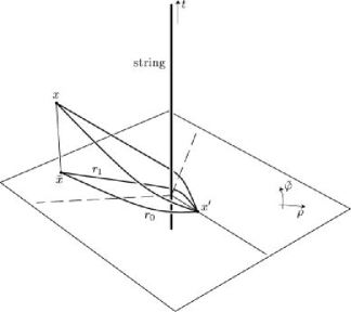
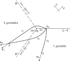
Figure 1: Three-dimensional spacetime diagram of the plane orthogonal to the cosmic string (i.e., the spacetime diagram with coordinate ${z}$ is suppressed). A rescaled coordinate ${{\tilde{\varphi}}=\nu\varphi}$ (periodic with the period ${2\pi}$) is used instead of ‘geometrical’ angular coordinate ${\varphi\in(-\pi/\nu,\pi/\nu)}$. Two spacetime points ${x}$ and ${x^{\prime}}$ can be joined by more than one geodesic as indicated in the diagram. The geodesics ‘bend’ around the string due to the curvature localized on the string. Of course, the ‘bending’ of the geodesics is only apparent—it arises because the rescaled coordinate ${{\tilde{\varphi}}}$ is employed. The geodesics are straight lines in locally flat geometry. However, the cosmic string causes the angle deficit and the intersection of geodesics behind the string is a real effect. Spatial projection of the geodesics into hypersurface ${t=\text{constant}}$ is also shown. These are spatial geodesics with length ${r_{k}}$. Also cf. Fig. 5.

where ${\eta}$ and ${r_{k}}$ are defined as

$\displaystyle\operatorname{ch}\eta=\frac{\Delta t^{2}-\Delta z^{2}-\rho^{2}-\rho^{\prime 2}}{2\rho\rho^{\prime}}{\mbox{\;,}}$ (15)
$\displaystyle r_{k}^{2}=\Delta z^{2}+\rho^{2}+\rho^{\prime 2}-2\rho\rho^{\prime}\cos\bigl{(}\Delta\varphi+2\pi k/\nu\bigr{)}{\mbox{\;,}}$ (16)

and ${\theta(t)}$ is the Heaviside step function. As we will discuss in detail below, index ${k\in{\mathbb{Z}}}$ labels spacetime geodesics joining points ${x}$ and ${x^{\prime}}$; its range ${{k_{{\mathrm{i}}}}(\Delta\varphi),\dots,{k_{{\mathrm{f}}}}(\Delta\varphi)}$ is given by conditions222For brevity, we will not write the dependence of ${{k_{{\mathrm{i}}}}}$ and ${{k_{{\mathrm{f}}}}}$ on angle ${\Delta\varphi}$ explicitly.

$$\begin{gathered}\Delta\varphi+2\pi({k_{{\mathrm{i}}}}-1)/\nu<-\pi<\Delta\varphi+2\pi{k_{{\mathrm{i}}}}/\nu{\mbox{\;,}}\\ \Delta\varphi+2\pi{k_{{\mathrm{f}}}}/\nu<\pi<\Delta\varphi+2\pi({k_{{\mathrm{f}}}}+1)/\nu{\mbox{\;.}}\end{gathered}$$ (17)
Refer to caption
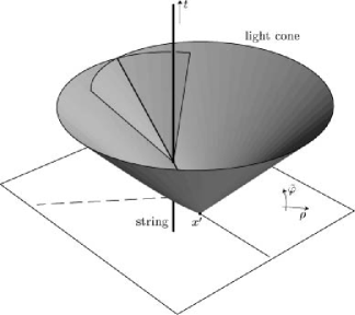
Figure 2: The support of the geodesic part ${{\boldsymbol{G}}^{\mspace{2.0mu}{\mathrm{gd}}}(x|x^{\prime})}$ of the Green function is localized on the future light cone of the source point ${x^{\prime}}$, i.e., on the null hypersurface generated by future null geodesics from ${x^{\prime}}$. Near vertex ${x^{\prime}}$ the hypersurface has the standard structure of the light cone in Minkowski spacetime. However, at the cosmic string the light cone deforms—it intersects itself and becomes a hypersurface with a boundary (given by null rays propagating near the string).

In (5) we separated the field equations into independent ones for components ${A_{t},A_{z},A_{\mu},A_{\bar{\mu}}}$. Now we can combine the Green functions ${{}^{\sigma}\!G^{{\mathrm{ret}}}(x|x^{\prime})}$ back to the full vector Green function:

$$\begin{split}{\boldsymbol{G}}^{\mspace{2.0mu}{\mathrm{ret}}}_{{\boldsymbol{ab}}^{\prime}}(x|x^{\prime})&=\bigl{(}-\,\mathbf{d}_{{\boldsymbol{a}}}t\,\mathbf{d}_{{\boldsymbol{b}}^{\prime}}t+\mathbf{d}_{{\boldsymbol{a}}}z\,\mathbf{d}_{{\boldsymbol{b}}^{\prime}}z\bigr{)}{}^{0}\!G^{{\mathrm{ret}}}(x|x^{\prime})\\ &\;\;+{{\boldsymbol{\mu}}}_{{\boldsymbol{a}}}\,{\bar{{\boldsymbol{\mu}}}}_{{\boldsymbol{b}}^{\prime}}{}^{+1}\!G^{{\mathrm{ret}}}(x|x^{\prime})+{\bar{{\boldsymbol{\mu}}}}_{{\boldsymbol{a}}}\,{{\boldsymbol{\mu}}}_{{\boldsymbol{b}}^{\prime}}{}^{-1}\!G^{{\mathrm{ret}}}(x|x^{\prime}){\mbox{\;,}}\end{split}$$ (18)

with unprimed and primed tensor indices considered at point ${x}$ and ${x^{\prime}}$, respectively. As a consequence of (5) and (12) the vector Green function satisfies the conditions analogous to (12) with the wave operator from Eq. (2).

This Green function can be split into two pieces with clear interpretation,

$${\boldsymbol{G}}^{\mspace{2.0mu}{\mathrm{ret}}}_{{\boldsymbol{ab}}^{\prime}}(x|x^{\prime})={\boldsymbol{G}}^{\mspace{2.0mu}{\mathrm{gd}}}_{{\boldsymbol{ab}}^{\prime}}(x|x^{\prime})+{\boldsymbol{G}}^{\mspace{2.0mu}{\mathrm{sc}}}_{{\boldsymbol{ab}}^{\prime}}(x|x^{\prime}){\mbox{\;.}}$$ (19)

The first geodesic part

$${\boldsymbol{G}}^{\mspace{2.0mu}{\mathrm{gd}}}_{{\boldsymbol{ab}}^{\prime}}(x|x^{\prime})=\frac{1}{2\pi}\,\theta(\Delta t)\sum_{k={k_{{\mathrm{i}}}}}^{{k_{{\mathrm{f}}}}}{{\boldsymbol{\iota}}}_{{\boldsymbol{ab}}^{\prime}}[\gamma_{k}]\,\delta\bigl{(}-\Delta t^{2}+r_{k}^{2}\bigr{)}$$ (20)

describes the propagation of the electromagnetic field along the null rays as in an empty flat spacetime. Here ${\gamma_{k}}$, ${k={k_{{\mathrm{i}}}},\dots,{k_{{\mathrm{f}}}}}$ are geodesics joining points ${x}$ and ${x^{\prime}}$, and ${{{\boldsymbol{\iota}}}_{{\boldsymbol{ab}}^{\prime}}[\gamma]}$ is the operator of parallel transport along the geodesic ${\gamma}$. Quantity ${r_{k}}$ defined in (16) is the spatial length of the ${k}$-th geodesic, see Fig. 1. Delta-functions in (20) enforce that the field propagates only along null geodesics. The only difference from the Minkowski spacetime is that light rays ‘bend’ around the cosmic string. If we call light cone of the source point ${x^{\prime}}$ a hypersurface generated by null geodesics from ${x^{\prime}}$ we see that it ‘deforms’ when it intersects the string – see Fig. 2. The contribution to the field with the source at point ${x^{\prime}}$ described by the geodesic part (20) is fully localized on this light cone.

Refer to caption
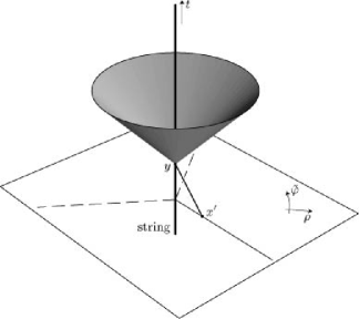
Figure 3: The support of the scattered part ${{\boldsymbol{G}}^{\mspace{2.0mu}{\mathrm{sc}}}(x|x^{\prime})}$ of the Green function is localized inside light cones with vertices ${y}$ on the cosmic string which are connected with the source by null geodesics. In the figure only a spacetime diagram of the plane going through the charge orthogonally to the string is shown. The electromagnetic field given by ${{\boldsymbol{G}}^{\mspace{2.0mu}{\mathrm{sc}}}(x|x^{\prime})}$ can be interpreted as the electromagnetic field scattered on the singular curvature localized on the string.

If we transform 1-forms ${{{\boldsymbol{\mu}}},{\bar{{\boldsymbol{\mu}}}}}$ back to the coordinate 1-forms ${\mathbf{d}\rho}$ and ${\mathbf{d}\varphi}$, the second part, ${{\boldsymbol{G}}^{\mspace{2.0mu}{\mathrm{sc}}}(x|x^{\prime})}$, of the Green function becomes

$$\begin{split}&{\boldsymbol{G}}^{\mspace{2.0mu}{\mathrm{sc}}}_{{\boldsymbol{ab}}^{\prime}}(x|x^{\prime})=-\frac{\nu}{8\pi^{2}}\frac{\theta(\Delta t)\,\theta\bigl{(}\Delta t^{2}\!-\!\Delta z^{2}\!-\!(\rho\!+\!\rho^{\prime})^{2}\bigr{)}}{\rho\rho^{\prime}}\\ &\quad\times\biggl{[}\biggl{(}\!\bigl{(}-\,\mathbf{d}_{{\boldsymbol{a}}}t\,\mathbf{d}_{{\boldsymbol{b}}^{\prime}}t+\mathbf{d}_{{\boldsymbol{a}}}z\,\mathbf{d}_{{\boldsymbol{b}}^{\prime}}z\bigr{)}\!\!-\!\bigl{(}\mathbf{d}_{{\boldsymbol{a}}}\rho\,\mathbf{d}_{{\boldsymbol{b}}^{\prime}}\rho+\rho\rho^{\prime}\mathbf{d}_{{\boldsymbol{a}}}\varphi\,\mathbf{d}_{{\boldsymbol{b}}^{\prime}}\varphi\bigr{)}\operatorname{ch}\eta\biggr{)}\frac{1}{\operatorname{sh}\eta}\biggl{(}\frac{\sin\nu(\pi-\Delta\varphi)}{\operatorname{ch}\nu\eta\!-\!\cos\nu(\pi\!-\!\Delta\varphi)}+\!\frac{\sin\nu(\pi+\Delta\varphi)}{\operatorname{ch}\nu\eta\!-\!\cos\nu(\pi\!+\!\Delta\varphi)}\biggr{)}\\ &\mspace{50.0mu}+\bigl{(}\rho\,\mathbf{d}_{{\boldsymbol{a}}}\varphi\,\mathbf{d}_{{\boldsymbol{b}}^{\prime}}\rho-\rho^{\prime}\,\mathbf{d}_{{\boldsymbol{a}}}\rho\,\mathbf{d}_{{\boldsymbol{b}}^{\prime}}\varphi\bigr{)}\,\biggl{(}\frac{\operatorname{sh}\nu\eta}{\operatorname{ch}\nu\eta\!-\!\cos\nu(\pi\!-\!\Delta\varphi)}-\frac{\operatorname{sh}\nu\eta}{\operatorname{ch}\nu\eta\!-\!\cos\nu(\pi\!+\!\Delta\varphi)}\biggr{)}\biggr{]}{\mbox{\;.}}\end{split}$$ (21)

It can be associated with a scattering on the ‘curvature’ localized on the string. Indeed, the contribution to the field due to this part of the Green function is localized in the causal future of points ${y}$ on the string which are connected to the source point ${x^{\prime}}$ by null geodesics – see Fig. 3. This fact is a simple manifestation of general behavior of the propagation of the electromagnetic field in a curved spacetime DeWitt and Brehme (1960): the main part propagates along null rays and is supported on the light cone of the source point. However, the field is scattered by curvature and propagates also inside light cone of the source point. This is the ‘tail-part’ of the field. It is easily seen that ${{\boldsymbol{G}}^{\mspace{2.0mu}{\mathrm{sc}}}(x|x^{\prime})}$ vanishes for ${\nu=1}$ (Minkowski space). The analogous behavior was also found in Refs. Khusnutdinov (1995); Aliev and Galtsov (1989) where the field of a general pointlike source was discussed.

III Electric field of the static charge and dipole

Refer to caption
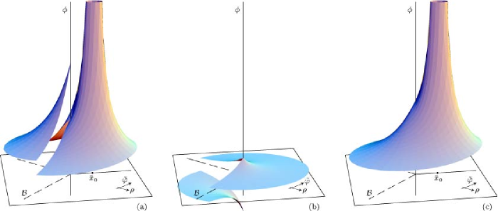
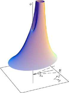
Figure 4: The graph of the scalar potential of a static charge near a cosmic string. Horizontal plane corresponds to the plane of the charge orthogonal to the cosmic string. The values of the scalar potential are drawn in the vertical direction. The full potential (22) (diagram (c)) is split into the geodesic part (a) and the scattered part (b). The whole potential is smooth except at the locations of the charge and at the string. Both geodesic and scattered parts are discontinuous at surfaces ${\mathcal{B}}$ where a number of spatial geodesics from the charge changes (cf. Fig. 5), however, the discontinuity of these two parts of the Green function cancels each other out. The scattered part of the field is finite and smooth near the charge; this part is responsible for self-interaction of the charge.

The Green function (18) can be used to derive the electric field of the static charge. Let us consider charge ${e}$ at ${z=z_{\mathrm{o}}}$, ${\rho=\rho_{\mathrm{o}}}$, and ${\varphi=\varphi_{\mathrm{o}}}$. The integration of the Green function over the electric current ${{\boldsymbol{J}}}$ simplifies: the source is static and only the time component of the vector potential survives; the integration over delta-functions of the geodesic part reduces to a simple sum; and thanks to the step functions in (21) the scattered part leads to the integration in proper time ${\tau}$ over half line only. Introducing the scalar potential ${\phi(x)=-A_{t}(x)}$ we get

$$\begin{split}&\phi(x)=\frac{e}{4\pi}\sum_{k={k_{{\mathrm{i}}}}}^{{k_{{\mathrm{f}}}}}\frac{1}{r_{k}}\\ &\quad-\frac{\nu e}{8\pi^{2}}\int_{0}^{\infty}\frac{S(\eta,\Delta\varphi)\,d\eta}{\sqrt{\Delta z^{2}+\rho^{2}+\rho_{\mathrm{o}}^{2}+2\rho\rho_{\mathrm{o}}\operatorname{ch}\eta}}{\mbox{\;.}}\end{split}$$ (22)

Here we defined function ${S}$ by

$$S(\eta,\varphi)=\frac{\sin\nu(\pi-\varphi)}{\operatorname{ch}\nu\eta\!-\!\cos\nu(\pi\!-\!\varphi)}+\frac{\sin\nu(\pi+\varphi)}{\operatorname{ch}\nu\eta\!-\!\cos\nu(\pi\!+\!\varphi)}{\mbox{\;,}}$$ (23)

and we used notation

$\displaystyle\Delta z=z-z_{\mathrm{o}}{\mbox{\;,\quad}}\Delta\varphi=\varphi-\varphi_{\mathrm{o}}{\mbox{\;,}}$ (24)
$\displaystyle r_{k}^{2}=\Delta z^{2}+\rho^{2}+\rho_{\mathrm{o}}^{2}-2\rho\rho_{\mathrm{o}}\cos\bigl{(}\Delta\varphi+2\pi k/\nu\bigr{)}{\mbox{\;.}}$

The first term—the sum in (22)—has the origin in the geodesic part of the Green function, the integral term arises from the scattered part. In derivation of this term we changed the integration over proper time ${\tau}$ into the integration over ${\eta}$ using the substitution

$$\operatorname{ch}\eta=\frac{(t-\tau)^{2}-\Delta z^{2}-\rho^{2}-\rho_{\mathrm{o}}^{2}}{2\rho\rho_{\mathrm{o}}}{\mbox{\;.}}$$ (25)

For a graphical representation of the scalar potential, see Fig. 4.

The electric field ${{\boldsymbol{E}}=E^{\hat{\rho}}{\boldsymbol{e}}_{\rho}+E^{\hat{\varphi}}{\boldsymbol{e}}_{\varphi}+E^{\hat{z}}{\boldsymbol{e}}_{z}}$ implied by (22), evaluated with respect to the normalized triad ${\{{\boldsymbol{e}}_{\rho},\,{\boldsymbol{e}}_{\varphi},\,{\boldsymbol{e}}_{z}\}}$ (i.e., ${{\boldsymbol{e}}_{\rho}={{\boldsymbol{\partial}}_{\rho}}}$, ${{\boldsymbol{e}}_{\varphi}=\rho^{-1}{{\boldsymbol{\partial}}_{\varphi}}}$, ${{\boldsymbol{e}}_{z}={{\boldsymbol{\partial}}_{z}}}$) is

$$\begin{split}E^{\hat{z}}&=\frac{e}{4\pi}\sum_{k={k_{{\mathrm{i}}}}}^{{k_{{\mathrm{f}}}}}\frac{\Delta z}{r_{k}^{3}}\\ &\quad-\frac{\nu e}{8\pi^{2}}\int_{0}^{\infty}\frac{S(\eta,\Delta\varphi)\,\Delta z\,d\eta}{\bigl{(}\Delta z^{2}+\rho^{2}+\rho_{\mathrm{o}}^{2}+2\rho\rho_{\mathrm{o}}\operatorname{ch}\eta\bigr{)}^{3/2}}{\mbox{\;,}}\end{split}$$
$$\begin{split}E^{\hat{\rho}}&=\frac{e}{4\pi}\sum_{k={k_{{\mathrm{i}}}}}^{{k_{{\mathrm{f}}}}}\frac{\rho-\rho_{\mathrm{o}}\cos(\Delta\varphi+2\pi k/\nu)}{r_{k}^{3}}\\ &\quad-\frac{\nu e}{8\pi^{2}}\int_{0}^{\infty}\frac{S(\eta,\Delta\varphi)\,(\rho+\rho_{\mathrm{o}}\operatorname{ch}\eta)\,d\eta}{\bigl{(}\Delta z^{2}+\rho^{2}+\rho_{\mathrm{o}}^{2}+2\rho\rho_{\mathrm{o}}\operatorname{ch}\eta\bigr{)}^{3/2}}{\mbox{\;,}}\end{split}$$ (26)
$$\begin{split}E^{\hat{\varphi}}&=\frac{e}{4\pi}\sum_{k={k_{{\mathrm{i}}}}}^{{k_{{\mathrm{f}}}}}\frac{\rho_{\mathrm{o}}\sin(\Delta\varphi+2\pi k/\nu)}{r_{k}^{3}}\\ &\quad+\frac{\nu e}{8\pi^{2}}\int_{0}^{\infty}\frac{\frac{\partial S}{\partial\varphi}(\eta,\Delta\varphi)\,d\eta}{\rho\bigl{(}\Delta z^{2}+\rho^{2}+\rho_{\mathrm{o}}^{2}+2\rho\rho_{\mathrm{o}}\operatorname{ch}\eta\bigr{)}^{1/2}}{\mbox{\;.}}\end{split}$$

Geodesic part has a clear meaning—it is a sum of the ‘Coulomb’ terms corresponding to different spatial geodesics joining the charge and the field point. Indeed, it has the form

$${\boldsymbol{E}}^{{\mathrm{gd}}}(x)=\sum_{k={k_{{\mathrm{i}}}}}^{{k_{{\mathrm{f}}}}}\frac{e}{4\pi}\,\frac{1}{r_{k}^{2}}\,{\boldsymbol{e}}_{k}{\mbox{\;,}}$$ (27)

where, ${{\boldsymbol{e}}_{k}}$ is a unit vector tangent to the ${k}$-th spatial geodesic joining ${\bar{x}_{\mathrm{o}}}$ and ${\bar{x}}$—the spatial projections (projections to the hypersurface ${t=\text{constant}}$) of the charge and of the field point ${x}$, cf. Fig. 5. Clearly, the geodesic part of the field is discontinuous on surfaces on one side of which points are connected to the charge by different number of geodesics than on other side. However, the whole electric field (26) is continuous here. The discontinuity is compensated by the scattered part of the field; cf. the graphs for the scalar potential in Fig. 4.

Refer to caption
Figure 5: The spatial diagram of the hypersurface ${t=\text{constant}}$ (cf. spacetime diagram in Fig. 1). Points ${\bar{x}}$ and ${\bar{x}_{\mathrm{o}}}$ are spatial projections of spacetime point ${x}$ and of the worldline of the static charge. Rescaled coordinate ${\tilde{\varphi}=\nu\varphi}$ is used. geodesic part (27) of the electric field at ${\bar{x}}$ of the charge at ${\bar{x}_{\mathrm{o}}}$ is given by standard flat-space Coulomb contributions for each spatial geodesic joining ${\bar{x}}$ and ${\bar{x}_{\mathrm{o}}}$. Surface ${\mathcal{B}}$ (indicated by dashed line) divides the space into domains, points of which are connected with the charge by one geodesic or by two geodesics, respectively. For sufficiently large angle deficit there exist also points connected with the charge by more geodesics.

Near the cosmic string we can observe an interesting phenomenon: the charge is self-interacting with itself. Of course, the field evaluated at the charge is infinite. However, if we subtract the standard Coulomb field near the charge, we obtain a finite residual field which acts on the charge itself. The regularized potential energy of the charge in its field is equal to

$$W^{\mathrm{self}}(\bar{x}_{\mathrm{o}})=\frac{e}{2}\Bigl{(}\phi-\frac{e}{4\pi}\frac{1}{r_{0}}\Bigr{)}\Big{|}_{x_{\mathrm{o}}}=C\frac{e^{2}}{\rho_{\mathrm{o}}}{\mbox{\;,}}$$ (28)

with the constant ${C}$ given by333${\lfloor\nu/2\rfloor}$ denotes an integer part of ${\nu/2}$. Indeed, conditions (17) for ${\Delta\varphi=0}$ give ${{k_{{\mathrm{f}}}}=-{k_{{\mathrm{i}}}}=\lfloor\nu/2\rfloor}$, and ${k=0}$ term is removed by the regularization. For ${\nu<2}$ the sum contains thus no terms.

$$C=\frac{1}{8\pi}\sum_{k=1}^{\lfloor\nu/2\rfloor}\frac{1}{\sin\frac{\pi k}{\nu}}-\frac{\nu\,\sin\nu\pi}{16\,\pi^{2}}\int_{0}^{\infty}\!\!\!\!\frac{\operatorname{ch}^{\!-\!1}\!\frac{\eta}{2}}{\operatorname{ch}\nu\eta-\cos\nu\pi}\,d\eta{\mbox{\;.}}$$ (29)

The self-force is

$${\boldsymbol{F}}^{\,{\mathrm{self}}}=C\frac{e^{2}}{\rho_{\mathrm{o}}^{2}}\;{\boldsymbol{e}}_{\rho}{\mbox{\;.}}$$ (30)

The result (22) and the prediction of the self-interaction are not new. They are equivalent to the result of Ref. Linet (1986) which was obtained by a direct solution of the three-dimensional Laplace equation in the space with angle deficit. Nevertheless, our form is more useful for the calculation of self-force (30) since we can easily subtract the divergent flat space contribution which correspond to the ${k=0}$ term in sums in (22) and (26). The self-interaction of a general source was also discussed in Refs. Khusnutdinov (1995); Aliev and Galtsov (1989).

Using the electric field of the static point charge it is straightforward to find the field of an electric dipole at ${\bar{x}_{\mathrm{o}}}$ with the spatial charge distribution given by ${-{\boldsymbol{p}}^{{\boldsymbol{n}}}\mathbf{\nabla}_{{\boldsymbol{n}}}\delta(\bar{x}|\bar{x}_{\mathrm{o}})}$. For ${{\boldsymbol{p}}=p^{\hat{z}}{\boldsymbol{e}}_{z}+p^{\hat{\rho}}{\boldsymbol{e}}_{\rho}+p^{\hat{\varphi}}{\boldsymbol{e}}_{\varphi}}$ the potential is

$$\begin{split}\phi=&\,\frac{1}{4\pi}\sum_{k={k_{{\mathrm{i}}}}}^{k_{{\mathrm{f}}}}\frac{1}{r_{k}^{3}}\Bigr{[}\Delta z\,p^{\hat{z}}-\bigl{(}\rho_{\mathrm{o}}-\rho\cos\Delta\varphi_{k}\bigr{)}p^{\hat{\rho}}\\[-12.91663pt] &\mspace{240.0mu}+\rho\sin\Delta\varphi_{k}\,p^{\hat{\varphi}}\Bigr{]}\\[4.30554pt] &+\frac{\nu}{8\pi^{2}}\int_{0}^{\infty}\biggl{[}\frac{S(\eta,\Delta\varphi)\bigl{(}-\Delta z\,p^{\hat{z}}+(\rho_{\mathrm{o}}\!+\!\rho\operatorname{ch}\eta)p^{\hat{\rho}}\bigr{)}}{\bigl{(}\Delta z^{2}+\rho^{2}+\rho_{\mathrm{o}}^{2}+2\rho\rho_{\mathrm{o}}\operatorname{ch}\eta\bigr{)}^{3/2}}\\ &\mspace{100.0mu}+\frac{\rho_{\mathrm{o}}^{-1}\;\frac{\partial S}{\partial\varphi}(\eta,\Delta\varphi)\,p^{\hat{\varphi}}}{\bigl{(}\Delta z^{2}+\rho^{2}+\rho_{\mathrm{o}}^{2}+2\rho\rho_{\mathrm{o}}\operatorname{ch}\eta\bigr{)}^{1/2}}\biggr{]}\,d\eta{\mbox{\;,}}\end{split}$$ (31)

where ${\Delta\varphi_{k}=\Delta\varphi+2\pi k/\nu}$.

The action of the dipole on itself can be obtained from the (regularized) self-energy of the dipole in its own field defined analogously to (28). Calculations lead to

$$W^{\mathrm{self}}(\bar{x}_{\mathrm{o}},{\boldsymbol{p}})=\frac{1}{\rho_{\mathrm{o}}^{3}}\,\Bigl{(}C_{(z)}(p^{\hat{z}})^{2}+C_{(\rho)}(p^{\hat{\rho}})^{2}-C_{(\varphi)}(p^{\hat{\varphi}})^{2}\Bigr{)}{\mbox{\;,}}$$ (32)

where positive444For ${\nu<2}$, the positivity of ${C_{(\rho)}}$ and ${C_{(z)}}$ follows immediately from expressions (33). The positivity for ${\nu>2}$ and the positivity of ${C_{(\varphi)}}$ was checked numerically. constants ${C_{(\rho)}}$, ${C_{(z)}}$, and ${C_{(\varphi)}}$ are given by

$\displaystyle C_{(z)}\!$ $\displaystyle=\frac{1}{16\pi}\!\!\sum_{k=1}^{\lfloor\nu/2\rfloor}\!\frac{1}{\sin^{3}\frac{\pi k}{\nu}}-\frac{\nu\,\sin\nu\pi}{32\,\pi^{2}}\!\!\int_{0}^{\infty}\!\!\!\!\frac{\operatorname{ch}^{\!-\!3}\!\frac{\eta}{2}}{\operatorname{ch}\nu\eta\!-\!\cos\nu\pi}\,d\eta{\mbox{\;,}}\allowdisplaybreaks$
$\displaystyle\begin{split}C_{(\rho)}\!&=\frac{1}{32\pi}\!\sum_{k=1}^{\lfloor\nu/2\rfloor}\frac{3-\cos\frac{2\pi k}{\nu}}{\sin^{3}\frac{\pi k}{\nu}}\\ &\;\quad-\frac{\nu\,\sin\nu\pi}{64\,\pi^{2}}\int_{0}^{\infty}\!\!\!\frac{1}{\operatorname{ch}^{3}\!\frac{\eta}{2}}\,\frac{3+\operatorname{ch}\eta}{\operatorname{ch}\nu\eta\!-\!\cos\nu\pi}\,d\eta{\mbox{\;,}}\end{split}\allowdisplaybreaks$ (33)
$\displaystyle\begin{split}C_{(\varphi)}\!&=\frac{1}{32\pi}\!\sum_{k=1}^{\lfloor\nu/2\rfloor}\frac{3+\cos\frac{2\pi k}{\nu}}{\sin^{3}\frac{\pi k}{\nu}}\\ &\;\quad+\frac{\nu^{3}\,\sin\nu\pi}{8\,\pi^{2}}\int_{0}^{\infty}\!\!\!\frac{1}{\operatorname{ch}\!\frac{\eta}{2}}\,\frac{\operatorname{ch}^{2}\!\nu\eta\!+\!\operatorname{ch}\nu\eta\cos\nu\pi\!-\!2}{(\operatorname{ch}\nu\eta\!-\!\cos\nu\pi)^{3}}\,d\eta{\mbox{\;.}}\end{split}$

The dipole is acting on itself by force

$${\boldsymbol{F}}^{\,{\mathrm{self}}}=-\bar{\mathbf{\nabla}}W^{\mathrm{self}}(\bar{x}_{\mathrm{o}},{\boldsymbol{p}})$$ (34)

and by a torque

$${\boldsymbol{\tau}}^{\,{\mathrm{self}}}=-{\boldsymbol{p}}\times\frac{\partial W^{\mathrm{self}}}{\partial{\boldsymbol{p}}}(\bar{x}_{\mathrm{o}},{\boldsymbol{p}}){\mbox{\;,}}$$ (35)

where ${\bar{\mathbf{\nabla}}}$ is spatial covariant derivative and ${\times}$ spatial cross-product.

Observing the structure of the self-energy (32) we see that the torque is vanishing if the dipole is parallel to directions ${{\boldsymbol{e}}_{\rho}}$, ${{\boldsymbol{e}}_{z}}$, or ${{\boldsymbol{e}}_{\varphi}}$; the equilibrium is stable for direction ${{\boldsymbol{e}}_{\varphi}}$. The self-force is repulsive from the string for the dipole along ${{\boldsymbol{e}}_{\rho}}$ and ${{\boldsymbol{e}}_{z}}$ directions, and it is attractive towards the string for the dipole along ${{\boldsymbol{e}}_{\varphi}}$ direction.

IV Magnetic field of the current parallel to the string

Analogous results can be obtained also in the case of only two relevant spatial dimensions, i.e., with the sources distributed homogeneously along the string. The simplest interesting example is the field of the static electric current ${I}$ flowing in the ${z}$ direction along the line at a distance ${\rho_{\mathrm{o}}}$ from the string. It follows from the Green function (18) that for the current in the ${z}$ direction the only nonvanishing component of the vector potential is ${A_{z}}$, and it is given by the same scalar Green function as in the electrostatic case. Integrating the Green function over the world-sheet of the line splits into the integration over the time direction—which is equivalent to the integration performed in the previous section—and to the integration over the ${z}$ direction. The latter integration diverges because of an infinite length of the source, however, this divergence can be removed shifting the potential by an infinite constant555This divergence is not related to the string—the same situation occurs also in empty Minkowski spacetime.. For the ${z}$ component of the vector potential we obtain

$$\begin{split}&A_{z}(x)=-\frac{I}{2\pi}\sum_{k={k_{{\mathrm{i}}}}}^{{k_{{\mathrm{f}}}}}\ln{s_{k}}\\ &\quad+\frac{\nu I}{8\pi^{2}}\int_{0}^{\infty}S(\eta,\Delta\varphi)\ln\bigl{(}{\rho^{2}+\rho_{\mathrm{o}}^{2}+2\rho\rho_{\mathrm{o}}\operatorname{ch}\eta}\bigr{)}\,d\eta{\mbox{\;,}}\end{split}$$ (36)

with ${S(\eta,\varphi)}$ defined again by (23) and

$$s_{k}=\sqrt{\rho^{2}+\rho_{\mathrm{o}}^{2}-2\rho\rho_{\mathrm{o}}\cos\bigl{(}\Delta\varphi+2\pi k/\nu\bigr{)}}$$ (37)

being the distance from the line along the ${k}$-th geodesic orthogonal to the line. Magnetic field ${{\boldsymbol{B}}=B^{\hat{z}}{\boldsymbol{e}}_{z}+B^{\hat{\rho}}{\boldsymbol{e}}_{\rho}+B^{\hat{\varphi}}{\boldsymbol{e}}_{\varphi}}$ is then given by

$\displaystyle\begin{split}B^{\hat{\rho}}&=-\frac{I}{2\pi}\sum_{k={k_{{\mathrm{i}}}}}^{{k_{{\mathrm{f}}}}}\frac{\rho_{\mathrm{o}}\sin(\Delta\varphi+2\pi k/\nu)}{s_{k}^{2}}\\ &\mspace{-30.0mu}+\frac{\nu I}{8\pi^{2}}\int_{0}^{\infty}\frac{1}{\rho}\,\frac{\partial S}{\partial\varphi}(\eta,\Delta\varphi)\,\ln\bigl{(}\rho^{2}+\rho_{\mathrm{o}}^{2}+2\rho\rho_{\mathrm{o}}\operatorname{ch}\eta\bigr{)}\,d\eta{\mbox{\;,}}\end{split}$
$\displaystyle B^{\hat{z}}$ $\displaystyle=0{\mbox{\;,}}$ (38)
$\displaystyle\begin{split}B^{\hat{\varphi}}&=\frac{I}{2\pi}\sum_{k={k_{{\mathrm{i}}}}}^{{k_{{\mathrm{f}}}}}\frac{\rho-\rho_{\mathrm{o}}\cos(\Delta\varphi+2\pi k/\nu)}{s_{k}^{2}}\\ &\quad-\frac{\nu I}{4\pi^{2}}\int_{0}^{\infty}\frac{S(\eta,\Delta\varphi)\,(\rho+\rho_{\mathrm{o}}\operatorname{ch}\eta)\,d\eta}{\rho^{2}+\rho_{\mathrm{o}}^{2}+2\rho\rho_{\mathrm{o}}\operatorname{ch}\eta}{\mbox{\;.}}\end{split}$

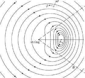
The magnetic lines for such a field are shown in Fig. 6. We observe that they have the standard structure of the magnetic field around a straight line current except that they are deformed near the string. We will discuss this deformation more in the following section.

Refer to caption
Figure 6: Magnetic lines around the electric current along the line through ${\bar{x}_{\mathrm{o}}}$ parallel to the string. Planes ${\mathcal{B}}$ (indicated by dashed lines) separate the space into domains in which the points are connected with the source by one, respectively two geodesics. A rather large value ${\nu=1.8}$ of the inverse conicity parameter was chosen to emphasize the deformation of magnetic lines near the string. As discussed in Sec. VI, for physically relevant values, ${\nu\approx 1}$, the domain near the string in which the magnetic lines are deformed is too small to be visualized (cf. also Fig. 8).

Similarly to the self-force (30) of the static charge the current line acts on itself by a self-force which is now, however, pushing the source towards the string. Subtracting the standard empty space contribution to the magnetic field at the position of the line the force on the line leads to

$${\boldsymbol{F}}^{\,{\mathrm{self}}}=-\frac{I^{2}}{4\pi\rho_{\mathrm{o}}}\,(\nu-1)\;{\boldsymbol{e}}_{\rho}$$ (39)

(here we used integral (60) from the appendix).

V The field at large distances from the string

Expanding the potential (22) of a static charge at a large distance ${r\gg\rho_{\mathrm{o}}}$ from the origin (located on the string, i.e., assuming ${\Delta z=r\cos\vartheta}$, ${\rho=r\sin\vartheta}$), we obtain

$$\begin{split}\phi=&\frac{e}{4\pi}\frac{1}{r}\sum_{k={k_{{\mathrm{i}}}}}^{k_{{\mathrm{f}}}}\Bigl{[}1+\frac{\rho_{\mathrm{o}}}{r}\sin\vartheta\cos\Delta\varphi_{k}+{\mathcal{O}}\Bigl{(}\frac{\rho_{\mathrm{o}}^{2}}{r^{2}}\Bigr{)}\Bigr{]}\\ &-\frac{\nu e}{8\pi^{2}}\frac{1}{r}\int_{0}^{\infty}\!\!\!\!S(\eta,\Delta\varphi)\Bigl{[}1-\frac{\rho_{\mathrm{o}}}{r}\sin\vartheta\operatorname{ch}\eta+{\mathcal{O}}\Bigl{(}\frac{\rho_{\mathrm{o}}^{2}}{r^{2}}\Bigl{)}\Bigr{]}d\eta{\mbox{\;.}}\end{split}$$ (40)

Using integrals (60) and (62) from Appendix B we get

$$\phi=\frac{1}{4\pi}\frac{\nu e}{r}+\frac{1}{r}\,{\mathcal{O}}\Bigl{(}\frac{\rho_{\mathrm{o}}^{2}}{r^{2}}\Bigr{)}{\mbox{\;.}}$$ (41)

We see that the monopole contribution corresponds to the modified charge ${\nu e}$. The same result for the electric field ${{\boldsymbol{E}}}$ can be obtained using the Gauss law: the density of the electric flux (the magnitude of ${{\boldsymbol{E}}}$) at infinity has to be bigger to compensate the smaller area of a distant ‘sphere’ which, due to the conicity of space, grows only as ${4\pi r^{2}/\nu}$.

An interesting feature of the far field is the absence of a dipole term—indeed, the term proportional to ${r^{-2}}$ is missing in (41). This behavior can be confirmed investigating the far field of the dipole located near the string. The expansion of the potential (31) for large ${r}$ leads to

$$\begin{split}\phi=&\frac{1}{4\pi}\frac{1}{r^{2}}\sum_{k={k_{{\mathrm{i}}}}}^{{k_{{\mathrm{f}}}}}\Bigl{[}\cos\vartheta\,p^{\hat{z}}+\sin\vartheta\cos\Delta\varphi_{k}\,p^{\hat{\rho}}\\[-12.91663pt] &\mspace{240.0mu}+\sin\vartheta\sin\Delta\varphi_{k}\,p^{\hat{\varphi}}\Bigr{]}\\ &+\frac{\nu}{8\pi^{2}}\frac{1}{r}\int_{0}^{\infty}\frac{1}{\rho_{\mathrm{o}}}\frac{\partial S}{\partial\varphi}(\eta,\Delta\varphi)\,p^{\hat{\varphi}}\,d\eta\\ &+\frac{\nu}{8\pi^{2}}\frac{1}{r^{2}}\int_{0}^{\infty}\Bigl{[}\bigl{(}-\cos\vartheta\,p^{\hat{z}}+\sin\vartheta\operatorname{ch}\eta\,p^{\hat{\rho}}\bigr{)}S(\eta,\Delta\varphi)\\ &\mspace{165.0mu}-\sin\vartheta\operatorname{ch}\eta\,\frac{\partial S}{\partial\varphi}(\eta,\Delta\varphi)\,p^{\hat{\varphi}}\Bigr{]}d\eta\\[-4.30554pt] &+\frac{1}{r^{2}}{\mathcal{O}}\Bigl{(}\frac{\rho_{\mathrm{o}}}{r}\Bigr{)}{\mbox{\;.}}\end{split}$$ (42)

Substituting for the integrals expressions (60), (62), (66), and (69) we obtain

$$\phi=\frac{1}{4\pi}\frac{\nu\,p^{\hat{z}}\cos\vartheta}{r^{2}}+\frac{1}{r^{2}}{\mathcal{O}}\Bigl{(}\frac{\rho_{\mathrm{o}}}{r}\Bigr{)}{\mbox{\;.}}$$ (43)

We see that only the component ${p^{\hat{z}}}$ of the dipole parallel to the string contributes in the order ${r^{-2}}$. The field of the dipole oriented orthogonally to the string is suppressed at large distances; it falls-off as ${r^{-3}}$.

It is surprising that the suppression of ${r^{-2}}$ term for the dipole orthogonal to the string is non-smooth in the limit ${\nu\to 1}$, i.e., in the limit of the Minkowski spacetime: the ${r^{-2}}$ term is present for ${\nu=1}$, however, it vanishes for any ${\nu>1}$. It turns out that the Minkowski limit is achieved by an ‘enlarging’ the field’s near-by zone to infinity. In other words, a far zone, where the field is described by (41) or (43), starts at larger and larger distances with ${\nu}$ approaching ${1}$; and it disappears completely for ${\nu=1}$.

It is not very clear how to estimate a ‘size’ of the far zone analytically; however, a numerical analysis indicates that it ‘shrinks’ to infinity faster than any power of a deficit angle parameter ${1/(\nu-1)}$. One way how to determine the size of the far zone is to transform it to a domain near the string, using a spherical inversion with a center on the string. Such a domain near the string will be studied in the next section—cf., e.g., Fig. 8 for an estimate of its size.

In the Minkowski spacetime the conformal transformation of the electromagnetic field associated with the spherical inversion transforms the dipole field into a homogeneous field. The vanishing dipole term far from the string thus suggests a suppression of the homogeneous component of the field near the string. Let us study this property in more detail.

VI Suppression of the field of distant sources near the string

Expanding the scalar potential (22) of the static charge in the domain near the string, i.e., for ${\rho\ll\rho_{\mathrm{o}}}$, and using integrals (66), (62) we obtain

$$\begin{split}\phi&=\frac{e}{4\pi}\frac{1}{\rho_{\mathrm{o}}}\,\sum_{k={k_{{\mathrm{i}}}}}^{{k_{{\mathrm{f}}}}}\Bigl{(}1+\frac{\rho}{\rho_{\mathrm{o}}}\cos\Delta\varphi_{k}+{\mathcal{O}}\Bigl{(}{\frac{\rho^{2}}{\rho_{\mathrm{o}}^{2}}}\Bigr{)}\Bigr{)}\\ &\quad-\frac{\nu e}{8\pi^{2}}\frac{1}{\rho_{\mathrm{o}}}\int_{0}^{\infty}\!\!\Bigl{(}1-\frac{\rho}{\rho_{\mathrm{o}}}\,\operatorname{ch}\eta+{\mathcal{O}}\Bigl{(}{\frac{\rho^{2}}{\rho_{\mathrm{o}}^{2}}}\Bigr{)}\Bigr{)}\,S(\eta,\Delta\varphi)\,d\eta\\ &=\frac{e}{4\pi}\frac{1}{\rho_{\mathrm{o}}}+\frac{1}{\rho_{\mathrm{o}}}\,{\mathcal{O}}\Bigl{(}{\frac{\rho^{2}}{\rho_{\mathrm{o}}^{2}}}\Bigr{)}{\mbox{\;.}}\end{split}$$ (44)

Up to the linear order there is no term depending on a position—the scalar potential ${\phi}$ is constant near the string and hence, the electric field ${{\boldsymbol{E}}}$ is vanishing. This is a surprising result: it means that the field of large distant charges is suppressed near the cosmic string. In other words, it is possible to hide oneself near the string from the electric field of strong charges.

Refer to caption
Figure 7: Scalar potential of the static charge near the string with a ‘large’ deficit angle (namely, ${\nu=1.8}$). We can se that it has a small plateau near the string. The electric field ${{\boldsymbol{E}}}$ is suppressed here. Such a plateau exists for any value ${\nu\neq 1}$, however, it is very small for ${\nu}$ close to ${1}$, cf. Figs. 4 and 8.

The expulsion of the field away from the string is not continuous in the limit ${\nu\to 1}$: the electric field ${{\boldsymbol{E}}}$ is negligible near the string for any value ${\nu>1}$, but it is present for ${\nu=1}$. The limit of no string is actually realized by a contraction of a domain around the string in which the field is suppressed. For ${\nu}$ close to ${1}$ the domain of vanishing electric field is rather small. It is nontrivial only for ${\nu\gtrsim 3/2}$ (see Fig. 7), however it shrinks rapidly with ${\nu\to 1}$, as it is seen in Fig. 8. A numerical study indicates that a typical size of this domain decreases faster than any power of a deficit angle parameter ${\nu-1}$.

A similar discussion applies also for a magnetic field—e.g., the magnetic field discussed in Sec. IV is also suppressed near the string.

Refer to caption
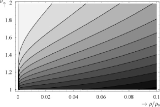
Figure 8: The diagram illustrates the dependence of a typical size of the domain near the string, where the electric field ${{\boldsymbol{E}}}$ of the static charge is suppressed, on the parameter ${\nu}$. To estimate a size of the domain, a value of the field is evaluated along a line going through the charge orthogonally to the string. The horizontal direction in the figure corresponds to the distance from the string. The vertical direction corresponds to different values of the parameter ${\nu}$. The contours of constant values of the field are drawn, with shading indicating the strength of the field (the shading is drawn only in discrete steps given by contours). For ${\nu>1.5}$, the interval of small field (light shading) is large; for ${\nu\to 1}$ this intervals shrinks very rapidly and it disappears for ${\nu=1}$. See also graphs of scalar potential for ${\nu=1.2}$ in Fig. 4(c) and for ${\nu=1.8}$ in Fig. 7. Only in the latter one a flat domain near the string can be easily identified. A similar analysis applies also for magnetic field ${{\boldsymbol{B}}}$ discussed in Sec. IV. A domain of the expulsion of magnetic lines near the string can be identified, e.g., in Fig. 6.

The behavior of the field can be also rephrased as a nonexistence of a homogeneous electric or magnetic field perpendicular to the cosmic string. Indeed, in empty Minkowski spacetime the homogeneous electric field can be constructed as a field of a large charge at large distances. As we have seen, in the spacetime of cosmic string the field of the charge located at large distances from the string is suppressed and there is thus no analogue of the homogeneous field perpendicular to the string. The same result can be obtained also by studying a general static field around the string (i.e., by a direct solution of the homogeneous Laplace equation in the space with a deficit angle) Krtouš (1989).

VII Summary

We have discussed the electromagnetic field in the spacetime of a cosmic string. The retarded Green function (14) for the vector potential was found. It can be split into a ‘geodetical’ part (20) corresponding to the empty space propagation of the field, and into a ‘scattered’ part (21) corresponding to scattering on the curvature located within the string.

Using this Green function electric and magnetic fields of various simple static sources were constructed. It was demonstrated that although the spacetime is locally flat (outside the string), the global deficit angle causes several interesting phenomena. We found a self-interaction of the point charge (repulsive away from the string), of the dipole (turning the dipole into the ${{\boldsymbol{e}}_{\varphi}}$ direction ‘around’ the string), or of the line current (attractive toward the string). In general, the self-interaction of charges and currents near the string implies that the string participates on electromagnetic processes even if it is not charged itself. It can have consequences when studying the motion of cosmic strings through, e.g., ionised plasma in an early Universe.

Further, we found that the field of a static source at large distances has a different multipole structure, namely, there is no dipole term corresponding to the dipole perpendicular to the string.

Near the string, the electric and magnetic fields orthogonal to the string are suppressed. For the same reason, there exists no homogeneous static field perpendicular to the string.

Most of the discussed effects can easily be understood in the special case ${\nu=2}$ (respectively, for ${\nu}$ being any integer). In this case the scattered part of the field vanishes and the resulting field can be obtained as the field in the half of Minkowski spacetime given by the real source and by a fictitious source obtained as a reflection of the real source with respect to the axis (these two contributions correspond to different terms in the sum over geodetics in (22)). The self-interaction is thus given by the interaction of the real and the fictitious sources. A suppression of the dipole field at large distances arises because a combination of the dipole (orthogonal to the string) and of its reflected image gives a quadrupole configuration. And finally, the expulsion of the field away from the string arises as a cancelation of the fields of the source and of its image in middle between them.

After deriving the general form of the Green function we concentrated mainly on static phenomena. As a next step it would be interesting to study similar questions in dynamical contexts; for example, the scattering of plane waves on the string or the field of a strong oscillating dipole located far from the string.

Acknowledgements.
The author would like to thank Prof. Gal’tsov for a guidance during author’s study stay at Lomonosov University in Moscow back in 1988, during which most of the work Krtouš (1989) was done, and Prof. Bičák for arranging this stay and for reading both Krtouš (1989) and the manuscript of this paper.

Appendix A Integration of the Green function

In this Appendix we evaluate the integral (13). The choice of the integration contour in the complex plane of ${\omega}$ guarantees that the integral is vanishing for ${\Delta t<0}$. For ${\Delta t>0}$ we can close the contour in the upper half of the complex plane and the integration over ${\omega}$ leads to residues at simple poles ${\omega=\pm\sqrt{\kappa^{2}+\lambda^{2}}}$. This gives

$$\begin{split}&{}^{\sigma}\!G^{{\mathrm{ret}}}(x|x^{\prime})=-\frac{i\nu}{(2\pi)^{2}}\;\theta(\Delta t)\sum_{n\in{\mathbb{Z}}}e^{-in\nu\Delta\varphi}\\ &\quad\times\int_{0}^{\infty}\!\!\lambda d\lambda\;\operatorname{J}_{\left\lvert\nu n+\sigma\right\rvert}(\lambda\rho)\,\operatorname{J}_{\left\lvert\nu n+\sigma\right\rvert}(\lambda\rho^{\prime})\int_{-\infty}^{\infty}\frac{d\kappa}{\sqrt{\lambda^{2}+\kappa^{2}}}\\ &\qquad\quad\times\frac{1}{2}\Bigl{(}e^{i\lambda\bigl{(}\sqrt{1+\frac{\kappa^{2}}{\lambda^{2}}}\Delta t-\frac{\kappa}{\lambda}\Delta z\bigr{)}}-e^{-i\lambda\bigl{(}\sqrt{1+\frac{\kappa^{2}}{\lambda^{2}}}\Delta t+\frac{\kappa}{\lambda}\Delta z\bigr{)}}\Bigr{)}{\mbox{\;.}}\end{split}$$ (45)

Next we substitute for ${\kappa}$

$$\operatorname{sh}\alpha=\frac{\kappa}{\lambda}{\mbox{\;,\quad}}\operatorname{ch}\alpha=\sqrt{1+\frac{\kappa^{2}}{\lambda^{2}}}{\mbox{\;.}}$$ (46)

For ${\Delta z^{2}>\Delta t^{2}}$ we introduce the notation

$$\Delta t=s\operatorname{sh}\beta{\mbox{\;,\quad}}\Delta z=s\operatorname{ch}\beta{\mbox{\;,\quad}}\operatorname{sgn}s=\operatorname{sgn}\Delta z{\mbox{\;,}}$$ (47)

and we obtain

$$\begin{split}&{}^{\sigma}\!G^{{\mathrm{ret}}}(x|x^{\prime})=\frac{\nu}{(2\pi)^{2}}\;\theta(\Delta t)\,\theta\bigl{(}\Delta z^{2}\!\!-\!\Delta t^{2}\bigr{)}\sum_{n\in{\mathbb{Z}}}e^{-in\nu\Delta\varphi}\\ &\qquad\quad\times\int_{0}^{\infty}\!\!\lambda d\lambda\;\operatorname{J}_{\left\lvert\nu n+\sigma\right\rvert}(\lambda\rho)\,\operatorname{J}_{\left\lvert\nu n+\sigma\right\rvert}(\lambda\rho^{\prime})\\ &\qquad\qquad\times\int_{-\infty}^{\infty}\!\!d\alpha\;\frac{1}{2i}\,\Bigl{(}e^{-i\lambda s\operatorname{sh}(\alpha-\beta)}-e^{-i\lambda s\operatorname{sh}(\alpha+\beta)}\Bigr{)}{\mbox{\;.}}\end{split}$$ (48)

By a simple shift of ${\alpha}$ we get

$${}^{\sigma}\!G^{{\mathrm{ret}}}(x|x^{\prime})=0\qquad\text{for}\quad\Delta z^{2}>\Delta t^{2}{\mbox{\;.}}$$ (49)

For ${\Delta t^{2}>\Delta z^{2}}$, ${\Delta t>0}$ the substitution (46) and

$$\Delta t=s\operatorname{ch}\beta{\mbox{\;,\quad}}\Delta z=s\operatorname{sh}\beta{\mbox{\;,}}$$ (50)

lead to

$$\begin{split}&{}^{\sigma}\!G^{{\mathrm{ret}}}(x|x^{\prime})=\frac{\nu}{(2\pi)^{2}}\;\theta\bigr{(}\Delta t\bigl{)}\theta\bigl{(}\Delta t^{2}-\Delta z^{2}\bigr{)}\sum_{n\in{\mathbb{Z}}}e^{-in\nu\Delta\varphi}\\ &\quad\times\int_{0}^{\infty}\!\!\!\!\lambda d\lambda\;\operatorname{J}_{\left\lvert\nu n+\sigma\right\rvert}(\lambda\rho)\,\operatorname{J}_{\left\lvert\nu n+\sigma\right\rvert}(\lambda\rho^{\prime})\int_{-\infty}^{\infty}\!\!\!\!d\alpha\,\sin\bigl{(}\lambda s\operatorname{ch}\alpha\bigr{)}{\mbox{\;.}}\end{split}$$ (51)

The integration over ${\alpha}$ gives the Bessel function ${\pi\operatorname{J}_{0}(\lambda s)}$ (see 3.996.4 of Gradshtein and Ryzhik (1994)). We are thus left with integration over three Bessel functions.

With help of 6.578.8 and 8.754 of Gradshtein and Ryzhik (1994) (cf. also Macdonald (1909)) we see that for ${\rho,\rho^{\prime},s>0}$, and ${\operatorname{Re}\varepsilon>-1}$ such integration gives

$$\begin{split}&\int_{0}^{\infty}\!\!\lambda d\lambda\,\operatorname{J}_{0}(s\lambda)\,\operatorname{J}_{\varepsilon}(\rho\lambda)\,\operatorname{J}_{\varepsilon}(\rho^{\prime}\lambda)\\ &\;=\begin{cases}&\!\!{\displaystyle-\frac{\sin(\varepsilon\pi)\,\exp(-\varepsilon\eta)}{\pi\,\rho\rho^{\prime}\operatorname{sh}\eta}}{\mbox{\;,\quad}}\text{where}\;\operatorname{ch}\eta=\frac{s^{2}-\rho^{2}-\rho^{\prime 2}}{2\rho\rho^{\prime}}\\ &\mspace{160.0mu}\text{for}\;\rho+\rho^{\prime}<s{\mbox{\;,}}\\[8.61108pt] &\!\!{\displaystyle\frac{\cos(\varepsilon\eta)}{\pi\,\rho\rho^{\prime}\sin\eta}}{\mbox{\;,\quad}}\text{where}\;\cos\eta\!=\!\frac{\rho^{2}+\rho^{\prime 2}-s^{2}}{2\rho\rho^{\prime}}\;,\;\eta\!\in\!(0,\pi)\\ &\mspace{160.0mu}\text{for}\;\left\lvert\rho-\rho^{\prime}\right\rvert<s<\rho+\rho^{\prime}{\mbox{\;,}}\\[8.61108pt] &\!\!0\mspace{139.0mu}\quad\text{for}\;s<\left\lvert\rho-\rho^{\prime}\right\rvert{\mbox{\;.}}\end{cases}\end{split}$$ (52)

We start with the case ${\rho+\rho^{\prime}<s=\sqrt{\Delta t^{2}-\Delta z^{2}}}$. The condition ${\rho+\rho^{\prime}=\sqrt{\Delta t^{2}-\Delta z^{2}}}$ means that the point ${x}$ can be connected with ${x^{\prime}}$ by a null geodesic going from ${x^{\prime}}$ to ${y}$ at the string and then again by a null geodesic from ${y}$ to ${x}$ (cf. Fig. 3). Inequality then allows that the points ${y}$ and ${x}$ are connected by a timelike geodesic. The point ${x}$ belongs thus to the causal future of the point ${y}$ on the string where the electromagnetic field propagating from ${x^{\prime}}$ by the speed of light is scattered. Using (52) the Green function takes form

$$\begin{split}{}^{\sigma}\!G^{{\mathrm{sc}}}(x|x^{\prime})=&-\frac{\nu}{4\pi^{2}}\;\frac{\theta\bigr{(}\Delta t\bigl{)}\theta\bigl{(}\Delta t^{2}\!-\!\Delta z^{2}\!-\!(\rho\!+\!\rho^{\prime})^{2}\bigr{)}}{\rho\rho^{\prime}\operatorname{sh}\eta}\\ &\times\sum_{n\in{\mathbb{Z}}}e^{-in\nu\Delta\varphi}\sin\bigl{(}\left\lvert\nu n+\sigma\right\rvert\pi\bigr{)}e^{-\left\lvert\nu n+\sigma\right\rvert\eta}{\mbox{\;,}}\end{split}$$ (53)

with ${\eta}$ given by (15). Summing geometrical series and doing some algebraic manipulations leads to the scattered part of the Green function:

$$\begin{split}&{}^{\sigma}\!G^{{\mathrm{sc}}}(x|x^{\prime})=-(-1)^{\sigma}\frac{\nu}{8\pi^{2}}\frac{\theta(\Delta t)\,\theta\bigl{(}\Delta t^{2}\!-\!\Delta z^{2}\!-\!(\rho\!+\!\rho^{\prime})^{2}\bigr{)}}{\rho\rho^{\prime}}\\ &\times\!\!\biggl{[}\frac{\operatorname{ch}\sigma\eta}{\operatorname{sh}\eta}\Bigl{(}\frac{\sin\nu(\pi-\Delta\varphi)}{\operatorname{ch}\nu\eta\!-\!\cos\nu(\pi\!-\!\Delta\varphi)}\!+\!\frac{\sin\nu(\pi+\Delta\varphi)}{\operatorname{ch}\nu\eta\!-\!\cos\nu(\pi\!+\!\Delta\varphi)}\Bigr{)}\\ &\;\;+i\sigma\Bigl{(}\frac{\operatorname{sh}\nu\eta}{\operatorname{ch}\nu\eta\!-\!\cos\nu(\pi\!-\!\Delta\varphi)}-\frac{\operatorname{sh}\nu\eta}{\operatorname{ch}\nu\eta\!-\!\cos\nu(\pi\!+\!\Delta\varphi)}\Bigr{)}\biggr{]}\!{\mbox{\;.}}\end{split}$$ (54)

Applying (52) for ${\left\lvert\rho-\rho^{\prime}\right\rvert<s<\rho+\rho^{\prime}}$ we get (omitting for a moment step functions corresponding for these conditions)

$${}^{\sigma}\!G^{{\mathrm{gd}}}(x|x^{\prime})=\frac{\nu}{4\pi^{2}}\;\frac{\theta\bigr{(}\Delta t\bigl{)}}{\rho\rho^{\prime}\sin\eta}\sum_{n\in{\mathbb{Z}}}e^{-in\nu\Delta\varphi}\cos\bigl{(}(\nu n+\sigma)\eta\bigr{)}$$ (55)

with

$$\cos\eta\!=\!\frac{-\Delta t^{2}+\Delta z^{2}+\rho^{2}+\rho^{\prime 2}}{2\rho\rho^{\prime}}{\mbox{\;,\quad}}\eta\!\in\!(0,\pi){\mbox{\;.}}$$ (56)

Summing Fourier series leads to the sum of delta-functions. Finally, if we change arguments of these delta-functions, we find

$$\begin{split}{}^{\sigma}\!G^{{\mathrm{gd}}}(x|x^{\prime})&=\frac{\nu}{4\pi}\;\frac{\theta\bigr{(}\Delta t\bigl{)}}{\rho\rho^{\prime}\sin\eta}\sum_{k\in{\mathbb{Z}}}\Bigl{[}e^{i\sigma\eta}\,\delta\Bigl{(}\nu(\Delta\varphi\!-\!\eta)\!+\!2\pi k\Bigr{)}+e^{\!-i\sigma\eta}\,\delta\Bigl{(}\nu(\Delta\varphi\!+\!\eta)\!+\!2\pi k\Bigr{)}\Bigr{]}=\\ &=\frac{\theta\bigr{(}\Delta t\bigl{)}}{2\pi}\mspace{-10.0mu}\sum_{\begin{subarray}{c}k\;\text{such that}\\ \Delta\varphi+2\pi k/\nu\in(-\pi,\pi)\end{subarray}}\mspace{-20.0mu}e^{i\sigma(\Delta\varphi+\frac{2\pi k}{\nu})}\;\delta\Bigl{(}-\Delta t^{2}+\Delta z^{2}+\rho^{2}+\rho^{\prime 2}-2\rho\rho^{\prime}\cos\bigl{(}\Delta\varphi+2\pi k/\nu\bigr{)}\Bigr{)}{\mbox{\;.}}\end{split}$$ (57)

Checking the support of the delta-functions, we justify the omission of the step functions enforcing conditions ${\left\lvert\rho-\rho^{\prime}\right\rvert<s<\rho+\rho^{\prime}}$. Introducing notation (16) we obtain the geodesic part of the Green function.

Adding (57) and (51) we prove that the Green function ${{}^{\sigma}\!G^{{\mathrm{ret}}}(x|x^{\prime})}$ has the form (14).

Appendix B Integrals of function ${S(\eta,\varphi)}$

In the main text we need to evaluate integrals ${\int S\,d\eta}$, ${\int\operatorname{ch}\eta\,S\,d\eta}$, and ${\int\partial S/\partial\varphi\,d\eta}$, ${\int\operatorname{ch}\eta\,\partial S/\partial S\,d\eta}$. We first note that conditions (17) are equivalent to the conditions

$\displaystyle\alpha_{\mathrm{i}}$ $\displaystyle=\nu(\pi+\Delta\varphi)+2\pi{k_{{\mathrm{i}}}}-\pi\in(-\pi,\pi){\mbox{\;,}}$ (58)
$\displaystyle\alpha_{\mathrm{f}}$ $\displaystyle=\nu(\pi-\Delta\varphi)-2\pi{k_{{\mathrm{f}}}}-\pi\in(-\pi,\pi){\mbox{\;,}}$

where, similarly to ${{k_{{\mathrm{i}}}}}$ and ${{k_{{\mathrm{f}}}}}$, we do not write the dependence of ${\alpha_{\mathrm{i}}}$ and ${\alpha_{\mathrm{f}}}$ on ${\Delta\varphi}$ explicitly. With such defined ${\alpha_{\mathrm{i}}}$ and ${\alpha_{\mathrm{f}}}$ we have

$$S(\eta,\Delta\varphi)=-\frac{\sin\alpha_{\mathrm{i}}}{\operatorname{ch}\nu\eta+\cos\alpha_{\mathrm{i}}}-\frac{\sin\alpha_{\mathrm{f}}}{\operatorname{ch}\nu\eta+\cos\alpha_{\mathrm{f}}}{\mbox{\;.}}$$ (59)

Now we can use the result 3.514.1 from Gradshtein and Ryzhik (1994), to find

$$\int_{0}^{\infty}S(\eta,\Delta\varphi)\,d\eta=\frac{2\pi}{\nu}\bigl{(}-\nu+{k_{{\mathrm{f}}}}-{k_{{\mathrm{i}}}}+1\bigr{)}{\mbox{\;.}}$$ (60)

Similarly, with help of 3.514.2 from Gradshtein and Ryzhik (1994) we get

$$\begin{split}&\int_{0}^{\infty}\operatorname{ch}\eta\,S(\eta,\Delta\varphi)\,d\eta=-\frac{\pi}{\nu\sin(\pi/\nu)}\\ &\quad\times\!\Bigl{(}\sin\bigl{(}\Delta\varphi\!+\!{\textstyle\frac{2\pi{k_{{\mathrm{f}}}}\!+\!\pi}{\nu}}\bigr{)}-\sin\bigl{(}\Delta\varphi\!+\!{\textstyle\frac{2\pi{k_{{\mathrm{i}}}}\!-\!\pi}{\nu}}\bigr{)}\Bigr{)}{\mbox{\;.}}\end{split}$$ (61)

This can be rewritten as

$$\int_{0}^{\infty}\operatorname{ch}\eta\,S(\eta,\Delta\varphi)\,d\eta=-\frac{2\pi}{\nu}\sum_{k={k_{{\mathrm{i}}}}}^{{k_{{\mathrm{f}}}}}\cos\bigl{(}\Delta\varphi+2\pi k/\nu\bigr{)}{\mbox{\;.}}$$ (62)

The derivative of ${S(\eta,\Delta\varphi)}$ with respect to the second argument is

$$\frac{\partial S}{\partial\varphi}\bigl{(}\eta,\Delta\varphi\bigr{)}=-\frac{1+\operatorname{ch}\eta\cos\alpha_{\mathrm{f}}}{(\operatorname{ch}\nu+\cos\alpha_{\mathrm{f}})^{2}}+\frac{1+\operatorname{ch}\eta\cos\alpha_{\mathrm{i}}}{(\operatorname{ch}\nu+\cos\alpha_{\mathrm{i}})^{2}}{\mbox{\;.}}$$ (63)

As limiting cases of the integral 3.514.3 from Gradshtein and Ryzhik (1994) we get

$$\begin{gathered}\int_{0}^{\infty}\frac{1}{(\operatorname{ch}\nu\eta+\cos\alpha)^{2}}\,d\eta=\frac{1}{\nu}\frac{\sin\alpha-\alpha\cos\alpha}{\sin^{3}\!\alpha}{\mbox{\;,}}\\ \int_{0}^{\infty}\frac{\operatorname{ch}\eta}{(\operatorname{ch}\nu\eta+\cos\alpha)^{2}}\,d\eta=\frac{1}{\nu}\frac{\alpha-\sin\alpha\cos\alpha}{\sin^{3}\!\alpha}{\mbox{\;,}}\end{gathered}$$ (64)

with ${\alpha\in(0,\pi)}$. Combining these integrals we obtain

$$\int_{0}^{\infty}\frac{1+\operatorname{ch}\eta\cos\alpha}{(\operatorname{ch}\nu\eta+\cos\alpha)^{2}}\,d\eta=\frac{1}{\nu}{\mbox{\;,}}$$ (65)

which holds for arbitrary ${\alpha}$. It immediately follows that

$$\int_{0}^{\infty}\frac{\partial S}{\partial\varphi}(\eta,\Delta\varphi)\,d\eta=0{\mbox{\;.}}$$ (66)

Rewriting ${\operatorname{ch}\eta\operatorname{ch}\nu\eta}$ as ${\operatorname{ch}(\nu-1)\eta+\operatorname{sh}\eta\operatorname{sh}\nu\eta}$ we can use the integrals 3.514.3 and 3.514.4 of Gradshtein and Ryzhik (1994) to derive

$$\int_{0}^{\infty}\!\operatorname{ch}\eta\,\frac{1+\operatorname{ch}\nu\eta\,\cos\alpha}{(\operatorname{ch}\nu\eta+\cos\alpha)^{2}}\,d\eta=\frac{\pi}{\nu^{2}}\,\cos\frac{\alpha}{\nu}{\mbox{\;,}}$$ (67)

with ${\alpha\in(0,\pi)}$. Finally, Eqs. (63) and (67) leads to

$$\begin{split}&\int_{0}^{\infty}\operatorname{ch}\eta\,\frac{\partial S}{\partial\varphi}\bigl{(}\eta,\Delta\varphi\bigr{)}\,d\eta=\frac{\pi}{\nu\sin\frac{\pi}{\nu}}\\ &\quad\times\Bigl{(}\cos\Bigl{(}\Delta\varphi\!+\!\frac{2\pi{k_{{\mathrm{f}}}}\!+\!\pi}{\nu}\Bigr{)}-\cos\Bigl{(}-\Delta\varphi\!+\!\frac{-2\pi{k_{{\mathrm{i}}}}\!+\!\pi}{\nu}\Bigr{)}\Bigr{)}{\mbox{\;,}}\end{split}$$ (68)

which can be rewritten as

$$\int_{0}^{\infty}\operatorname{ch}\eta\,\frac{\partial S}{\partial\varphi}\bigl{(}\eta,\Delta\varphi\bigr{)}\,d\eta=\frac{2\pi}{\nu}\sum_{k={k_{{\mathrm{i}}}}}^{{k_{{\mathrm{f}}}}}\sin\Bigl{(}\Delta\varphi+\frac{2\pi{k_{{\mathrm{f}}}}}{\nu}\Bigr{)}{\mbox{\;.}}$$ (69)

References

  • Krtouš (1989) P. Krtouš, Test fields in spacetime of a cosmic string, unpublised (1989), in Czech (the work awarded the 1st prize in a student science competition, Charles University, Prague).
  • Garfinkle (1985) D. Garfinkle, Phys. Rev. D 32, 1323 (1985).
  • Sarangi and Tye (2002) S. Sarangi and S.-H. Tye, Phys. Lett. B 536, 185 (2002), eprint hep-th/0204074.
  • Vilenkin (1985) A. Vilenkin, Physs. Rep. 121, 263 (1985).
  • Vilenkin and Shellard (1994) A. Vilenkin and E. P. S. Shellard, Cosmic Strings and other Topological Defects (Cambridge University Press, Cambridge, England, 1994).
  • Davis and Kibble (2005) A.-C. Davis and T. W. B. Kibble, Contemp. Phys. 46, 313 (2005), eprint hep-th/0505050.
  • Kinnersley and Walker (1970) W. Kinnersley and M. Walker, Phys. Rev. D 2, 1359 (1970).
  • Bonnor (1983) W. B. Bonnor, Gen. Rel. Grav. 15, 535 (1983).
  • Krtouš (2005) P. Krtouš, Phys. Rev. D 72, 124019 (2005), eprint gr-qc/0510101.
  • Bičák and Schmidt (1989) J. Bičák and B. G. Schmidt, Phys. Rev. D 40, 1827 (1989).
  • Kibble (2004) T. W. B. Kibble, Cosmic strings reborn?, preprint Imperial/TP/041001 (2004), eprint astro-ph/0410073.
  • Sazhin et al. (2003) M. Sazhin, et al., Mon. Not. Roy. Astron. Soc. 343, 353 (2003), eprint astro-ph/0302547.
  • Schild et al. (2004) R. Schild, et al., Astron. Astrophys. 422, 477 (2004), eprint astro-ph/0406434.
  • Agol et al. (2006) E. Agol, C. J. Hogan, and R. M. Plotkin, Phys. Rev. D 73, 087302 (2006), eprint astro-ph/0603838.
  • DeWitt and Brehme (1960) B. S. DeWitt and R. W. Brehme, Ann. Phys. (N.Y.) 9, 220 (1960).
  • Linet (1986) B. Linet, Phys. Rev. D 33, 1833 (1986).
  • Khusnutdinov (1995) N. R. Khusnutdinov, Class. Quantum Grav. 5, 1807 (1995).
  • Aliev and Galtsov (1989) A. N. Aliev and D. V. Gaĺtsov, Ann. Phys. (N.Y.) 193, 142 (1989).
  • Gradshtein and Ryzhik (1994) I. S. Gradshtein and I. M. Ryzhik, Table of Integrals, Series, and Products (Academic Press, New York, 1994). The sixth edition of the tables contains missprints (missing ‘minuses’ in ${\pi-t_{2}}$ terms) in the integral 3.514.2. It can be verified comparing with the earlier Russian editions. Cf. also Macdonald (1909) for another relevant error in the third edition.
  • Macdonald (1909) The integral 6.578.8 in the third edittion of Gradshtein and Ryzhik (1994) has a wrong sign in one of three cases. The error is corrected in the fith edition and can be also checked in the original work H. M. Macdonald, Proc. Lond. Math. Soc. (2) 7, 142 (1909).