Accelerating Universe in two-dimensional noncommutative dilaton cosmology

Abstract

We show that the phase transition from the decelerating universe to the accelerating universe, which is of relevance to the cosmological coincidence problem, is possible in the semiclassically quantized two-dimensional dilaton gravity by taking into account the noncommutative field variables during the finite time. Initially, the quantum-mechanically induced energy from the noncommutativity among the fields makes the early universe decelerate and subsequently the universe is accelerating because the dilaton driven cosmology becomes dominant later.

I Introduction

It has been proposed that the discovery of the accelerating universe from the observations of the supernovae perlmutter , is intriguingly related to the dark energy spergel . There may be many candidates for the dark energy described by the equation of state parameter, which is defined as the ratio of pressure to energy density, $w(\equiv p/\rho)<-1/3$, responsible for the accelerating universe. If it is even more exotic, like the phantom field of $w<-1$ caldwell in order for compensating the ordinary matter, the simplest realization is to take the wrong-sign kinetic term violating the dominant energy condition. The quantum gravity effect for the phantom, scalar tensor theory, and the other interesting models have been well appreciated in Refs. carroll ; bbmm ; no ; klm ; wc . The ordinary matter in the Friedman equation based on the Einstein theory gives rise to the decelerating phase of the universe while the dilaton gravity from the low energy string theory presents the expected accelerating universe since the dilaton plays the role of the phantom field. However, the two representative models just maintain their own phases once they are determined by the matter contents.

On the other hand, the two-dimensional dilaton gravity is very useful in studying the classical and quantum aspects mrcm because it has fewer degrees of freedom and is free from the renormalizability problem rather than the four-dimensional counterpart. So, in this simple context, the phase transition from the accelerating universe to the decelerating FRW phase called the graceful exit problem has been extensively studied in terms of the quantum back reaction of the geometry in Refs. gv ; rey ; bk ; ky:dg ; ky:bd . In these models, the curvature scalar proportional to the acceleration of the scale factor has a definite sign which never changes its sign in these models. Recently, the transition is demonstrated by the numerical method in the two-dimensional cosmology by introducing the van der Waals equation of state instead of the usual perfect cosmic fluid cdkz .

In this paper, we would like to present an exactly soluble model showing the phase change from the decelerating universe to accelerating universe by using the well-known two-dimensional dilaton gravity cghs ; rst ; bpp ; kv without assuming any classical matter contents. So, if it can happen, the phase change may come from the nontrivial time-dependent vacuum state. However, in the ordinary two-dimensional dilaton cosmology, the nontrivial vacuum does not appear even in the quantized theory. Therefore, for this purpose, we shall assume the nontrivial Poisson brackets between fields similar to the noncommutative algebra in Ref. sw . As a matter of fact, the deformed brackets in the homogeneous spacetime generate new equations of motion involving the noncommutative parameter bn ; vas ; ko , which will be defined within the finite time. Initially, the quantum-mechanically induced positive energy from the noncommutativity between the fields makes the universe decelerate and subsequently the universe is accelerating because the dilaton cosmology becomes dominant eventually, where the dilaton field as a dark energy source causes an acceleration bbmm .

We will recast the commutative variant of a dilaton model. In this model, it will be shown that the only accelerating universe is possible irrespective of any vacuum states. Then, in the noncommutative dilaton cosmology, the modified Poisson algebra gives the new set of equations of motion and constraint equations, which yields the nontrivial vacuum energy density depending on the noncommutative parameter and gives desired the phase change of the universe. Finally, we discuss and summarize our results.

We now start with the following dilaton gravity action,

$$S=S_{\rm D}+S_{\rm cl}+S_{\rm qt},$$ (1)

where the classical dilaton action from the low-energy string theory is

$$S_{\rm D}=\frac{1}{2\pi}\int d^{2}x\sqrt{-g}e^{-2\phi}\left[R+4(\nabla\phi)^{2}+4\lambda^{2}\right],$$ (2)

and the classical matter and its quantum correction are given as

$$S_{\rm cl} = -\frac{1}{2\pi}\int d^{2}x\sqrt{-g}\frac{1}{2}\sum_{i=1}^{N}(\nabla f_{i})^{2},$$ (3)

$$S_{\rm qt} = \frac{\kappa}{2\pi}\int\sqrt{-g}\left[-\frac{1}{4}R\frac{1}{\Box}R+(\nabla\phi)^{2}-\phi R\right],$$ (4)

where $\kappa=(N-24)/12$ and the cosmological constant $\lambda^{2}$ sets to be zero. The first term in Eq. (4) comes from the Polyakov effective action of the classical matter fields cghs ; rst and the other two local terms are introduced in order to solve the semi-classical equations of motion exactly bpp . The higher order of quantum correction beyond the one-loop is negligible in the large $N$ approximation where $N\to\infty$ and $\hbar\to 0$, so that $\kappa$ is assumed to be positive finite constant.

In the conformal gauge, $ds^{2}=-e^{2\rho}dx^{+}dx^{-}$, the total action and the constraint equations are written as

$$S = \frac{1}{\pi}\int\/d^{2}x\bigg{[}e^{-2\phi}\left(2\partial_{+}\partial_{-}\rho-4\partial_{+}\phi\partial_{-}\phi\right)-\kappa\big{(}\partial_{+}\rho\partial_{-}\rho+2\phi\partial_{+}\partial_{-}\rho$$ (5)

$$+\partial_{+}\phi\partial_{-}\phi\big{)}+\frac{1}{2}\sum_{i=1}^{N}\partial_{+}f_{i}\partial_{-}f_{i}\bigg{]}$$

and

$$e^{-2\phi}\left[4\partial_{\pm}\rho\partial_{\pm}\phi-2\partial_{\pm}^{2}\phi\right]+\frac{1}{2}\sum_{i=1}^{N}\left(\partial_{\pm}f\right)^{2}+\kappa\left[\partial_{\pm}^{2}\rho-\left(\partial_{\pm}\rho\right)^{2}\right]$$

$$\qquad\qquad\qquad-\kappa\left(\partial_{\pm}^{2}\phi-2\partial_{\pm}\rho\partial_{\pm}\phi\right)-\kappa\left(\partial_{\pm}\phi\right)^{2}-\kappa t_{\pm}=0,$$ (6)

where $t_{\pm}$ reflects the nonlocality of the induced gravity of the conformal anomaly. Note that our semiclassical action (5) is defined by the one-loop quantum correction of the classical matter action (3) which is described by the Polyakov nonlocal action along with the two local ambiguity terms in Eq. (4). In fact, the dilaton-gravity part (1) is not quantized so that the total action is partially quantized, which means that we will treat the so-called semiclassical action. Then, we can study the back reaction of the geometry due to the quantized matter.

Without the classical matter, $f_{i}=0$, defining new fields as $\Omega=e^{-2\phi}$, $\chi=\kappa(\rho-\phi)+e^{-2\phi}$ bpp ; bc , the gauge fixed action is obtained in the simplest form of

$$S=\frac{1}{\pi}\int\/d^{2}x\left[\frac{1}{\kappa}\partial_{+}\Omega\partial_{-}\Omega-\frac{1}{\kappa}\partial_{+}\chi\partial_{-}\chi\right]$$ (7)

and the constraints are given by

$$\kappa t_{\pm}=\frac{1}{\kappa}\left(\partial_{\pm}\Omega\right)^{2}-\frac{1}{\kappa}\left(\partial_{\pm}\chi\right)^{2}+\partial_{\pm}^{2}\chi.$$ (8)

In the homogeneous spacetime, the Lagrangian and the constraints are obtained as

$$L = \frac{1}{4\kappa}\dot{\Omega}^{2}-\frac{1}{4\kappa}\dot{\chi}^{2},$$ (9)

$$\frac{1}{4\kappa}\dot{\Omega}^{2}\! - \!\frac{1}{4\kappa}\dot{\chi}^{2}+\frac{1}{4}\ddot{\chi}-\kappa t_{\pm}=0,$$ (10)

where the action is redefined by $S/L_{0}=\frac{1}{\pi}\int dtL$ and $L_{0}=\int dx$, and the overdot denotes the derivative with respect to the cosmic time $t$. Then, the Hamiltonian becomes

$$H=\kappa P_{\Omega}^{2}-\kappa P_{\chi}^{2}$$ (11)

in terms of the canonical momenta $P_{\chi}=-\frac{1}{2\kappa}\dot{\chi}$, $P_{\Omega}=\frac{1}{2\kappa}\dot{\Omega}$.

Let us now define the nonvanishing Poisson brackets,

$$\{\Omega,P_{\Omega}\}_{\mathrm{PB}}=\{\chi,P_{\chi}\}_{\mathrm{PB}}=1,\quad\mathrm{others}=0$$ (12)

and the Hamiltonian equations of motion in Ref. bk:H are given by $\dot{\cal O}=\{{\cal O},H\}_{\mathrm{PB}}$ where ${\cal O}$ represents fields and corresponding momenta, then they are explicitly written as

$$\dot{\chi}=-2\kappa P_{\chi},\quad\dot{\Omega}=2\kappa P_{\Omega},$$ (13)

$$\dot{P}_{\chi}=0,\quad\dot{P}_{\Omega}=0.$$ (14)

Since the momenta $P_{\Omega}$ and $P_{\chi}$ are constants of motion as seen from Eq. (14), we easily obtain the solutions as

$$\Omega=2\kappa P_{\Omega_{0}}t+A_{0},$$ (15)

$$\chi=-2\kappa P_{\chi_{0}}t+B_{0},$$ (16)

where $P_{\Omega}=P_{\Omega_{0}}$, $P_{\chi}=P_{\chi_{0}}$, $A_{0}$, and $B_{0}$ are arbitrary constants. Next, the dynamical solutions (15) and (16) should satisfy the constraint (10),

$$\kappa t_{\pm}=\kappa(P_{\Omega_{0}}^{2}-P_{\chi_{0}}^{2}),$$ (17)

which is related to the vacuum energy density cghs ; rst ; bpp

$$<T_{\pm\pm}> = -\kappa t_{\pm}-\kappa(P_{\Omega_{0}}-P_{\chi_{0}})^{2}$$ (18)

$$= -2\kappa P_{\Omega_{0}}(P_{\Omega_{0}}+P_{\chi_{0}}).$$

In this model, the quantum-mechanically induced vacuum energy is, at the best, constant. Essentially, the Hamiltonian and the boundary functions $t_{\pm}$ are different in that the latter is just a part of constraint equations. The solutions from the equations of motion should satisfy the constraint equations. The boundary functions can be in general time dependent depending on the choice of the matter states semiclassically whereas the Hamiltonian is time independent. In this model, they happen to be the same form, however as seen from Eq. (17), $t_{\pm}$ is composed of the integration constants instead of the dynamical variables in Eq. (11).

On the other hand, by using Eqs. (15) and (16), the curvature scalar is calculated as

$$R=4\kappa^{2}P_{\Omega_{0}}^{2}e^{-2\rho+4\phi}=4\kappa^{2}P_{\Omega_{0}}^{2}\frac{e^{-2B_{0}+4\kappa P_{\chi_{0}}t}}{A_{0}+2\kappa P_{\Omega_{0}}t}.$$ (19)

Since $\Omega=e^{-2\phi}$ in Eq. (15) should be positive definite, there are two types of branches: the first one is that $t>-A_{0}/(2\kappa P_{\Omega 0})$ for the positive charge of $P_{\Omega_{0}}>0$, and the second is that $t<A_{0}/(2\kappa P_{\Omega 0})$ for the negative charge of $P_{\Omega_{0}}<0$. Note that the universe is always accelerating irrespective of the vacuum energy density since the expression for the curvature scalar in Eq. (19) is written as $R=2\ddot{a}/a$ in the comoving coordinates, $ds^{2}=-d\tau^{2}+a^{2}(\tau)dx^{2}$, where $a(\tau)$ is a scale factor.

The curvature singularity corresponding to the infinite acceleration appears at $t\rightarrow-A_{0}/(2\kappa P_{\Omega 0})$ while there exists another singularity at $t\rightarrow\infty$ for $P_{\chi_{0}}>0$. In the next section, we shall choose the former case of $P_{\chi_{0}}<0$ to avoid the infinite acceleration in the future and to obtain the regular geometry, although it is singular at the one instant $t\rightarrow-A_{0}/(2\kappa P_{\Omega 0})$. However, this singularity becomes unimportant since this geometry will not be used beyond the singularity.

The standard lore tells us that the ordinary matter causes the decelerating universe, however, in our case, the effect of the dilaton which has wrong sign kinetic term survives the induced energy Eq. (18) and it seems to be much more dominant whatever the signature of induced energy is. Thus, in this accelerating model, we are tempted to have a quantum-mechanically induced positive energy in the early universe which may moderate the harsh acceleration.

Now, we study whether the phase change of the universe is possible or not in the context of the noncommutative algebra. So, we will consider the modified Poisson brackets corresponding to the noncommutative algebra sw ; bn ,

$$\{\Omega,P_{\Omega}\}_{\mathrm{MPB}}=\{\chi,P_{\chi}\}_{\mathrm{MPB}}=1,$$

$$\{\chi,\Omega\}_{\mathrm{MPB}}=\theta_{1}[\epsilon(t-t_{1})-\epsilon(t-t_{2})],$$

$$\{P_{\chi},P_{\Omega}\}_{\mathrm{MPB}}=\theta_{2}[\epsilon(t-t_{1})-\epsilon(t-t_{2})],$$

$$\mathrm{others}=0,$$ (20)

where $\theta_{1}$ and $\theta_{2}$ are two independent positive constants, and $\epsilon(t)$ is a step function, $1$ for $t>0$ and $0$ for $t<0$. Thus, these are nontrivial and $\theta$-dependent for the finite time interval of $t_{1}<t<t_{2}$ compared to the ordinary brackets. For $t>t_{2}$, they recover Eq. (12). The two parameters are independent of the Plank constant and we do not intend to perform one more quantization of the semiclassical action. These constants are just assumed parameters in order to obtain the desired result. Of course, depending on models, they can be derived from the classical constraint analysis. For example, the nontrivial Poisson algebra between the momenta can be obtained from the model of a very slowly moving charged particle in the constant magnetic field. The conventional Poisson algebra are modified by the constraint which yields nontrivial Poisson algebra proportional to the constant magnetic field in terms of the classical Hamiltonian constraint analysis [23]. However, in our model, we just assume the noncommutative parameters as an ansatz.

Using the Hamiltonian (11), for $t_{1}<t<t_{2}$, the previous equations of motion are promoted to the followings,

$$\dot{\chi}=\{\chi,H\}_{\mathrm{MPB}}=-2\kappa P_{\chi},\quad\dot{\Omega}=\{\Omega,H\}_{\mathrm{MPB}}=2\kappa P_{\Omega},$$ (21)

$$\dot{P}_{\chi}=\{P_{\chi},H\}_{\mathrm{MPB}}=2\kappa\theta_{2}P_{\Omega},\quad\dot{P}_{\Omega}=\{P_{\Omega},H\}_{\mathrm{MPB}}=2\kappa\theta_{2}P_{\chi}.$$ (22)

This is a definitely effective modification at the semiclassical level for the finite time interval because the original semiclassical equation of motion (13) and (14) are reproduced if the noncommutative parameters vanish. The first order equations of motion (13) and (14) in the Hamiltonian formulation are in fact the same with the Euler-Lagrangian equations of motion from the semiclasscial action. So, the modified equations of motion (21) and (22) are nothing but the simiclasscial equations of motion which are just improved by the modified Poisson brackets. Our assumption for the Poisson brackets (20) does not mean that they are quantum commutators.

Note that the momenta are no more constants of motion because of nonvanishing $\theta_{2}$, hereby, a new set of equations of motion from Eqs. (21) and (22) are obtained,

$$\ddot{\chi}=-2\kappa\theta_{2}\dot{\Omega},\quad\ddot{\Omega}=-2\kappa\theta_{2}\dot{\chi}.$$ (23)

We have introduced $\theta_{1}$ without loss of generality. However, it plays no role in our calculations because the Hamiltonian does not have any fields but it has only momenta. To affect the equations of motion, the Hamiltonian should have field components since $\theta_{1}$ is a result of correlation among the fields.

The solutions for the above coupled equations of motion are easily solved as

$$\Omega = \alpha e^{-2\kappa\theta_{2}t}+\beta e^{2\kappa\theta_{2}t}+A,$$ (24)

$$\chi = \alpha e^{-2\kappa\theta_{2}t}-\beta e^{2\kappa\theta_{2}t}+B,$$ (25)

where $\alpha$, $\beta$, $A$, and $B$ are constants, and they should satisfy the constraint equation (10),

$$\kappa t_{\pm}=\kappa^{2}\theta_{2}^{2}(\alpha e^{-2\kappa\theta_{2}t}-\beta e^{2\kappa\theta_{2}t})-4\kappa\theta_{2}^{2}\alpha\beta,$$ (26)

which determines the unknown time-dependent function $t_{\pm}$.

Now, taking $\beta=-\alpha>0$, the solutions and the boundary functions $t_{\pm}$ are written as

$$\Omega = e^{-2\phi}=2\beta\sinh(2\kappa\theta_{2}t)+A,$$ (27)

$$\chi = \kappa(\rho-\phi)+e^{-2\phi}=-2\beta\cosh(2\kappa\theta_{2}t)+B,$$ (28)

and

$$\kappa t_{\pm}=-2\beta\kappa^{2}\theta_{2}^{2}\cosh(2\kappa\theta_{2}t)+4\kappa\beta^{2}\theta_{2}^{2},$$ (29)

respectively. Then, the induced vacuum energy is obtained as

$$<T_{\pm\pm}>=-\kappa t_{\pm}-2\beta\kappa^{2}\theta_{2}^{2}e^{2\kappa\theta_{2}t}-4\beta^{2}\kappa\theta_{2}^{2}e^{4\kappa\theta_{2}t}.$$ (30)

Note that among the two positive constants, the only $\theta_{2}$ plays an important role in our analysis. Furthermore, similarly to the previous commutative case, $\Omega=e^{-2\phi}$ in Eq. (27) is positive definite, so that the initial time should be restricted to $t_{1}>-[1/(2\kappa\theta_{2})]\sinh^{-1}[A/(2\beta)]$. Especially, for $A=0$, the time interval become $0<t_{1}<t<t_{2}$. Hereafter, we regard $t_{1}$ as the initial time of the beginning of the universe in our model.

At this juncture, from Eqs. (27) and (28), we calculate the curvature scalar related to the acceleration and deceleration in terms of $R=2\ddot{a}/a$ in the comoving coordinates, then

$$R_{\theta} = -8\beta\kappa^{2}\theta_{2}^{2}\frac{\exp(4\beta\cosh(2\kappa\theta_{2}t)-2B)}{2\beta\sinh(2\kappa\theta_{2}t)+A}\bigg{[}\cosh(2\kappa\theta_{2}t)\left(2\beta e^{2\kappa\theta_{2}t}+A\right)$$ (31)

$$-\frac{2}{\kappa}e^{2\kappa\theta_{2}t}\left(2\beta\sinh(2\kappa\theta_{2}t)+A\right)\left(2\beta\sinh(2\kappa\theta_{2}t)+A+\frac{\kappa}{2}\right)\bigg{]}.$$

It is of interest to note that the sign of the curvature scalar is remarkably changing from the negative to the positive region for $t_{1}<t<t_{2}$ as seen from Fig. 1, which is reminiscent of the evolution of the recently observed accelerating universe from the decelerating universe. As shown in Fig. 1, the solid line shows that the decelerating universe evolves into the accelerating universe and eventually it turns out that it is infinitely accelerating at $t_{2}\to\infty$, however, it is unnatural to consider this case. So, one might think that just after $t_{2}$ the aforementioned regular accelerating geometry (19) can be patched up this geometry. Note that the acceleration in the previous pure accelerating geometry converges to zero for $t\to\infty$ for $P_{\chi_{0}}<0$.

Figure 1: The solid line shows that the $\theta_{2}$-dependent curvature scalar in Eq. (31) is changing from the negative to the positive region while the dashed line for Eq. (19) for $P_{\chi_{0}}<0$ is always accelerating and converges at $t\to\infty$. And, the solid line and dashed line intersects each other at $t=t_{2}$. This figure is plotted in the case of $\beta=\kappa=\theta_{2}=1$, $A=10$, and $B=3$, $t>t_{1}$. Then, $t_{1}\approx-1.156$ and $t_{2}\approx-0.632$ and the consistent constants satisfying the continuity equations are chosen as $P_{\Omega_{0}}\approx 3.826$, $P_{\chi_{0}}\approx-3.262$, $A_{0}\approx 11.579$, and $B_{0}\approx 3.301$.

Intuitively, it is plausible to assume that the extraordinary modified Poisson brackets are not allowed in the present large universe, which implies that we should consider the normal Poisson brackets yielding the original commutative geometry. Then, it is clear that if we set the initial time $t=t_{1}$, then the final time $t_{2}$ to suspend the noncommutativity should be located at the positive region of the scalar curvature as far as the universe is connected with the regular accelerating cosmology.

Therefore, let us now describe the geometry from the decelerating universe to the accelerating universe which finally ends up with the vanishing curvature scalar corresponding to the zero acceleration. Then, our two different solutions should be patched at $t=t_{2}$ to obtain the transition from noncommutative cosmology to commutative one. So, matching the solutions (27) and (28) with Eqs. (15) and (16), and their time derivatives are also continuous at $t=t_{2}$ yield the following conditions,

$$\beta = \frac{P_{\Omega_{0}}}{2\theta_{2}}{\rm sech}\,(2\kappa\theta_{2}t_{2}),$$ (32)

$$A = A_{0}+\frac{P_{\Omega_{0}}}{\theta_{2}}\left[2\kappa\theta_{2}t_{2}-\tanh(2\kappa\theta_{2}t_{2})\right],$$ (33)

$$B = B_{0}-\frac{P_{\chi_{0}}}{\theta_{2}}\left[2\kappa\theta_{2}t_{2}-\coth(2\kappa\theta_{2}t_{2})\right],$$ (34)

$$\frac{P_{\chi_{0}}}{P_{\Omega_{0}}} = \tanh(2\kappa\theta_{2}t_{2}).$$ (35)

There are in fact 8-independent constants, however, from these matching conditions and the relation of $\beta=-\alpha$, and the time translational symmetry, the resulting independent number of constants is $8-(4+1+1)=2$. For example, the independent variables may be chosen as $P_{\Omega_{0}}$ and $A_{0}$, conveniently.

Next, we assign one more condition of $R(t_{2})=R_{\theta}(t_{2})$ in order to find out the appropriate time “$t_{2}$” which connects the respective scalar curvatures. This continuity requirement leads to

$$P_{\Omega_{0}}^{2} = 2\beta\theta_{2}^{2}\bigg{[}\frac{2}{\kappa}e^{2\kappa\theta_{2}t_{2}}\left(2\beta\sinh(2\kappa\theta_{2}t_{2})+A\right)\left(2\beta\sinh(2\kappa\theta_{2}t_{2})+A+\frac{\kappa}{2}\right)$$ (36)

$$-\cosh(2\kappa\theta_{2}t_{2})\left(2\beta e^{2\kappa\theta_{2}t_{2}}+A\right)\bigg{]},$$

which corresponds to requirement that up to the second derivatives of the metric and dilaton fields are continuous. From the beginning, we consider that $\kappa$, $\theta_{2}$, and $P_{\Omega_{0}}$ are positive and $P_{\chi_{0}}$ is negative, then from Eq. (35) the consistent patching appears at the negative value of $t_{2}$. Thus, we obtain the desired geometry connecting the decelerating universe to the accelerating universe where its acceleration tends to vanish eventually.

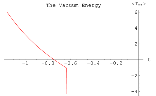
Figure 2: The abrupt drop of the vacuum energy happens at $t=t_{2}$. This figure is plotted for the same constants in Fig. 1.

Finally, as for the induced vacuum energy (18), it is constant, which is explicitly written as

$$<T_{\pm\pm}> = -2\kappa P_{\Omega_{0}}^{2}\left(1+\frac{P_{\chi_{0}}}{P_{\Omega_{0}}}\right)$$ (37)

$$= -2\kappa P_{\Omega_{0}}^{2}\left(1+\tanh(2\kappa\theta_{2}t_{2})\right),$$

for $t>t_{2}$ by the use of Eq. (35), which is negative energy density. On the other hand, the induced vacuum energy for $t_{1}<t<t_{2}$ is obtained by eliminating the constant $\beta$ in Eq. (30) in terms of Eq. (32),

$$<T_{\pm\pm}>=-\kappa P_{\Omega_{0}}{\rm sech}(2\kappa\theta_{2}t_{2})\left[\kappa\theta_{2}\sinh(2\kappa\theta_{2}t)+2P_{\Omega_{0}}{\rm sech}(2\kappa\theta_{2}t_{2})e^{2\kappa\theta_{2}t}\cosh(2\kappa\theta_{2}t)\right].$$ (38)

Note that it is mostly positive where it becomes negative just before $t_{2}$. The vacuum energy is jumped down as seen from Eqs. (37) and (38), which is essentially due to our assumption of the noncommutativity using the abrupt step functions.

The noncommutativity represented by modified Poisson brackets gives the phase changing from the decelerating to the accelerating phase, however, the acceleration does not end and it eventually diverges. Therefore, the noncommutativity should be terminated at a certain time after phase changing. So, the finite accelerating region from the commutativity is patched up in order to avoid the divergent acceleration. Unfortunately, the duration of the noncommutativity is expressed by the simplified step function, which yields the jumped down behavior of the energy momentum tensors. Even in this simplified assumption for the noncommutative parameter, $\Omega$ and $\chi$ in Eqs. (32)-(35) are continuous at the intersection point up to their time derivatives. These requirements show that the dilaton field in Eq. (27) is continuous up to their derivative and subsequently the metric or scale factor in Eq. (28) is too. On the other hand, the continuity of the scalar curvature guarantees the continuity of the second derivatives of the metric since it is written as $R=8e^{-2\rho}\partial_{+}\partial_{-}\rho$ in two-dimensions. Of course, the curvature scalar is not analytic but continuous. Our matching condition does not imply the analyticity of the curvature scalar but the continuity of them. We expect a smooth matching may be possible if we take a smooth noncommutativity parameter, which has not been studied in this work.

The accelerating cosmology naturally appears in the semi-classically quantized dilaton gravity called the BPP model in the black hole model bpp . In this cosmological model, the dilaton driven acceleration is not a weird phenomenon in that the dilaton field plays an ghost or phantom-like role in terms of its wrong sign kinetic term in our starting action, which is on the contrary to the conventional Einstein theory which predicts the deceleration with the ordinary matter. These two drastically different contents are incorporated in the present model through the dilaton driven acceleration and the vacuum energy driven deceleration. The latter in Eq. (30) is mostly positive, it behaves as an ordinary matter which contributes deceleration of the universe.

In some sense, the dark energy is originated from the the dilaton in our model and the description of the decelerating universe becomes impossible, so that we have considered the quantum-mechanically induced normal energy which partially compensates the dark energy in the past. In fact, to obtain the nontrivial energy-momentum tensor, we have introduced the noncommutative algebra only for the early time. This technical point is intuitively compatible with our feeling that the noncommutativity is natural to apply the early universe instead of the present large universe.

At first sight, our starting semiclassical action seems to be quantized one more, however, this is not the case since the modified Poisson brackets are simply the counterpart of the conventional Poisson brackets which are not quantum commutators. In the Hamiltonian formulation using the usual Poisson brackets, the Hamiltonian equations of motion written in the form of the first order with respect to the time can be classically solved, then the solutions are exactly same with those of the original Euler-Lagrangian equations of motion unless we regard the fields as operators. If the fields had been taken as operators by decomposing the positive and the negative frequency modes along with the normal ordering, then that would be the quantization of a quantization. But our modified Poisson brackets just modify the conventional (semiclassical) Hamiltonian equations of motion, which still result in the semiclassical solutions, of course, they are theta dependent due to the modification of the Poisson brackets. Unfortunately, in our model, we do not know how to obtain theta dependent Euler-Lagrangian equations of motion directly from the Lagrangian. There may be such a nice Lagrangian formulation depending on models case by case as very slowly moving point particle in the constant magnetic field or D-branes in a constant Neveu-Schwarz two form field studied originally in Ref. [20]. On the other hand, our theta-independent classical and semiclassical action do not give the desired phase change of acceleration. Thus, the purpose of this modification is to find whether the phase changing solution can be obtained or not. So, our solution is not the quantized one of the semiclassically quantized model but the theta dependent semiclassical solution. These theta dependent Poisson brackets can be applied at the various level of quantization. Secondly, the reason why we applied the modified theta dependent Poisson brackets to the semiclassical action (4) instead of the original classical action (2) is to use the local undetermined function $t_{\pm}$ in the semiclassical version which is related to the vacuum state of the quantized matters. It was firstly introduced in Ref. [6] to determine the geometry of the black hole, which is absent in the classical theory. The phase change is essentially related to the energy momentum tensors, and the fine-tuned classical energy-momentum tensors may give the phase changing solution, however, it seems to be more or less ad hoc. However, our model is based on the fact that the necessary energy and pressure in order for the phase change come from the part of quantized matters through $t_{\pm}$ in the semiclassical theory.

In our model, there is an initial singularity at $t_{1}$, which may be removable in the other quantization scheme. Unfortunately, what is worse, this model does not contain the transition from the inflationary era to the decelerating phase in the early universe. So, it might be interesting to study these problems in this scheme.

In summary, our model does not describe our whole genuine universe, though, it seems to be meaningful to suggest an alternative to show the phase transition from the deceleration universe to the accelerating universe chronologically through the analytic model.

- (1) S. Perlmutter et al., Astrophys. J. 517 (1999) 565 [astro-ph/9812133].
- (2) D. N. Spergel et al., Astrophys. J. Suppl. 148 (2003) 175 [astro-ph/0302209].
- (3) R. R. Caldwell, Phys. Lett. B 545 (2002) 23 [astro-ph/9908168].
- (4) S. M. Carroll, A. D. Felice, V. D., D. A. Easson, M. Trodden, and M. S. Turner, Phys. Rev. D 71(2005) 063513 [astro-ph/0410031].
- (5) T. Biswas, R. Brandenberger, A. Mazumdar, and T. Multamaki, Current acceleration from dilaton and stringy cold dark matter, hep-th/0507199.
- (6) S. Nojiri and S. D. Odintsov, Phys. Rev. D 70 (2005) 103522 [hep-th/0408170].
- (7) H. Kim, H. W. Lee, and Y. S. Myung, Phys. Lett. B 632 (2006) 605 [gr-qc/0509040].
- (8) H. Wei and R.-G. Cai, Phys. Rev. D 73 (2006) 083002 [astro-ph/0603052].
- (9) R. B. Mann and S. F. Ross, Phys. Rev. D 47 (1993) 3312 [hep-th/9206022]; K. C. K. Chan and R. B. Mann, Class. and Quant. Grav. 10 (1993) 913 [gr-qc/9210015].
- (10) M. Gasperini and G. Veneziano, Phys. Lett. B 387 (1996) 715 [hep-th/9607126].
- (11) S. J. Rey, Phys. Rev. Lett. 77 (1996) 1929 [hep-th/9605176].
- (12) S. K. Bose and S. Kar, Phys. Rev. D 56 (1997) 4444 [hep-th/9705061].
- (13) W. Kim and M. S. Yoon, Phys. Lett. B 423 (1998) 231 [hep-th/9706154].
- (14) W. Kim and M. S. Yoon, Phys. Rev. D 58 (1998) 084014 [hep-th/9803081].
- (15) M. H. Christmann, F. P. Devecchi, G. M. Kremer, and C. M. Zanetti, Europhys. Lett. 67 (2004) 728 [gr-qc/0407029].
- (16) C. G. Callan, S. B. Giddings, J. A. Harvey, and A. Strominger, Phys. Rev. D 45 (1992) 1005 [hep-th/9111056].
- (17) J. G. Russo, L. Susskind, and L. Thorlacius, Phys. Rev. D 46 (1992) 3444 [hep-th/9206070].
- (18) S. K. Bose, L. Parker, and Y. Peleg, Phys. Rev. Lett. 76 (1996) 861 [gr-qc/9508027].
- (19) W. Kummer and D. Vassilevich, Phys. Rev. D 60 (1999) 084021 [hep-th/9811092].
- (20) N. Seiberg and E. Witten, J. High Energy Phys. 09 (1999) 032 [hep-th/9908142].
- (21) G. D. Barbosa and N. Pinto-Neto, Phys. Rev. D 70 (2004) 103512 [hep-th/0407111].
- (22) D. Vassilevich, Stability of a noncommutative Jackiw-Teitelboim gravity, hep-th/0602095.
- (23) W. Kim and J. J. Oh, Mod. Phys. Lett. 15 (2000) 1597 [hep-th/9911085].
- (24) A. Bilal and C. Callan, Nucl. Phys. B 394 (1993) 73 [hep-th/9205089].
- (25) A. Bilal and I. I. Kogan, Phys. Rev. D 47 (1993) 5408 [hep-th/9301119].