Semiclassical approach to the decay of protons in circular motion under the influence of gravitational fields

Abstract

We investigate the possible decay of protons in geodesic circular motion around neutral compact objects. Weak and strong decay rates and the associated emitted powers are calculated using a semi-classical approach. Our results are discussed with respect to distinct ones in the literature, which consider the decay of accelerated protons in electromagnetic fields. A number of consistency checks are presented along the paper.

I Introduction

It is well known that according to the particle standard model inertial protons are stable. However, this is not so if the proton is under the influence of some external force because in this case the accelerating agent can provide the required extra energy, which allows the proton to decay. To the best of our present knowledge, the first ones to consider the decay of accelerated protons and similar processes as

$$p^{+}\stackrel{{\scriptstyle a}}{{\to}}p^{+}\,\pi^{0}\,,$$ (1)

were Ginzburg and Zharkov GZ -Zhar . In Ref. GZ the proton is described by a classical current with a well defined trajectory while the pion is field quantized. This approach is accurate in the no-recoil regime, i.e. when the relevant parameter $\chi\equiv a/m_{p}$ involving the $p^{+}$’s proper acceleration $a$ and mass $m_{p}$ is less than unity. At the same time, Zharkov Zhar (see also Ref. R for a recent review) investigated the process

$$p^{+}\stackrel{{\scriptstyle A_{\mu}}}{{\to}}p^{+}\,\pi^{0}$$ (2)

and the strong and weak proton decays

$$p^{+} \stackrel{{\scriptstyle A_{\mu}}}{{\to}} n^{0}\,\pi^{+}\,,$$ (3)

$$p^{+} \stackrel{{\scriptstyle A_{\mu}}}{{\to}} n^{0}\,e^{+}\,\nu\,,$$ (4)

respectively, in the presence of an electromagnetic field $A_{\mu}$, where all particles are field quantized. For this purpose, it was used the comprehensive formalism developed by Nikishov and Ritus NR (see also ritus69 ), which allows one to investigate quantum processes in such a background. The study of particle processes in the presence of strong electromagnetic fields should be important to the analysis of certain aspects of high energy cosmic ray physics produced in pulsars and magnetars. In such intense magnetic fields ($H\sim 10^{12}-10^{17}$ G) the strong coupling of protons and neutrons with mesons can generate $\rho$’s and $\pi$’s with a non negligible intensity TK -berez .

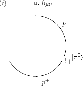
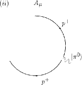
Figure 1: The process $p^{+}\to p^{+}\,\pi^{0}$ is represented in the presence of background gravitational ($h_{\mu\nu}$) and electromagnetic ($A^{\mu}$) fields. In the proper regime, this process can be well described in both backgrounds by the classical current approach, where the proton is assumed to have a well defined worldline with acceleration $a$ and the pion is field quantized. Notice the similarity of the proton behavior in $(i)$ and $(ii)$.

In the proper regime (i.e. where backreaction effects are not important), the reaction rate associated with processes (1) when the $p^{+}$ is in circular motion and (2) when it is under the influence of a magnetic field coincide. Notwithstanding, this is not so for the processes (3)-(4), and

$$p^{+} \stackrel{{\scriptstyle a}}{{\to}} n^{0}\,\pi^{+}\,,$$ (5)

$$p^{+} \stackrel{{\scriptstyle a}}{{\to}} n^{0}\,e^{+}\,\nu\,,$$ (6)

respectively (where the $p^{+}-n^{0}$ are described by a classical current). This is a consequence of the fact that in the classical current approach both, proton and neutron, are usually assumed to follow the same trajectory in contrast with what really happens in the presence of a background magnetic field (notice the difference between Fig. 1, and Figs. 2 and 3).

This raises the question about what is the physical situation simulated by the classical current method when applied to the processes (5) and (6), where one considers that only mesons and leptons are field quantized. Once protons and neutrons are described by a common current, one should look for a situation where they are mainly undistinguishable. This is what happens in gravitational fields according to the equivalence principle. (For early and recent investigations on geodesic synchrotron radiation from classical currents see Refs. Misneretal and Lemosetal , respectively.) As a consequence, processes (5) and (6) should represent fairly well the strong and weak conversion of protons into neutrons when they orbit chargeless compact objects provided that the back reaction on the neutron is negligible. This is what we are going to investigate in this paper.

In our procedure, we take into account the proton-neutron mass difference, by introducing a semiclassical rather than classical current. We will be following Ref. MV , where a semiclassical current was successfully used to model the decay of linearly accelerated protons in the study of the Fulling-Davies-Unruh effect FDU . The current is “classical” in the sense that the proton-neutron is associated with a well defined worldline and “quantum” in the sense that it behaves as a two-level quantum system.

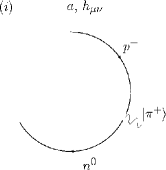
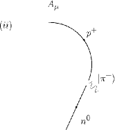
Figure 2: The process $p^{+}\to n^{0}\,\pi^{+}$ is represented in the presence of background gravitational ($h_{\mu\nu}$) and electromagnetic ($A^{\mu}$) fields. Only in the first case it can be well described, in the proper regime, by the classical current approach labeled by the nucleons’ proper acceleration $a$. Notice the difference of the proton-neutron behavior in $(i)$ and $(ii)$.

(A simplified related calculation, where all particles are treated as scalars can be found in Ref. M .) The calculation is performed in Minkowski spacetime and the gravitational field is described by a Newtonian-like central force.

There is also an important difference concerning the proton decay when it is under the influence of a gravitational field rather than of a magnetic one, which is worthwhile to call the attention. The physical scale for the proton decay is given by its proper acceleration $a$. Because of the pion mass, process (6) dominates over process (5) in the region $m_{e}+\Delta\mu<a<m_{\pi}+\Delta\mu$ and because of the magnitude of the strong coupling constant, process (5) dominates over process (6) in the region $a>m_{\pi}+\Delta\mu$, where $\Delta\mu=m_{n}-m_{p}$. Now, in the presence of a magnetic field $H$, the proper acceleration of a proton in circular motion can be written as $a=\gamma eH/m_{p}$, where $\gamma=E/m_{p}$ is the usual relativistic factor given by the ratio of the proton’s energy and mass. In the region $a>m_{\pi}+\Delta\mu$, the strong process dominates over electromagnetic processes and energy degradation through photon emission does not play any relevant role. This is not so, however, in the region $m_{e}+\Delta\mu<a<m_{\pi}+\Delta\mu$, where electromagnetic processes dominate over the weak one and much of the proton’s energy $E$ can be carried away by the photons, driving its acceleration below the threshold $m_{e}+\Delta\mu$. (Recall that $\gamma$ is proportional to $E$.) The situation is quite different in a gravitational field. Assuming Minkowski space, the proper acceleration $a=R\Omega^{2}\gamma^{2}$ of a proton in circular orbit with radius $R$ and angular velocity $\Omega$ around a compact object with mass $M$ can be written as $a=(GM\Omega^{4})^{1/3}/(1-(GM\Omega)^{2/3})$, where we have used the Newtonian gravity relation $R^{3}\Omega^{2}=GM$. Then, as the orbiting proton emits photons descending to a more internal orbit with larger $\Omega$, its proper acceleration tends to increase rather than to decrease, in contrast to the electromagnetic case. Whether or not a proton decays along its inspiraling trajectory will depend on the mass of the central object and other details, which will be discussed further.

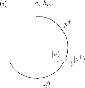
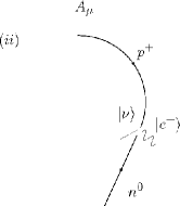
Figure 3: The process $p^{+}\to n^{0}\,e^{+}\,\nu$ is represented in the presence of background gravitational ($h_{\mu\nu}$) and electromagnetic ($A^{\mu}$) fields. Analogously to the previous figure, only the first case can be well described, in the proper regime, by the classical current approach.

Now one may wonder how accurate can be our results when applied to quite strong gravitational fields. In principle, an exact calculation would require that we take into account the spacetime curvature in the particle field quantization. However, as it was shown in Refs. CHM and CCMM the results obtained assuming a full curved spacetime ruled by Einstein equations and a flat background endowed with a Newtonian attraction force should not differ by more than 20%-30% up to the inner stable circular orbit of a static black hole. This is going to suffice for our purposes.

The paper is organized as follows: In Sec. II we present the semiclassical current formalism. In Sec. III we evaluate the scalar and fermion emission rates for a uniformly swirling current. In Sec. IV we evaluate the corresponding radiated powers. In Sec. V we use the previous results to analyze the decay of protons orbiting chargeless compact objects. Consistency checks for our formulas are presented. We dedicate Sec. VI to our final discussions. We assume Minkowski spacetime with metric components $\eta_{\mu\nu}={\rm diag}(+1,-1,-1,-1)$ associated with the usual inertial coordinates $(t,{\bf x})$ and adopt natural units $c=\hbar=1$ throughout this paper unless stated otherwise.

II Semiclassical current formalism

Let us consider the following class of processes

$$p_{1}\; \to \;p_{2}\;g\;,$$ (7)

$$p_{1}\; \to \;p_{2}\;f_{1}\;\bar{f}_{2}\;,$$ (8)

where a scalar $g$ or a fermion-antifermion pair $f_{1}$-$\bar{f}_{2}$ are emitted as the particle $p_{1}$ evolves into $p_{2}$. The $g$, $f_{1}$, $\bar{f}_{2}$, $p_{1}$ and $p_{2}$’s rest masses are $m$, $m_{1}$, $m_{2}$, $M_{1}$ and $M_{2}$, respectively. We will be interested here in cases where $m,m_{1},m_{2}\ll M_{1},M_{2}$. The particle emission will be assumed not to change significantly the four-velocity of $p_{2}$ with respect to $p_{1}$. This is called “no-recoil condition”, which is verified when the momentum of the emitted particles with respect to the instantaneously inertial rest frame lying at $p_{1}$ satisfies $|{\bf k}_{\rm rf}|\ll M_{1},\;M_{2}$. Because $m,m_{1},m_{2}\ll M_{1},M_{2}$, this implies that the energy of each emitted particle satisfies ${\omega}_{\rm rf}\ll M_{1},\;M_{2}$. As the typical energy $\omega_{\rm rf}$ of the emitted particles is of the order of $p_{1}$’s proper acceleration $a\equiv\sqrt{|a_{\mu}a^{\mu}|}$, the no-recoil condition can be recast in the frame independent form VM3

$$a\ll M_{1},\;M_{2}\;.$$ (9)

The particles $p_{1}$ and $p_{2}$ will be seen as distinct energy eigenstates $|p_{1}\rangle$ and $|p_{2}\rangle$, respectively, of a two-level system. The associated proper Hamiltonian $\hat{H}_{0}$ of the particle system satisfies, thus,

$$\hat{H}_{0}\;|p_{j}\rangle=M_{j}\;|p_{j}\rangle\;,\;\;j=1,2\;.$$ (10)

We shall describe our pointlike particle system $p_{1}$-$p_{2}$ in the process (7) by the semiclassical scalar source

$$\hat{j}(x)=[\hat{q}(\tau)/u^{0}(\tau)]\;\delta^{3}[{\bf x}-{\bf x}(\tau)]$$ (11)

and in the process (8) by the vector current

$$\hat{j}^{\mu}(x)=[\hat{q}(\tau)\;u^{\mu}(\tau)/u^{0}(\tau)]\;\delta^{3}[{\bf x}-{\bf x}(\tau)]\;.$$ (12)

Here $x^{\mu}(\tau)$ is the classical world line parametrized by the proper time $\tau$ associated with $p_{1}$-$p_{2}$, $u^{\mu}(\tau)\equiv dx^{\mu}/d\tau$ is the corresponding four-velocity, and $\hat{q}(\tau)\equiv e^{i\hat{H}_{0}\tau}\hat{q}_{0}e^{-i\hat{H}_{0}\tau}$, where $\hat{q}_{0}$ is a self-adjoint operator evolved by the one-parameter group of unitary operators $\hat{U}(\tau)=e^{-i\hat{H}_{0}\tau}$.

The emitted scalar $g$ in the process (7) is associated with a complex Klein-Gordon field

$$\hat{\Phi}(x)=\int d^{3}{\bf k}\left[\hat{a}_{{\bf k}}\phi^{(+\omega)}_{{\bf k}}(x)+\hat{c}^{\dagger}_{{\bf k}}\phi^{(-\omega)}_{-{\bf k}}(x)\right]\;,$$ (13)

while the emitted fermions $f_{1}-\bar{f}_{2}$ in the process (8) are associated with the fermionic one

$$\hat{\Psi}_{i}(x)=\sum_{\sigma=\pm}\int d^{3}{\bf k}_{i}\left[\hat{b}_{{\bf k}_{i}\sigma}\psi^{(+\omega_{i})}_{{\bf k}_{i}\sigma}(x)+\hat{d}^{\dagger}_{{\bf k}_{i}\sigma}\psi^{(-\omega_{i})}_{-{\bf k}_{i}-\sigma}(x)\right]\;,$$ (14)

where $i=1,2$ labels the two fermions. Here $\hat{a}_{{\bf k}}\;(\hat{a}^{\dagger}_{{\bf k}})$, $\hat{b}_{{\bf k}_{i}\sigma}\;(\hat{b}^{\dagger}_{{\bf k}_{i}\sigma})$, $\hat{c}_{{\bf k}}\;(\hat{c}^{\dagger}_{{\bf k}})$ and $\hat{d}_{{\bf k}_{i}\sigma}\;(\hat{d}^{\dagger}_{{\bf k}_{i}\sigma})$ are annihilation (creation) operators of scalars, fermions, antiscalars and antifermions, respectively, with three-momentum ${\bf k}=(k^{x},k^{y},k^{z})$ and energy $\omega=\sqrt{{\bf k}^{2}+m^{2}}$ for the scalar, and ${\bf k}_{i}=(k_{i}^{x},k_{i}^{y},k_{i}^{z})$ and $\omega_{i}=\sqrt{{\bf k}_{i}^{2}+m_{i}^{2}}$ for the fermions. $\phi^{(\pm\omega)}_{\bf k}$ and $\psi^{(\pm\omega_{i})}_{{\bf k}_{i}\sigma}$ are positive $[(+\omega),(+\omega_{i})]$ and negative $[(-\omega),(-\omega_{i})]$ frequency solutions of the Klein-Gordon $(\Box-m^{2})\phi^{(\pm\omega)}_{\bf k}=0$ and Dirac $(i\gamma^{\mu}\partial_{\mu}-m_{i})\psi^{(\pm\omega_{i})}_{{\bf k}_{i}\sigma}=0$ equations, respectively, where $\sigma$ labels the fermion polarization.

Next, we minimally couple the fields to our semiclassical source (11) and current (12) according to the actions IZ -CQ

$$\hat{S}_{I}^{(s)}=\int d^{4}x\;\hat{j}(x)\left[\hat{\Phi}(x)+\hat{\Phi}^{\dagger}(x)\right]$$ (15)

for the scalar and

$$\hat{S}_{I}^{(f)} = \int d^{4}x\;\hat{j}_{\mu}(\hat{\bar{\Psi}}_{1}\gamma^{\mu}(c_{V}-c_{A}\gamma^{5})\hat{\Psi}_{2}$$ (16)

$$+ \hat{\bar{\Psi}}_{2}\gamma^{\mu}(c_{V}-c_{A}\gamma^{5})\hat{\Psi}_{1})$$

for the fermionic cases, (7) and (8), respectively, where $\hat{\bar{\Psi}}=\hat{\Psi^{\dagger}}\gamma^{0}$ and $c_{V}=c_{A}=1$ in the processes here analyzed.

The transition amplitudes at the tree level for the processes (7) and (8) are given by

$${\cal A}_{{\bf k}}=\;\langle p_{2}|\otimes\langle{g}_{{\bf k}}|\;\hat{S}_{I}^{(s)}\;|0\rangle\otimes|p_{1}\rangle\;,$$ (17)

and

$${\cal A}^{\sigma_{1}\sigma_{2}}_{{\bf k}_{1}{\bf k}_{2}}=\;\langle p_{2}|\otimes\langle{f_{1}}_{{\bf k}_{1}\sigma_{1}},\bar{f_{2}}_{{\bf k}_{2}\sigma_{2}}|\;\hat{S}_{I}^{(f)}\;|0\rangle\otimes|p_{1}\rangle\;,$$ (18)

respectively. The differential transition probabilities are

$$\frac{d{\cal P}_{s}^{p_{1}\to p_{2}}}{d^{3}{\bf k}} = |{\cal A}_{{\bf k}}|^{2}$$ (19)

$$= \frac{G_{\rm eff}^{(s)2}}{2(2\pi)^{3}\omega}\int_{-\infty}^{+\infty}\!\!\!\!d\tau\int_{-\infty}^{+\infty}\!\!\!\!d\tau^{\prime}\exp\{i\Delta\mu(\tau-\tau^{\prime})$$

$$+ik^{\lambda}[x(\tau)-x(\tau^{\prime})]_{\lambda}\}$$

and

$$\frac{d{\cal P}_{f}^{p_{1}\to p_{2}}}{d^{3}{\bf k}_{1}d^{3}{\bf k}_{2}} = \sum_{\sigma_{1}=\pm}\sum_{\sigma_{2}=\pm}|{\cal A}^{\sigma_{1}\sigma_{2}}_{{\bf k}_{1}{\bf k}_{2}}|^{2}$$ (20)

$$= \!\!\!\frac{2\;G_{\rm eff}^{(f)2}}{(2\pi)^{6}\omega_{1}\omega_{2}}\!\int_{-\infty}^{+\infty}\!\!\!\!\!d\tau\int_{-\infty}^{+\infty}\!\!\!\!\!d\tau^{\prime}\exp\{i\Delta\mu(\tau-\tau^{\prime})$$

$$+ i(k_{1}+k_{2})^{\lambda}[x(\tau)-x(\tau^{\prime})]_{\lambda}\}$$

$$\times \!\!\!\{2k_{1}^{(\mu}k_{2}^{\nu)}u_{\mu}(\tau)u_{\nu}(\tau^{\prime})-k_{1}^{\alpha}{k_{2}}_{\alpha}u^{\mu}(\tau)u_{\mu}(\tau^{\prime})$$

$$+ i\epsilon^{\mu\nu\alpha\beta}k_{1\alpha}k_{2\beta}u_{\mu}(\tau)u_{\nu}(\tau^{\prime})\}\;,$$

accordingly, where $\epsilon^{\mu\alpha\nu\beta}$ is the totally skew-symmetric Levi-Civita pseudo-tensor (with $\epsilon^{0123}=-1$), $k_{1}^{(\mu}k_{2}^{\nu)}\equiv(k_{1}^{\mu}k_{2}^{\nu}+k_{1}^{\nu}k_{2}^{\mu})/2$, $\Delta\mu\equiv M_{2}-M_{1}$ and $G_{\rm eff}^{(s),(f)}\equiv|\langle p_{2}|\hat{q}_{0}|p_{1}\rangle|$ are the effective coupling constants for the scalar $(s)$ and fermionic $(f)$ channels.

III Emission rates

The world line of a particle with uniform circular motion with radius $R$ and angular velocity $\Omega$ as defined by laboratory observers at rest in an inertial frame with coordinates $(t,{\bf x})$, is

$$x^{\mu}(\tau)=(t\;,\;R\cos(\Omega t)\;,\;R\sin(\Omega t)\;,\;0)$$ (21)

and the corresponding four-velocity is

$$u^{\mu}(\tau)=\gamma\,(1\;,\;-R\Omega\sin(\Omega t)\;,\;R\Omega\cos(\Omega t)\;,\;0)\;,$$ (22)

where $\gamma\equiv(1-R^{2}\Omega^{2})^{-1/2}=\rm const$ is the Lorentz factor ($v\equiv R\Omega<1$), $t=\gamma\tau$, and $a=\sqrt{-a_{\mu}a^{\mu}}=R\,\Omega^{2}\gamma^{2}$ is the proper acceleration. Let us calculate now separately the scalar and fermionic emission rates associated with processes (7) and (8), respectively.

III.1 Scalar case

First, let us analyze the process (7). In order to decouple the integrals in Eq. (19), we define new coordinates,

$$\sigma\equiv\gamma({\tau-\tau^{\prime}})/{2}\;\;\;\;{\rm and}\;\;\;\;s\equiv\gamma({\tau+\tau^{\prime}})/{2}\;,$$ (23)

and perform the change in the momentum variable

$$k^{\mu}\mapsto{\widetilde{k}}^{\mu}=({\widetilde{\omega}}\;,{\widetilde{\bf k}})\;,$$ (24)

where

$${\widetilde{\omega}}\; = \omega\;,$$

$${\widetilde{k}^{x}} = k^{x}\cos(\Omega s)+k^{y}\sin(\Omega s)\;,$$

$${\widetilde{k}^{y}} = -k^{x}\sin(\Omega s)+k^{y}\cos(\Omega s)\;,$$

$${\widetilde{k}^{z}} = k^{z}\;,$$

which consists of a rotation by an angle $\Omega s$ around the $k^{z}$ axis. Hence, we obtain from Eq. (19) the following transition rate per momentum-space element for the emitted scalar:

$$\frac{d{\cal R}_{s}^{p_{1}\to p_{2}}}{d^{3}{\widetilde{\bf k}}} = \frac{\;\;G_{\rm eff}^{(s)2}}{(2\pi)^{3}{2\gamma^{2}\widetilde{\omega}}}\int_{-\infty}^{+\infty}d\sigma\;\exp[i(\Delta\mu\sigma/\gamma$$ (25)

$$+ \widetilde{k}^{\mu}X_{\mu}(\sigma))]\;,$$

where ${\cal R}_{s}^{p_{1}\to p_{2}}\equiv{d{\cal P}^{p_{1}\to p_{2}}}/{ds}\;$ is the transition probability per laboratory time and

$$X^{\mu}(\sigma)\equiv(\sigma\,,\,0\,,\,2R\sin(\Omega\sigma/2)\,,\,0)\;.$$ (26)

In order to calculate the transition rate

$${\cal R}_{s}^{p_{1}\to p_{2}}\equiv\int d^{3}\widetilde{\bf k}\;\frac{d{\cal R}_{s}^{p_{1}\to p_{2}}}{d^{3}\widetilde{\bf k}}\;,$$ (27)

we use Eq. (25) and obtain

$${\cal R}_{s}^{p_{1}\to p_{2}}=\frac{G_{\rm eff}^{(s)2}}{2\;\gamma^{2}\;(2\pi)^{3}}\int_{-\infty}^{+\infty}d\sigma\;e^{i\;\Delta\mu\;\sigma/\gamma}I(\sigma)\;,$$ (28)

where

$$I(\sigma)\equiv\int d^{3}\widetilde{\bf k}\frac{e^{i\;\widetilde{k}^{\lambda}X_{\lambda}}}{\widetilde{\omega}}$$ (29)

and $\widetilde{\omega}=\sqrt{\widetilde{\bf k}^{2}+m^{2}}$. In order to integrate Eq. (29), we introduce spherical coordinates in the momenta space $({\widetilde{k}}\in{\rm R}^{+},{\widetilde{\theta}}\in[0,\pi],{\widetilde{\phi}}\in[0,2\pi))$, where ${\widetilde{k}}^{x}={\widetilde{k}}\sin{\widetilde{\theta}}\cos{\widetilde{\phi}}$, ${\widetilde{k}}^{y}={\widetilde{k}}\sin{\widetilde{\theta}}\sin{\widetilde{\phi}}$, and ${\widetilde{k}}^{z}={\widetilde{k}}\cos{\widetilde{\theta}}$. By doing so, we obtain

$$I(\sigma)=\frac{4\pi}{|{\bf X}|}\int_{m}^{+\infty}d{\widetilde{\omega}}e^{i{\widetilde{\omega}}X^{0}}\sin\left[\sqrt{{\widetilde{\omega}}^{2}-m^{2}}\;|{\bf X}|\right]\;,$$

where $|{\bf X}|\equiv\sqrt{-X_{i}X^{i}\,}$. Next, by redefining the frequency variable as $\widetilde{\omega}\equiv m\cosh\xi$, we obtain

$$I(\sigma)=\frac{-2\pi im}{|{\bf X}|}\int_{-\infty}^{+\infty}d\xi e^{im(X^{0}\cosh\xi+|{\bf X}|\sinh\xi)}\sinh\xi.$$

Now, we perform the change of variable $\xi\mapsto\eta\equiv e^{\xi}$, leading to

$$I(\sigma)=\frac{i\pi m}{|{\bf Y}|}\int_{0}^{+\infty} d\eta(\eta^{-2}-1)\exp\left[\frac{im(Y^{0}+|{\bf Y}|)\eta}{2}\right.$$ (30)

$$\left.+\frac{im(Y^{0}-|{\bf Y}|)}{2\eta}\right]\;,$$

where we have introduced a small positive regulator $\epsilon>0$ in the integral as follows:

$$X^{\mu}\mapsto Y^{\mu}=(X^{0}+i\epsilon,X^{1},X^{2},X^{3})\;.$$ (31)

(Note that $|{\rm Re}(Y^{0})|=|X^{0}|>|{\bf X}|=|{\bf Y}|$.) Then, by using expressions (3.471.11) and (8.484.1) of Ref. GR , we obtain

$$I(\sigma)=\frac{-2\,\pi^{2}\,i\,\,m\,{\rm sign}(\sigma)}{\sqrt{Y_{\mu}Y^{\mu}\,}}H_{1}^{(1)}\left({\rm sign}(\sigma)m\sqrt{Y_{\mu}Y^{\mu}\,}\right)\;,$$ (32)

where $H^{(1)}_{1}(z)$ is the Hankel function of the first kind. As a result, by making the variable change $\sigma\mapsto\lambda\equiv-a\sigma/\gamma$ and by defining $Z^{\mu}\equiv(a/\gamma)Y^{\mu}$, the transition rate (28) can be cast in the form

$${\cal R}_{s}^{p_{1}\to p_{2}}=\frac{-iG_{\rm eff}^{(s)2}\widetilde{m}^{2}a}{8\pi\,\gamma}\int_{-\infty}^{+\infty}d\lambda\;e^{-i\;\widetilde{\Delta\mu}\,\lambda}\frac{H_{1}^{(1)}(z)}{z}\;,$$ (33)

where we have defined $\widetilde{m}\equiv m/a$, $\widetilde{\Delta\mu}\equiv\Delta\mu/a$, $\epsilon^{\prime}\equiv a\epsilon/\gamma\ll 1$, $z\equiv-\widetilde{m}\gamma{\rm sign}(\lambda)\sqrt{Z_{\lambda}Z^{\lambda}\,}$, and where

$$Z^{\mu}=(-\lambda+i\epsilon^{\prime},0,-(2Ra/\gamma)\sin(\Omega\lambda\gamma/2a),0).$$ (34)

Eq. (33) is our general formula for the transition rate per laboratory time.

In the physically interesting regime, where $\widetilde{m}\ll 1$ it can be integrated using the following expansion for the Hankel function GR :

$$H_{1}^{(1)}(z)\approx-\frac{2i}{\pi z}+{\cal O}(z\ln z)\;\;{\rm for}\;\;|z|\ll 1\;.$$ (35)

We note that for large enough $|\lambda|$, $|z|>1$, Eq. (35) ceases to be a good approximation. [For instance, for $\gamma^{2}\gg 1/\widetilde{m}\gg 1$, we have that $|z|>1$ for $|\lambda|\geq 1/\sqrt{12\widetilde{m}\,}$, while for $1/\widetilde{m}\gg\gamma^{2}\gg 1$, we have that $|z|>1$ for $|\lambda|\geq 1/(\gamma\widetilde{m})$.] Notwithstanding, this is not important because the error committed in this region is small to affect the final result provided that $\widetilde{m}\ll 1$. Hence we write Eq. (33) for $\widetilde{m}\ll 1$ in the form

$${\cal R}_{s}^{p_{1}\to p_{2}}\approx\frac{-G_{\rm eff}^{(s)2}a}{4\pi^{2}\gamma^{3}}\int_{-\infty}^{+\infty}d\lambda\;\frac{e^{-i\;\widetilde{\Delta\mu}\,\lambda}}{(Z^{\lambda}Z_{\lambda})}\;,$$ (36)

where

$$Z_{\lambda}Z^{\lambda}=(\lambda-i\epsilon^{\prime})^{2}-(2Ra/\gamma)^{2}\sin^{2}(\Omega\lambda\gamma/2a)\,.$$ (37)

In order to solve this integral, we expand $Z^{\lambda}Z_{\lambda}$ for relativistic swirling particles T , i.e., $\gamma\gg 1$ (recall that $R=v^{2}\gamma^{2}/a$, $\Omega=a/(v\gamma^{2})$, and $v=\sqrt{1-\gamma^{-2}}$):

$$Z_{\lambda}Z^{\lambda} \approx \frac{1}{12\,\gamma^{2}}(\lambda+i\sqrt{3}A_{+})(\lambda+i\sqrt{3}A_{-})(\lambda-i\sqrt{3}B_{+})$$ (38)

$$\times(\lambda-i\sqrt{3}B_{-})\;,$$

where

$$A\mp\equiv 1\mp\sqrt{1+2\widetilde{\epsilon}/\sqrt{3}}$$

and

$$B\mp\equiv 1\mp\sqrt{1-2\widetilde{\epsilon}/\sqrt{3}}$$

with $\widetilde{\epsilon}\ll 1$. For $|\lambda|\gtrsim 2v\gamma$, where the expansion ceases to be a good approximation, the integral contributes very little again and, thus, will not have any major influence in the final result. Thus, the integral in Eq. (36) can be rewritten in the complex plane:

$${\cal R}_{s}^{p_{1}\to p_{2}}\approx\frac{-G_{\rm eff}^{(s)2}a}{4\pi^{2}\gamma^{3}}\oint_{C}d\lambda\;\frac{e^{-i\;\widetilde{\Delta\mu}\,\lambda}}{Z^{\lambda}Z_{\lambda}}\;,$$ (39)

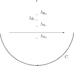
Figure 4: The integration path in complex plane. The $\lambda_{A\pm,B\pm}$ refers to the poles for each of the terms in parentheses of the Eq. (38).

where the complex integration path $C$ is clockwise oriented ($C\equiv(-L,L)\cup\{L\;e^{i\theta},\theta\in[-\pi,0]\}\,,L\to\infty$) as shown in Fig. 4. Eq. (39) can be performed, then, by using Cauchy’s residue theorem leading to

$${\cal R}_{s}^{p_{1}\to p_{2}}\approx\frac{G_{\rm eff}^{(s)2}a}{8\sqrt{3}{\pi}\gamma}\,e^{{-2\sqrt{3}\widetilde{\Delta\mu}}}\;,$$ (40)

which is valid for $\widetilde{m}\ll 1$ and $\gamma\gg 1$.

III.2 Fermionic case

Next, let us compute the transition rate associated with the fermionic $f_{1}-\bar{f}_{2}$ emission of process (8). After performing the variable changes (23) and (24), one obtains from Eq. (20),

$$\frac{d{\cal R}_{f}^{p_{1}\to p_{2}}}{d^{3}{\widetilde{\bf k}}_{1}d^{3}{\widetilde{\bf k}}_{2}}\;=\;\frac{2\;G_{\rm eff}^{(f)2}}{(2\pi)^{6}{\widetilde{\omega}}_{1}{\widetilde{\omega}}_{2}}\int_{-\infty}^{+\infty}d\sigma\;\exp[i(\Delta\mu\sigma/\gamma$$

$$+(\widetilde{k}_{1}+\widetilde{k}_{2})^{\mu}X_{\mu}(\sigma))][\,R^{2}\,\Omega^{2}({\widetilde{\omega}}_{1}{\widetilde{\omega}}_{2}-{\widetilde{k}}^{z}_{1}{\widetilde{k}}^{z}_{2})\cos(\,\Omega\sigma\,)$$

$$-R^{2}\Omega^{2}({\widetilde{k}}^{x}_{1}{\widetilde{k}}^{x}_{2}-{\widetilde{k}}^{y}_{1}{\widetilde{k}}^{y}_{2})+({\widetilde{\omega}}_{1}{\widetilde{\omega}}_{2}+{\widetilde{\bf k}}_{1}\cdot{\widetilde{\bf k}}_{2})$$

$$-\,2\,R\,\Omega\,({\widetilde{\omega}}_{1}{\widetilde{k}}^{y}_{2}+{\widetilde{\omega}}_{2}{\widetilde{k}}^{y}_{1})\cos(\,\Omega\sigma/2\,)$$

$$+\,2\,i\,R\,\Omega\,({\widetilde{\bf k}_{1}}\times{\widetilde{\bf k}_{2}})^{x}\sin(\,\Omega\sigma/2\,)$$

$$-\,i\,R^{2}\,\Omega^{2}\,({\widetilde{\omega}}_{1}{\widetilde{k}}^{z}_{2}-{\widetilde{\omega}}_{2}{\widetilde{k}}^{z}_{1})\sin(\,\Omega\sigma\,)]\;,$$ (41)

which is the laboratory transition rate per momentum-space element associated with each emitted fermion and $X^{\mu}$ is given in Eq. (26). By integrating over all momenta, the transition rate can be rewritten in a more convenient form as

$${\cal R}^{p_{1}\to p_{2}}_{f}=\frac{2\;G_{\rm eff}^{(f)2}}{(2\pi)^{6}}\int_{-\infty}^{+\infty}d\sigma\;e^{i\;\Delta\mu\;\sigma/\gamma}G_{\mu\nu}A^{\mu\nu}$$ (42)

with

$$G_{\mu\nu}\equiv-\frac{\partial I_{1}}{\partial X^{\mu}}\frac{\partial I_{2}}{\partial X^{\nu}}$$ (43)

and

$$I_{l}(\sigma)\equiv\int d^{3}\widetilde{\bf k}_{l}\frac{e^{i\;\widetilde{\bf k}_{l}^{\lambda}X_{\lambda}}}{\widetilde{\omega}_{l}}\;,$$ (44)

where the index $l=1,2$ is used to distinguish the fermion in the final state to which we are referring and $\widetilde{\omega}_{l}=\sqrt{\widetilde{\bf k}_{l}^{2}+m_{l}^{2}}$. Also

$$A_{\mu\nu}=\left[\begin{array}[]{cccc}1+R^{2}\Omega^{2}\cos(\Omega\sigma)&0&-2R\Omega\cos(\Omega\sigma/2)&-iR^{2}\Omega^{2}\sin(\Omega\sigma)\\ 0&1-R^{2}\Omega^{2}&0&0\\ -2R\Omega\cos(\Omega\sigma/2)&0&1+R^{2}\Omega^{2}&2iR\Omega\sin(\Omega\sigma/2)\\ iR^{2}\Omega^{2}\sin(\Omega\sigma)&0&-2iR\Omega\sin(\Omega\sigma/2)&1-R^{2}\Omega^{2}\cos(\Omega\sigma)\end{array}\right]\;.$$ (45)

In order to compute Eq. (44), we introduce spherical coordinates in the momenta space $({\widetilde{k}}_{l}\in{\rm R}^{+},{\widetilde{\theta}}_{l}\in[0,\pi],{\widetilde{\phi}}_{l}\in[0,2\pi))$, where ${\widetilde{k}}_{l}^{x}={\widetilde{k}}_{l}\sin{\widetilde{\theta}_{l}}\cos{\widetilde{\phi}_{l}}$, ${\widetilde{k}}_{l}^{y}={\widetilde{k}}_{l}\sin{\widetilde{\theta}_{l}}\sin{\widetilde{\phi}_{l}}$, and ${\widetilde{k}}_{l}^{z}={\widetilde{k}}_{l}\cos{\widetilde{\theta}_{l}}$ and perform the same steps of the previous section which led Eq. (29) into Eq. (32). We obtain, thus,

$$I_{l}(\sigma)=\frac{-2\pi^{2}i\,m_{l}\,{\rm sign}(\sigma)}{\sqrt{Y_{\mu}Y^{\mu}}}H_{1}^{(1)}\left({\rm sign}(\sigma)m_{l}\sqrt{Y_{\mu}Y^{\mu}}\right)\;,$$ (46)

where $Y_{\mu}$ is defined in Eq. (31). By introducing again $Z^{\mu}\equiv(a/\gamma)Y^{\mu}$ and the variable $\sigma\mapsto\lambda\equiv-a\sigma/\gamma$, the transition rate (42) can be cast in the form (see also expression 8.472.4 in Ref. GR )

$${\cal R}_{f}^{p_{1}\to p_{2}}=\frac{G_{\rm eff}^{(f)2}\widetilde{m}_{1}^{4}\widetilde{m}_{2}^{4}a^{5}\gamma^{3}}{8\pi^{2}}\int_{-\infty}^{+\infty}d\lambda\;e^{-i\;\widetilde{\Delta\mu}\,\lambda}Z^{\mu}Z^{\nu}A_{\mu\nu}\frac{H_{2}^{(1)}(z_{1})}{z_{1}^{2}}\;\frac{H_{2}^{(1)}(z_{2})}{z_{2}^{2}}\;,$$ (47)

where $\widetilde{m_{l}}\equiv m_{l}/a$, $\widetilde{\Delta\mu}\equiv\Delta\mu/a$, $\epsilon^{\prime}\equiv a\epsilon/\gamma\ll 1$, $z_{l}\equiv-\widetilde{m}_{l}\gamma{\rm sign}(\lambda)\sqrt{Z_{\lambda}Z^{\lambda}\,}$ and $Z_{\mu}$ is given in Eq. (34) with

$$A_{\mu\nu}=\left[\begin{array}[]{cccc}1+R^{2}\Omega^{2}\cos(\Omega\gamma\lambda/a)&0&-2R\Omega\cos(\Omega\gamma\lambda/2a)&iR^{2}\Omega^{2}\sin(\Omega\gamma\lambda/a)\\ 0&1-R^{2}\Omega^{2}&0&0\\ -2R\Omega\cos(\Omega\gamma\lambda/2a)&0&1+R^{2}\Omega^{2}&-2iR\Omega\sin(\Omega\gamma\lambda/2a)\\ -iR^{2}\Omega^{2}\sin(\Omega\gamma\lambda/a)&0&2iR\Omega\sin(\Omega\gamma\lambda/2a)&1-R^{2}\Omega^{2}\cos(\Omega\gamma\lambda/a)\end{array}\right]\;.$$ (48)

This is our general expression for the laboratory reaction rate associated with the process (8).

Next, we cast Eq. (47) in a simpler form in the regime where $\widetilde{m_{l}}\ll 1$. For this purpose we use the expansion for the Hankel function GR

$$H_{2}^{(1)}(z_{l})\approx-\frac{4i}{\pi z_{l}^{2}}-\frac{i}{\pi}+{\cal O}(z_{l}^{2}\ln z_{l})\;\;{\rm for}\;\;|z_{l}|\ll 1$$ (49)

and use a similar reasoning presented below Eq. (35) [with the suitable identifications $z\to z_{l}$ and $\widetilde{m}\to\widetilde{m}_{l}$] to obtain

$${\cal R}_{f}^{p_{1}\to p_{2}}\approx \frac{-G_{\rm eff}^{(f)2}a^{5}}{8\pi^{4}\gamma}\int_{-\infty}^{+\infty}d\lambda\;e^{-i\;\widetilde{\Delta\mu}\,\lambda}\frac{Z^{\mu}Z^{\nu}A_{(\mu\nu)}}{(Z^{\lambda}Z_{\lambda})^{2}}$$ (50)

$$\times\left(\frac{16}{\gamma^{4}(Z_{\lambda}Z^{\lambda})^{2}}+\frac{4(\widetilde{m}_{1}^{2}+\widetilde{m}_{2}^{2})}{\gamma^{2}Z_{\lambda}Z^{\lambda}}\right)\;,$$

where $Z^{\lambda}Z_{\lambda}$ is given in Eq. (38) for $\gamma\gg 1$ (recall that $R=v^{2}\gamma^{2}/a$, $\Omega=a/(v\gamma^{2})$, and $v=\sqrt{1-\gamma^{-2}}$). As in the scalar case, the integral above is performed in the complex plane along the path given in Fig. 4:

$${\cal R}_{f}^{p_{1}\to p_{2}}\approx \frac{-G_{\rm eff}^{(f)2}a^{5}}{8\pi^{4}\gamma}\oint_{C}d\lambda\;e^{-i\;\widetilde{\Delta\mu}\,\lambda}\frac{Z^{\mu}Z^{\nu}A_{(\mu\nu)}}{(Z^{\lambda}Z_{\lambda})^{2}}$$ (51)

$$\times\left(\frac{16}{\gamma^{4}(Z_{\lambda}Z^{\lambda})^{2}}+\frac{4(\widetilde{m}_{1}^{2}+\widetilde{m}_{2}^{2})}{\gamma^{2}Z_{\lambda}Z^{\lambda}}\right)\;.$$

Then, by using the Cauchy’s residue theorem, we obtain for $\widetilde{m}_{1},\widetilde{m}_{2}\ll 1$ and $\gamma\gg 1$

$${\cal R}_{f}^{p_{1}\to p_{2}}\approx\frac{G_{\rm eff}^{(f)2}a^{5}\exp({-2\sqrt{3}\widetilde{\Delta\mu}})}{1728{\pi}^{3}{\mathbf{\gamma}}}[49\sqrt{3}+102\widetilde{\Delta\mu}$$

$$+30\sqrt{3}\widetilde{\Delta\mu}^{2}+12\,\widetilde{\Delta\mu}^{3}-39\,\sqrt{3}\,({\widetilde{m}_{1}}^{2}+{\widetilde{m}_{2}}^{2})$$

$$-90\,\widetilde{\Delta\mu}\,({\widetilde{m}_{1}}^{2}+{\widetilde{m}_{2}}^{2})-36\,\sqrt{3}\,\widetilde{\Delta\mu}^{2}\,({\widetilde{m}_{1}}^{2}+{\widetilde{m}_{2}}^{2})].$$ (52)

This is easy to note that Eq. (52) is positive definite and decreases as $\widetilde{m}_{1}$ and $\widetilde{m}_{2}$ increase. It is not difficult to show, as well, that it also decreases as $\widetilde{\Delta\mu}$ increases, as expected.

As a check of our approach, let us use our formulas to analyze the usual $\beta$-decay: $n^{0}\to p^{+}\,e^{-}\,\bar{\nu}$. The mean proper lifetime of inertial neutrons is $887$ s PDG . Thus, ${\cal R}^{n\to p}_{in}\equiv{\cal R}^{n\to p}_{f}(\Omega\to 0)=\hbar/887$ s leads to

$${\cal R}^{n\to p}_{in}=5.46\times 10^{-3}\;G_{F}^{2}\;{\rm MeV}^{5}\;,$$ (53)

where $G_{F}\equiv 1.166\times 10^{-5}\;{\rm GeV}^{-2}$ is the Fermi coupling constant PDG . Clearly, we cannot use our expression (50) to calculate the reaction rate of the $\beta$-decay, since it is not valid for inertial neutrons. However, ${\cal R}_{in}^{n\to p}$ can be derived in this case directly from Eq. (42) by making $\Omega=0$ in Eq. (41). This is achieved by a change of the momentum variables as shown in Eq. (24). After performing the corresponding integrations in the angular coordinates and in $\widetilde{\omega}_{e}$, we obtain

$${\cal R}^{n\to p}_{in} = \frac{G_{pn}^{2}}{\pi^{3}}\int_{0}^{\Delta\mu-m_{e}}d{\widetilde{\omega}}_{\nu}\;{\widetilde{\omega}}_{\nu}^{2}\left(\Delta\mu-\widetilde{\omega}_{\nu}\right)$$ (54)

$$\times \sqrt{\left(\Delta\mu-\widetilde{\omega}_{\nu}\right)^{2}-m_{e}^{2}}\;,$$

where we have assumed massless neutrinos, $m_{\nu}=0$, and $G_{pn}\equiv G^{(f)}_{\rm eff}$. By evaluating numerically Eq. (54) with $m_{e}=0.511\;{\rm MeV}$ and $\Delta\mu=(m_{n}-m_{p})=1.29\;{\rm MeV}$, we obtain

$${\cal R}^{n\to p}_{in}\;=\;1.81\times 10^{-3}\;G_{pn}^{2}\;{\rm MeV}^{5}\;.$$

This is to be compared with Eq. (53), where $G_{pn}$ is to be identified with $G_{F}$. The reason why both results are not identical can be traced back to the fact that the nucleons are treated here semiclassically and have only approximately the same kinetic energy content: the no-recoil condition only models approximately the real physical situation. Notwithstanding, this suffices for our present purposes.

IV Emitted power

IV.1 Scalar case

Next, we calculate the radiated power

$$W^{p_{1}\to p_{2}}_{s}\equiv\int d^{3}\widetilde{\bf k}\;\widetilde{\omega}\frac{d{\cal R}_{s}^{p_{1}\to p_{2}}}{d^{3}\widetilde{\bf k}}$$ (1)

associated with the emitted scalars as measured in the laboratory frame. Eq. (1) can be rewritten as

$$W^{p_{1}\to p_{2}}_{s}=\frac{G_{\rm eff}^{(s)2}}{(2\pi)^{3}\,\gamma}\int_{-\infty}^{+\infty}d\sigma\;e^{i\;\Delta\mu\;\sigma/\gamma}J(\sigma)\;,$$ (2)

where

$$J(\sigma)\equiv\int d^{3}\widetilde{\bf k}e^{i\;\widetilde{\bf k}^{\lambda}X_{\lambda}}$$ (3)

and $X^{\mu}$ is given in Eq. (26). In order to integrate $J(\sigma)$, we follow closely the approach, which drove Eq. (29) into Eq. (32):

$$J(\sigma)=\frac{2\,\pi^{2}\,m^{2}\,Y_{0}}{Y_{\mu}Y^{\mu}}H_{2}^{(1)}\left({\rm sign}(\sigma)m\sqrt{Y_{\mu}Y^{\mu}\,}\right)\;,$$ (4)

where $Y^{\mu}$ is given in Eq (31). Now, by introducing again $\sigma\mapsto\lambda\equiv-a\sigma/\gamma$ and $Z^{\mu}\equiv(a/\gamma)Y^{\mu}$, Eq. (2) can be cast in the form

$$W^{p_{1}\to p_{2}}_{s}=\frac{G_{\rm eff}^{(s)2}\widetilde{m}^{4}\gamma a^{4}}{8\pi^{2}}\int_{-\infty}^{+\infty}d\lambda\;\lambda\;e^{-i\;\widetilde{\Delta\mu}\,\lambda}\frac{H_{2}^{(1)}(z)}{z^{2}}\;,$$ (5)

where $z$ can be found below Eq. (33) and $Z^{\mu}$ is given in Eq. (34). Eq. (5) is the general expression for the radiated power associated with the emitted scalars.

The expression above can be simplified in the limit $\widetilde{m}\ll 1$. For this purpose we use the expansion (see Ref. GR )

$$H_{2}^{(1)}(z)\approx-\frac{4i}{\pi z^{2}}+{\cal O}(z^{0})$$ (6)

for $|z|\ll 1$. Then, by letting Eq. (6) in Eq. (5), we can perform the remaining integral in the complex plane along the path of Fig. 4 to obtain the emitted power in the regime $\widetilde{m}\ll 1$ and $\gamma\gg 1$

$$W^{p_{1}\to p_{2}}_{s}\approx\frac{G_{\rm eff}^{(s)2}a^{2}e^{-2\sqrt{3}\widetilde{\Delta\mu}}}{12\pi}\left(1+\frac{\sqrt{3}}{2}\widetilde{\Delta\mu}\right)\;.$$ (7)

This is in agreement with the expression obtained by Ginzburg and Zharkov GZ (see also Ref. CHM ) in the due limit, i.e., $\widetilde{\Delta\mu}\to 0$.

IV.2 Fermionic case

Further, we calculate the radiated power as measured by observers at rest in the laboratory frame associated with each fermion $l=1,2$:

$$W^{p_{1}\to p_{2}}_{f(l)}\equiv\int d^{3}\widetilde{\bf k}_{1}\int d^{3}\widetilde{\bf k}_{2}\;\widetilde{\omega}_{l}\frac{d{\cal R}_{f}^{p_{1}\to p_{2}}}{d^{3}\widetilde{\bf k}_{1}d^{3}\widetilde{\bf k}_{2}}\;.$$ (8)

Eq. (8) can be rewritten as

$$W^{p_{1}\to p_{2}}_{f(1)}=\frac{2\;G_{\rm eff}^{(f)2}}{(2\pi)^{6}}\int_{-\infty}^{+\infty}d\sigma\;e^{i\;\Delta\mu\;\sigma/\gamma}H_{\mu\nu}A^{\mu\nu}\;,$$ (9)

where we have chosen (with no loss of generality) $l=1$, i.e., we are computing the radiated power associated with the fermion with mass $m_{1}$. Here

$$H_{\mu\nu}\equiv-\frac{\partial J_{1}}{\partial X^{\mu}}\frac{\partial I_{2}}{\partial X^{\nu}}\;,$$ (10)

where

$$J_{1}(\sigma)\equiv\int d^{3}\widetilde{\bf k}_{1}e^{i\;\widetilde{\bf k_{1}}^{\lambda}X_{\lambda}}\;,$$ (11)

and $I_{2}$ is given in Eq. (46) with $l=2$. The result of Eq. (11):

$$J_{1}(\sigma)=\frac{2\,\pi^{2}\,m_{1}^{2}\,Y_{0}}{Y_{\mu}Y^{\mu}}H_{2}^{(1)}\left({\rm sign}(\sigma)m_{1}\sqrt{Y_{\mu}Y^{\mu}\,}\right)$$ (12)

is obtained by inspection after comparing Eq. (3) with Eq. (11) and Eq. (4) with Eq. (12), respectively, where $z_{l}$ is defined below Eq. (47), and $Z^{\mu}$ and $A_{\mu\nu}$ are given by Eqs. (34) and (48), respectively. By letting Eqs. (46) (with $l=2$) and (12) in Eq. (10), we rewrite the emitted power (9) in the form

$$W^{p_{1}\to p_{2}}_{f(1)} = \frac{G_{\rm eff}^{(f)2}\widetilde{m}_{1}^{4}\widetilde{m}_{2}^{4}a^{6}\,i}{8\pi^{2}\gamma^{-2}}\int_{-\infty}^{+\infty}\!\!\!\!\!d\lambda\;e^{-i\;\widetilde{\Delta\mu}\,\lambda}\frac{H_{2}^{(1)}(z_{2})}{z_{2}^{2}}$$ (13)

$$\!\!\!\!\!\!\!\!\times\left[\frac{H_{3}^{(1)}(z_{1})}{z_{1}^{3}}\widetilde{m}_{1}^{2}\gamma^{2}Z^{0}Z^{\mu}Z^{\nu}A_{(\mu\nu)}\right.$$

$$\left.-\frac{H_{2}^{(1)}(z_{1})}{z_{1}^{2}}\;\eta^{0\mu}Z^{\nu}A_{\mu\nu}\right]\!.$$

This is our general formula for the total emitted power associated with the fermion $l=1$.

In the limit $\widetilde{m}_{l}\ll 1$, we can rewrite $W^{p_{1}\to p_{2}}_{f(1)}$ by using the expansions (49) and (see Ref. GR )

$$H_{3}^{(1)}(z_{l})\approx-\frac{16i}{\pi z_{l}^{3}}-\frac{2i}{\pi z_{l}}-\frac{z_{l}i}{4\pi}+{\cal O}(z_{l}^{3}\ln z_{l})\;,$$ (14)

for $|z_{l}|\ll 1$. Thus, by letting Eqs. (49) and (14) in Eq. (13), we can perform the remaining integral in the complex plane along the same path shown in Fig. 4 and obtain the emitted power for $\widetilde{m}_{1},\widetilde{m}_{2}\ll 1$ and $\gamma\gg 1$:

$$\!\!\!\!W^{p_{1}\to p_{2}}_{f(1)}\!\approx\!\frac{G_{\rm eff}^{(f)2}a^{6}e^{-2\sqrt{3}\;\widetilde{\Delta\mu}}}{3456\pi^{3}}\left[320+241\sqrt{3}\;\widetilde{\Delta\mu}\right.$$

$$\!\!\!\left.+246\widetilde{\Delta\mu}^{2}+46\sqrt{3}\;\widetilde{\Delta\mu}^{3}+12\widetilde{\Delta\mu}^{4}-48(\widetilde{m}_{1}^{2}+5\widetilde{m}_{2}^{2})\right.$$

$$\!\!\!\left.-3\sqrt{3}\widetilde{\Delta\mu}(17\widetilde{m}_{1}^{2}+65\widetilde{m}_{2}^{2})-18\widetilde{\Delta\mu}^{2}(5\widetilde{m}_{1}^{2}+13\widetilde{m}_{2}^{2})\right.$$

$$\!\!\!\left.-24\sqrt{3}\widetilde{\Delta\mu}^{3}(\widetilde{m}_{1}^{2}+2\widetilde{m}_{2}^{2})\right]\;.$$ (15)

Clearly, $W^{p_{1}\to p_{2}}_{f(2)}$ is obtained by exchanging $m_{1}\longleftrightarrow m_{2}$ in Eq. (15). This is important to note that Eq. (15) is positive definite and decreases as $\widetilde{m}_{1}$, $\widetilde{m}_{2}$ and $\widetilde{\Delta\mu}$ increase, as expected.

As a consistency check of our Eq. (15), let us apply it to analyze the emission of neutrino- antineutrino pairs from accelerated electrons: $e^{-}\to e^{-}\;\nu_{e}\;\bar{\nu}_{e}$ and compare the results in the proper limit with the ones in the literature obtained when the electrons are quantized in a background magnetic field (see, e.g., BK -LP and references therein). (Comprehensive accounts on $\gamma$ and $\nu-\bar{\nu}$ synchrotron radiation emitted from electrons in magnetic fields can be found, e.g., in Ref. BLP and Sec. 6.1 of Ref. BKS , respectively, and in Ref. nikishov85 .) The fact that we are assuming that our source is under the influence of a gravitational force rather than being immersed in an electromagnetic field is not relevant in this particular case, since the neutrinos are chargeless (An account on the degradation of the neutrinos’ energy in strong magnetic fields can be found in Ref. GKMV .). As a consequence, our results and the aforementioned ones in the literature are expected to be in good agreement in the no-recoil regime $\chi\equiv a/m_{e}\ll 1$. The total radiated power of neutrino-antineutrino pairs from circularly moving electrons in a constant magnetic field $B$ with proper acceleration $a=\gamma eB/m_{e}\ll m_{e}$ (no-recoil condition) can be easily calculated ${W}^{LP}_{\nu{\bar{\nu}}}={5\;(2\;C_{V}^{2}+23\;C_{A}^{2})G_{F}^{2}\;m_{e}^{6}\chi^{6}}/(108\pi^{3})$ from the differential emission rate given, e.g., in Ref. LP or Ref. BKS . Then (see Eq. (6.6) in Ref. VM3 ),

$${W}^{LP}_{\nu{\bar{\nu}}}=1.1\times 10^{-2}\;G_{F}^{2}\;a^{6}\;,$$

where we have used that the vector and axial contributions to the electric current are $C_{V}^{2}=0.93$ and $C_{A}^{2}=0.25$ KLY , respectively, and $\chi\equiv a/m_{e}\ll 1$. This is to be compared with the result obtained from Eq. (15) by defining $G_{e\nu}\equiv G_{\rm eff}^{(f)}$ and assuming $\Delta\mu=m_{\nu}=0$:

$${W}_{\nu{\bar{\nu}}}\approx 1\times 10^{-2}G_{e\nu}^{2}\;a^{6}\;,$$

where $G_{e\nu}$ is the corresponding effective coupling constant, which is to be associated with the Fermi constant.

V Proton decay

Now, let us use our results to analyze the weak and strong proton decay processes (6) and (5), respectively. Our formulas (47) and (13), and (33) and (5) associated with the weak and strong reactions, respectively, are quite general although cumbersome to compute. Happily, we can use the much more friendly ones: (52) and (15), and (40) and (7), which are valid in the physical regime where processes (6) and (5) are more important. In the region where

$$m_{e}\ll a\ll m_{\pi}\$$ (1)

with $m_{\pi}$ being the $\pi^{+}$ mass, the reaction (6) has a non-negligible rate and dominates over the reaction (5). In this case, Eqs. (52) and (15) can be used provided that $\gamma\gg 1$. Now, in the region where

$$m_{\pi}\ll a\ll m_{p}\;,$$ (2)

the reaction (6) is overcome by the strong one (5), in which case Eqs. (40) and (7) should be used. Next, we look for orbits around compact object, where conditions (1) and (2) are verified.

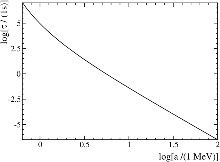
Figure 5: The proton mean proper lifetime $\tau$ associated with process (6) is plotted as a function of its proper acceleration $a$, where $m_{e}\lesssim a\lesssim m_{\pi}$.

Let us begin by rewriting the proper acceleration of the proton in Minkowski space, $a=R\Omega^{2}\gamma^{2}$ [see below Eq. (22)], in the form

$$a=\Omega\gamma\sqrt{\gamma^{2}-1}\;.$$ (3)

Now, we use General Relativity to obtain the proton’s energy per mass $E/m_{p}$ and angular velocity $d\phi/d\tau_{s}$ as calculated by a static observer lying at rest at the same radius of the particle orbit around a compact object with mass $M$. $E/m_{p}$ and $d\phi/d\tau_{s}$ are to be identified with $\gamma$ and $\Omega$ in Eq. (3), respectively, to obtain the proper acceleration $a$. Once we have $a$ and $\gamma$, we use Eqs. (52), (15), (40) and (7) to calculate the relevant decay rates and emitted powers. The results obtained in this way should be associated with the values defined by the static observers at the radius of the particle orbit. These ones differ from the reaction rates and emitted powers as measured at infinity by red-shift factors. In order to obtain (i) the reaction rates and (ii) the emitted powers at infinity from the ones measured by the static observers at the radius of the particle orbit, one should multiply the latter ones by (i) $\sqrt{1-2GM/r_{s}}$ and (ii) $1-2GM/r_{s}$, respectively. Although we can only capture with this procedure part of the influence of the spacetime curvature, its suitability as an approximate approach is justified by comparing the results which it provides with the ones obtained with full curved spacetime calculations, wherever the latter ones are available, as, e.g., in Ref. CHM .

The line element external to a spherically symmetric static object with mass $M$, which includes Schwarzschild black holes, can be written as

$$dS^{2}=\left(1-\frac{2GM}{r}\right)dt^{2}-\left(1-\frac{2GM}{r}\right)^{-1}dr^{2}-d\Sigma_{\Omega}^{2}\;,$$

where $d\Sigma_{\Omega}^{2}\equiv r^{2}(d\theta^{2}+(\sin\theta)^{2}d\phi^{2})$. According to General Relativity W , asymptotic observers associate an angular velocity $d\phi/dt_{a.o.}=\sqrt{GM/r_{s}^{3}}$ and an energy per mass ratio $E_{a.o.}/m=(1-2GM/r_{s})/\sqrt{1-3GM/r_{s}}$ for particles in circular geodesics at $r=r_{s}$. Thus, static observers at $r=r_{s}$ ($\theta,\phi={\rm const}$) associate the following corresponding values:

$$d\phi/d\tau_{s}={\sqrt{GM/r_{s}^{3}}}/\sqrt{1-2GM/r_{s}}$$

and

$$E/m_{p}=\sqrt{1-2GM/r_{s}}/\sqrt{1-3GM/r_{s}}\;.$$

By letting $d\phi/d\tau_{s}\to\Omega$ and $E/m_{p}\to\gamma$, we obtain

$$\gamma=\sqrt{\frac{1-2GM/r_{s}}{1-3GM/r_{s}}}$$ (4)

and [see Eq. (3)]

$$a=\frac{GM}{r_{s}^{2}(1-3GM/r_{s})}\;,$$ (5)

which will be used to evaluate Eqs. (52), (15), (40) and (7), whenever $\gamma\gg 1$. We note that Eqs. (4) and (5) are monotonic functions, which approximate the correct values asymptotically and diverge at $r_{s}=3GM$. This is so because according to General Relativity, circular geodesic orbits at $r_{s}\approx 3GM$ approximate lightlike worldlines.

At the last stable circular orbit, $r_{s}=6GM$, we obtain from Eq. (5) that

$$a/m_{e}=3\times 10^{-16}(M_{\odot}/M)\;.$$

Thus, protons around black holes in stable circular orbits $6GM<r_{s}<\infty$ are not likely to decay unless the compact object is a mini black hole with the mass of a mountain: $M\ll 10^{17}$ g [see Eq. (1)]. The fact that the smaller the black hole the more likely that protons decay at a fixed $r_{s}/(GM)$ is related with the fact that the smaller the black hole the larger the spacetime curvature, i.e. “gravitational field”, at the same $r_{s}/(GM)$.

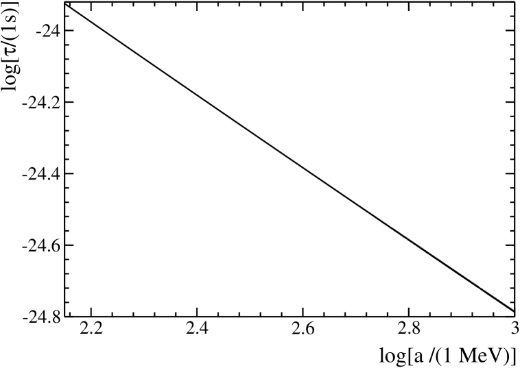
Figure 6: The proton mean proper lifetime $\tau$ associated with process (5) is plotted as a function of its proper acceleration $a$, where $m_{\pi}\lesssim a\lesssim m_{p}$.

In order to explore more realistic cases, where black holes have some solar masses, we have to consider protons at inner circular orbits, $3GM<r_{s}<6GM$, which are unstable. By defining $r_{s}\equiv 3GM(1+\delta)$ with $\delta\ll 1$ to monitor how far from the most internal circular orbit (at $r=3GM$) the proton is, we rewrite Eqs. (4) and (5) as

$$\gamma\approx 1/\sqrt{3\delta}$$ (6)

and

$$a\approx 1/(9GM\delta)\;.$$ (7)

By using Eqs. (6) and (7) in Eqs. (1) and (2) we obtain

$$3\times 10^{-19}(M_{\odot}/M)<\delta<9\times 10^{-17}(M_{\odot}/M)$$ (8)

and

$$5\times 10^{-20}(M_{\odot}/M)<\delta<3\times 10^{-19}(M_{\odot}/M)\;,$$ (9)

which are the intervals where the weak and strong processes would be favored, respectively. Thus, free protons in circular orbits around stellar mass black holes are likely to decay only if they are extremely close to the most internal circular geodesic and stay there for long enough to decay.

In Fig. 5, we plot from Eq. (52) the proton mean proper lifetime $\tau(a)=1/\Gamma_{f}^{p\to n}$ associated with the process (6), where $\Gamma_{f}^{p\to n}\equiv\gamma{\cal R}_{f}^{p\to n}$ is the weak transition probability per proper time and we have identified $G_{\rm eff}^{(f)}=G_{pn}$ with the Fermi coupling constant $G_{F}\equiv 1.166\times 10^{-5}\;{\rm GeV}^{-2}$. We have plotted the proper lifetime $\tau(a)$ rather than the laboratory lifetime $t(a)$ in order to make it easier the comparison of this figure with Fig. 1 in Ref. VM3 . In Fig. 6, we plot from Eq. (40) the proton mean proper lifetime $\tau(a)=1/\Gamma_{s}^{p\to n}$ associated with process (5), where $\Gamma_{s}^{p\to n}=\gamma{\cal R}_{s}^{p\to n}$ is the strong transition probability per proper time. Here $G_{\rm eff}^{(s)}$ is identified with the pion-nucleon-nucleon strong coupling constant $g_{\pi NN}$, which is written in the Heaviside-Lorentz system as $\sqrt{g_{\pi NN}^{2}/(4\pi)}\approx\sqrt{14}$ (see, e.g., GZ and MS ). Finally in Figs. 7 and 8, we plot the emitted power in the form of electrons and neutrinos as calculated from Eq. (15) and in the form of pions as calculated from (7), respectively.

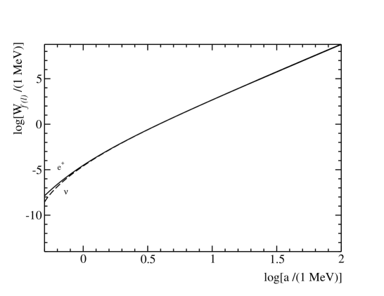
Figure 7: $W_{e^{+}}$ and $W_{\nu}$ associated with process (6) are plotted as functions of the proton proper acceleration $a$ with solid and dashed lines, respectively.

VI Discussion

The decay of accelerated protons has attracted interest for long time. Astrophysics seems to provide suitable conditions for the observation of the decay of accelerated protons. Cosmic ray protons with energy $E=\gamma m_{p}\approx 3\times 10^{14}$ eV under the influence of a magnetic field $H\approx 10^{14}$ Gauss of a pulsar have proper accelerations of $a_{H}=\gamma eH/m_{p}\approx 200$ MeV $>m_{\pi}$. For these values of $E$ and $H$, the proton are confined in a cylinder with typical radius $R\approx\gamma^{2}/a_{H}\approx 2\,\times\,10^{-2}\;{\rm cm}\ll l_{H}$, where $l_{H}$ is the typical size of the magnetic field region. Under such conditions, protons could rapidly decay through strong interaction before they lose most of their energy via electromagnetic synchrotron radiation TK .

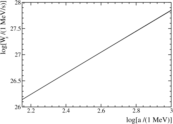
Figure 8: $W_{\pi}$ associated with process (5) is plotted as a function of the proton proper acceleration $a$.

Here we have considered the possible weak and strong proton decays under the influence of background gravitational fields. Reaction rates and emitted powers were calculated. We have concluded that they are unlikely to decay unless they orbit mini-black holes or they are pushed to highly relativistic geodesic circular orbits (and stay there for long enough to decay). This raises the question whether there would exist other astrophysical sites, where the decay rate could be larger. Perhaps the consideration of protons grazing the event horizon of black holes or entering properly the ergosphere of Kerr black holes extracting rotational energy from it would be worthwhile to be investigated. Notwithstanding because these cases would involve more complicated “trajectories” in a genuine general relativistic context, full quantum field theory in curved spacetime computations, rather than our semiclassical ones, would be desirable to provide more comprehensive results.

Acknowledgments

We are grateful to Gastão Krein for providing us with reference MS . D.F. and G.M. are thankful to Conselho Nacional de Desenvolvimento Científico e Tecnológico for full and partial supports, respectively. G.M. and D.V. acknowledge partial support from Fundação de Amparo à Pesquisa do Estado de São Paulo, while D.V. is also grateful to the US National Science Foundation for support under the Grant No PHY-0071044 in early stages of this project.

References

- (1) V. L. Ginzburg and G. F. Zharkov, Sov. Phys. JETP 20, 1525 (1965).
- (2) G. F. Zharkov, Sov. J. Nucl. Phys. 1, 120 (1965).
- (3) V. I. Ritus, Jour. Sov. Las. Research, 6, 497 (1985).
- (4) A. I. Nikishov and V. I. Ritus, Sov. Phys. JETP 19, 529 (1964); Sov. Phys. JETP 19, 1191 (1964).
- (5) V. I. Ritus, Sov. Phys. JETP 29, 532 (1969).
- (6) A. Tokuhisa and T. Kajino, Ap. J. 525, L117 (1999).
- (7) V. Berezinsky, A. Dolgov and M. Kachelriess, Phys. Lett. B 351, 261 (1995).
- (8) C. W. Misner, R. A. Breuer, D. R. Brill, P. L. Chrzanowski, H. G. Hughes III and C. M. Pereira, Phys. Rev. Lett. 28, 998 (1972). R. A. Breuer, P. L. Chrzanowski, H. G. Hughes III and C. W. Misner, Phys. Rev. D 8, 4309 (1973). R. A. Breuer, Gravitational Perturbation Theory and Synchrotron Radiation - Lecture Notes in Physics (Springer-Verlag, Heidelberg, 1975).
- (9) E. Poisson, Phys. Rev. D 52, 5719 (1995). L. M. Burko, Phys. Rev. Lett. 84, 4529 (2000). V. Cardoso and J. P. S. Lemos 65, 104033 (2002).
- (10) G. E. A. Matsas and D. A. T. Vanzella, Phys. Rev. D 59, 094004 (1999). D. A. T. Vanzella and G. E. A. Matsas, Phys. Rev. Lett. 87, 151301 (2001). H. Suzuki and K. Yamada, Phys. Rev. D 67, 065002 (2003).
- (11) S. A. Fulling, Phys. Rev. D 7, 2850 (1973); P. C. W. Davies, J. Phys. A 8, 609 (1975); W. G. Unruh, Phys. Rev. D 14, 870 (1976).
- (12) R. Muller, Phys. Rev. D 56, 953 (1997)
- (13) L. C. B. Crispino, A. Higuchi and G. E. A. Matsas, Class. Quantum Grav. 17, 19 (2000).
- (14) J. Castiñeiras, L. C. B. Crispino, R. Murta and G. E. A. Matsas, Phys. Rev. D 71, 104013 (2005).
- (15) D. A. T. Vanzella and G. E. A. Matsas, Phys. Rev. D 63, 014010 (2001).
- (16) C. Itzykson and J. -B. Zuber, Quantum Field Theory (McGraw-Hill, New York, 1980).
- (17) C. Quigg, Gauge Theory of the Strong, Weak, and Electromagnetic Interactions (Benjamin-Cummings, Reading, MA 1983).
- (18) I. S. Gradshteyn and I. M. Ryzhik, Table of Integrals, Series and Products (Academic, New York, 1980).
- (19) S. Takagi, Prog. Theor. Phys. Suppl. 88, 1 (1986).
- (20) Particle Data Group, C. Caso et al., Eur. Phys. J. C 3, 1 (1998).
- (21) V. N. Baier and V.M. Katkov, Sov. Phys. Dokl. 11, 947 (1967).
- (22) J. D. Landstreet, Phys. Rev. 153, 1372 (1967).
- (23) A. D. Kaminker, K. P. Levenfish and D. G. Yakovlev, Sov. Astron. Lett. 17, 450 (1991). A. D. Kaminker, K. P. Levenfish, D. G. Yakovlev, P. Amsterdamski, and P. Haensel, Phys. Rev. D 46, 3256 (1992).
- (24) A. Vidaurre, A. Pérez, H. Sivak, J. Bernabéu and J.Ma. Ibáñez, Astrop. J. 448, 264 (1995).
- (25) L. B. Leinson and A. Pérez, Phys. Rev. D 59, 043002 (1999).
- (26) V. B. Berestetskii, E. Lifshitz and L. P. Pitaevskii, Quantum Electrodynamics (Butterworth-Heinemann, Oxford, 1982). V. L. Ginzburg and S. I. Syrovatskii, Ann. Rev. Astron. Astrop. 3, 297 (1965).
- (27) V. N. Baier, V. M. Katkov, and V. M. Strakhovenko, Electromagnetic Processes at High Energies in Oriented Single Crystals (World Scientific, Singapore, 1998).
- (28) A. I. Nikishov, Journ. Sov. Laser Research 6, 619 (1985).
- (29) A. A. Gvozdev, A. V. Kuznetsov, N. V. Mikheev and L. A. Vassilevskaya, Proceed. IX Int. Baksan School “Particles and Cosmology (Ed.: E. N. Alexeev, V. A. Matveev, V. A. Rubakov and D. V. Semikoz, 1988), hep-ph 9709268.
- (30) R. M. Wald, General Relativity (University of Chicago Press, Chicago, 1984).
- (31) R. Machleidt and I. Slaus, J. Phys. G: Nucl. Part. Phys. 27, R69-R108 (2001)