Evolving wormhole geometries within nonlinear electrodynamics

Abstract

In this work, we explore the possibility of evolving $(2+1)$ and $(3+1)-$dimensional wormhole spacetimes, conformally related to the respective static geometries, within the context of nonlinear electrodynamics. For the $(3+1)-$dimensional spacetime, it is found that the Einstein field equation imposes a contracting wormhole solution and the obedience of the weak energy condition. Nevertheless, in the presence of an electric field, the latter presents a singularity at the throat, however, for a pure magnetic field the solution is regular. For the $(2+1)-$dimensional case, it is also found that the physical fields are singular at the throat. Thus, taking into account the principle of finiteness, which states that a satisfactory theory should avoid physical quantities becoming infinite, one may rule out evolving $(3+1)-$dimensional wormhole solutions, in the presence of an electric field, and the $(2+1)-$dimensional case coupled to nonlinear electrodynamics.

1 Introduction

Nonlinear electrodynamics has recently found many applications in several branches, namely, as effective theories at different levels of string/M-theory [1], cosmological models [2], black holes [3, 4], and in wormhole physics [4, 5, 6], amongst others. Pioneering work on nonlinear electrodynamic theories may be traced back to Born and Infeld [7], where the latter outlined a model to remedy the fact that the standard picture of a point charged particle possesses an infinite self-energy. Thus, the Born-Infeld model was founded on a principle of finiteness, that a satisfactory theory should avoid physical quantities becoming infinite. Furthermore, Plebański extended the examples of nonlinear electrodynamic Lagrangians [8], and demonstrated that the Born-Infeld theory satisfy physically acceptable requirements.

In this context, in a recent paper, it was shown that $(2+1)$ and $(3+1)-$dimensional static, spherically symmetric and stationary, axisymmetric traversable wormholes cannot be supported by nonlinear electrodynamics [6]. This is mainly due to the presence of an event horizon and that the null energy condition is not violated. However, a particularly interesting situation arouse in the analysis of the $(2+1)-$dimensional static and spherically symmetric wormholes, namely, that in order to construct these geometries, they must necessarily be supported by physical fields that become singular at the throat. Thus, taking into account the principle of finiteness, and imposing a non-singular behaviour of the physical quantities, it was found that the wormhole possesses an event horizon, rendering the geometry non-traversable. We also point out that the non-existence of $(3+1)-$dimensional static and spherically symmetric traversable wormholes is consistent with previous results [4].

Based on this analysis, it is also of interest to explore the specific case of evolving wormhole geometries, in the context of nonlinear electrodynamics. Time-dependent spherically symmetric wormholes have been extensively analysed in the literature, and a particularly interesting case of a dynamic wormhole immersed in an inflationary background, was considered by Roman [9]. The primary goal in the Roman analysis was to use inflation to enlarge an initially small, possibly submicroscopic, wormhole, and test whether one could evade the violation of the energy conditions in the process. Further dynamic wormhole geometries were analysed, considering specific cases [10, 11, 12], and the evolution of a wormhole model was considered in a FRW background [13]. In the latter model, it was found that the total stress-energy tensor does not necessarily violate the energy conditions as in the static Morris-Thorne case [14, 15]. Different scenarios for the weak energy condition violation were also explored, namely for a constant redshift function [10, 11], and an extension with a specific choice of a non-zero redshift function was further analysed [12].

Thus, in this work, we shall be interested in exploring the possibility that nonlinear electrodynamics may support time-dependent traversable wormhole geometries. This is of particular interest as the energy conditions are not necessarily violated in specific regions, as noted above. Therefore, analogously to Ref. [6], we shall consider $(2+1)$ and $(3+1)-$dimensional spacetimes and find particularly interesting results. We find that for the $(3+1)-$dimensional case in the presence of an electrical field, the latter becomes singular at the throat, however, for a purely magnetic field, the solution is regular at the throat, which is extremely promising, and is in close relationship to the regular magnetic black holes coupled to nonlinear electrodynamics found in Ref. [4]. For the $(2+1)-$dimensional case we find that the physical fields become singular at the throat.

This paper is outlined in the following manner: In section 2 we analyze $(3+1)-$dimensional dynamic and spherically symmetric wormholes coupled with nonlinear electrodynamics, and in section 3, $(2+1)-$dimensional evolving wormhole geometries in the context of nonlinear electrodynamics are studied. In section 4 we conclude. We shall use geometrised units, i.e., $G=c=1$, throughout this work .

2 $(3+1)-$dimensional wormhole

2.1 Action and spacetime metric

The action of $(3+1)-$dimensional general relativity coupled to nonlinear electrodynamics is given by

$$S=\int\sqrt{-g}\left[\frac{R}{16\pi}+L(F)\right]\,d^{4}x\,,$$ (1)

where $R$ is the Ricci scalar. $L(F)$ is a gauge-invariant electromagnetic Lagrangian, depending on a single invariant $F$ given by $F=F^{\mu\nu}F_{\mu\nu}/4$ [8], where $F_{\mu\nu}$ is the electromagnetic tensor. Note that in Einstein-Maxwell theory, the Lagrangian takes the form $L(F)=-F/4\pi$, however, we shall consider more general choices for the electromagnetic Lagrangians.

Varying the action with respect to the gravitational field provides the Einstein field equations $G_{\mu\nu}=8\pi T_{\mu\nu}$, with the stress-energy tensor given by

$$T_{\mu\nu}=g_{\mu\nu}\,L(F)-F_{\mu\alpha}F_{\nu}{}^{\alpha}\,L_{F}\,,$$ (2)

where $L_{F}=dL/dF$. The variation with respect to the electromagnetic potential $A_{\mu}$, where $F_{\mu\nu}=A_{\nu,\mu}-A_{\mu,\nu}$, yields the electromagnetic field equations

$$\left(F^{\mu\nu}\,L_{F}\right)_{;\mu}=0\,.$$ (3)

We shall consider that the spacetime metric representing a dynamic spherically symmetric $(3+1)-$dimensional wormhole, which is conformally related to the static wormhole geometry [14], takes the form

$$ds^{2}=\Omega^{2}(t)\left[-e^{2\Phi(r)}dt^{2}+\frac{dr^{2}}{1-b(r)/r}+r^{2}(d\theta^{2}+\sin^{2}{\theta}d\phi^{2})\right]\,,$$ (4)

where $\Phi$ and $b$ are functions of $r$, and $\Omega=\Omega(t)$ is the conformal factor, which is finite and positive definite throughout the domain of $t$. $\Phi$ is the redshift function, and $b(r)$ is denoted the form function [14]. We shall also assume that these functions satisfy all the conditions required for a wormhole solution, namely, $\Phi(r)$ is finite everywhere in order to avoid the presence of event horizons; $b(r)/r<1$, with $b(r_{0})=r_{0}$ at the throat; and the flaring out condition $(b-b^{\prime}r)/b^{2}\geq 0$, with $b^{\prime}(r_{0})<1$ at the throat.

Now, taking into account metric (4), the electromagnetic tensor, compatible with the symmetries of the geometry, is given by

$$F_{\mu\nu}=E(x^{\alpha})\;(\delta^{t}_{\mu}\delta^{r}_{\nu}-\delta^{r}_{\mu}\delta^{t}_{\nu})+B(x^{\alpha})\;(\delta^{\theta}_{\mu}\delta^{\phi}_{\nu}-\delta^{\phi}_{\mu}\delta^{\theta}_{\nu})\,,$$ (5)

where the non-zero components are the following: $F_{tr}=-F_{rt}=E$, the electric field, and $F_{\theta\phi}=-F_{\phi\theta}=B$, the magnetic field. The invariant $F$, included for self-completeness, takes the following form

$$F=-\frac{1}{2\Omega^{4}}\left[\left(1-\frac{b}{r}\right)e^{-2\Phi}\,E^{2}-\frac{B^{2}}{r^{4}\sin^{2}\theta}\right]\,.$$ (6)

2.2 Mathematics of embedding

To analyze evolving wormhole spacetimes, $\Phi(r)$ and $b(r)$ are chosen to provide a plausible wormhole geometry at $t=0$, which is assumed to be the onset of the evolution. One may verify the evolution of the wormhole considering the proper circumference $C_{0}$ of the throat, $r_{0}$, given by

$$C_{0}=\int_{0}^{2\pi}\Omega(t)\,r_{0}\,d\phi=\Omega(t)2\pi r_{0}\,,$$ (7)

and the radial proper length through the wormhole, between any two points $A$ and $B$ at any $t={\rm const}$, provided by

$$l(t)=\pm\Omega(t)\int_{r_{A}}^{r_{B}}\frac{dr}{(1-b/r)^{1/2}}=\Omega(t)\,l(t=0)\,,$$ (8)

which is simply the product of $\Omega(t)$ and the initial proper circumference and the radial proper separation, respectively.

One may use the mathematics of embedding to verify that the wormhole form of the metric is preserved with time. Here, we shall closely follow the analysis outlined in Ref. [9]. Due to the spherically symmetric nature of the problem, one may, without a significant loss of generality, consider an equatorial slice $\theta=\pi/2$. Considering, in addition, a fixed moment of time, $t={\rm const}$, the metric of the wormhole slice is given by

$$ds^{2}={\Omega^{2}(t)\,{dr^{2}}\over{1-b(r)/r}}+\Omega^{2}(t)\,r^{2}\,d\phi^{2}\,.$$ (9)

Now, to visualize this slice, this metric is embedded in a flat three dimensional Euclidean space with metric

$$ds^{2}=d{\bar{z}}^{2}+d{\bar{r}}^{2}+{\bar{r}}^{2}\,{d\phi}^{2}\,.$$ (10)

Comparing the respective coefficients of ${d\phi}^{2}$, one verifies the following relationships

$$\bar{r}={\Omega(t)\,r}\big{|}_{t={\rm const}}\,,\qquad{d\bar{r}}^{2}=\Omega^{2}(t)\,{dr}^{2}\big{|}_{t={\rm const}}\,.$$ (11)

However, it is important to emphasize, in particular, when considering derivatives, that equations (11) do not represent a coordinate transformation, but rather a rescaling of the $r$ coordinate on each $t={\rm constant}$ slice [9].

Note that the wormhole form of the metric will be preserved if the embedded metric, written in $\bar{z}$, $\bar{r}$ and $\phi$ coordinates, has the form

$$ds^{2}={{d{\bar{r}}^{2}}\over{1-{\bar{b}(\bar{r})/{\bar{r}}}}}+{\bar{r}}^{2}{d\phi}^{2}\,,$$ (12)

where $\bar{b}(\bar{r})$ has a minimum at some $\bar{b}(\bar{r}_{0})=\bar{r}_{0}$. Equation (9) can be rewritten in the form of equation (12) by using equations (11) and the definition $\bar{b}(\bar{r})=\Omega(t)\,b(r)$.

Using equations (10) and (12), one deduces $\bar{z}(\bar{r})=\Omega(t)\,z(r)$. Note that the relationship between the embedding space at an arbitrary time $t$ and the initial embedding space at $t=0$, using the above expressions, is given by

$$ds^{2}=d{\bar{z}}^{2}+d{\bar{r}}^{2}+{\bar{r}}^{2}\,{d\phi}^{2}=\Omega^{2}(t)\,[dz^{2}+dr^{2}+r^{2}{d\phi}^{2}]\,.$$ (13)

Relative to the $({\bar{z}},{\bar{r}},\phi)$ coordinate system the wormhole will always remain the same size, as the scaling of the embedding space compensates for the evolution of the wormhole. However, the wormhole will change size relative to the initial $t=0$ embedding space [9].

An important aspect of wormhole physics is the flaring out condition. From the above analysis, it follows that

$${{d\,^{2}{\bar{r}(\bar{z})}}\over{d{\bar{z}}^{2}}}=\frac{1}{\Omega(t)}\,{{b-b^{\prime}r}\over{2b^{2}}}=\frac{1}{\Omega(t)}\,{{d\,^{2}r(z)}\over{dz^{2}}}>0\,,$$ (14)

at or near the throat [14], so that the flaring out condition for the evolving wormhole is given by $d\,^{2}{\bar{r}(\bar{z})/d\bar{z}}^{2}>0$, in order to provide a wormhole solution. Taking into account equation (11), the definition of $\bar{b}(\bar{r})$, and $\bar{b}^{\prime}(\bar{r})=d\bar{b}/d\bar{r}=b^{\prime}(r)=db/dr$, one may rewrite equation (14) relative to the barred coordinates as $d\,^{2}{\bar{r}(\bar{z})}/d{\bar{z}}^{2}=\bar{b}-\bar{b}^{\prime}\bar{r}/(2{\bar{b}}^{2})>0$, at or near the throat. Thus, using barred coordinates, the flaring out condition has the same form as for the static wormhole [14].

2.3 Einstein field equations

For convenience, the non-zero Einstein tensor components, in an orthonormal reference frame, are given in A.1, and the stress-energy tensor components, using equation (2), in A.2. Now, using equation (70), i.e., $T_{\hat{t}\hat{r}}=0$, and the Einstein field equation, $G_{\hat{\mu}\hat{\nu}}=8\pi T_{\hat{\mu}\hat{\nu}}$, we verify from equation (65) that $\Phi^{\prime}=0$, considering the non-trivial case $\dot{\Omega}\neq 0$. Without a significant loss of generality, we choose $\Phi=0$, so that the nonzero components of the Einstein tensor, equations (63)-(66) reduce to

$$G_{\hat{t}\hat{t}} = \frac{1}{\Omega^{2}}\left[\frac{b^{\prime}}{r^{2}}+3\left(\frac{\dot{\Omega}}{\Omega}\right)^{2}\right]\,,$$ (15)

$$G_{\hat{r}\hat{r}} = \frac{1}{\Omega^{2}}\left\{-\frac{b}{r^{3}}+\left[\left(\frac{\dot{\Omega}}{\Omega}\right)^{2}-2\,\frac{\ddot{\Omega}}{\Omega}\right]\right\}\,,$$ (16)

$$G_{\hat{\theta}\hat{\theta}} = G_{\hat{\phi}\hat{\phi}}=\frac{1}{\Omega^{2}}\left\{-\frac{b^{\prime}r-b}{2r^{3}}+\left[\left(\frac{\dot{\Omega}}{\Omega}\right)^{2}-2\,\frac{\ddot{\Omega}}{\Omega}\right]\right\}\,,$$ (17)

where the overdot denotes a derivative with respect to the time coordinate, $t$, and the prime a derivative with respect to $r$. Note that the metric for this particular case is identical to the specific metric analyzed in Ref. [10].

Finally, taking into account that $\Phi=0$, the nonzero components of the stress energy tensor, from equations (67)-(69), take the following form

$$T_{\hat{t}\hat{t}} = -L-\frac{(1-b/r)}{\Omega^{4}}E^{2}L_{F}\,,$$ (18)

$$T_{\hat{r}\hat{r}} = L+\frac{(1-b/r)}{\Omega^{4}}E^{2}L_{F}\,,$$ (19)

$$T_{\hat{\theta}\hat{\theta}} = T_{\hat{\phi}\hat{\phi}}=L-\frac{1}{\Omega^{4}r^{4}\sin^{2}\theta}B^{2}L_{F}\,.$$ (20)

To impose the finiteness of the stress-energy tensor components, we shall also impose that $|(1-b/r)\,E^{2}\,L_{F}/\Omega^{4}|<\infty$ and $|B^{2}\,L_{F}/(\Omega^{4}r^{4}\sin^{2}\theta)|<\infty$, as $r\rightarrow r_{0}$.

An interesting feature immediately stands out, namely, that $T_{\hat{t}\hat{t}}=-T_{\hat{r}\hat{r}}$, so that using equations (15)-(16) through the Einstein field equation, we obtain the following relationship

$$\frac{b^{\prime}r-b}{2r^{3}}=-\left[2\left(\frac{\dot{\Omega}}{\Omega}\right)^{2}-\frac{\ddot{\Omega}}{\Omega}\right]\,.$$ (21)

Now, equation (21) can be solved separating variables and provides the following solutions,

$$b(r)=r\left[1-\alpha^{2}(r^{2}-r_{0}^{2})\right]\,,$$ (22)

$$\Omega(t)=\frac{2\alpha}{C_{1}\,e^{\alpha t}-C_{2}\,e^{-\alpha t}}\,,$$ (23)

where $\alpha$ is a constant, and $C_{1}$ and $C_{2}$ are constants of integration. Note that the form function reduces to $b(r_{0})=r_{0}$ at the throat, and $b^{\prime}(r_{0})=1-2\alpha^{2}r_{0}^{2}<1$ is also verified for $\alpha\neq 0$. Relatively to the conformal function, if $C_{1}=C_{2}$, then $\Omega$ is singular at $t=0$.

Thus, if $\alpha>0$, then we need to impose $C_{1}e^{\alpha t}>C_{2}e^{-\alpha t}$, and if $\alpha<0$ and $C_{1}e^{\alpha t}<C_{2}e^{-\alpha t}$, otherwise the conformal factor becomes singular somewhere along the domain of $t$. Now, $\Omega(t)\rightarrow 0$ as $t\rightarrow\infty$, which reflects a contracting wormhole solution. This analysis shows that one may, in principle, obtain an evolving wormhole solution in the range of the time coordinate. Note that $\alpha$ has the dimensions of (distance)^-1, so that it will be useful to define a dimensionless parameter $\beta=\alpha r_{0}$, so that the form function is given by

$$b(r)=r\left\{1-\beta^{2}\left[\left(\frac{r}{r_{0}}\right)^{2}-1\right]\right\}\,.$$ (24)

A fundamental condition to be a solution of a wormhole, is that $b(r)>0$ is imposed [16]. Thus, the range of $r$ is $r_{0}<r<a=r_{0}\sqrt{1+1/\beta^{2}}$, and the latter may be made arbitrarily large by taking $\beta\rightarrow 0$. If $a\gg r_{0}$, i.e., $\beta\simeq r_{0}/a\ll 1$, one may have an arbitrarily large wormhole. Note, however, that one may, in principle, match this solution to an exterior vacuum solution at a junction interface $R$, within the range $r_{0}<r<a$, much in the spirit of Refs. [16, 17].

It is also important to point out an interesting physical feature of this evolving, and in particular, contracting geometry, namely, the absence of the energy flux term, $T_{\hat{t}\hat{r}}=0$. One can interpret this aspect considering that the wormhole material is at rest in the rest frame of the wormhole geometry, i.e., an observer at rest in this frame is at constant $r,\,\theta,\,\phi$. The latter coordinate system coincides with the rest frame of the wormhole material, which can be defined as the one in which an observer co-moving with the material sees zero energy flux. This analysis is similar to the one outlined in Ref. [9].

In conclusion to this section, note that the solution outlined above possesses solely electromagnetic fields. One could also consider a non-interacting anisotropic time-dependent distribution of matter coupled to nonlinear electrodynamics. This may be reflected by the following superposition of the stress-energy tensor

$$T_{\mu\nu}=T_{\mu\nu}^{\rm fluid}+T_{\mu\nu}^{\rm NED}\,,$$ (25)

where $T_{\mu\nu}^{\rm NED}$ is given by Eq. (2), and $T_{\mu\nu}^{\rm fluid}$ is the anisotropic time-dependent stress-energy tensor associated with the fluid. A first approach reveals formidable calculations due to the time-dependence of the solution. Nevertheless, this is an interesting case to explore, and in particular the analysis of the energy conditions, which we leave for future work.

2.4 Energy conditions

We may further explore the energy conditions much in the spirit of Ref. [10], in particular, the weak energy condition (WEC), which is defined as $T_{\hat{\mu}\hat{\nu}}U^{\hat{\mu}}U^{\hat{\nu}}\geq 0$ where $U^{\hat{\mu}}$ is a timelike vector. The fact that the stress energy tensor is diagonal will be helpful, so that we need only to check the following three conditions

$$T_{\hat{t}\hat{t}}\geq 0\,,\qquad T_{\hat{t}\hat{t}}+T_{\hat{r}\hat{r}}\geq 0\,,\qquad T_{\hat{t}\hat{t}}+T_{\hat{\theta}\hat{\theta}}\geq 0\,,$$ (26)

which using equations (15)-(17), provide the following inequalities

$$\frac{1}{\Omega^{2}}\left[\frac{b^{\prime}}{r^{2}}+3\left(\frac{\dot{\Omega}}{\Omega}\right)^{2}\right]\geq 0\,,$$ (27)

$$\frac{1}{\Omega^{2}}\left\{\frac{b^{\prime}r-b}{2r^{3}}+\left[2\left(\frac{\dot{\Omega}}{\Omega}\right)^{2}-\frac{\ddot{\Omega}}{\Omega}\right]\right\}\geq 0\,,$$ (28)

$$\frac{1}{\Omega^{2}}\left\{\frac{b^{\prime}r+b}{2r^{3}}+2\left[2\left(\frac{\dot{\Omega}}{\Omega}\right)^{2}-\frac{\ddot{\Omega}}{\Omega}\right]\right\}\geq 0\,.$$ (29)

Note that inequality (28) reduces to the null energy condition (NEC) for a null vector oriented along the radial direction [10] (The NEC is defined as $T_{\hat{\mu}\hat{\nu}}k^{\hat{\mu}}k^{\hat{\nu}}\geq 0$ where $k^{\hat{\mu}}$ is a null vector). In fact, an interesting feature for the present $(3+1)-$dimensional evolving wormhole geometry coupled to nonlinear electrodynamics, is that the NEC is zero, for a null vector oriented along the radial direction. This may be inferred from equation (21), i.e., $T_{\hat{\mu}\hat{\nu}}k^{\hat{\mu}}k^{\hat{\nu}}=0$, for arbitrary $t$ and $r$. For inequality (29), using equations (21) and (24), we obtain $2r(1+\beta^{2})\geq 0$ which is always fulfilled. Finally, inequality (27), which is graphically depicted in figure 1, is also satisfied. We have defined $F(r,t)=[b^{\prime}/r^{2}+3(\dot{\Omega}/\Omega)^{2}]$, which represents the surface plotted in figure 1. The inequality (27) is represented as the region above the surface, and is manifestly positive.

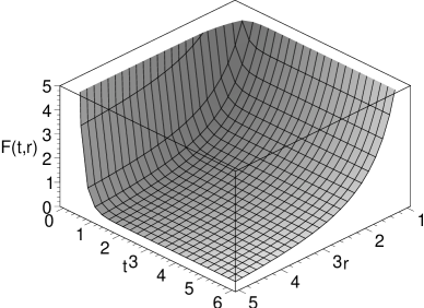
Figure 1: Plot of the inequality (27), which is given by the region above the surface. The latter is defined by $F(r,t)=[b^{\prime}/r^{2}+3(\dot{\Omega}/\Omega)^{2}]$, thus satisfying inequality (27). See the text for details.

We emphasize that for a static wormhole geometry the null energy condition, i.e., condition (28), is necessarily violated, consequently implying the violation of the WEC. However, this is not the case for dynamic wormhole spacetimes, as already pointed out in Ref. [10]. In the context of nonlinear electrodynamics, it was shown that $(3+1)-$dimensional static and spherically symmetric traversable wormholes cannot exist [4, 6], as the NEC is not violated, so that the flaring out condition is not verified. However, for the case of the evolving wormhole geometry analysed in this work, we have verified that the WEC is satisfied, as shown in the analysis above.

In the context of the energy conditions, a general class of higher dimensional wormhole geometries were constructed in an interesting paper [18], in which the four non-compact dimensions are static, and the possibility of time-dependent compact extra dimensions was explored. An interior wormhole solution was matched to an exterior vacuum solution, using the Synge junction conditions. The results of the analysis showed that: firstly, for the static case, where the gravitational field does not evolve in the full space, it is possible to respect the WEC at the throat, provided the extra dimensions place a restriction on the radial size of the wormhole throat; secondly, for the quasi-static case, where only the compact dimensions are time-dependent, the WEC cannot be satisfied at the throat. The latter result differs from the analysis within the context of non-linear electrodynamics explored in this work, where the time-dependent wormhole geometries satisfy the WEC. This is due to the fact that the higher dimensional solutions analysed in Ref. [18], the matter field does not possess an infinite spatial extent, due to the matter-vacuum junction boundary. As the models are now matched to the exterior vacuum, the time dependence of the extra dimensions is fixed by the vacuum and cannot de chosen arbitrarily, consequently resulting in the violation of the WEC (see Ref. [18] for further details).

2.5 Electromagnetic field equations

The electromagnetic field equation, equation (3), for calculational convenience, may be rewritten as

$$(F^{\mu\nu}L_{F})_{,\mu}=-F^{\mu\nu}\,\Gamma^{\alpha}_{\;\mu\alpha}\,L_{F}\,,$$ (30)

where $\Gamma^{\alpha}_{\;\mu\nu}$ are the Christoffel symbols of the second type. Setting $\nu=t$ and $\nu=r$, respectively, equation (30) can be solved, yielding the following solution for $EL_{F}$

$$EL_{F}=\frac{C_{E}}{r^{2}(1-b/r)^{1/2}}\,,$$ (31)

where $C_{E}$ is a constant or a function of $\theta$ only. From this last relation we verify that $EL_{F}$ is independent of the $t$ coordinate, and it is singular at the throat. Analogously, setting $\nu=\phi$, equation (30) can be solved, to provide the following relationship for $BL_{F}$

$$BL_{F}=C_{B}(t,r)\,\Omega^{4}\,r^{4}\,\sin\theta\,,$$ (32)

where $C_{B}$ is a constant of integration.

Another relationship, fundamental to our analysis, is the following

$$\left({}^{*}F^{\mu\nu}\right)_{;\mu}=0\,,$$ (33)

which can be deduced from the Bianchi identities, where ^∗ denotes the hodge dual [4]. Now, from equation (33), we obtain $\dot{B}=0$, $B^{\prime}=0$ and $E_{,\theta}=0$. Then, these conditions, together with equations (31) and (32) give us that $F_{tr}=-F_{tr}=E(t,r)$, $F_{\theta\phi}=-F_{\phi\theta}=B(\theta)$, $L_{F}=L_{F}(t,r)$. Thus, one may take $C_{E}=q_{\rm e}={\rm const}$, and note that the magnetic field is given by

$$B(\theta)=q_{\rm m}\,\sin\theta\,,$$ (34)

where $q_{\rm e}$ and $q_{\rm m}$ are constants related to the electric and magnetic charge, respectively.

Furthermore, from equations (15), (17), (18) and (20), we obtain

$$\frac{\Omega^{2}}{8\pi}\left(\frac{b^{\prime}r-3b}{2r^{3}}\right)=\left(1-\frac{b}{r}\right)\,E^{2}\,L_{F}+\frac{q_{\rm m}^{2}}{r^{4}}L_{F}\,.$$ (35)

Considering a non-zero electric field, $E\neq 0$, we can use equations (31) and (35) to obtain

$$E(t,r)=\frac{(b^{\prime}r-3b)\Omega^{2}r\pm\sqrt{(b^{\prime}r-3b)^{2}\Omega^{4}r^{2}-(32\pi q_{\rm e}q_{\rm m})^{2}}}{32\pi q_{\rm e}r^{2}(1-b/r)^{1/2}}\,.$$ (36)

From this solution we point out two observations: (i) we require that $(b^{\prime}r-3b)^{2}\Omega^{2}r^{2}>(32\pi q_{\rm e}q_{\rm m})^{2}$ so we have a limiting (interval) inequality; (ii) and that $E$ is inversely proportional to $(1-b/r)^{-1/2}$, showing that the $E$ field is singular at the throat, which is in contrast to the principle of finiteness. Finally, and for completeness, we have

$$L_{F}=\frac{32q_{\rm e}^{2}\pi}{(b^{\prime}r-3b)\Omega^{2}r\pm\sqrt{(b^{\prime}r-3b)^{2}\Omega^{4}r^{2}-(32\pi q_{\rm e}q_{\rm m})^{2}}}\,.$$ (37)

2.5.1 $B=0$.

In particular, consider the case of $B=0$, so that using equations (15)-(16), (18)-(19) and (21), we find

$$E^{2}L_{F}=\frac{\Omega^{2}}{16\pi}\frac{b^{\prime}r-3b}{r^{3}(1-b/r)}\,,$$ (38)

which together with equation (31) provides

$$E=\frac{\Omega^{2}}{16\pi q_{\rm e}}\frac{b^{\prime}r-3b}{r(1-b/r)^{1/2}}\,,$$ (39)

and

$$L_{F}=\frac{16\pi q_{\rm e}^{2}}{\Omega^{2}r(b^{\prime}r-3b)}\,.$$ (40)

Note that even if $B=0$ the expression for $E$ is singular at the throat.

In the analysis outlined above, namely, in the presence of an electric field, we verify a problematic issue, namely, that the latter presents a singularity at the throat. This is an extremely troublesome aspect of the geometry, and we emphasize that this is in contradiction to the model construction of nonlinear electrodynamics, founded on a principle of finiteness, that a satisfactory theory should avoid physical quantities becoming infinite [7]. Thus, one should impose that these physical quantities be non-singular, and in doing so, we may rule out $(3+1)-$dimensional dynamical spherically symmetric wormhole solutions, in the presence of electric fields, within the context of nonlinear electrodynamics.

2.5.2 $E=0$.

An interesting case arises setting $E=0$. Using equation (35), we obtain

$$L_{F}=\frac{1}{16\pi q_{\rm m}^{2}}\Omega^{2}r(b^{\prime}r-3b)\,,$$ (41)

and taking into account equations (15) and (18), the Lagrangian is given by

$$L=-\frac{1}{8\pi\Omega^{2}}\left[\frac{b^{\prime}}{r^{2}}+3\left(\frac{\dot{\Omega}}{\Omega}\right)^{2}\right]\,.$$ (42)

These equations, together with $B=q_{\rm m}\sin\theta$, $E=0$, $F=q_{\rm m}^{2}/(2\Omega^{4}r^{4})$ and solutions (22) and (23) give a wormhole solution without problems at the throat, with finite fields. This result is in close relationship to the regular magnetic black holes coupled to nonlinear electrodynamic found in Ref. [4].

3 $(2+1)-$dimensional wormhole

3.1 Action and spacetime metric

We shall also be interested in $(2+1)-$dimensional general relativity coupled to nonlinear electrodynamics. The respective action is given by

$$S=\int\sqrt{-g}\left[\frac{R}{16\pi}+L(F)\right]\,d^{3}x\,,$$ (43)

where $L(F)$ is a gauge-invariant electromagnetic Lagrangian, which we shall leave unspecified at this stage, depending on a single invariant $F$ given by $F=F^{\mu\nu}F_{\mu\nu}/4$. The factor $1/16\pi$ is maintained in the action to keep the parallelism with $(3+1)-$dimensional theory. The Maxwell Lagrangian is recovered in the weak field limit, i.e., $L(F)\rightarrow-F/4\pi$. Analogously to the $(3+1)-$dimensional case, by varying the action with respect to the gravitational field, one obtains the Einstein field equations $G_{\mu\nu}=8\pi T_{\mu\nu}$, where the stress-energy tensor is given by

$$T_{\mu\nu}=g_{\mu\nu}\,L(F)-F_{\mu\alpha}F_{\nu}{}^{\alpha}\,L_{F}\,.$$ (44)

Varying the action with respect to the electromagnetic potential, one obtains the electromagnetic field equation, $(F^{\mu\nu}\,L_{F})_{;\mu}=0$.

Consider the time-dependent spherically symmetric $(2+1)-$dimensional wormhole spacetime, and which is given by the following metric

$$ds^{2}=\Omega^{2}(t)\left[-e^{2\Phi}dt^{2}+\frac{dr^{2}}{1-b/r}+r^{2}d\phi^{2}\right]\,.$$ (45)

Taking into account the symmetries of the geometry, we shall consider the following electromagnetic tensor

$$F_{\mu\nu}=E(x^{\alpha})(\delta^{t}_{\mu}\delta^{r}_{\nu}-\delta^{r}_{\mu}\delta^{t}_{\nu})+B(x^{\alpha})(\delta^{\phi}_{\mu}\delta^{r}_{\nu}-\delta^{r}_{\mu}\delta^{\phi}_{\nu})\,,$$ (46)

where the nonzero components are given by $F_{tr}=-F_{rt}=E(x^{\alpha})$ and $F_{\phi r}=-F_{r\phi}=B(x^{\alpha})$. We shall include the expression for the invariant $F$, for self-completeness, which is given by

$$F=-\frac{1}{2}\,\frac{(1-b/r)}{\Omega^{2}}\,\left(e^{-2\Phi}\,E^{2}-\frac{1}{r^{2}}B^{2}\right)\,.$$ (47)

3.2 Field equations

The non-zero Einstein tensor components are given in B.1, and the respective stress-energy tensor components in B.2. Analogously for the $(3+1)-$dimensional case, note that $T_{\hat{t}\hat{r}}=0$, and using the Einstein field equation, $G_{\hat{\mu}\hat{\nu}}=8\pi T_{\hat{\mu}\hat{\nu}}$, we verify from equation (74) that $\Phi^{\prime}=0$, considering the non-trivial case $\dot{\Omega}\neq 0$. Once again, one may consider $\Phi=0$, without a loss of generality, so that the nonzero components of the Einstein tensor, equations (71)-(73), may be rewritten as

$$G_{\hat{t}\hat{t}} = \frac{1}{\Omega^{2}}\left[\frac{b^{\prime}r-b}{2r^{3}}+\left(\frac{\dot{\Omega}}{\Omega}\right)^{2}\right]\,,$$ (48)

$$G_{\hat{r}\hat{r}} = G_{\hat{\phi}\hat{\phi}}=\frac{1}{\Omega^{2}}\left[\left(\frac{\dot{\Omega}}{\Omega}\right)^{2}-\frac{\ddot{\Omega}}{\Omega}\right]\,,$$ (49)

and the respective nonzero components of the stress energy tensor, equations (75)-(77), take the form

$$T_{\hat{t}\hat{t}}=-L-\frac{(1-b/r)}{\Omega^{4}}E^{2}L_{F}\,,$$ (50)

$$T_{\hat{r}\hat{r}}=L+\frac{(1-b/r)}{\Omega^{4}}E^{2}L_{F}-\frac{(1-b/r)}{r^{2}\Omega^{4}}B^{2}L_{F}\,,$$ (51)

$$T_{\hat{\phi}\hat{\phi}}=L-\frac{(1-b/r)}{r^{2}\Omega^{4}}B^{2}L_{F}\,.$$ (52)

Furthermore, from equations (49) and (51)-(52), using the Einstein field equation we verify that $E=0$, ignoring the trivial case $L_{F}=0$. Note that from $T_{\hat{t}\hat{\phi}}$, equation (79) one has $E\cdot B=0$, which is consistent with $E=0$, as found above. Thus, the stress energy components reduce to

$$T_{\hat{t}\hat{t}} = -L\,,$$ (53)

$$T_{\hat{r}\hat{r}} = T_{\hat{\phi}\hat{\phi}}=L-\frac{(1-b/r)}{r^{2}\Omega^{4}}B^{2}L_{F}\,,$$ (54)

and the Lagrangian is given by

$$L=-\frac{1}{8\pi\Omega^{2}}\left[\frac{b^{\prime}r-b}{2r^{3}}+\left(\frac{\dot{\Omega}}{\Omega}\right)^{2}\right]\,.$$ (55)

We can now calculate the WEC, by taking into account equations (48)-(49), to obtain the following relationships

$$\frac{1}{\Omega^{2}}\left[\frac{b^{\prime}r-b}{2r^{3}}+\left(\frac{\dot{\Omega}}{\Omega}\right)^{2}\right]\geq 0\,,$$ (56)

$$\frac{1}{\Omega^{2}}\left\{\frac{b^{\prime}r-b}{2r^{3}}+\left[2\left(\frac{\dot{\Omega}}{\Omega}\right)^{2}-\frac{\ddot{\Omega}}{\Omega}\right]\right\}\geq 0\,.$$ (57)

From the electromagnetic field equations, we obtain $F^{\mu t}{}_{;\mu}=0$ and $F^{\mu r}{}_{;\mu}=0$ and

$$\frac{(1-b/r)}{r^{2}\Omega^{4}}\,B\,\left[\log(L_{F})\right]_{,r}=F^{\mu\phi}{}_{;\mu}\,.$$ (58)

Equation (58) can be solved to provide

$$BL_{F}=\frac{C_{t}r}{(1-b/r)^{1/2}}\,,$$ (59)

where $C_{t}$ is a constant or a function of $t$ only. Furthermore, from equations (53)-(54) we obtain

$$B^{2}L_{F}=-\frac{\Omega^{2}r^{2}}{8\pi(1-b/r)}\left\{\frac{b^{\prime}r-b}{2r^{3}}+\left[2\left(\frac{\dot{\Omega}}{\Omega}\right)^{2}-\frac{\ddot{\Omega}}{\Omega}\right]\right\}\,.$$ (60)

Thus, using equations (59) and (60), we find

$$B(t,r)=-\frac{1}{8\pi C_{t}}\frac{\Omega^{2}r}{(1-b/r)^{1/2}}\left\{\frac{b^{\prime}r-b}{2r^{3}}+\left[2\left(\frac{\dot{\Omega}}{\Omega}\right)^{2}-\frac{\ddot{\Omega}}{\Omega}\right]\right\}\,,$$ (61)

and

$$L_{F}(t,r)=-\frac{8\pi C_{t}^{2}}{\Omega^{2}}\left\{\frac{b^{\prime}r-b}{2r^{3}}+\left[2\left(\frac{\dot{\Omega}}{\Omega}\right)^{2}-\frac{\ddot{\Omega}}{\Omega}\right]\right\}^{-1}\,.$$ (62)

From equation (61), one verifies that the field $B$ is singular at the throat. Analogously to the $(3+1)-$ dimensional case, this is an extremely troublesome aspect of the geometry, as in order to construct a traversable wormhole, singularities appear in the physical fields, which is in contradiction to the model construction of nonlinear electrodynamics, founded on a principle of finiteness [7]. Thus, one should impose that these physical quantities be non-singular, and in doing so, we verify that we cannot afford a wormhole type solution.

4 Conclusion

In a recent paper, it was shown that $(2+1)$ and $(3+1)-$dimensional static, spherically symmetric and stationary, axisymmetric traversable wormholes cannot be supported by nonlinear electrodynamics. In this work, we explored the possibility of evolving time-dependent wormhole geometries coupled to nonlinear electrodynamics. For the $(3+1)-$dimensional spacetimes, it was found that the Einstein field equation imposes a contracting wormhole solution and that the weak energy condition be satisfied. It was also found that in the presence of an electric field, a problematic issue was verified, namely, that the latter become singular at the throat. However, regular solutions of traversable wormholes in the presence of a pure magnetic field were found. Time-dependent spherically symmetric $(2+1)-$dimensional wormhole spacetimes were also analyzed, and it was found that the Einstein field equation imposes that the electric field be zero. For this case, it was found that in order to construct wormhole geometries, these must necessarily be supported by physical fields that become singular at the throat. Thus, taking into account that the model construction of nonlinear electrodynamics, founded on the principle of finiteness, that a satisfactory theory should avoid physical quantities becoming infinite, one may rule out evolving $(3+1)-$dimensional electric wormhole solutions, and the $(2+1)-$dimensional case coupled to nonlinear electrodynamics.

It is also relevant to emphasize that the solutions obtained in this work and in Ref. [6], can be obtained using an alternative form of nonlinear electrodynamics, denoted the $P$ framework [4]. The latter is obtained from the original form, the $F$ framework, by a Legendre transformation. The duality between the $F$ and $P$ frameworks connects solutions of different theories, but we emphasize that it is a dual description of the same physical system. Therefore, we have not made use of the $P$ formalism throughout this work, as we have only been interested in exploring the possible existence of evolving wormhole solutions coupled to nonlinear electrodynamics. Another point worth noting is that we have only considered that the gauge-invariant electromagnetic Lagrangian $L(F)$ be dependent on a single invariant $F$. As stressed in Ref. [6], it would also be worthwhile to include another electromagnetic field invariant $G\sim\,^{*}F^{\mu\nu}\,F_{\mu\nu}$, which would possibly add an interesting analysis to the solutions found in this work.

Appendix A $(3+1)-$dimensional evolving wormhole geometry

A.1 Einstein tensor

The non-zero components of the Einstein tensor, given in an orthonormal reference frame, for the metric (4), are the following

$$G_{\hat{t}\hat{t}}=\frac{1}{\Omega^{2}}\,\left[3e^{-2\Phi}\,\left(\frac{\dot{\Omega}}{\Omega}\right)^{2}+\frac{b^{\prime}}{r^{2}}\right]\,,$$ (63)

$$G_{\hat{r}\hat{r}}=\frac{1}{\Omega^{2}}\;\left\{e^{-2\Phi(r)}\,\left[{\left({{\dot{\Omega}}\over{\Omega}}\right)^{2}}-2\,\frac{\ddot{\Omega}}{\Omega}\right]-\left[{b\over{r^{3}}}-2\,\frac{\Phi^{\prime}}{r}\,\left(1-\frac{b}{r}\right)\right]\right\}\,,$$ (64)

$$G_{\hat{t}\hat{r}}=2\,\frac{\dot{\Omega}}{\Omega^{3}}\;e^{-\Phi}\,\Phi^{\prime}\left(1-\frac{b}{r}\right)^{1/2}\,,$$ (65)

$$G_{\hat{\theta}\hat{\theta}}=G_{\hat{\phi}\hat{\phi}}=\frac{1}{\Omega^{2}}\;\Bigg{\{}e^{-2\Phi(r)}\,\left[\left(\frac{\dot{\Omega}}{\Omega}\right)^{2}-2\,\frac{\ddot{\Omega}}{\Omega}\right]+\left(1-\frac{b}{r}\right)\times$$

$$\times\left[\Phi^{\prime\prime}+(\Phi^{\prime})^{2}-\frac{b^{\prime}r-b}{2r(r-b)}\Phi^{\prime}-\frac{b^{\prime}r-b}{2r^{2}(r-b)}+\frac{\Phi^{\prime}}{r}\right]\Bigg{\}}\,,$$ (66)

where the overdot denotes a derivative with respect to the time coordinate, $t$, and the prime a derivative with respect to $r$.

A.2 Stress-energy tensor

The components of the stress energy tensor, equation (2), in the orthonormal frame, take the following form

$$T_{\hat{t}\hat{t}} = -L-\frac{e^{-2\Phi}(1-b/r)}{\Omega^{4}}E^{2}L_{F}\,,$$ (67)

$$T_{\hat{r}\hat{r}} = L+\frac{e^{-2\Phi}(1-b/r)}{\Omega^{4}}E^{2}L_{F}\,,$$ (68)

$$T_{\hat{\theta}\hat{\theta}} = T_{\hat{\phi}\hat{\phi}}=L-\frac{1}{\Omega^{4}r^{4}\sin^{2}\theta}B^{2}L_{F}\,,$$ (69)

$$T_{\hat{t}\hat{i}} = T_{\hat{i}\hat{j}}=0\quad({\rm with}\;\;i\neq j)\,.$$ (70)

Appendix B $(2+1)-$dimensional evolving wormhole geometry

B.1 Einstein tensor

Using the orthonormal reference frame we have that the nonzero components of the Einstein tensor, for the metric (45), are

$$G_{\hat{t}\hat{t}} = \frac{1}{\Omega^{2}}\left[\frac{b^{\prime}r-b}{2r^{3}}+e^{-2\Phi}\left(\frac{\dot{\Omega}}{\Omega}\right)^{2}\right]\,,$$ (71)

$$G_{\hat{r}\hat{r}} = \frac{1}{\Omega^{2}}\left\{\left(1-\frac{b}{r}\right)\frac{\Phi^{\prime}}{r}+e^{-2\Phi}\left[\left(\frac{\dot{\Omega}}{\Omega}\right)^{2}-\frac{\ddot{\Omega}}{\Omega}\right]\right\}\,,$$ (72)

$$G_{\hat{\phi}\hat{\phi}} = \frac{1}{\Omega^{2}}\Bigg{\{}\left(1-\frac{b}{r}\right)\left[\Phi^{\prime\prime}+(\Phi^{\prime})^{2}-\frac{b^{\prime}r-b}{2r(r-b)}\Phi^{\prime}\right]+e^{-2\Phi}\left[\left(\frac{\dot{\Omega}}{\Omega}\right)^{2}-\frac{\ddot{\Omega}}{\Omega}\right]\Bigg{\}}\,,$$ (73)

$$G_{\hat{t}\hat{r}} = \frac{1}{\Omega^{2}}\left[\left(1-\frac{b}{r}\right)^{1/2}\Phi^{\prime}\;e^{-\Phi}\left(\frac{\dot{\Omega}}{\Omega}\right)\right]\,.$$ (74)

B.2 Stress-energy tensor

The components of the stress energy tensor, equation (44), in the orthonormal frame, take the following form

$$T_{\hat{t}\hat{t}} = -L-\frac{e^{-2\Phi}(1-b/r)}{\Omega^{4}}E^{2}L_{F}\,,$$ (75)

$$T_{\hat{r}\hat{r}} = L+\frac{e^{-2\Phi}(1-b/r)}{\Omega^{4}}E^{2}L_{F}-\frac{(1-b/r)}{r^{2}\Omega^{4}}B^{2}L_{F}\,,$$ (76)

$$T_{\hat{\phi}\hat{\phi}} = L-\frac{(1-b/r)}{r^{2}\Omega^{4}}B^{2}L_{F}\,,$$ (77)

$$T_{\hat{t}\hat{r}} = 0\,,$$ (78)

$$T_{\hat{t}\hat{\phi}} = -\frac{e^{-\Phi}(1-b/r)}{\Omega^{2}r}\,\,E\,B\,L_{F}\,,$$ (79)

$$T_{\hat{r}\hat{\phi}} = 0\,.$$ (80)

References

References

- [1] N. Seiberg and E. Witten, “String theory and noncommutative geometry,” JHEP 9909, 032 (1999) [arXiv:hep-th/9908142].
- [2] M. Novello, S. E. P. Bergliaffa and J. Salim, “Nonlinear electrodynamics and the acceleration of the universe,” Phys. Rev. D 69 127301 (2004) [arXiv:astro-ph/0312093]. P. V. Moniz, “Quintessence and Born-Infeld cosmology,” Phys. Rev. D 66, 103501 (2002). R. Garcia-Salcedo and N. Breton, “Born-Infeld Cosmologies,” Int. J. Mod. Phys. A15, 4341-4354 (2000) [arXiv:gr-qc/0004017]. R. Garcia-Salcedo and N. Breton, “Nonlinear electrodynamics in Bianchi spacetimes,” Class. Quant. Grav. 20, 5425-5437 (2003) [arXiv:hep-th/0212130]. R. Garcia-Salcedo and N. Breton, “Singularity-free Bianchi spaces with nonlinear electrodynamics,” Class. Quant. Grav. 22, 4783-4802 (2005) [arXiv:gr-qc/0410142]. V. V. Dyadichev, D. V. Gal’tsov, A. G. Zorin and M. Yu. Zotov, “Non-Abelian Born–Infeld cosmology,” Phys. Rev. D 65, 084007 (2002) [arXiv:hep-th/0111099]. D. N. Vollick, “Anisotropic Born-Infeld Cosmologies,” Gen. Rel. Grav. 35, 1511-1516 (2003) [arXiv:hep-th/0102187].
- [3] E. Ayón-Beato and A. García, “Regular black hole in general relativity coupled to nonlinear electrodynamics,” Phys. Rev. Lett. 80, 5056-5059 (1998) [arXiv:gr-gc/9911046]. E. Ayón-Beato and A. García, “New regular black hole solution from non-linear electrodynamics,” Phys. Lett. B 464, 25 (1999) [arXiv:hep-th/9911174]; E. Ayón-Beato and A. García, “Non-singular charged black hole solutions for non-linear source,” Gen. Rel. Grav. 31, 629-633 (1999) [arXiv:gr-gc/9911084]. M. Cataldo and A. García, “Regular dimensional black holes within non-linear electrodynamics,” Phys. Rev. D 61, 084003 (2000) [arXiv:hep-th/0004177]. A. Burinskii and S. R. Hildebrandt, “New type of regular black holes and particlelike solutions from nonlinear electrodynamics,” Phys. Rev. D 65, 104017 (2002) [arXiv:hep-th/0202066]. N. Breton, “Stability of nonlinear magnetic black holes,” Phys. Rev. D 72, 044015 (2005) [arXiv:hep-th/0502217].
- [4] K. A. Bronnikov, “Regular magnetic black holes and monopoles from nonlinear electrodynamics,” Phys. Rev. D 63, 044005 (2001) [arXiv:gr-qc/0006014].
- [5] F. Baldovin, M. Novello, S. E. Perez Bergliaffa and J.M. Salim , “A nongravitational wormhole,” Class. Quant. Grav. 17, 3265-3276 (2000) [arXiv:gr-qc/0003075]. K. A. Bronnikov and S. V. Grinyok, “Electrically charged and neutral wormhole instability in scalar-tensor gravity,” Grav. Cosmol. 11, 75-81 (2006) [arXiv:gr-qc/0509062].
- [6] A. V. B. Arellano and F. S. N. Lobo, “Traversable wormholes coupled to nonlinear electrodynamics,” [arXiv:gr-qc/0604095].
- [7] M. Born, “On the quantum theory of the electromagnetic field,” Proc. Roy. Soc. Lond. A143, 410 (1934); A144, 425 (1934); M. Born and L. Infeld, Proc. Roy. Soc. Lond. A147, 522 (1934).
- [8] J. F. Plebański, “Lectures on non-linear electrodynamics,” monograph of the Niels Bohr Institute Nordita, Copenhagen (1968). S. A. Gutiérrez, A. L. Dudley and J. F. Plebański, “Signals and discontinuities in general relativistic nonlinear electrodynamics,” J. Math. Phys. 22, 2835 (1981).
- [9] T. A. Roman, “Inflating Lorentzian wormholes,” Phys. Rev. D 47, 1370 (1993) [arXiv:gr-qc/9211012].
- [10] S. Kar, “Evolving wormholes and the energy conditions,” Phys. Rev. D 49, 862 (1994).
- [11] S. Kar and D. Sahdev, “Evolving Lorentzian wormholes,” Phys. Rev. D 53, 722 (1996) [arXiv:gr-qc/9506094].
- [12] L. A. Anchordoqui, D. F. Torres and M. L. Trobo, “Evolving wormhole geometries,” Phys. Rev. D 57, 829 (1998) [arXiv:gr-qc/9710026].
- [13] S. W. Kim, “Cosmological model with a traversable wormhole,” Phys. Rev. D 53, 6889 (1996).
- [14] M. Morris and K.S. Thorne, “Wormholes in spacetime and their use for interstellar travel: A tool for teaching General Relativity,” Am. J. Phys. 56, 395 (1988).
- [15] Visser M 1995 Lorentzian Wormholes: From Einstein to Hawking (American Institute of Physics, New York).
- [16] J. P. S. Lemos, F. S. N. Lobo and S. Q. de Oliveira, “Morris-Thorne wormholes with a cosmological constant,” Phys. Rev. D 68, 064004 (2003) [arXiv:gr-qc/0302049].
- [17] J. P. S. Lemos and F. S. N. Lobo, “Plane symmetric traversable wormholes in an anti-de Sitter background,” Phys. Rev. D 69, 104007 (2004) [arXiv:gr-qc/0402099]; F. S. N. Lobo, “Surface stresses on a thin shell surrounding a traversable wormhole,” Class. Quant. Grav. 21, 4811 (2004) [arXiv:gr-qc/0409018]; F. S. N. Lobo, “Energy conditions, traversable wormholes and dust shells,” Gen. Rel. Grav. 37 2023-2038 (2005) [arXiv:gr-qc/0410087]; F. S. N. Lobo and P. Crawford, “Stability analysis of dynamic thin shells,” Class. Quant. Grav. 22, 4869 (2005), [arXiv:gr-qc/0507063]; F. S. N. Lobo, “Phantom energy traversable wormholes,” Phys. Rev. D 71, 084011 (2005) [arXiv:gr-qc/0502099]; F. S. N. Lobo, “Stability of phantom wormholes,” Phys. Rev. D 71, 124022 (2005) [arXiv:gr-qc/0506001]; F. S. N. Lobo, “Stable dark energy stars,” Class. Quant. Grav. 23, 1525 (2006) [arXiv:astro-ph/0508115].
- [18] A. DeBenedictis and A. Das, “Higher dimensional wormhole geometries with compact dimensions,” Nucl. Phys. B 653, 279-304 (2003) [arXiv:gr-qc/0207077].