A New Action-Derived Form of The Black Hole Metric

Abstract:

Several different but equivalent forms of the spherical black hole (Schwarzschild) are known, as well as several derivations. Here a novel form is derived through the power of the action formalism. The method generalizes to any spherical black hole or brane, and the charged hole case (Reissner-Nordström) is worked out in detail.

To Eitan Aharoni,                        
my friend ever since the 7th grade,
who always encourages me             
to examine fundamental issues.

Introduction. In 1916 Schwarzschild [1] discovered the metric which bears his name, and in perspective it is recognized as the first black hole. It is static, spherically symmetric and uncharged.

By now several equivalent analytical metrics are known, all describing the same black hole, while each one highlights different properties. Each such metric is usually derived by choosing a gauge for the metric, writing the Einstein equations and then solving them. In general, while a given result may be proven in many ways, some scientists believe that “somewhere” there exists a “book” with “the proof”. In this paper we shall describe such a unique derivation for the metric of spherical black holes.

Very generally in physics it is known that an action, when available, is the most concise packaging of the equations of motion, and moreover it enables the widest class of field transformations. Still in General Relativity (GR) traditionally one writes down the equations of motion, even though an action principle is known. The reason for that is the large gauge symmetry: in order for the action to encode all the equations, it must be written as a function of as many fields as there are equations, while in GR, and in particular in deriving black hole metrics, it is common practice to start by fixing the gauge (an ansatz for the metric) in order to minimize the number of fields involved and to simplify the equations.

Owing to its advantages, this paper takes the action approach to derive the black hole metric. In order not to lose any of the Einstein equations it is essential to keep a larger set of metric components than in a “most general” ansatz, but not all of them (in the presence of isometries), as discussed below in detail. This has the benefit that the gauge can be chosen rationally rather than arbitrarily, according to the form of the action. As we shall see below, the gauge can be chosen according to the standard requirement that the kinetic term be canonical. This in turn will simplify the equations of motion and will lead to a new form of the black hole metric.

Ansatz. Consider a spherical black hole in General Relativity (so that the only field is the space-time metric) in asymptotically flat $d$-dimensional space-time, namely the Schwarzschild black hole [1] (see [4] for a generalization to $d\neq 4$).

Which fields must be kept in an action approach? For a generic metric we need to keep all the metric components $g_{\mu\nu}$ in order to encode all the equations, namely all the components of the Einstein tensor $G_{\mu\nu}$. However, in the common case of a metric with isometries a reduction in the number of fields is possible. Given a metric which preserves the isometries, its Einstein tensor is invariant as well, and in particular some of its components necessarily vanish. Correspondingly fewer fields are required.

For the case at hand, the spherical black hole, with its $SO(d-1)_{\Omega}\times U(1)_{t}\times\hbox{Z\kern-3.99994ptZ}_{2,t}$ isometries, namely spherical, stationary and time reflection, respectively, this “maximally general ansatz” is given by

$$ds^{2}=-e^{2\,A}\,dt^{2}+e^{2\,B}\,dx^{2}+e^{2\,C}\,d\Omega^{2}_{d-2}~{},$$ (1)

where $x$ denotes the radial coordinate (to distinguish it from Schwarzschild’s $r$), and $d\Omega^{2}_{d-2}$ is the line element of the $d-2$ sphere ${\bf S}^{d-2}$, for example in 4d $d\Omega^{2}=d\theta^{2}+\cos^{2}(\theta)\,d\phi^{2}$. At each point in space-time the orbit of the symmetries generate a copy of the $d-1$ dimensional space $\mathbb{R}_{t}\times{\bf S}^{d-2}_{\Omega}$ and so the problem is essentially 1d (the variable $x$). Accordingly, $A,B,C$ are functions of $x$ alone.

We note that our “maximally general ansatz” is not the same as the commonly used term “the most general ansatz”. The latter usually means that any metric can be put in that form, while our ansatz is more general than that and is such that all of the Einstein equations can be obtained by varying the gravitational action with respect to its fields. Actually, if we fix the $r$-reparameterization gauge in our ansatz and reduce the number of fields to 2, it will still be “most general”.

Action. Take the action to be minus the Einstein-Hilbert action

$$S=-S_{EH}=-{1\over 16\pi G}\,\int R\,dV=-{1\over 16\pi G}\,\int R\,\sqrt{-g}\,d^{d}x$$ (2)

so that the kinetic terms will have the canonical sign even though the variable $x$ is Euclidean. In order to express it in terms of the fields in (1) we use

$$\sqrt{-g} = e^{A+B+(d-2)C}$$

$$ds^{2} = ds^{2}_{X}+\sum_{i}\,e^{2\,F_{i}(x)}\,ds^{2}_{Yi}\Rightarrow$$

$$R = R_{X}+\sum_{i}\,[e^{-2\,F_{i}}\,R_{Yi}-2\,d_{i}\,\widetilde{\triangle}(F_{i})-d_{i}({\partial}F_{i})^{2}]-\sum_{i,j}\,d_{i}\,d_{j}\,({\partial}F_{i}\cdot{\partial}F_{j})$$ (3)

and after integration by parts we find

$$S_{p} = {\Omega_{d-2}\over 16\pi G}\,\int dt\,\int dx\,e^{A+B+(d-2)C}\cdot$$

$$\cdot \left[-e^{-2\,B}[2(d-2)\,A^{\prime}\,C^{\prime}+(d-2)(d-3)\,C^{\prime 2}]-(d-2)(d-3)\,e^{-2\,C}\right]$$

where $\Omega_{d-2}$ is the volume of the sphere ${\bf S}^{d}$, the factor $(d-2)(d-3)$ is its Ricci scalar, the subscript $p$ stands for “pre-gauge-fixing” and from now on we shall omit the $x$ independent factor $\Omega_{d-2}/(16\pi G)\,\int dt$.

Fixing the gauge. Note that as expected $B^{\prime}$ does not appear in the kinetic term, since $B$ represents the gauge freedom of $x$ re-parametrization and can be set arbitrarily. At this point we fix the gauge using the standard criterion of a simplified kinetic term. By taking

$$B=A+(d-2)C~{},$$ (5)

the kinetic coefficients (“the kinetic metric”) become $x$ independent. The gauge-fixed action becomes

$$S = \int dx\left(K_{ij}\,{\partial}_{x}\phi^{i}\,{\partial}_{x}\phi^{j}-V\right)$$

$$\phi^{i} := \left[\begin{array}[]{c}A\\ C\end{array}\right]$$ (8)

$$K_{ij} := -(d-2)\left[\begin{array}[]{cc}0&1\\ 1&(d-3)\end{array}\right]$$ (11)

$$V := (d-2)(d-3)\,e^{2(A+(d-3)C)}~{},$$ (12)

and it should be supplemented by the constraint

$$0=-\left.{{\partial}S_{p}\over{\partial}B}\right|_{B=A+(d-2)C}=K_{ij}\,{\partial}_{x}\phi^{i}\,{\partial}_{x}\phi^{j}+V~{}.$$ (13)

Solving the equations of motion. Thus we have a mechanical problem with two degrees of freedom and a kinetic term which is non-positive-definite (the signature is actually $(1,1)$ since $\det(K)<0$). The potential depends only on a single linear combination of the fields

$${\hat{G}}:=A+(d-3)C~{}.$$ (14)

Since $V=V({\hat{G}})$ the two degrees of freedom decouple and the direction orthogonal to ${\hat{G}}$ (in the $K$-metric) will be free. This direction turns out to be $A$ as can be seen from the following diagonal form of $K$

$$K_{ij}\,{\partial}_{x}\phi^{i}\,{\partial}_{x}\phi^{j}={d-2\over d-3}\left(A^{\prime 2}-{\hat{G}}^{\prime 2}\right)~{}.$$ (15)

Note that ${\hat{G}}$ has a negative kinetic term.

Finally we can clean up some constants by pulling out of the action the factor $(d-2)/(d-3)$ and defining

$$G={\hat{G}}+\log(d-3)~{}.$$ (16)

The final form for the action (and constraint) is

$$S = \int dx\,\left[A^{\prime 2}-G^{\prime 2}-e^{2G}\right]$$ (17)

$$0 = A^{\prime 2}-G^{\prime 2}+e^{2G}~{}.$$ (18)

The resulting equations of motion are

$$A^{\prime\prime} = 0$$

$$G^{\prime\prime} = e^{2G}.$$ (19)

Let us count the number of parameters for the solutions. Two second order equations require 4 initial conditions, minus one (first order) constraint leaves us with 3 initial conditions. Accounting for the $x$ translation invariance of the system we are left with 2 parameters. This exactly matches our expectation for two black hole parameters: $r_{0}$ and $V_{\infty}$ where $r_{0}$ is the Schwarzschild radius and $V_{\infty}$ is the potential at infinity (or $g_{tt}$ at infinity). The latter is often not counted as a parameter since it can be absorbed by a rescaling of $t$. On the other hand there are cases where we do not allow for $t$ rescaling: it makes physical sense to consider a black hole in a background where the asymptotic Newtonian potential is non-zero. Thus we shall keep this parameter.

Since exponential potentials are common in gravity, it is worthwhile to pause and determine the solution for a slightly more general Lagrangian (with a single degree of freedom)

$${\cal L} = G^{\prime 2}-V$$

$$V = \pm e^{2G}~{},$$ (20)

allowing for either sign of the potential. As usual the energy is a constant of motion

$$G^{\prime 2}+V=E:=\pm k^{2}~{},$$ (21)

where the sign of the energy can be chosen independently (actually there are only 3 possibilities since if $V>0$ then also $E>0$). $k$, which we take to be positive, may be scaled out by

$$x = \tilde{x}/k$$

$$G = \tilde{G}+\log(k)~{}.$$ (22)

The solutions are

$$e^{-G}={1\over k}\,F[k(x-x_{0})]~{},$$ (23)

where the function $F$ is either $\cos,|\sinh|$ or $\cosh$ depending on the three possible sign cases as shown in figure 1. Note that we have the most general solution since it contains two constants $E$ and $x_{0}$ where $x_{0}$ simply translates $x$. Note also that even functions correspond to motions with a turning point, and that hyperbolic functions correspond to motions which are asymptotically potential free.

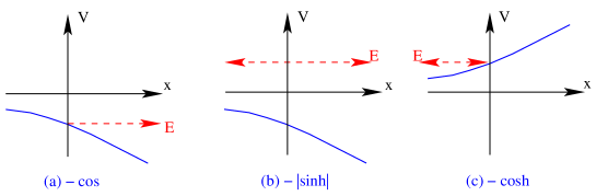
Figure 1: The various cases for motion in one dimension with an exponential potential, and the function $F$ appearing in their solution (23): (a) negative potential $V<0$ and negative energy $E<0$ yield $F=\cos$, (b) $V<0,\,E>0$ yield $F=|\sinh|$, (c) $V>0,\,E>0$ yield $F=\cosh$.

In our case (19) the potential is negative, and the energy is positive due to the constraint (18), so we are in case (b) of the figure. The most general solution is

$$A = A_{1}\,x+A_{0}$$

$$e^{-G} = \left|{1\over A_{1}}\,\sinh(A_{1}\,x)\right|~{},$$ (24)

where $x_{0}$ was set such that $e^{-G}$ vanishes at $x=0$, two other parameters $A_{0},\,A_{1}$ are displayed, and without loss of generality $A_{1}$ will be chosen to be positive from now on, just like $k$ was in (21).

Substituting this solution in the ansatz (1) using (5,14,16) we arrive at our final expression for the metric

$$ds^{2} = -e^{2A}\,dt^{2}+e^{-2A/(d-3)}\,\left[\exp\left({2(d-2)\over d-3}\,{\hat{G}}\right)\,dx^{2}+\exp\left({2\over d-3}\,{\hat{G}}\right)\,d\Omega^{2}_{d-2}\right]=$$

$$= ~{}\rule[-5.69054pt]{0.0pt}{22.76219pt}-e^{2(A_{1}x+A_{0})}\,dt^{2}+e^{-2(A_{1}x+A_{0})/(d-3)}\cdot$$

$$\cdot \left[\left({A_{1}\over(d-3)\,\sinh(A_{1}|x|)}\right)^{2(d-2)\over d-3}dx^{2}+\left({A_{1}\over(d-3)\,\sinh(A_{1}|x|)}\right)^{2\over d-3}d\Omega^{2}_{d-2}\right]~{}.$$

The first line stresses that if we consider a Kaluza-Klein reduction over $t$, then the $d-1$ Weyl rescaled metric (the Einstein frame) depends only on ${\hat{G}}$ and not on $A$. The 4d case is of special interest and the formulae simplify to

$$ds^{2}=-e^{2\,(A_{1}\,x+A_{0})}\,dt^{2}+e^{-2\,(A_{1}\,x+A_{0})}\,\left[\left({A_{1}\over\sinh(A_{1}|x|)}\right)^{4}\,dx^{2}+\left({A_{1}\over\sinh(A_{1}|x|)}\right)^{2}\,d\Omega^{2}_{d-2}\right]~{}.$$ (26)

Investigation of the metric. Let us compare this solution with the standard Schwarzschild solution

$$ds^{2}=-f\,dt^{2}+f^{-1}\,dr^{2}+r^{2}\,d\Omega^{2}_{d-2}$$

$$f=1-\left({r_{0}\over r}\right)^{d-3}~{}.$$ (27)

Since in this form $-g_{tt}|_{r\to\infty}=1$, and since $r\to\infty$ will be seen shortly to correspond to $x\to 0$, we must set $A_{0}=0$. Comparing $g_{\Omega\Omega}$ we find the change of variable $r=r(x)$ and transformation of the parameter $r_{0}=r_{0}(A_{1})$ to be

$$r^{d-3} = {2\,A_{1}\over(d-3)(1-\exp(-2\,A_{1}\,|x|))}$$ (28)

$$r_{0}^{~{}d-3} = {2\,A_{1}\over d-3}~{}.$$ (29)

Actually, one notices that the solution (A New Action-Derived Form of The Black Hole Metric) depends on $x$ only through the combination $y:=\exp(2\,A_{1}\,x)$ in terms of which it becomes

$$ds^{2} = -e^{2A_{0}}\,y\,dt^{2}+e^{-2A_{0}/(d-3)}\,\cdot$$

$$\cdot \left[\left({2\,A_{1}\over(d-3)\,(1-y)}\right)^{2\over d-3}{dy^{2}\over y\,(1-y)^{2}\,(d-3)^{2}}+\left({2\,A_{1}\over(d-3)\,(1-y)}\right)^{2\over d-3}\,d\Omega^{2}_{d-2}\right]$$

which is one step away from the standard form (27) through the use of the transformation rules (28).

Let us study the various regions in the coordinate $x$ using (28). $x=0$ is a singularity and it separates the $x$ axis into two regions: positive and negative $x$. For small $x$ on either side of $x=0$ ($A_{1}\,|x|\ll 1$) $r^{d-3}=[(d-3)|x|]^{-1}$ and we get flat space (Minkowski). As $x\to-\infty$ $g_{tt}\to 0$ and we reach a horizon, and thus negative $x$ represents the outer region of the black hole. More precisely, for $x\ll-1$, $x\propto\log(r-r_{0})$ and as such is asymptotically proportional to the standard “tortoise” coordinate $r^{*}$ (defined by $dr^{*}=dr/f(r)$). As $x\to+\infty$ $g_{tt}\to\infty$ (with no intermediate horizon) and thus positive $x$ describes a negative mass black hole. Finally, the inside of the black hole is not seen in these coordinates, since it requires a changes of signature for both $dx^{2},\,dt^{2}$. If one were to perform this change, the potential term in (12) would receive a minus sign, and that would change us from case (b) to case (c) in figure 1, changing accordingly all $\sinh$’s into $\cosh$’s in the formulae (A New Action-Derived Form of The Black Hole Metric,26).

Generalization and the charged black hole. The derivation above generalizes to any spherical black hole or black brane, the essential feature being for the metric to be of co-homogeneity 1. Let us demonstrate it for the case of the charged black hole (Reissner-Nordström).

We need to supplement the $A,B,\,C$ fields of the ansatz (1) with a vector potential $N_{\mu}$, and since we are interested in static, electrically charged black holes only $N_{0}$ is non-vanishing and so we may denote it simply by $N$. The action is taken to be the standard Einstein-Maxwell action

$$S=-\frac{1}{16\,\pi\,G}\int dV\left(R-\frac{1}{4}\,F_{\mu\nu}\,F^{\mu\nu}\right)$$ (31)

where $F_{\mu\nu}={\partial}_{\mu}N_{\nu}-{\partial}_{\nu}N_{\mu}$. In the static spherically symmetric case the action becomes

$$S_{p} = {\Omega_{d-2}\over 16\pi G}\,\int dt\,\int dx\,e^{A+B+(d-2)C}\cdot$$

$$\cdot \left[-e^{-2\,B}[2(d-2)\,A^{\prime}\,C^{\prime}+(d-2)(d-3)\,C^{\prime 2}]-(d-2)(d-3)\,e^{-2\,C}-{1\over 2}\,e^{-2\,A-2\,B}\,N^{\prime 2}\right]$$

We note that $N$ is an ignorable field. Therefore we continue to fix the gauge with (5) such that the kinetic term for $A,C$ will be canonical. The gauge-fixed action is

$$S=\int dx\left(\hat{A}^{2}-G^{2}-e^{2\,G}-{1\over 2}e^{-2\hat{A}}\,N^{\prime 2}\right)$$ (33)

where we define a shifted $A$ by

$$\hat{A}:=A-{1\over 2}\log{\frac{d-3}{d-2}}$$ (34)

and the constraint is

$$0=-\left.{{\partial}S_{p}\over{\partial}B}\right|_{B=A+(d-2)C}=\hat{A}^{2}+G^{2}-e^{2\,G}-{1\over 2}e^{-2\hat{A}}\,N^{\prime 2}~{}.$$ (35)

Since $N$ is an ignorable field, it is convenient at this point to transform into its conjugate momentum

$$Q=-e^{-2\hat{A}}\,N^{\prime}~{}.$$ (36)

$Q$ is conserved, and this can be considered a first integral of $N$’s equation of motion. A partial Legendre transform of $S$ with respect to $N$ yields after a multiplication by an overall minus sign

$$R=\hat{A}^{2}-G^{2}-e^{2\,G}+{1\over 2}e^{+2\hat{A}}\,Q^{2}$$ (37)

This action (37) decouples with respect to $\hat{A},G$, except for the constraint (35). The latter now reads

$$E_{A}=E_{G}$$ (38)

where we naturally define the $A,G$ energies to be

$$E_{A} := \hat{A}^{\prime 2}-{1\over 2}e^{2\hat{A}}\,Q^{2}$$

$$E_{G} := G^{\prime 2}-e^{2\,G}$$ (39)

Here we shall solve the equations of motion explicitly for the case of positive energies

$$E_{A}=E_{G}=A_{1}^{~{}2}$$ (40)

which will be seen to imply that the black hole is within the extremality limit.

The solution to the equations of motion is given by

$$e^{-\hat{A}} := \frac{Q}{\sqrt{2}\,A_{1}}\,\Big{|}\sinh\left(A_{1}(x-x_{A})\right)\Big{|}$$

$$e^{-G} := \frac{1}{A_{1}}\,\Big{|}\sinh(A_{1}x)\Big{|}$$ (41)

where $x_{A}$ is an arbitrary integration constant, and the analogous constant $x_{G}$ was set to zero without loss of generality due to invariance under $x$ translations. $N$ can be integrated from (36)

$$N=\frac{2\,A_{1}}{Q}\,\coth\left(A_{1}(x-x_{A})\right)+N_{0}~{}.$$ (42)

The standard Reissner-Nordström solution [6, 7, 4] is given by

$$ds^{2} = -f\,dt^{2}+f^{-1}\,dr^{2}+r^{2}\,d\Omega^{2}_{d-2}$$

$$f = 1-{2m\over r^{d-3}}+{q^{2}\over r^{2(d-3)}}$$

$$N = c\,{q\over r^{d-3}}+N_{0}$$ (43)

where $m,q$ are related to the mass and charge through some constants and in the current conventions $c=\sqrt{2(d-2)/(d-3)}$.

The relation between $x$ and the standard $r$ coordinate is given by

$$\frac{1}{r^{d-3}} = e^{A-{\hat{G}}}=\frac{\sqrt{(d-3)^{3}}}{\sqrt{d-2}}\,e^{\hat{A}-G}=\frac{\sqrt{2(d-3)^{3}}}{\sqrt{(d-2)}}\,\frac{1}{Q}\,\left|\frac{\sinh(A_{1}x)}{\sinh\left(A_{1}(x-x_{A})\right)}\right|=$$ (44)

$$= \frac{\sqrt{2(d-3)^{3}}}{\sqrt{d-2}}\,\frac{|\sinh(A_{1}\,x_{A})|}{Q}\,\Big{|}\coth\left(A_{1}(x-x_{A})\right)+\coth(A_{1}\,x_{A})\Big{|}$$

Let us map the various ranges of $x$ and $r$: assuming without loss of generality that $x_{A}\geq 0$ we have that while $-\infty\leq x\leq 0$ $r$ is in the range $r_{+}\leq r\leq+\infty$, while $0\leq x\leq x_{A}$ $r$ ranges over $+\infty\geq r\geq 0$ (a negative mass naked singularity), and while $x_{A}\leq x\leq+\infty$ $r$ is in the range $0\leq r\leq r_{-}$.

The relations between the 3 parameters $Q,A_{1},x_{A}$ (41) and the 2 standard parameters $q,m$ of (43) can be read by comparing the form of $g_{tt}$

$$-g_{tt}=e^{2A}=\left(\frac{A_{1}}{(d-3)\,\widetilde{Q}\,\sinh{(A_{1}\,x_{A})}}\right)^{2}\,\left[1-2\,\cosh{(A_{1}\,x_{A})}\frac{\widetilde{Q}}{r^{d-3}}+\left(\frac{\widetilde{Q}}{r^{d-3}}\right)^{2}\right]$$ (45)

where $\widetilde{Q}=\sqrt{(d-2)/(2(d-3)^{3})}\,Q$. In the standard form

$$1=\sqrt{-g}_{tt}|_{r\to\infty}=A_{1}/\left((d-3)\widetilde{Q}\sinh{(A_{1}\,x_{A})}\right)$$ (46)

and then by comparison

$$q = \widetilde{Q}$$

$$m = \cosh{(A_{1}\,x_{A})}\,\widetilde{Q}~{}.$$ (47)

In addition, we can use the third parameter to change the gravitational potential at infinity $g_{tt}|_{r\to\infty}$.

Open question. It would be interesting to see if similar action techniques can be of use in deriving black hole metrics with a higher dimension of co-homogeneity such as the co-homogeneity 2 rotating Kerr black hole.

Note added. In response to several messages which I received I would like to clarify a few points and relate to previous work.

The original motivation was to find an optimal analytical gauge to calculate the negative mode of the Schwarzschild black hole [8], and the current derivation appeared as a spin-off.

This derivation rests on the following two ideas: an action approach for a “maximally general ansatz” and a specific action-motivated gauge-fixing. This gauge fixing produces the current form of the metric (A New Action-Derived Form of The Black Hole Metric). None of these ideas is revolutionary: the action approach is not foreign to GR ever since the days of Hilbert [9] and Weyl [10], if not as common as in other branches of physics; and while the gauge fix is natural from the action perspective it is not impossible that another gauge will prove “equally natural”. Still, I found the combination appealing and since I had not seen such a derivation before, I decided to advertise it on the archives, and perhaps motivate further research along these lines.

I was informed that the current form of the metric (A New Action-Derived Form of The Black Hole Metric) did appear already in essence in [12]. While the methods of derivation share similarities being both action-based, they are still quite different. Our second form of the metric (A New Action-Derived Form of The Black Hole Metric) is closely related to [13], though the methods differ. Altogether however, judging by the correspondence which I received so far, it could very well be that the current derivation did not appear yet.

Acknowledgements

This research is supported in part by The Israel Science Foundation grant no 607/05 and by the Binational Science Foundation BSF-2004117.

References

- [1] K. Schwarzschild, “On The Gravitational Field Of A Mass Point According To Einstein’s Theory,” Sitzungsber. Preuss. Akad. Wiss. Berlin (Math. Phys. ) 1916, 189 (1916) [arXiv:physics/9905030].
- [2] J. W. York, “Role of conformal three geometry in the dynamics of gravitation,” Phys. Rev. Lett. 28, 1082 (1972).
- [3] G. W. Gibbons and S. W. Hawking, “Action Integrals And Partition Functions In Quantum Gravity,” Phys. Rev. D 15, 2752 (1977).
- [4] F. R. Tangherlini, “Schwarzschild field in n dimensions and the dimensionality of space problem,” Nuovo Cim. 27, 636 (1963).
- [5] L. D. Landau and E. M. lifshitz, “Mechanics,” Pergamon (1976), §41.
- [6] H. Reissner, “Über die Eigengravitation des elektrischen Felds nach den Einsteinschen Theorie,” Ann. Phys. bf 50, 106-120 (1916).
- [7] G. Nordström, “On the energy of the gravitational field in Einstein’s theory,” Proc. Kon. Ned. Akad. Wet. 20, 1238-1245 (1918).
- [8] B. Kol, “The Power of Action: The Derivation of the Black Hole Negative Mode,” arXiv:hep-th/0608001.
- [9] D. Hilbert, “Die Grundlagen der Physik (Zweite Mitteilung),” Nachr. Ges. Wiss. Go”ttingen, Math. Phys. K1., 53-76 (1917). An english translation is to be found in S. Antoci and D. E. Liebscher, “Reinstating Schwarzschild’s original manifold and its singularity,” arXiv:gr-qc/0406090.
- [10] H. Weyl, “Zur Gravitationstheorie”, Ann. Phys. 54, 117 (1917).
- [11] S. Deser and J. Franklin, “Schwarzschild and Birkhoff a la Weyl,” Am. J. Phys. 73, 261 (2005) [arXiv:gr-qc/0408067].
- [12] M. Cavaglia, “Two-dimensional reduced theory and general static solution for uncharged black p-branes,” Phys. Lett. B 413, 287 (1997), [arXiv:hep-th/9709055]. Eq (31).
- [13] M. Headrick and T. Wiseman, “Ricci flow and black holes,” arXiv:hep-th/0606086. Eq (A.5).