Non-linear Oscillations of Compact Stars and Gravitational Waves

Institute of Cosmology and Gravitation University of Portsmouth, UK Dr. M. Bruni First Reader Name Second Reader Name November, 2005

To my little flower Antonella

Abstract

This thesis investigates in the time domain a particular class of second order perturbations of a perfect fluid non-rotating compact star: those arising from the coupling between first order radial and non-radial perturbations. Radial perturbations of a non-rotating star, by themselves not emitting gravitational waves, produce a peculiar gravitational signal at non-linear order through the coupling with the non-radial perturbations. The information contained in this gravitational signal may be relevant for the interpretation of the astrophysical systems, e.g. proto-neutron stars and accreting matter on neutron stars, where both radial and non-radial oscillations are excited. Expected non-linear effects in these systems are resonances, composition harmonics, energy transfers between various mode classes.

The coupling problem has been treated by developing a gauge invariant formalism based on the 2-parameter perturbation theory (Sopuerta, Bruni and Gualtieri, 2004), where the radial and non-radial perturbations have been separately parameterized. Our approach is based on the gauge invariant formalism for non-radial perturbations on a time-dependent and spherically symmetric background introduced in Gerlach & Sengupta (1979) and Gundlach & M. García (2000). It consists of further expanding the spherically symmetric and time-dependent spacetime in a static background and radial perturbations and working out the consequences of this expansion for the non-radial perturbations. As a result, the non-linear perturbations are described by quantities which are gauge invariant for second order gauge transformations where the radial gauge has been fixed. This method enables us to set up a boundary initial-value problem for studying the coupling between the radial pulsations and both the axial (Passamonti et al.,2006) and polar (Passamonti at el., 2004) non-radial oscillations. These non-linear perturbations obey inhomogeneous partial differential equations, where the structure of the differential operator is given by the previous perturbative orders and the source terms are quadratic in the first order perturbations. In the exterior spacetime the sources vanish, thus the gravitational wave properties are completely described by the second order Zerilli and Regge-Wheeler functions.

The dynamical and spectral properties of the non-linear oscillations have been studied with a numerical code based on finite differencing methods and standard explicit numerical algorithms. The main initial configuration we have considered is that of a first order differentially rotating and radially pulsating star, where the initial profile of the stationary axial velocity has been derived by expanding in tensor harmonics the relativistic j-constant rotation law. For this case we have found a new interesting gravitational signal, whose wave forms show a periodic signal which is driven by the radial pulsations through the sources. The spectra confirm this picture by showing that the radial normal modes are precisely mirrored in the gravitational signal at non-linear perturbative order. Moreover, a resonance effect is present when the frequencies of the radial pulsations are close to the first $w$-mode. For the stellar model considered in this thesis the gravitational waves related to the fourth radial overtone is about three orders of magnitude higher than that associated with the fundamental mode. We have also roughly estimated the damping times of the radial pulsations due to the non-linear gravitational emission. These values radically depend on the presence of resonances. For a $10~{}ms$ rotation period at the axis and $15~{}km$ differential parameter, the fundamental mode damps after about ten billion oscillation periods, while the fourth overtone after ten only.

Notations and convenctions

• The signature of the metric is $\left(-,+,+,+\right)$, thus time-like 4-vectors have negative norms.

• The index notation of the tensor fields is the follows: Greek indices run from 0 to 3, capital Latin indices from 0 to 1, and small Latin indices from 3 to 4.

• In a tensor expression we use the Einstein’s sum convenction.

• The Eulerian perturbation fields for the first and second order perturbations are denoted with the notation of the 2-parameter perturbation theory. Therefore, the upper index (1,0) denotes first order radial perturbations, (0,1) the first order non-radial perturbation and (1,1) their coupling.

• In this thesis we have used the geometrical units in almost all the expressions. Thus, the speed of light and the gravitational constant are set $G=c=1$. Therefore, we have that:

  $$1~{}s = 2.9979\times 10^{5}~{}km\qquad\qquad\qquad$$

  $$1~{}g = 7.4237\times 10^{-24}~{}km$$

  $$M_{\odot} = 1.4766~{}km$$

Chapter 1 Introduction

Gravitational waves are the most elusive prediction of Einstein’s theory of gravity. The indirect evidence of their existence relies on the observations of the binary pulsar PSR 1913+16 (Hulse and Taylor [55]), that shows a decay of the orbital period consistent with the loss of angular momentum and energy due to the emission of gravitational waves. The prospect of starting a new astronomy based on gravitational radiation and providing a new corroboration of General Relativity has motivated many theoretical and experimental researches. As a result, the detection of gravitational waves seems feasible in the next decade by an international network of Earth-based laser interferometer detectors (LIGO, VIRGO, TAMA300, and GEO600) [3], bar resonant antennas (EXPLORER, AURIGA, NAUTILUS, ALLEGRO) [1] and by the Laser Interferometer Space Antenna (LISA) [2]. Three scientific runs have been so far carried out by the LIGO detectors, in collaboration with GEO and TAMA detectors for two of the three runs and with the bar detector ALLEGRO for the last run. The data analysis of the first and second science run sets upper limits on the gravitational signal emitted by a number of possible sources, such as stochastic background, coalescing binary stars, pulsars [4, 5, 6, 7, 10, 8]. The third science runs have been performed with a higher sensitivity and the data analysis leads to a significant improvement of the gravitational radiation upper limits [9]. Meanwhile, a second generation of detectors is already in the design stage for the exploration of the high frequency band, up to several kHz (advanced GEO600 [97], wide-band dual sphere detectors [21]), with an improvement of sensitivity up to two orders of magnitude with respect to the first-generation instruments.

Gravitational radiation could provide new information about the nature of astrophysical sources and help in the interpretation of the dynamical evolution of many such systems. Among the many sources of gravitational waves, the oscillations of compact stars are considered of great interest by astrophysicists and nuclear physicists. The extreme conditions present in the core of compact stars make them a unique laboratory, where nearly all the modern theoretical areas of research in physics can be tested.

In many astrophysical scenarios, compact stars may undergo oscillating phases. After violent events such as core collapse of a massive star, an accretion-induced-collapse of a white dwarf, or a binary white dwarf merger, the newly born protoneutron star is expected to pulsate non-linearly before various dissipative mechanisms damp the oscillations. Another system where pulsating phases may occur is a massive meta-stable compact object, which is born after the merger of a binary neutron star system. The gravitational signal emitted by the stellar oscillations lies in the high frequency band ($\nu\gtrsim 1kHz$) and strongly depends on the structure and physics of the star, for instance on the equation of state, rotation, crust, magnetic fields as well as on the presence of dissipative effects such as viscosity, shock formation, magnetic breaking, convective outer layers, etc. With a detailed analysis of the gravitational wave spectrum emitted by stellar pulsations we could infer through asteroseismology the fundamental parameters of neutron stars, such as mass, radius and rotation rate [14, 13]. This information is necessary for the nuclear physicists as they can test the equations of state proposed for the description of matter at supra-nuclear densities. However, the weakness of the gravitational signal and the noise associated with the location and technology of the detectors compels theorists to provide more and more accurate models to predict the spectral and wave form properties of the gravitational signal. These templates are indispensable for enhancing the chances of detection, by extracting the signal from the noise with statistical methods.

The spectral and dynamical properties of the oscillations of compact stars have been extensively investigated during the last forty years in Newtonian and Einstein theories of gravity. Linear perturbative techniques are appropriate for the analysis of small amplitude pulsations both in the frequency [109, 60] and the time domain approach [11, 96, 99, 98, 81]. In General Relativity, the oscillation spectrum of a compact object, such as black holes and neutron stars, is characterized by a discrete set of quasi-normal modes (QNM). These modes have complex eigenfrequencies whose real part describes the oscillation frequency, and the imaginary part the damping time due to the emission of gravitational waves. The classification of QNM is well known for a large set of stellar models and can be divided schematically in fluid and spacetime modes. The fluid modes have a Newtonian counterpart and can be sub-classified by the nature of the restoring force that acts on the perturbed fluid element. The spacetime modes are purely relativistic and are due to the dynamical role assumed by the spacetime in General Relativity (more details are given in chapter 3 and reference therein).

Rotating stars in General Relativity can be described with various approximations, such as the slow-rotation approximation [52] or recently with codes developed in numerical relativity [37]. The former approach is based on a perturbative expansion of the equations in powers of the dimensionless rotation parameter $\epsilon=\Omega/\Omega_{K}$, where $\Omega$ is the uniform angular rotation and $\Omega_{K}$ is the Keplerian angular velocity, which is defined as the frequency of a particle in stable circular orbit at the circumference of a star. The measured period of the fastest rotating pulsar corresponds to a relatively small rotation parameter $\epsilon\sim 0.3$, which may suggest that the slow rotation approximation provides an accurate description of rotating stars even for high rotation rates. However, in these cases the accuracy of this perturbative approach is different for the various physical stellar quantities. For instance, the quadrupole moment shows an accuracy to better than twenty percent, while the radius of the corotating and counterrotating innermost stable circular orbits is accurate to better than one percent [18]. Nevertheless, a protoneutron star may be expected to have a higher rotation rate that is not possible to describe with the slow rotation approximation. These regimes can be better addressed in numerical relativity by evolving the full set of non-linear Einstein equations [35, 105, 103]. Furthermore, recent works on the core collapse [33, 34], r-mode instability [94, 68, 71], accretion from a companion [40], or supernova fall back material [113], show that a neutron star manifests a degree of differential rotation.
These studies have clarified the effects of rotation on the dynamics of the oscillations, as well as showed the importance of using a relativistic treatment that takes into account the effects of the dragging of inertial frames. In particular, the presence in rotating stars of instabilities due to emission of gravitational waves has gained great attention. Almost all classes of oscillations of rotating stars, such as the f- and r-modes, are potentially unstable to the so-called Chandrasekhar- Friedman-Schutz (CFS) instability [24, 39]. This appears because beyond a critical value of the stellar angular velocity, a mode that in a corotating frame is retrograde and then has negative angular momentum, may appear moving forward in the inertial frame of a distant observer. As a result, this inertial observer will detect gravitational waves with positive angular momentum emitted by this mode. Thus, the gravitational radiation removes angular momentum by the retrograde mode by making it increasingly negative and then leading to instabilities. The losses of the angular momentum through gravitational waves slow down the star on secular timescales; eventually the star rotates slower than a critical value and the mode becomes stable. These instabilities could be strong sources of gravitational radiation and also limit the rotation rate of neutron stars, providing a possible explanation for the measured rotation period of pulsars. Many studies are currently dedicated to understand whether viscosity, magnetic fields, shock waves on the stellar surface or non-linear dynamics of oscillations may saturate this instability.

The non-linear analysis of stellar oscillations is more complex and only recently are some investigations being carried out, due to improvements achieved by the non-linear codes in numerical relativity [37]. Different methods have been used to investigate the properties of non-linear oscillations, such as for instance 3-dimensional general relativistic hydrodynamics code in Cowling or conformal flatness approximations [104, 35], a combination of linear perturbative techniques with general relativistic hydrodynamics simulations [114], or a new method where the non-linear dynamics is studied as a deviation from a background, which is described by a stellar equilibrium configuration [102]. These works, which have been dedicated to investigate the non-linear dynamics of different astrophysical systems: non-linear oscillations of a torus orbiting a black hole [114], non-linear axisymmetric pulsations of uniform and differential rotating compact stars [35] and non-linear radial oscillations of non-rotating relativistic stars [102], have revealed a new phenomenology associated with the non-linear regimes, the presence in the spectrum of non-linear harmonics. These harmonics arise from the coupling between different classes of linear modes or from non-linear self-couplings [102], and have a characteristic that could be appealing for the detection of gravitational waves: their frequencies appear as linear combinations of the linear oscillation modes. Therefore, some of these non-linear harmonics (sub-harmonics) can emerge at lower frequencies than the related linear modes, and then be within the frequency range where the detectors have higher sensitivity. However, since the amplitude of non-linear perturbations is usually the product of the amplitudes of first order perturbations, in order to have a detectable gravitational wave strain one needs non-linear effects that can enhance the gravitational signal, such as resonances, parameter amplifications or instabilities.
Strong non-linear regimes are adequately studied with a fully non-perturbative approach. However, many interesting physical effects of mild non-linear dynamics can be well addressed by second order perturbative techniques. An example is given by the analyses of black hole collisions in the so-called “close limit approximation”, where the second order perturbations of Schwarzschild black holes [46, 41] have provided accurate results even in non-linear regimes where the perturbative methods are expected to fail. Non-linear perturbative methods have been successfully used also for studying linear perturbations of rotating stars, where the rotation is treated perturbatively with the slow rotation approximation  [52, 103].
An important aspect of second order perturbative analyses is that of providing an estimate of the error associated with the first order treatment, as there is not an a priori method to determine the accuracy of the linear perturbative results. Thus, the convergence and the corrections associated with any term of the perturbative series can be determined only by investigating higher perturbative orders. Furthermore, non-linear perturbative equations are usually a system of partial differential equations, thus their numerical integration is computationally less expensive than the full Einstein equations which are treated in numerical relativity. This relative simplicity of the perturbative approach may then provide accurate results and can also be used to test the full non-linear simulations. However, an extension to second order perturbative investigations is not always straightforward [46, 41]. Some issues may arise from the identification of the physical quantities among the second order perturbative fields or from the movement of the stellar surface in non-linear stellar oscillations [101, 102].
In physical systems where the perturbative analysis can be described by more than a single parameter, as for stellar oscillations of a slowly rotating star or mode coupling between linear perturbations, the multi-parameter relativistic perturbation theory [19, 100] can help the interpretation of the gauge issues of non-linear perturbations. The identification of gauge invariant quantities allows us to have direct information about the physical properties of the system under consideration. The construction of such quantities is not in general simple, but recent works [83, 84] show how to build second order gauge-invariant perturbative fields from the knowledge of the associated first order gauge invariant perturbations. For a specific class of astrophysical systems a gauge invariant and coordinate independent formalism has been introduced nearly thirty years ago  [43, 45] for the analysis of one-parameter non-radial perturbations on a time dependent and spherically symmetric background. Recently, this formalism has been further developed [73, 48], and has been used to study non-radial perturbations on a collapsing star [51] and for linear perturbation on a static star [81].

The research project we have been working on aims to extend the perturbative analysis of compact stars at non-linear orders, in order to have a more comprehensive understanding of stellar oscillations and the related gravitational radiation. In particular, this thesis presents a gauge invariant formalism and a numerical code for studying the coupling between the radial and non-radial perturbations of a perfect fluid spherical star. The formalism for the polar perturbations has been worked out in a first paper [89]. The formalism and applications to axial perturbations are presented in [90]. Work in progress on the applications of the polar perturbative formalism will be presented in a future work. Radial and non-radial oscillations can be excited in the aftermath of a core collapse or by accreting matter on a neutron star. Radial perturbations of a non-rotating star are not damped by emission of gravitational radiation, but they can emit gravitational waves at non-linear order through the coupling with the non-radial perturbations. This picture changes in the presence of rotation, where the radial pulsations become sources of gravitational radiation and form a new class of modes, called quasi-radial modes. This coupling may be interesting for instance during a core bounce, where it is expected that an excitation prevalently of the quasi-radial and quadrupole modes. Even though the quadrupole component provides the dominant contribution to the gravitational radiation, the radial pulsations may store a considerable amount of kinetic energy and transfer a part of it to the non-radial perturbations. As a result, this non-linear interaction could produce a damping of the radial pulsations and an interesting gravitational signal. The strength of this signal depends naturally on the efficiency of the coupling, which is an effect worth exploring. In this thesis, we start to investigate this non-linear effect for small oscillations of a non-rotating star with the aim of including rotation in future works.
The polar coupling, i.e. between the radial and the polar sector of non-radial perturbations, is expected to be a priori more effective than the axial case. Indeed, the linear polar modes have a richer spectrum than the axial sector and from the values of the frequencies and the damping times of the fluid QNMs, the resonances and composition harmonics should be more probable between the polar fluid and the radial modes. However, for the purposes of this thesis we have implemented a numerical code for the axial coupling for mainly two reasons: i) the axial coupling can have interesting physical effects, ii) the perturbative equations are simpler and enable us to understand better the issues related to the numerical stability and accuracy of the code as well as the effects of the low density regions near the stellar surface on the non-linear simulations, etc.
When we consider the first order axial non-radial perturbations, we see that the only fluid perturbation is the axial velocity, which can be interpreted to describe a stationary differential rotation. Therefore, the linear axial gravitational signal does not have any dependence on the dynamics of the stellar matter. This picture changes at coupling order, where the differential rotation and first order metric perturbations can couple with the radial pulsations and source the axial gravitational waves. We will see in chapter 6 that this axial coupling produces a new class of quasi-radial modes, which can exist only for differentially rotating stars.

This thesis is organized in seven chapters. In chapter 2, we introduce the perturbative formalism used in this work, i.e. the multi-parameter relativistic perturbation theory and the gauge invariant formalism introduced by Gerlach and Sengupta and further developed by Gundlach and Martin Garcia (GSGM). In chapter  3, we describe the linear perturbations of a spherical star, i.e. the radial pulsations, the polar and axial non-radial perturbations. The equations for describing the coupling between the radial and axial and polar non-radial oscillations are presented in chapter 4, where in addition we discuss also the boundary conditions. In chapter 5, we present the proof of the gauge invariance of the perturbative tensor fields that describe the non-linear perturbations for this coupling. Chapter 6 is dedicated to the numerical code that simulates in the time domain the evolution of the coupling between the radial and axial non-radial perturbations. In this chapter we give all the technical details relating to the code and the results of the simulations. Finally in chapter 7, the conclusions and possible future developments are discussed.

The appendix has seven sections. We have reported the source terms of the equations derived by Gundlach and Martín García in section A. In section B, we write the full expressions of the sound wave equation for the fluid variable $H$, while in sections C and D we respectively present the source terms of the perturbative equations that describe the coupling between the radial pulsations and polar and axial non-radial perturbations. In addition, in section E we give the tensor harmonics, while some of the numerical methods used in the numerical code are given in sections F and G.

Chapter 2 Non-Linear Relativistic Perturbation Theory

Exact solutions of the equations of physics may be obtained for only a limited class of problems. This aspect is particularly present in General Relativity, where the complexity of the astrophysical systems and the non-linear Einstein field equations allows us to describe exactly only simplified and highly symmetric cases. Among various approximation techniques, perturbation methods are appropriate whenever the problem under consideration closely resembles one which is exactly solvable. It assumes that the difference from the exactly solvable configuration is small and that one may deviate from it in a gradual fashion. Deviations of the physical quantities from their exact solutions are referred to as perturbations. Analytically, this is expressed by requiring that the perturbation be a continuous function of a parameter, measuring the strength of the perturbation. Although perturbative techniques are more appropriate for small values of the perturbative parameter, sometimes they can give reliable results also for mildly non-linear regimes as shown for example in the analysis of black-hole collision [92]. Hence, in many cases the validity limit of perturbative methods cannot be determined a priori. A more accurate estimation can be reached by studying the convergence of the perturbative series, which then involves the analysis of the second or higher perturbative orders.

The gauge issue arises in General Relativity as in any other theory based on a principle of general covariance. The perturbative description of a physical system is not unique due to the presence of unphysical degrees of freedom related to the gauge, i.e. to the system of coordinates chosen for the analysis. This ambiguity can be eliminated either by fixing a particular gauge or by constructing perturbative variables which are invariant for any gauge transformation. In the former case, the properties and symmetries of the physical systems can help us to decide an appropriate gauge. In the latter approach, the identification of the gauge invariant fields is the difficult task.

In this section we review the perturbative framework we have used for investigating the coupling between the radial and non-radial perturbations. In section 2.1 we report the main results of the multi-parameter perturbation theory introduced by Bruni et al. [19] and Sopuerta et al. [100]. Section 2.2 is dedicated to the formalism introduced by Gerlach and Sengupta [43, 45], which has been further developed by Gundlach and M. Garcia [48], while in section 2.3 we outline the perturbative structure of our work which is based on the 2-parameter expansion of a static background.

2.1 Multi-parameter perturbation theory

Perturbation theory assumes the existence of two spacetimes, namely the background and perturbed spacetimes. The former is the spacetime described by an exact solution of the field equations, while the latter is the physical spacetime that the perturbation theory attempts to describe through the perturbation fields. The main requirement is that the physical description of the perturbed spacetime slightly deviates from that of the background solution.

Let us call $\mathcal{M}$ the spacetime manifold. The multi-parameter relativistic perturbation formalism assumes the existence of a smooth multi-parameter family of spacetime models which are diffeomorphic to the physical spacetime:

$$M_{\vec{\lambda}}=\left(\mathcal{M},\mathcal{T}_{\vec{\lambda}}\right)\,.$$ (2.1)

The quantity $\mathcal{T}_{\vec{\lambda}}$ represents a set of analytic tensor fields which are defined on $\mathcal{M}$ and that describe the physical and geometrical properties of the physical spacetime. The N-parameter vector $\vec{\lambda}\in\mathbb{R}^{N}$ labels any diffeomorphic representation of the physical spacetime $M_{\vec{\lambda}}$, and controls the deviation from the background quantities due to the contribution of the various perturbative parameters of the system under consideration. In this notation the background manifold $M_{b}$ is then identified with the spacetime model $M_{b}\equiv M_{\vec{0}}$. Furthermore, the validity of the Einstein field equations is assumed on any manifold $M_{\vec{\lambda}}$:

$$E\left(\mathcal{T}_{\vec{\lambda}}\right)=0\,.$$ (2.2)

In a perturbative approach, the comparison of perturbed and background variables is crucial for determining the accuracy of the perturbative description. In a physical theory based on a principle of general covariance as in General Relativity, this procedure requires a more precise definition that takes into account the gauge issue. Let us for instance consider a relation commonly used in perturbation theory,

$$\mathcal{T}_{\vec{\lambda}}\left(q\right)=\mathcal{T}_{b}\left(p\right)+\delta\mathcal{T}_{\vec{\lambda}}\left(p\right)\,,\qquad\textrm{where}\quad\delta\mathcal{T}_{\vec{\lambda}}\ll\mathcal{T}_{b}\,.$$ (2.3)

Here, $q$ and $\mathcal{T}_{\vec{\lambda}}$ are respectively a point and a tensor field in the perturbed manifold $M_{\vec{\lambda}}$, while the point $p$ and the tensors $\mathcal{T}_{b}$ and $\delta\mathcal{T}_{\vec{\lambda}}$ belong to the background $M_{b}$. From equation (2.3) the tensor $\mathcal{T}_{\vec{\lambda}}\left(q\right)$ can be considered as a small deviation of the background value $\mathcal{T}_{b}$. However, we can notice that the perturbed and the background tensors are applied at points belonging to different manifolds. Therefore, in order to have a well posed relation it is necessary to establish a correspondence between these two points $p$ and $q$ and consequently between the three tensor fields in the expression (2.3). This point identification between the various representations of the physical spacetime $M_{\vec{\lambda}}$ is provided by a N-parameter group of diffeomorphisms $\mathcal{D}_{\varphi}=\left\{\varphi_{\vec{\lambda}}:\vec{\lambda}\in\mathbb{R}^{N}\right\}$,

$$\varphi:\mathcal{M}\times\mathbb{R}^{N} \rightarrow \mathcal{M}$$ (2.4)

$$(p,\vec{\lambda}) \mapsto \varphi(p,\vec{\lambda})\equiv\varphi_{\vec{\lambda}}(p)\,,$$

where the identity element corresponds to the null vector $\vec{\lambda}=\vec{0}$, i.e. $\varphi_{\vec{\lambda}}(p)=p$. The choice of the identification map $\varphi$ is completely arbitrary and in perturbation theory this arbitrariness is called “gauge freedom”. It is worth noticing that the gauge issue in perturbation theory is in general independent on the gauge related to the background spacetime, which fixes the system of coordinates only on the background manifold $M_{\,b}$. In order to have a correct description of a physical system the physical observables have to be isolated from the gauge degrees of freedom. This can be accomplished by fixing a particular gauge, where the variables assume the correct physical meaning, or alternatively by determining a set of gauge invariant quantities. The latter procedure can be more difficult to realize, but it provides directly the physical quantities of the system.

2.1.1 Taylor expansion

A perturbative solution of the Einstein equations is built as a correction of the background solution. This property, expressed in equation (2.3), allows us to approximate the physical variables and the field equation by their Taylor series. However, in order to define correctly a relativistic multi-parameter Taylor expansion some concepts related to the properties of the N-parameter group of diffeomorphisms have to be specified.

In general, a consistent perturbative scheme should not depend on the order followed for performing two or more perturbations. We can then consider an Abelian group of diffeomorphisms which is defined by equation (2.4) and the following composition rule:

$$\varphi_{\vec{\lambda}}\circ\varphi_{\vec{\lambda^{\prime}}}=\varphi_{\vec{\lambda}+\vec{\lambda^{\prime}}}\quad\textrm{for}\quad\forall\,\vec{\lambda},\vec{\lambda^{\prime}}\in\mathbb{R}^{N}\,.$$ (2.5)

Therefore, we can decompose every diffeomorphism $\varphi_{\vec{\lambda}}$ as a product of N one-parameter diffeormorphisms:

$$\varphi_{\vec{\lambda}}=\varphi_{(\lambda_{1},0,..,0)}\circ\cdot\cdot\cdot\cdot\circ~{}\varphi_{(0,..,0,\lambda_{N})}\,.$$ (2.6)

It is also evident from the previous property and the commutation rules that there are $N!$ equivalent decompositions of the diffeomorphism $\varphi_{\vec{\lambda}}$. In any point of the perturbed manifold $M_{\vec{\lambda}}$, a diffeomorphism $\varphi_{\vec{\lambda}}$ defines a N-parameter flow $\varphi_{\vec{\lambda}}(p)$. This flow is generated by a vector field $\vec{\zeta}\in\mathbb{R}^{N}$ that acts on the tangent space of $M_{\vec{\lambda}}$. In an Abelian group the generators of two different flows commute $\left[\vec{\zeta},\vec{\zeta}^{\prime}\right]=0$ and a N-dimensional basis with the N independent vectors can be defined:

$$\left\{\vec{\zeta}_{k}\right\}_{k=1..N}\,,\qquad\textrm{where}\quad\vec{\zeta}_{k}=\left(0,..,\zeta_{k},..0\right)\,.$$ (2.7)

This basis generates the N one-parameter groups of diffeomorphisms of equation (2.6) and can be used to decompose the vector field $\vec{\zeta}$ in its N components

$$\vec{\zeta}=\sum_{k=1}^{N}\vec{\zeta}_{k}\quad\textrm{where}\quad\vec{\zeta}_{k}=\left(0,..,\zeta_{k},..0\right)\,,$$ (2.8)

and to define the Lie derivative of an arbitrary tensor field $\mathcal{T}$

$$\pounds_{\vec{\zeta}_{k}}\mathcal{T}=\left.\frac{\partial\varphi^{\ast}_{\vec{\lambda}_{k}}\mathcal{T}}{\partial\lambda_{k}}\right|_{\lambda_{k}=0}\quad\textrm{where}\quad\vec{\lambda}_{k}=(0,..,\lambda_{k},..,0)\,.$$ (2.9)

The operator $\varphi^{\ast}_{\vec{\lambda}_{k}}$ is the pull-back associated with the flow $\varphi_{\vec{\lambda}_{k}}$.

The Taylor expansion of the pull-back $\varphi^{\ast}_{\vec{\lambda}_{k}}$ around the parameter $\vec{\lambda}=\vec{0}$ is then defined as follows:

$$\varphi^{\ast}_{\vec{\lambda}_{k}}\mathcal{T}=\sum_{n\geq 0}\frac{\lambda^{n}_{k}}{n!}~{}\pounds_{\vec{\zeta}_{k}}^{n}\mathcal{T}\equiv\exp{\left(\lambda_{k}\pounds_{\vec{\zeta}_{k}}\mathcal{T}\right)}\,.$$ (2.10)

The last equality in equation (2.10) is a formal definition that will be very useful later for carrying out calculations with the Baker-Campbell-Hausdorff (BCH) formula. The definition (2.10) and the diffeomorphism decomposition expressed in equation (2.6) allows us to define the Taylor expansion associated with the diffeomorphism $\varphi_{\vec{\lambda}}$:

$$\varphi^{\ast}_{\vec{\lambda}}\mathcal{T}=\sum_{n_{1}..n_{N}\geq 0}\left(\prod_{p=1}^{N}\frac{\lambda^{n_{p}}_{p}}{n_{p}!}~{}\pounds_{\vec{\zeta}_{p}}^{n_{p}}\right)\mathcal{T}\equiv\exp{\left(\sum_{p=1}^{N}\lambda_{p}~{}\pounds_{\vec{\zeta}_{p}}\right)}\mathcal{T}$$ (2.11)

2.1.2 Perturbations

In a particular gauge, the exact perturbations of a generic tensor field $\mathcal{T}$ are defined as follows:

$$\Delta\mathcal{T}_{\vec{\lambda}}^{\varphi}\equiv\varphi^{\ast}_{\vec{\lambda}}\mathcal{T}_{\vec{\lambda}}-\mathcal{T}_{\vec{0}}\,,$$ (2.12)

where the tensors $\Delta\mathcal{T}_{\vec{\lambda}}^{\varphi}$ and $\varphi^{\ast}_{\vec{\lambda}}\mathcal{T}_{\vec{\lambda}}$ as well as the background tensor $\mathcal{T}_{b}$ are defined on the background spacetime $M_{b}$. The definition (2.12) indicates that the background $M_{b}$ is the fundamental spacetime where all the perturbative fields are transported by the N-parameter flows and then compared with the background fields. The definition (2.12) can be rewritten by using the Taylor expansion (2.11) in the following form

$$\Delta\mathcal{T}_{\vec{\lambda}}^{\varphi}\equiv\sum_{n_{1},..,n_{N}\geq 0}\left(\prod_{p=1}^{N}\frac{\lambda_{p}^{n_{p}}}{n_{p}!}\right)\delta_{\varphi}^{\vec{n}}\mathcal{T}-\mathcal{T}_{b}\,,$$ (2.13)

where the vector $\vec{n}=\left(n_{1},..,n_{N}\right)$ controls the perturbation order of a tensor field with respect to the N-parameter,

$$\delta_{\varphi}^{\vec{n}}\mathcal{T}\equiv\frac{\partial^{n_{T}}\varphi^{\ast}_{\vec{\lambda}}T}{\partial\lambda_{1}^{n_{1}}..\lambda_{N}^{n_{N}}}=\prod_{p=1}^{N}\pounds_{\zeta_{p}^{n_{p}}}\mathcal{T}\,,$$ (2.14)

and $n_{T}=\sum_{p=1}^{N}n_{p}$ is the total perturbation order.

2.1.3 Gauge transformations

The representation of a perturbative field in the background manifold depends in general on the gauge choice $\varphi_{\vec{\lambda}}$. Let consider two generic gauges represented by the diffeomorphisms $\varphi$ and $\psi$, which are generated respectively by the vector fields $\left({}^{\varphi}\zeta_{1},..,{}^{\varphi}\zeta_{N}\right)$ and $\left({}^{\psi}\zeta_{1},..,{}^{\psi}\zeta_{N}\right)$. A gauge transformation is then defined by a diffeomorphism

$$\Phi_{\vec{\lambda}}:\mathcal{M}\rightarrow\mathcal{M}$$ (2.15)

that for a given $\vec{\lambda}$, connects the physical descriptions determined in the two gauges $\varphi$ and $\psi$ as follows:

$$\Phi:\equiv\varphi_{\vec{\lambda}}^{-1}\circ\psi_{\vec{\lambda}}=\varphi_{-\vec{\lambda}}\circ\psi_{\vec{\lambda}}\,.$$ (2.16)

The family of all diffeomorphisms that relate two gauges does not form in general a group,

$$\Phi:\mathcal{M}\times\mathbb{R}^{N} \rightarrow \mathcal{M}$$ (2.17)

$$(p,\vec{\lambda}) \mapsto \Phi(p,\vec{\lambda})\equiv\Phi_{\vec{\lambda}}(p)\,.$$

Since the gauge transformation $\Phi_{\vec{\lambda}}$ is a diffeomorphism we can extend to it some definitions used in the previous sections for the identification maps. For instance, the pull-back $\Phi_{\vec{\lambda}}^{\ast}$ of a generic tensor field $\mathcal{T}$ induced by the gauge transformation (2.16) can be defined by using the expression (2.11) in the following way:

$$\Phi_{\vec{\lambda}}^{\ast}\mathcal{T} = (\varphi_{-\vec{\lambda}}\circ\psi_{\vec{\lambda}})^{\ast}\mathcal{T}=\psi_{\vec{\lambda}}^{\ast}\circ\varphi_{-\vec{\lambda}}^{\ast}\mathcal{T}$$ (2.18)

$$= \exp{\left(\sum_{P=1}^{N}\lambda_{P}\pounds_{{}^{\psi}\zeta_{P}}\right)}\exp{\left(-\sum_{P=1}^{N}\lambda_{P}\pounds_{{}^{\varphi}\zeta_{P}}\right)}\mathcal{T}\,.$$

The gauge transformation $\Phi_{\vec{\lambda}}$ is generated by the vector field $\xi_{\vec{n}}$, which can be in general expressed in terms of the two generators of the gauge transformation $\varphi$ and $\psi$. In [100], the authors derive the relations between these gauge generators as well as among the perturbation fields by using the Baker-Campbell-Hausdorff (BCH) formula, which for two linear operators $A,B$ is so defined:

$$e^{A}e^{B}=e^{f(A,B)}\,,$$ (2.19)

where the functional $f(A,B)$ is given by,

$$f(A,B)=\sum_{m\geq 1}^{\infty}\frac{(-1)^{m-1}}{m}\sum_{\begin{array}[]{c}p_{i},q_{i}\\ p_{i}+q_{i}\geq 1\end{array}}\frac{[\overbrace{A\cdots A}^{p_{1}}\overbrace{B\cdots B}^{q_{1}}\cdots\overbrace{A\cdots A}^{p_{m}}\overbrace{B\cdots B}^{q_{m}}]}{\left[\sum_{\alpha=1}^{m}(p_{j}+q_{j})\right]\prod_{\alpha=1}^{m}p_{\alpha}!q_{\alpha}!}\,,$$ (2.22)

and where in the previous expression the following notation for the commutation operators has been used $\left[X_{1}X_{2}X_{3}\cdot\cdot X_{n}\right]\equiv\left[\cdot\cdot\cdot\left[\left[X_{1},X_{2}\right],X_{3}\right],\cdot\cdot\cdot,X_{n}\right]$. By using the BCH formula, the gauge transformation (2.18) reduces to a single exponential operator,

$$\Phi_{\vec{\lambda}}^{\ast}\mathcal{T}=\exp{\left\{\sum_{n_{1},..,n_{N}\geq 0}\left(\prod_{p=1}^{N}\frac{\lambda_{p}^{n_{p}}}{n_{p}!}\right)\pounds_{\xi_{\vec{n}}}-\mathcal{I}\right\}}\mathcal{T}\,,$$ (2.23)

where $\mathcal{I}\equiv\pounds_{\vec{0}}$ is the identity operator.

The gauge transformations at every perturbative order are then determined with the following procedure:
i) by using the definition (2.16), one defines a new relation between the pull-backs $\varphi_{\vec{\lambda}}^{\ast}\mathcal{T}$ and $\psi_{\vec{\lambda}}^{\ast}\mathcal{T}$:

$$\psi_{\vec{\lambda}}^{\ast}\mathcal{T}_{\vec{\lambda}}=\Phi_{\vec{\lambda}}^{\ast}\varphi_{\vec{\lambda}}^{\ast}\,\mathcal{T}_{\vec{\lambda}}\,.$$ (2.24)

ii) Thus, one can expand equation (2.24) by using the expressions (2.11) and (2.23). In doing that, one can use the linearity of the functional $f(A,B)$ on the operators $A$ and $B$ and their commutators, and also the linearity of the operators $A,B$ on the respective Lie derivatives. iii) At the end, the desired relations can be determined by comparing the terms order by order (for more details see [100]).

In case of 2-parameter perturbations $N=2$, which is the parameter number used in this thesis, the gauge transformations at first order are the well known relations:

$$\delta_{\psi}^{(1,0)}\mathcal{T} = \delta_{\varphi}^{(1,0)}\mathcal{T}+\pounds_{\xi_{(1,0)}}\mathcal{T}_{b}\,,$$ (2.25)

$$\delta_{\psi}^{(0,1)}\mathcal{T} = \delta_{\varphi}^{(0,1)}\mathcal{T}+\pounds_{\xi_{(0,1)}}\mathcal{T}_{b}\,.$$ (2.26)

At second order, the perturbation fields in the two gauges are related as follows:

$$\delta_{\psi}^{(2,0)}\mathcal{T} = \delta_{\varphi}^{(2,0)}\mathcal{T}+2\pounds_{\xi_{(1,0)}}\delta_{\varphi}^{(1,0)}\mathcal{T}+\left(\pounds_{\xi_{(2,0)}}+\pounds_{\xi_{(1,0)}}^{2}\right)\mathcal{T}_{b}\,,$$ (2.27)

$$\delta_{\psi}^{(0,2)}\mathcal{T} = \delta_{\varphi}^{(0,2)}\mathcal{T}+2\pounds_{\xi_{(0,1)}}\delta_{\varphi}^{(0,1)}\mathcal{T}+\left(\pounds_{\xi_{(0,2)}}+\pounds_{\xi_{(0,1)}}^{2}\right)\mathcal{T}_{b}\,,$$ (2.28)

$$\delta_{\psi}^{(1,1)}\mathcal{T} = \delta_{\varphi}^{(1,1)}\mathcal{T}+\pounds_{\xi_{(1,0)}}\delta_{\varphi}^{(0,1)}\mathcal{T}+\pounds_{\xi_{(0,1)}}\delta_{\varphi}^{(1,0)}\mathcal{T}$$ (2.29)

$${}+\left[\pounds_{\xi_{(1,1)}}+\left\{\pounds_{\xi_{(1,0)}},\pounds_{\xi_{(0,1)}}\right\}\right]\mathcal{T}_{b}\,,$$

where $\left\{\cdot,\cdot\right\}$ is the anticommutator. Gauge transformations for higher perturbative orders can be found in reference [19].

2.2 Gauge invariant perturbative formalism (GSGM)

Linear perturbations on a spherically symmetric background can be well described by using the formalism of Gerlach and Sengupta [43, 45]. With a 2+2 decomposition of the spacetime, the authors set up a covariant formalism to study linear non-radial perturbations on a time dependent and spherically symmetric background. Gundlach and Martín–García have further developed this formalism for a self-gravitating perfect fluid [73, 48, 74]. The authors have specified a general fluid frame on which all the tensor fields and perturbative equations can be decomposed. This approach leads to a set of scalar gauge invariant fields and equations, which are easily adaptable to any coordinate system of the background. Hereafter we refer to this formalism with the acronym GSGM.

2.2.1 The time dependent background

The background manifold is a warped product $M^{2}\times S^{2}$ of a two dimensional Lorentzian manifold $M^{2}$ and the 2-sphere $S^{2}$. The metric can be written as the semidirect product of a general Lorentzian metric on $M^{2}$, $g_{AB}$, and the unit curvature metric on $S^{2}$, that we call $\gamma_{ab}$:

$$\mbox{g}_{\alpha\beta}=\left(\begin{array}[]{cc}\mbox{g}_{AB}&0\\ 0&r^{2}\gamma_{ab}\end{array}\right)\,.$$ (2.30)

With Greek letters we denote the components defined in the 4-manifold, whereas the capital and small latin letters describe respectively the tensors in the $M^{2}$ and $S^{2}$ sub-manifolds. The scalar function $r=r(x^{A})$ is defined in $M^{2}$, and can be chosen as the invariantly defined radial (area) coordinate of spherically-symmetric spacetimes. Besides the covariant derivative in the four dimensional spacetime, defined as usual

$$g_{\alpha\beta;\mu}=0\,,$$ (2.31)

we can introduced in the two submanifolds two distinct covariant derivatives

$$g_{AB|C}=0\,,\qquad\gamma_{ab:c}=0\,,$$ (2.32)

where the vertical bar corresponds to the covariant derivative of $M^{2}$ and the semicolon to that of the 2-sphere $S^{2}$. Moreover, we can introduce the completely antisymmetric covariant unit tensors on $M^{2}$ and on $S^{2}$, $\epsilon_{AB}$ and $\epsilon_{ab}$ respectively, in such a way that they satisfy:

$$\epsilon_{AB|C}=\epsilon_{ab:c}=0\,,\qquad\epsilon_{AC}\epsilon^{BC}=-g_{A}^{B}\,,\qquad\epsilon_{ac}\epsilon^{bc}=\gamma_{a}^{b}\,.$$ (2.33)

The energy-momentum tensor in a spherically symmetric spacetime has the same block diagonal structure as the metric,

$$T_{\alpha\beta}=\textrm{diag}\left(\ t_{AB}\;,\,r^{2}Q(x^{C})\gamma_{ab}\right)\,,$$ (2.34)

where $Q(x^{C})$ is a function defined on $M^{2}$. In this thesis we have used a perfect-fluid description of the stellar matter, thus we specialize the GSGM formalism to this case. Therefore, we have for $T_{\alpha\beta}$,

$$T_{\alpha\beta}=(\rho+p)u_{\alpha}u_{\beta}+pg_{\alpha\beta}\,,$$ (2.35)

where $\rho$ and $p$ are the mass-energy density and pressure, and $u_{\alpha}$ is the fluid velocity. The background fluid velocity in spherical symmetry has vanishing tangential components,

$$u_{\alpha}=(u_{A},0)\,.$$ (2.36)

The velocity $u_{A}$ and the space-like vector

$$n_{A}\equiv-\epsilon_{AB}u^{B}~{}~{}~{}\Rightarrow~{}~{}~{}n_{A}u^{A}=0\,,$$ (2.37)

provide an orthonormal two dimensional basis $\left\{u_{A},n_{B}\right\}$ for the submanifold $M^{2}$.

The metric $\mbox{g}_{AB}$ and the completely antisymmetric tensor $\epsilon_{AB}$ can be written in terms of these frame vectors as follows

$$g_{AB}=-u_{A}u_{B}+n_{A}n_{B}\,,~{}~{}~{}~{}\qquad\epsilon_{AB}=n_{A}u_{B}-u_{A}n_{B}\,,$$ (2.38)

while the energy-momentum tensor assumes the following form

$$t_{AB} = \rho u_{A}u_{B}+pn_{A}n_{B}\,,~{}~{}~{}~{}Q=p\,.$$ (2.39)

In any given coordinate system for $M^{2}$, $\{x^{A}\}\,,$ one can define the following quantity:

$$v_{A}\equiv\frac{1}{r}r_{|A}\,.$$ (2.40)

Then, any covariant derivative on the spacetime can be written in terms of the covariant derivatives on $M^{2}$ and $S^{2}$, plus some terms due to the warp factor $r^{2}$, which can be written in terms of $v_{A}$. The frame derivatives of a generic scalar function $f$ are defined by

$$\dot{f}\equiv u^{A}f_{|A}\,,\qquad f^{\prime}\equiv n^{A}f_{|A}\,,$$ (2.41)

which obey the following commutative relation:

$$(\dot{f}~{})^{\prime}-(f^{\prime}~{})\dot{}=\mu f^{\prime}-\nu\dot{f}\,.$$ (2.42)

Furthermore, a set of background scalars are introduced in order to write the background and perturbative equations in a scalar form:

$$\Omega\equiv\ln\rho,\quad U\equiv u^{A}v_{A},\quad W\equiv n^{A}v_{A},\quad\mu\equiv u^{A}_{~{}|A},\quad\nu\equiv n^{A}_{~{}|A}\,.$$ (2.43)

Finally, the Einstein field equation for the background spacetime

$$R_{{\alpha}\beta}-\frac{R}{2}g_{{\alpha}\beta}=8\pi T_{{\alpha}\beta}$$ (2.44)

in the 2+2 split are given by the following equations:

$$-2\left(v_{A\mid B}+v_{A}v_{B}\right)+\left(2v_{C}^{~{}\mid C}+3v_{C}v^{C}-\frac{1}{r^{2}}\right)g_{AB} = 8\pi t_{AB}\,,$$ (2.45)

$$v_{C}^{~{}\mid C}+v_{C}v^{C}-R = 8\pi Q\,,$$ (2.46)

where $R=\frac{1}{2}R^{A}_{A}$ is the Gauss curvature of $M^{2}$. The conservation of the energy-momentum tensor

$$T^{{\alpha}\beta}_{~{}~{}~{}~{};{\alpha}}=0\,$$ (2.47)

leads to the energy conservation equation and to the relativistic generalization of the Euler equation:

$$\dot{\Omega}+\left(1+\frac{p}{\rho}\right)\left(\mu+2U\right) = 0\,,$$ (2.48)

$$c_{s}^{2}\Omega^{\prime}+\left(1+\frac{p}{\rho}\right)\nu = 0\,,$$ (2.49)

and $c_{s}^{2}$ is the speed of sound defined on the isentropic fluid trajectories as follows:

$$c_{s}^{2}=\left.\frac{\partial p}{\partial\rho}\right|_{s}\,.$$ (2.50)

2.2.2 Perturbations

Linear perturbations of a spherically-symmetric background can be decomposed in scalar, vector and tensor spherical harmonics. The perturbative variables are then completely decoupled in a part depending on the angular coordinates of the 2-sphere and a part defined on the submanifold $M^{2}$. This expansion is really helpful because the perturbative problem is reduced to a 2-dimensional problem, usually a time and spatial coordinate. The tensor harmonics are decomposed in two different classes of basis, the so-called polar (even) parity and axial (odd) parity tensor harmonics. These transform differently under a parity transformation, namely as $(-1)^{l}$ for the polar and as $(-1)^{l+1}$ for the axial.

The basis for scalar function is given by the scalar spherical harmonics $Y^{lm}$, which are eigenfunctions of the covariant Laplacian on the sphere:

$$\gamma^{ab}Y^{lm}_{:ab}=-l(l+1)Y^{lm}\,.$$ (2.51)

where the integers $(l,m)$ are respectively the multipole index and the azimuthal number. For a given $l$, the azimuthal number can assume the following $2l+1$ values:

$$-l,\,-l+1,\,..0..\,l-1,\,l\,.$$

There is not any axial basis for the scalar case. A basis of vector spherical harmonics (defined for $l\geq 1$) is

$$Y^{lm}_{a} \equiv Y^{lm}_{:a}\qquad\quad\textrm{polar}\,,$$ (2.52)

$$S^{lm}_{a} \equiv \epsilon_{a}^{~{}b}Y^{lm}_{b}\qquad\textrm{axial}\,,$$ (2.53)

A basis of tensor spherical harmonics (defined for $l\geq 2$) for the polar case is given by

$$Y_{ab}^{lm}\equiv Y^{lm}\gamma_{ab}\,,\qquad Z^{lm}_{ab}\equiv Y^{lm}_{:ab}+\frac{l(l+1)}{2}Y^{lm}\gamma_{ab}\,,$$ (2.54)

and for the axial class by the following definition:

$$S^{lm}_{ab}\equiv S^{lm}_{a:b}+S^{lm}_{b:a}\,,$$ (2.55)

The explicit form of the tensor harmonics are given in appendix E.

The perturbations of the covariant metric and energy-momentum tensors can be expanded in the polar basis as

$$\delta g^{pol}_{\alpha\beta} = \left(\begin{array}[]{cc}h_{AB}^{lm}\,Y^{lm}&h_{A}^{pol~{}lm}\,Y^{lm}_{a}\\ \\ h_{A}^{pol~{}lm}\,Y^{lm}_{a}&\ r^{2}(K^{lm}\,\gamma_{ab}\,Y^{lm}+G^{lm}\,Y_{:ab}^{lm})\\ \end{array}\right)\,,$$ (2.59)

$$\delta t_{\alpha\beta}^{pol} = \left(\begin{array}[]{cc}\delta t_{AB}^{lm}\,Y^{lm}&\delta t_{A}^{pol~{}lm}\,Y^{lm}_{a}\\ \\ \delta t_{A}^{pol~{}lm}\,Y^{lm}_{a}&\ r^{2}\,\delta t^{3\,lm}\,\gamma_{ab}\,Y^{lm}+\delta t^{2\,lm}\,Z_{ab}^{lm}\\ \end{array}\right)\,,$$ (2.63)

and axial basis as

$$\delta g_{\alpha\beta}^{ax} = \left(\begin{array}[]{cc}0&h_{A}^{ax~{}lm}\,S^{lm}_{a}\\ \\ h_{A}^{ax~{}lm}\,S^{lm}_{a}&\ h\left(S_{a:b}^{lm}+S_{b:a}^{lm}\right)\\ \end{array}\right)\,,$$ (2.67)

$$\delta t_{\alpha\beta}^{ax} = \left(\begin{array}[]{cc}0&\delta t_{A}^{ax~{}lm}\,S^{lm}_{a}\\ \\ \delta t_{A}^{ax~{}lm}\,S^{lm}_{a}&\ \delta t^{lm}\,\left(S_{a:b}^{lm}+S_{b:a}^{lm}\right)\\ \end{array}\right)\,.$$ (2.71)

In a spherically symmetric background the axial and polar perturbations are dynamically independent, and for a given multipole index $l$ their dynamics does not depend on the value of the azimuthal number $m$. For simplicity, we can then study the non-radial perturbations on a spherical star by only considering the axisymmetric case $m=0$. This approximation is not valid for instance in a rotating configuration, where axisymmetric and non-axisymmetric perturbations have different spectral and dynamical features.

The true degrees of freedom on metric and matter perturbations can be determined by a set of gauge-invariant variables. In one parameter perturbation theory, see section 2.1.3, the first order perturbation $\delta\mathcal{T}$ of a generic tensor field $\mathcal{T}$ is gauge-invariant if and only if the following condition is satisfied [106]:

$${\cal L}_{\xi}\mathcal{T}_{b}=0\,,$$ (2.72)

where $\mathcal{T}_{b}$ is the value of $\mathcal{T}$ on the background spacetime and $\xi$ is an arbitrary vector field that generates the gauge transformation (see section 2.1.3 and reference [106]). By combining separately the polar perturbation fields $h_{AB},\,h^{pol}_{A},\,K,\,G$, $\delta t_{AB},\,\delta t_{A},\,\delta t^{2},\,\delta t^{3}\,,$ and the axial ones $h_{A}^{ax},\,h$, $\delta t^{ax}_{A},\,\delta t\,$, it is possible to determined the following set of gauge-invariant variables [43, 45], where for clarity the harmonic indices $(l,m)$ are neglected,
polar

$$k_{AB} = h_{AB}-(p_{A|B}+p_{B|A})\,,$$ (2.73)

$$k = K-2v^{A}p_{A}\,,$$ (2.74)

$$T_{AB} = \delta t_{AB}-t_{AB|C}\,p^{C}-t_{AC}\,p^{C}_{|B}-t_{BC}\,p^{C}_{|A}\,,$$ (2.75)

$$T^{3} = \delta t^{3}-p^{C}(Q_{|C}+2Qv_{C})+\frac{l(l+1)}{2}\,Q\,G\,,$$ (2.76)

$$T_{A} = \delta t_{A}-t_{AC}\,p^{C}-\frac{r^{2}}{2}\,Q\,G_{|A}\,,$$ (2.77)

$$T^{2} = \delta t^{2}-r^{2}\,Q\,G\,,$$ (2.78)

where $T_{A}$ is defined for $l\geq 1\,,$ $T^{2}$ is defined for $l\geq 2$, and

$$p_{A}=h^{pol}_{A}-\frac{1}{2}r^{2}G_{|A}\,.\quad\quad\qquad\qquad\qquad\qquad$$ (2.79)

axial

$$k_{A} = h_{A}^{ax}-h_{\mid A}+2hv_{A}\,,\qquad\qquad\qquad\qquad$$ (2.80)

$$L_{A} = \delta t_{A}^{ax}-Qh_{A}^{ax}\,,$$ (2.81)

$$L = \delta t-Qh\,,$$ (2.82)

where $k_{A}$ and $L_{A}$ are defined for $l\geq 1$, and $L$ for $l\geq 2$. Therefore, any linear perturbation of the spherically-symmetric background (2.30) can be written as a linear combination of these gauge-invariant quantities, which are tensor fields defined on the submanifold $M^{2}$. The definition of the gauge invariant quantities of matter is valid for any energy-momentum tensor and not only in the case of a perfect fluid.

The perturbations of a perfect fluid are given by four polar and one axial quantities. The polar velocity perturbation can be written as follows:

$$\delta u_{\alpha}=\left(\left[\tilde{\gamma}^{lm}n_{A}+\frac{1}{2}h_{AB}^{lm}u^{B}\right]Y^{lm}\,,\tilde{\alpha}^{lm}Y^{lm}_{:a}\right)\,,$$ (2.83)

where $\tilde{\alpha}$ is defined for $l\geq 1\,.$ The axial velocity perturbation is instead given by

$$\delta u_{\alpha}=\left(0\,,\tilde{\beta}^{lm}S^{lm}_{a}\right)\,.$$ (2.84)

The functions $\tilde{\gamma}^{lm},\,\tilde{\alpha}^{lm},\,\tilde{\beta}^{lm}$ are defined on $M^{2}$ and describe the rate of the radial, tangential polar and tangential axial motion respectively. Furthermore, the axial perturbation $\beta^{lm}$ is gauge invariant for an odd-parity gauge transformation (see section 5.1.1).

The mass-energy density and pressure perturbations can be written in the following form (using the barotropic equation of state)

$$\delta\rho=\tilde{\omega}^{lm}\rho Y^{lm}\,,\qquad\qquad\delta p=c_{s}^{2}\delta\rho\,.$$ (2.85)

In terms of these quantities it is possible to define a gauge-invariant set of fluid perturbations:

$$\alpha = \tilde{\alpha}-p^{B}u_{B}\,,$$ (2.86)

$$\gamma = \tilde{\gamma}-n^{A}\left[p^{B}u_{A|B}+\frac{1}{2}u^{B}(p_{B|A}-p_{A|B})\right]\,,$$ (2.87)

$$\omega = \tilde{\omega}-p^{A}\Omega_{|A}\,,$$ (2.88)

where in these expressions and in the remaining part of this section we do not write explicitly the harmonic indices $(l,m)$.

The gauge-invariant tensors (2.75)-(2.78), (2.81) and 2.82) for a generic energy-momentum tensor can be written in terms of the perfect fluid gauge invariant perturbations as follows:

polar

$$T_{AB} = \left(\rho+p\right)\left[\gamma\left(u_{A}n_{B}+n_{A}u_{B}\right)+\frac{1}{2}\left(k_{AC}u_{B}+u_{A}k_{BC}\right)u^{C}\right]{}$$ (2.89)

$$+\omega\rho\left(u_{A}u_{B}+c_{s}^{2}n_{A}n_{B}\right)+pk_{AB}\,,$$

$$T_{A} = {\alpha}\left(\rho+p\right)u_{A}\,,$$ (2.90)

$$T^{3} = pk+c_{s}^{2}\rho\omega\,,$$ (2.91)

$$T^{2} = 0\,.$$ (2.92)

axial

$$L_{A} = \beta\left(\rho+p\right)u_{A}\,\qquad\qquad\qquad\qquad\qquad\qquad\qquad\qquad$$ (2.93)

$$L = 0\,.$$ (2.94)

2.2.3 Perturbative equations

The dynamics of linear oscillations of a time dependent and spherically symmetric spacetime is described by two independent classes of oscillations: the axial and polar perturbations. The perturbative equations can be expressed in terms of the gauge invariant GSGM quantities. In addition, when a decomposition with respect to the vector basis $\{u^{A},n^{A}\}$ of the spacetime $M_{2}$ is adopted they assume a scalar form [48]. Here, we report the main procedure; see [48] for details.

Polar sector:
The tensor $k_{AB}$ can be decomposed on the frame $\{u^{A},n^{A}\}$:

$$k_{AB}=\eta(-u_{A}u_{B}+n_{A}n_{B})+\phi(u_{A}u_{B}+n_{A}n_{B})+\psi(u_{A}n_{B}+n_{A}u_{B})\,,$$ (2.95)

where $\eta$, $\phi$ and $\psi$ are scalars. It is useful to consider the following new scalar variable

$$\chi=\phi-k+\eta\,,$$ (2.96)

in place of $\phi$. Then, combining Einstein equations with the energy-momentum equations we can obtain the following set of equations: for $l\geq 2$,

$$\eta=0\,,$$ (2.97)

for $l\geq 1$,

$$-\ddot{\chi}+\chi^{\prime\prime}+2(\mu-U)\psi^{\prime} = S_{\chi}\,,$$ (2.98)

$$-\ddot{k}+c_{s}^{2}k^{\prime\prime}-2c_{s}^{2}U\psi^{\prime} = S_{k}\,,$$ (2.99)

$$-\dot{\psi} = S_{\psi}\,,$$ (2.100)

$$16\pi(\rho+p)\alpha = \psi^{\prime}+C_{\alpha}\,,$$ (2.101)

$$-\dot{\alpha} = S_{\alpha}\,,$$ (2.102)

$$-\dot{\omega}-\left(1+\frac{p}{\rho}\right)\gamma^{\prime} = \bar{S}_{\omega}\,,$$ (2.103)

$$\left(1+\frac{p}{\rho}\right)\dot{\gamma}+c_{s}^{2}\omega^{\prime} = \bar{S}_{\gamma}\,.$$ (2.104)

And finally, for $l\geq 0$,

$$8\pi(\rho+p)\gamma = (\dot{k})^{\prime}+C_{\gamma}\,,$$ (2.105)

$$8\pi\rho\omega = -k^{\prime\prime}+2U\psi^{\prime}+C_{\omega}\,,\,.$$ (2.106)

where the expressions of $S_{\chi},\,S_{\psi},\,C_{\alpha},\,S_{\alpha},\,\bar{S}_{\omega},\,\bar{S}_{\gamma},\,C_{\gamma},\,C_{\omega}$ can be found in Appendix A.

Axial sector:
The perturbed Einstein and hydrodynamics equations can be written as

$$\left[\frac{1}{r^{2}}\left(r\Psi\right)_{\mid A}\right]^{|A}-\left(l-1\right)\left(l+2\right)r^{-3}\Psi = -16\pi{\epsilon}^{AB}L_{A|B}$$ (2.107)

$$\dot{\beta}-c_{s}^{2}\left(\mu+2U\right)\,\beta = 0\ ,$$ (2.108)

where, following references [43, 45] we have introduced the gauge-invariant odd-parity master function $\Psi$ as

$$\Psi\equiv r^{3}\,{\epsilon}^{AB}\left(r^{-2}k_{A}\right)_{\mid B}\,.$$ (2.109)

Once $\Psi$ is obtained as a solution of the odd-parity master equation (2.107), the metric components $k_{A}$ can be recovered by means of the relation

$$\left(l-1\right)\left(l+2\right)k_{A}=16\pi\,r^{2}\,L_{A}-{\epsilon}_{AB}\,\left(r\,\Psi\right)^{\mid B}\ .$$ (2.110)

The solutions are determined by specifying the initial values of $\beta$, $\Psi$, and $\dot{\Psi}$ on a Cauchy surface. The fluid conservation equation (2.108) can be solved independently from the odd-master equation, as it depends only on the fluid perturbation $\beta$. Its solution then provides a constant value of axial velocity $\beta$ along the integral curves of $u^{A}$ [48]. However, in the odd-master equation (2.107) the velocity perturbation $\beta$ couples with the background quantities, which being time dependent can source the non-radial oscillations.

2.3 Non-linear perturbative framework

The radial and non-radial perturbations are the two fundamental families of stellar oscillations, which have different properties with respect to the gravitational physics. In this section, we are going to investigate the main characteristics of the non-linear perturbations and their equations by adopting a two parameter perturbative scheme which allows us to distinguish at any perturbative order these two perturbation classes. The two parameter perturbation theory, is the $N=2$ subcase of the multi parameter theory reported in section 2.1. The parameter $\lambda$ denotes the family of radial perturbations, namely the class of polar perturbations with vanishing harmonic index $l=0$. On the other hand, the second parameter $\epsilon$ labels the class of non-radial perturbations with $l\geq 1$. With this notation the metric and energy-momentum tensors can be expanded as follows:

$$\!\!\!\!\!\!\!\!\!\mbox{g}_{\alpha\beta} = \bar{\mbox{g}}_{\alpha\beta}+\lambda\,\mbox{g}^{(1,0)}_{\alpha\beta}+\epsilon\,\mbox{g}^{(0,1)}_{\alpha\beta}+\frac{\lambda^{2}}{2}\,\mbox{g}^{(2,0)}_{\alpha\beta}+\lambda\epsilon\,\mbox{g}^{(1,1)}_{\alpha\beta}+\frac{\epsilon^{2}}{2}\,\mbox{g}^{(0,2)}_{\alpha\beta}+O(\lambda^{n},\epsilon^{k})\,,$$ (2.111)

$$\!\!\!\!\!\!\!\!\!T_{\alpha\beta} = \bar{T}_{\alpha\beta}+\lambda\,T^{(1,0)}_{\alpha\beta}+\epsilon\,T^{(0,1)}_{\alpha\beta}+\frac{\lambda^{2}}{2}\,T^{(2,0)}_{\alpha\beta}+\lambda\epsilon\,T^{(1,1)}_{\alpha\beta}+\frac{\epsilon^{2}}{2}\,T^{(0,2)}_{\alpha\beta}+O(\lambda^{n},\epsilon^{k})\,,$$ (2.112)

where the integers $(n,k)$ are such that $n+k>2$. The background tensors have been denoted with a bar, while the indices $(i,j)$ denote the perturbations of order $i$ in $\lambda$ and $j$ in $\epsilon$. A similar expansion can be done for the other fluid perturbations, i.e., velocity, mass-energy density and pressure. The equations at any perturbative order can be determined with a standard procedure: i) one introduces the perturbative expansions (2.111), (2.112) for the metric, energy momentum tensors and those related to the other fluid variables into the Einstein and conservation equations, ii) Taylor expand these equations with respect to the two perturbative parameters $\lambda$ and $\epsilon$, and eventually iii) select the terms of the equation which refer order by order to the same perturbative parameter $\lambda^{n}\epsilon^{k}$, where $n,k\in\mathbb{N}$. Let’s carry out the analysis focusing on the Einstein equations, the conservation equations can be addressed with the same method. We can start writing the full Einstein equations:

$$\mbox{\boldmath$E$}\left[\,\mbox{\bf g}\,,\mbox{\boldmath$\psi$}_{A}\,\right]=\mbox{\boldmath$G$}\left[\,\mbox{\bf g}\,\right]-\mbox{\boldmath$T$}\left[\,\mbox{\bf g}\,,\mbox{\boldmath$\psi$}_{A}\,\right]=0\,,$$ (2.113)

where $G$ is the Einstein tensor, and $\mbox{\boldmath$\psi$}_{A}$ (A=$1,\dots$) the various fluid variables. After having introduced the perturbative expressions (2.111) and (2.112) into Eq. (2.113), we obtain the following expression:

$$\mbox{\boldmath$E$}\left[\,\mbox{\bf g}\,,\mbox{\boldmath$\psi$}_{A}\,\right] = \mbox{\boldmath$E$}_{b}\left[\,\bar{\mbox{\boldmath$\mbox{\bf g}$}}\,,\bar{\mbox{\boldmath$\psi$}}_{A}\,\right]+\lambda\,\mbox{\boldmath$E$}^{(1,0)}\left[\,\mbox{\boldmath$\mbox{\bf g}$}^{(1,0)}\,,\mbox{\boldmath$\psi$}_{A}^{(1,0)}\,\right]+\epsilon\,\mbox{\boldmath$E$}^{(0,1)}\left[\,\mbox{\boldmath$\mbox{\bf g}$}^{(0,1)}\,,\mbox{\boldmath$\psi$}_{A}^{(0,1)}\,\right]$$ (2.114)

$$+ \frac{\lambda^{2}}{2}\,\mbox{\boldmath$E$}^{(2,0)}\left[\,\mbox{\boldmath$\mbox{\bf g}$}^{(2,0)}\,,\mbox{\boldmath$\psi$}_{A}^{(2,0)}\,,\mbox{\boldmath$J$}^{(1,0)}\otimes\mbox{\boldmath$J$}^{(1,0)}\,\right]$$

$$+ \lambda\epsilon\,\mbox{\boldmath$E$}^{(1,1)}\left[\,\mbox{\boldmath$\mbox{\bf g}$}^{(1,1)}\,,\mbox{\boldmath$\psi$}_{A}^{(1,1)}\,,\mbox{\boldmath$J$}^{(1,0)}\otimes\mbox{\boldmath$F$}^{(0,1)}\,\right]$$

$$+ \frac{\epsilon^{2}}{2}\,\mbox{\boldmath$E$}^{(0,2)}\left[\,\mbox{\boldmath$\mbox{\bf g}$}^{(0,2)}\,,\mbox{\boldmath$\psi$}_{A}^{(0,2)}\,,\mbox{\boldmath$F$}^{(0,1)}\otimes\mbox{\boldmath$F$}^{(0,1)}\,\right]+O(\lambda^{n},\epsilon^{k})=0\,,$$

where the tensors $\mbox{\boldmath$J$}^{(1,0)}$ and $\mbox{\boldmath$F$}^{(0,1)}$ denote the set of metric and fluid variables of the radial and non-radial perturbations respectively. The linear differential operators $\mbox{\boldmath$E$}^{(i,j)}$ in the previous expression are defined as follows:

$$\mbox{\boldmath$E$}^{(i,j)}=\left.\frac{\rm{\partial}\,^{i+j}}{\rm{\partial}\lambda^{i}\rm{\partial}\epsilon^{j}}\mbox{\boldmath$E$}\,\right|_{\lambda^{i}=\epsilon^{j}=0}\,,$$ (2.115)

and $\mbox{\boldmath$E$}_{b}\equiv\mbox{\boldmath$E$}^{(0,0)}$. They act linearly on the perturbation of order $(i+j)$, and in general non-linearly on the background quantities.
An interesting aspect of the second order perturbative equations is the presence in the expansion (2.114) of products between linear perturbations, which have been already determined by solving the first order perturbations. Therefore, in the non-linear perturbative equations they behave as source terms. The equation of order $\lambda\epsilon$ can be then written as follows:

$$\mbox{\boldmath$E$}^{(1,1)}\left[\mbox{\boldmath$\mbox{\bf g}$}^{(1,1)}\,,\mbox{\boldmath$\psi$}_{A}^{(1,1)}\right]=\mathcal{S}\left[\mbox{\boldmath$J$}^{(1,0)}\otimes\mbox{\boldmath$F$}^{(0,1)}\right]\,,$$ (2.116)

and a similar structure is also present in the $\lambda^{2}$ and $\epsilon^{2}$ perturbative equations. The iterative procedure of the perturbation techniques implies that the part of the differential operators (2.115) that acts linearly on the perturbations $\lambda^{i}\epsilon^{j}$, as for instance in equation (2.116), is equal at any perturbative order. However, when the perturbative fields have different dependence on the coordinates the resulting systems of perturbative equations are different. This is the case for the radial perturbations, which unlike the non-radial do not have any angular dependence. In order to have more clear this distinction between the perturbative equations of the radial and non-radial perturbations we redefine the first order differential operators as follows:

$$\mbox{\boldmath$E$}^{(1,0)}\equiv\mbox{\boldmath$L$}_{R}\,,\qquad\qquad\mbox{\boldmath$E$}^{(0,1)}\equiv\mbox{\boldmath$L$}_{NR}\,,$$ (2.117)

where $R$ and $NR$ stand for “radial” and “non-radial” respectively.

Equation (2.114) has to be satisfied for arbitrary and relatively small values of the two perturbation parameters $\left(\lambda,\epsilon\right)$. Therefore, each term of the expansion has to vanish and provide an independent system of equations associated with its perturbation parameters. The equilibrium configuration in this thesis is a spherically symmetric and perfect fluid star. The background spacetime is then determined by equations:

$$\mbox{\boldmath$E$}_{b}\left[\,\bar{\mbox{\boldmath$\mbox{\bf g}$}}\,,\bar{\mbox{\boldmath$\psi$}}_{A}\,\right]=0\,,$$ (2.118)

which represent the Tolman-Oppenheimer-Volkoff (TOV) equations (see, e.g., [77]).
At first order we have two independent systems of equations for the radial

$$\mbox{\boldmath$L$}_{R}\left[\mbox{\boldmath$\mbox{\bf g}$}^{(1,0)}\,,\mbox{\boldmath$\psi$}_{A}^{(1,0)}\right]=0\,,\\$$ (2.119)

and for the non-radial perturbations:

$$\mbox{\boldmath$L$}_{NR}\left[\mbox{\boldmath$\mbox{\bf g}$}^{(0,1)}\,,\mbox{\boldmath$\psi$}_{A}^{(0,1)}\right]=0\,.$$ (2.120)

The second order perturbative equations instead can be divided in three independent systems of equations: the second order radial perturbation, the coupling between the radial and non-radial perturbations and the second order non-radial perturbations which are respectively given by the following expressions:

$$\mbox{\boldmath$L$}_{R}\left[\mbox{\boldmath$\mbox{\bf g}$}^{(2,0)}\,,\mbox{\boldmath$\psi$}_{A}^{(2,0)}\right] = \mathcal{S}\left[\mbox{\boldmath$J$}^{(1,0)}\otimes\mbox{\boldmath$J$}^{(1,0)}\right]\,,$$ (2.121)

$$\mbox{\boldmath$L$}_{NR}\left[\mbox{\boldmath$\mbox{\bf g}$}^{(1,1)}\,,\mbox{\boldmath$\psi$}_{A}^{(1,1)}\right] = \mathcal{S}\left[\mbox{\boldmath$J$}^{(1,0)}\otimes\mbox{\boldmath$F$}^{(0,1)}\right]\,,$$ (2.122)

$$\mbox{\boldmath$L$}_{NR}\left[\mbox{\boldmath$\mbox{\bf g}$}^{(0,2)}\,,\mbox{\boldmath$\psi$}_{A}^{(0,2)}\right] = \mathcal{S}\left[\mbox{\boldmath$F$}^{(0,1)}\otimes\mbox{\boldmath$F$}^{(0,1)}\right]\,.$$ (2.123)

As we discussed above, the differential part $\mbox{\boldmath$L$}_{R}$ of the non-linear radial perturbative equations in (2.121) is the same as in the first order equations (2.119), while the differential part $\mbox{\boldmath$L$}_{NR}$ of linear non-radial perturbative equations (2.120) appears at second order for non-radial and coupling perturbations, respectively in equations (2.123) and  (2.122). Perturbative tensor fields on a spherically symmetric background can be expanded in tensor harmonics (see section 2.2.2). As a result, the angular dependence of the perturbations is decoupled from the dependence on the two remaining coordinates, which generally describe the time and a radial coordinate. Therefore, any perturbative tensor field $\delta\mathcal{T}$ can be written as follows:

$$\delta\mathcal{T}\left(t,r,\theta,\phi\right)=\sum_{lm}\delta\mathcal{T}^{lm}(t,r)\,\mathcal{H}^{lm}(\theta,\phi)\,,$$ (2.124)

where the quantity $\mathcal{H}^{lm}$ denotes the appropriate tensor harmonics associated with the nature of the perturbative fields, i.e. scalar, vector or tensor as well as even or odd parity perturbation. The tensor $\delta\mathcal{T}^{lm}(t,r)$ is the harmonic component of this expansion related to the harmonic indices $(l,m)$, which is determined by projecting the perturbation $\delta\mathcal{T}$ on the related tensor harmonic $\mathcal{H}^{lm}(\theta,\phi)$ through the internal product associated with the 2-sphere $S^{2}$:

$$\delta\mathcal{T}^{lm}=\left(\delta\mathcal{T},\mathcal{H}^{lm}(\theta,\phi)\right)\equiv\int_{S^{2}}\mathcal{T}:\mathcal{H}^{lm}\rm{d}\Omega\,,$$ (2.125)

where $\mathcal{T}:\mathcal{H}^{lm}$ has the following definition for a 2-rank tensor field $\mathcal{T}$:

$$\mathcal{T}:\mathcal{H}^{lm}=\mathcal{T}_{ab}\mathcal{H}^{lm}_{cd}\gamma^{ac}\gamma^{bd}\,,$$ (2.126)

and $\gamma_{ab}$ is the unit metric of the 2-sphere $S^{2}$.

When we introduce the tensor harmonic expansion into the linear perturbative equations (2.119) and (2.120), they assume the following expressions for the radial perturbations:

$$\mbox{\boldmath$L$}_{R}\left[\,\mbox{\boldmath$\mbox{\bf g}$}^{(1,0)}_{00}\,,\mbox{\boldmath$\psi$}_{A,00}^{(1,0)}\,\right]\mathcal{H}^{00}=0\,$$ (2.127)

and for the non-radial:

$$\sum_{l,m}\mbox{\boldmath$L$}_{NR}\left[\,\mbox{\boldmath$\mbox{\bf g}$}^{(0,1)}_{lm}\,,\mbox{\boldmath$\psi$}_{A,\,lm}^{(0,1)}\,\right]\mathcal{H}^{lm}=0\,.$$ (2.128)

Since the spherical harmonic $\mathcal{H}^{00}=Y^{00}$ is a constant, in this section we will consider its value implicitly contained in the harmonic component $\mathcal{T}^{(i,0)}_{00}$ of the radial perturbations. The decomposition in tensor harmonics allows us to describe independently the various harmonic components $(l,m)$ of the linear non-radial perturbations, where each component obeys the perturbative equation (2.128) related to its indices $(l,m)$. As we will see later this property is not in general valid in a second perturbative analysis.
Equations (2.121)-(2.123) that describe the non-linear perturbations assume the following form in terms of a spherical harmonic expansion:
non-linear radial perturbations

$$\mbox{\boldmath$L$}_{R}\left[\,\mbox{\boldmath$\mbox{\bf g}$}^{(2,0)}_{00}\,,\mbox{\boldmath$\psi$}_{A,\,00}^{(2,0)}\,\right]=\mathcal{S}\left[\mbox{\boldmath$J$}^{(1,0)}_{00}\otimes\mbox{\boldmath$J$}^{(1,0)}_{00}\right]$$ (2.129)

coupling radial/non-radial perturbations

$$\sum_{l,m}\mbox{\boldmath$L$}_{NR}\left[\,\mbox{\boldmath$\mbox{\bf g}$}^{(1,1)}_{lm}\,,\mbox{\boldmath$\psi$}_{A,\,lm}^{(1,1)}\,\right]\mathcal{H}^{lm}=\sum_{l,m}\mathcal{S}\left[\mbox{\boldmath$J$}^{(1,0)}_{00}\otimes\mbox{\boldmath$F$}^{(0,1)}_{lm}\right]\mathcal{H}^{lm}$$ (2.130)

non-linear non-radial perturbations

$$\sum_{l,m}\mbox{\boldmath$L$}_{NR}\left[\,\mbox{\boldmath$\mbox{\bf g}$}^{(2,0)}_{lm}\,,\mbox{\boldmath$\psi$}_{A,\,lm}^{(2,0)}\,\right]\mathcal{H}^{lm}=\sum_{l^{\prime},m^{\prime}}\sum_{l^{\prime\prime},m^{\prime\prime}}\mathcal{S}\left[\mbox{\boldmath$F$}^{(0,1)}_{l^{\prime}m^{\prime}}\otimes\mbox{\boldmath$F$}^{(0,1)}_{l^{\prime\prime}m^{\prime\prime}}\right]\mathcal{H}^{l^{\prime}m^{\prime}}\mathcal{H}^{l^{\prime\prime}m^{\prime\prime}}$$ (2.131)

The presence of the source terms in the non-radial perturbative equations (2.131) prevents us from completely decoupling the perturbative components with different harmonic indices $(l,m)$. In fact, the quadratic terms in the source couple different spherical harmonics according to the familiar law for addition of angular momentum in quantum mechanics. For instance, a complete analysis of the quadrupolar case ($l=2$) must take into account the source terms provided by the coupling of the indices $(l^{\prime},l^{\prime\prime})=(2,2)$ as well as in principle the indices $(l^{\prime},l^{\prime\prime})=(200,198)$ and so on. Therefore, the dynamics of a second order perturbation $\mathcal{T}^{(2,0)}_{lm}$ depends in principle on an infinite series of source terms $\mbox{\boldmath$F$}^{(0,1)}_{l^{\prime}m^{\prime}}\otimes\mbox{\boldmath$F$}^{(0,1)}_{l^{\prime\prime}m^{\prime\prime}}$, which have to be solved by the related first order perturbative equations. In a non-linear analysis it is then crucial to select in the sources the dominant terms which provide the main contributions to the non-linear dynamics. This selection is a standard procedure which has been used for instance in the perturbative analysis of the oscillations of a slowly rotating star, where the rotation has been treated perturbatively with the Hartle-Thorne slow rotation approximation [52, 54]. In general, when the aim is the description of the gravitational radiation emitted by a physical system, the coupling between the quadrupole terms and the other moments with $l$ close to $l=2$ are expected to give the dominant contributions. In second order perturbations of Schwarzschild black holes [92, 46], which have been used by the authors also for describing the collision of two BHs, the coupling between the quadupolar terms provides results which show good accuracy with respect to the non-linear simulations carried out in numerical relativity.

In this thesis, we investigate the coupling between the radial/non-radial perturbations $\lambda\epsilon$, which obey the perturbative equations of the form (2.130). In this case the equation can be easily decoupled, as for any harmonic component $(l,m)$ of equation (2.130) the source terms contribute only with the following indices $(l^{\prime},m^{\prime})=(0,0)$ and $(l^{\prime\prime},m^{\prime\prime})=(l,0)$. The source terms are then determined by solving at first order two system of equations, one for the radial perturbations (2.127) and the other for the $(l,0)$ component of non-radial perturbations (2.128).

2.3.1 Time and frequency domain analysis

The investigations of stellar oscillations are carried out in the time and frequency domain. These two approaches provide complementary information about the dynamics and the spectral properties of the stellar perturbations.
In the frequency domain, the time dependence of the perturbative fields is separated by the spatial coordinate, by assuming an harmonic dependence of the oscillations. Therefore, the tensor fields (2.124) can be written as

$$\delta\mathcal{T}\left(t,r,\theta,\phi\right)=\sum_{lm}\delta\mathcal{T}^{lm}_{0}(r)e^{i\omega_{lm}t}\,\mathcal{H}^{lm}(\theta,\phi)\,,$$ (2.132)

where $\omega_{lm}$ is in general a complex frequency associated with the harmonic indices $(l,m)$. The different action of the radial and non-radial perturbations on the quadrupole of a spherical star, is also reflected on the mathematical nature of the frequencies $\omega_{lm}$. A radially oscillating phase of a perfect fluid spherically symmetric star can be described by a Sturm-Liouville problem, whose solutions provide a complete set of normal modes with frequecies $\omega_{lm}$, where $\omega_{lm}\in\mathbb{R}$. On the other hand, a non-radially oscillating dynamics is also a source of gravitational radiation, which damps the stellar oscillations. As a result, the non-radial spectrum is described by a set of quasi normal modes (QNM), where $\omega_{lm}$ are complex quantities whose real part describes the oscillating frequency, and the imaginary part the damping time due to the gravitational emission. The spectrum of normal or quasi normal modes for radial and non-radial perturbations can be determined by eigenvalue problems, which can be set up by introducing the expressions (2.132) into the radial and non-radial perturbative equations (2.127) and (2.128). The numerical methods to derive these results are for instance reviewed in references [17, 60].
In the time domain, there is not any harmonic assumption on the time dependence. The perturbative equations (2.127)-(2.128) and (2.129)-(2.131) are then integrated in a 1+1 numerical code, where one dimension describes the time and the other the spatial coordinate. This approach provides information about the time evolution of the perturbative variables of oscillating phases. In particular in gravitational physics researches, this method gives the propeties of the wave forms of the gravitational signal. In addition, the QNMs which have been excited in a time evolution can be determined by means of a Fast Fourier Transformation (FFT) of the time profiles.

Chapter 3 Linear Perturbations of Compact Stars

Neutron stars oscillations have been extensively investigated with linear perturbative techniques both in Newtonian and relativistic approaches. The classical analysis of the oscillating star spectrum has revealed the presence of various classes of modes which have been organized in a detailed classification. Linear perturbations are classified in two fundamental classes: the radial and non-radial oscillations. This definition respectively discerns the perturbations that have or not an angular dependence. In a non-rotating and spherically symmetric stellar model the adiabatic radial pulsations are not damped by any dissipative or emitting mechanism. The single degree of freedom of radial perturbations, which represents the radial movement of the fluid, can be described by a Sturm-Liouville problem. Therefore, the radial spectrum is formed by a discrete and complete set of normal modes which provides a basis for decomposing the time evolution of any radially oscillating quantity by Fourier transformation. On the other hand, in relativistic stars the non-radial oscillations modify the stellar quadrupole and are damped by gravitational emission. The non-radial spectrum is then described by quasi-normal modes (QNM), which have complex eigenfrequencies where the real part provides the oscillation frequency of the modes, while the imaginary part identifies the damping time of the oscillations.

The features of pulsation spectra are closely related to the properties of the stellar model adopted. The interpretation of the relations between the gravitational radiation and the source properties is the subject of the Astereoseismology, which is already a prolific area of the electromagnetic astrophysics that has revealed important aspects of the internal dynamics of the Sun and non-compact stars. The high densities and strong physical conditions present in a relativistic stars prevent us from studying the neutron stars properties directly in Earth’s laboratories. As a result, various equations of state have been proposed for describing the matter at supranuclear densities. An analysis of the gravitational spectrum related to these sources can settle this uncertainty, by determining the neutron star masses and radii with an accuracy sufficient to constrain the parameters of the equations of state proposed [12, 14].

The general relativistic treatment of the radial pulsations started in 1964 with the work of Chandrasekhar [23]. The aim of these first studies was the stability issue of the stellar equilibrium configuration under radial pulsations. Subsequently, the interest moved to the investigation in the frequency domain of the spectrum features for various stellar models that are described with more realistic equations of state (see [59] and references therein). The time evolution of the radial perturbations has been addressed quite recently in [95] and [101], in Eulerian and Lagrangian gauges. Ruoff in [95] has explored the numerical stability of the radial and non-radial oscillations when a polytropic equations of state of a star is replaced by a more realistic equation of state. Sperhake in [101], approaches the non-linear time evolution of radial pulsations of a polytropic non-rotating star in Eulerian and Lagrangian gauges.

Non-radial oscillations of compact stars have been originally studied with the Newtonian theory of gravitation [112]. In this context, the gravitational radiation is due exclusively to the oscillations of the fluid, the emission rate is determined by the quadrupole formula [107, 88] and the damping time by the expression $E/\dot{E}$ [16], where $E$ is the pulsation energy and here the dot denotes the time derivative. Damping times of typical pulsation modes are very low [75] due to the weak coupling between matter and gravitational waves. The two classes of non-radial oscillations are the polar and axial perturbations. The axial perturbations have a degenerate spectrum, which is removed when the stellar model contains rotation, magnetic fields or non-zero stresses [75]. For a perfect fluid non-rotating star the axial perturbations can describe a continuous differential rotation of the stellar fluid without any oscillating character. On the other hand, according to the nature of the restoring force that governs their dynamics the polar perturbations are classified in pressure (p), gravity (g) and fundamental (f) modes. They have the following properties:

• f-mode: the fundamental mode is nearly independent of the internal structure of relativistic and Newtonian stars. It is the only mode present in the simplest stellar model, i.e. a zero temperature non-rotating star whose density is uniform. There is a single $f$-mode for any harmonic index $l$, and for a cold NS its frequency depends on the average density of the star. The f-mode reaches its maximum in amplitude at the stellar surface and does not have any node in the associated eigenfunction. Typical values of the frequencies and damping times are in the range $1.5-3.5~{}kHz$ and $0.1-0.5~{}s$, [70, 32].

• p-modes: they are associated with the acoustic waves that propagate inside the star, where the pressure gradients act as restoring forces. A polytropic perfect fluid star is the simplest stellar model which can sustain these modes. The oscillating frequencies are higher than the $f$-mode, as they are related to the travel time of the acoustic wave across the star. The $p$-modes form for any harmonic index $l$ a countable infinite discrete set, where the first element $p_{1}$ has a typical frequency $5-6~{}kHz$, damping time of one or few seconds and one node in the associated eigenfunction. The frequencies, damping time and the node number increase directly with the order of the mode.

• g-modes: These modes arise from temperature and composition gradients present inside the star. Gravity is the restoring force that acts through buoyancy forces. Like the $p$-modes, the $g$-modes form for any harmonic index $l$ a countable infinite discrete set, but their frequencies are lower than the $f$-mode frequency and are inversely proportional to the order of the mode. The $g$-mode frequencies range from zero to a few hundred $Hz$, and in a perfect fluid star, which is the model adopted in this work, they are all degenerate at zero frequency. The typical damping time has an order of magnitude of $10^{6}~{}s$.

For more details about the mode classification see the monographs dedicated to this subject [112, 28].

The first relativistic analyses of non-radial perturbations of non-rotating stars is due to Thorne and his collaborators in a series of papers [109, 110, 107, 108] that date back to 1967. In General Relativity, the spectral properties and damping times of the stellar oscillations can be directly determined with eigenvalue problems, which provide the stellar QNMs. Subsequent researches have been dedicated to have a more complete understanding of the stellar QNMs, by extending the analysis to more realistic stellar models. For oscillations associated with the dynamics of the matter variables (fluid-modes), the relativistic analyses provided some small corrections to the mode frequencies and more correct values of the damping times than the Newtonian approach [60]. However, the spacetime in General Relativity is not a static and “absolutum medium” on which the gravitational wave propagates, but has its own dynamical degree of freedom. This property adds to the Newtonian picture a new class of oscillation modes, namely the gravitational $w$ave modes ($w$-modes) [25, 61], which are high frequency and strongly damped modes that couple very weakly with the stellar fluid. This latter characteristic implies that the axial and polar spacetime modes have similar properties. These purely relativistic modes can be separated in three classes.

• Curvature modes: are the standard $w$-modes, which are present in all relativistic stars. They are associated with the “curvature bowl” present inside the compact star. The typical first curvature mode has frequency $5-12~{}kHz$ and a damping rate of tenth of milliseconds. For higher order $w$-modes the frequency increases and the damping rate is shorter.

• Trapped modes: Some of the curvature modes for increasingly compact stars ($R\leq 3~{}M$) can be trapped inside the potential barrier, when the surface of the star is inside the peak of the gravitational potential. The were first determined by Chandrasekhar and Ferrari [25] for axial stellar perturbations. They have frequencies between a few hundred Hz and a few kHz and are more slowly damped by gravitational radiation than the curvature modes (few tenths of milliseconds). The spectrum of trapped modes is finite, the number of modes depends on the depth of the potential well and then on the compactness of the star. The main issue related to this class of modes is whether such an ultra-compact star can exist in nature.

• Interface or $w_{II}$ modes: were determined by Leins et al. [66]. There is a finite number of $w_{II}$-modes for any multipole $l$, which have frequencies that vary from 2 to 15 kHz and very short life (less than tenth of milliseconds). The existence of this family of spacetime modes may be associated with the discontinuity at the surface of the star.

More details about the numerical techniques and physical properties of the QNM can be found in the reviews [60, 85, 62].

In many works, the stellar fluid oscillations have been determined by neglecting the quantities associated with the gravitational field, i.e. the Newtonian gravitational potential or the metric tensor of the spacetime. This method, known as the “Cowling approximation” [27], provides frequencies and damping times of the fluid modes with an error usually less than 10 percent.

The investigations of relativistic stellar perturbations as an initial value problem has been addressed quite recently for spherical non-rotating stars in the context of gravitational collapse by Seidel [98], and for static stars by Kind, Ehlers and Schmidt [58]. This latter work has determined the set of perturbative polar equations and the appropriate boundary conditions for having a well posed Cauchy problem, which determine a unique solution. Subsequently, Allen et al. [11] and Ruoff [96, 95], the latter using the ADM formalism, explored in the time domain the dynamics of linear polar non-radial oscillations of a non-rotating star for polytropic and more realistic equations of state. These works provided important information about the numerical issues related to the numerical integration of the perturbative equations, and about the initial configurations which are able to excite the fluid and spacetime modes. By using the GSGM formalism, Nagar et al [81] extended the time domain analyses for investigating the non-radial perturbations of non-rotating stars induced by external objects, like point particles and accretion of matter from tori.

Linear perturbations have been studied also for rotating relativistic stars with perturbative techniques and full non-linear codes. In this thesis we will study the non-linear oscillations of non-rotating stars, therefore we do not address here this subject. The interested reader can find accurate and up to date information in the review by Stergioulas [103].

This chapter is organized in five sections. The equilibrium configuration is described in section 3.1, while the background quantities of the GSGM formalism in section 3.2. The first order radial perturbations are introduced in section 3.3, while the polar non-radial perturbations are described in section 3.4 and the axial in section 3.5.

3.1 Background

The equilibrium configuration is a non-rotating spherically symmetric star that is described by a static metric in Schwarzschild coordinates:

$$\bar{\mbox{g}}_{\alpha\beta}dx^{\alpha}dx^{\beta}=-e^{2\Phi(r)}dt^{2}+e^{2\Lambda(r)}dr^{2}+r^{2}(d\theta^{2}+\sin^{2}\theta d\phi^{2})\,,$$ (3.1)

where the functions $\Phi(r)$ and $\Lambda(r)$ are two unknown functions that must be determined by the Einstein field equations. The radial coordinate $r$ identifies for constant $t$ and $r$ a 2-dimensional sphere of area $4\pi r^{2}$.

The stellar matter is described by a single component perfect fluid, where by definition viscosity, heat conduction and anisotropic stresses are absent. This model, though simplistic, is suitable for a first investigation of non-linear oscillations and for a correct interpretation of the results. More realistic descriptions should consider the presence of magnetic fields, viscosity, crust, details of the stellar structure, superfluid and different particles, etc. We intend to take into account these specific elements in future works, also in order to avoid possible numerical instabilities which can always arise when the stellar model becomes more complex. The perfect fluid energy-momentum tensor is given by the following expression:

$$\bar{T}_{\alpha\beta}=(\bar{\rho}+\bar{p})\,\bar{u}_{\alpha}\bar{u}_{\beta}+\bar{p}\,\bar{\mbox{g}}_{\alpha\beta}\,,$$ (3.2)

where $\bar{\rho}$ and $\bar{p}$ denote the mass-energy density and the pressure in the rest-frame of fluid, and $\bar{u}_{\alpha}$ is the covariant velocity of the static background. The velocity is a timelike vector, thus its components can be derived by the normalization condition $u^{\alpha}u_{\alpha}=-1$. The covariant velocity assumes the following form:

$$\bar{u}_{\alpha}=\left(-e^{\Phi},0,0,0\right)\,.$$ (3.3)

The metric variable $\Lambda$ can be related to a new function $M$ by the following definition,

$$M(r)\equiv\frac{r}{2}\left(1-e^{-2\Lambda(r)}\right)\,$$ (3.4)

In the stellar exterior this function assumes the constant value $M=M(R_{s})$, which is the gravitational mass of the star and $R_{s}$ is the stellar radius. In the Newtonian limit the functions $M(r)$ and $\Phi(r)$ describe respectively the gravitational mass and the gravitational potential of the star.

The Einstein (2.44) and the fluid conservation equations (2.47) form a system of ordinary differential equations first derived by Tolman [111] and Oppenheimer and Volkoff [87] (TOV) in 1939:

$$\Phi_{,r} = \left(4\pi\bar{p}r+\frac{M}{r^{2}}\right)\frac{r}{r-2M}\,$$ (3.5)

$$\Lambda_{,r} = \left(4\pi\bar{\rho}r-\frac{M}{r^{2}}\right)\frac{r}{r-2M}\,$$ (3.6)

$$\bar{p}_{,r} = -\left(\bar{\rho}+\bar{p}\right)\Phi_{,r}\,,$$ (3.7)

$$M_{,r} = 4\pi\bar{\rho}\,r^{2}\,.$$ (3.8)

The integration of the TOV equations require the specification of an equation of state for the stellar matter $p=p(\rho,s)$. We consider a cold neutron star at zero temperature. This approximation is certainly accurate for old isolated neutron stars in absence of accretion. A few seconds after a core collapse the temperature of a newly born neutron star rapidly decreases, and the thermal energy becomes much lower than the Fermi energy of the degenerate neutron fluid. The Fermi energy for nuclear densities $\rho_{N}=2\times 10^{14}gcm^{-3}$ is about $E_{F}\sim 30MeV=3\times 10^{11}K$ and increases for the supranuclear densities of the neutron star core. As a result, the thermal degrees of freedom can be considered frozen out. In this thesis we will investigate also the effects of coupling between radial pulsations and differential rotation, which is present within the first seconds of a proto-neutron star life. Therefore, the thermal and dissipative effects due to convective zones and shock formations near the stellar surface should have been included into the physical model. In order not to complicate our investigation of the non-linear oscillations we neglect these effects with the aim to include them in future works.

In the present work, the star is then described by a barotropic fluid $p=p(\rho)$, which is parameterized by a polytropic equation of state (EOS):

$$p=k\,\rho^{\Gamma}\,,$$ (3.9)

where $k$ is the adiabatic constant and $\Gamma$ the adiabatic index. The background speed of sound in the fluid is then given by

$$\bar{c}_{s}^{2}=d\bar{p}/d\bar{\rho}\,.$$ (3.10)

The TOV and fluid equation of state provide a one-parameter family of solutions that depend on the stellar central density $\rho_{c}$. Its numerical integration is described in section 6.2.

The exterior of a non-rotating star is a Schwarzschild spacetime represented by the following line-element in Schwarzschild coordinate:

$$ds^{2}=-\left(1-\frac{2M}{r}\right)dt^{2}+\left(1-\frac{2M}{r}\right)^{-1}dr^{2}+r^{2}d\theta^{2}+r^{2}\sin^{2}\theta\,d\phi^{2}$$ (3.11)

where $M$ is the gravitational mass of the star $M=M(R_{s})$. The internal and external solutions have to match on the stellar surface. Therefore, the following condition must be satisfied by the metric variable $\Phi$,

$$\Phi(R_{s})=-\Lambda(R_{s})=\frac{1}{2}\ln\left(1-\frac{2M}{r}\right)\,.$$ (3.12)

3.2 GSGM background quantities for linear perturbations

The linear non-radial perturbations on a non-rotating star can be studied with the gauge-invariant perturbative formalism set up by Gerlach and Sengupta and further developed by Gundlach and Martín–García, which has been introduced in section 2.2. This formalism can be specialized to the case of a static background by choosing the static frame vector basis $\left\{\bar{u}^{A},\bar{n}^{A}\right\}$,

$$\bar{u}^{A}=(e^{-\Phi},0)\,,\quad\qquad\bar{n}^{A}=(0,e^{-\,\Lambda})\,.$$ (3.13)

The associated background scalars (2.43) assumes the following expressions:

$$\bar{\mu}=\bar{U}=0\,,\qquad\bar{\nu}=e^{-\Lambda}\Phi_{,\,r}\,,\qquad\bar{W}=\frac{e^{-\Lambda}}{r}\,,$$ (3.14)

while the frame derivatives of a generic scalar function $f(x^{A})$ are given by:

$$\dot{f}=e^{-\Phi}f_{\,,t}\qquad\qquad f^{\prime}=e^{-\Lambda}f_{\,,r}$$ (3.15)

3.3 Radial perturbations

The radial perturbations of non-rotating stars preserve the spherical symmetry of their equilibrium configuration. The geometrical and physical quantities of a star deviate from the background values only along the radial coordinate. Therefore, the validity of Birkhoff’s theorem implies that for a non-rotating star an external observer cannot receive any gravitational information about the pulsating stellar dynamics. Adiabatic radial oscillations can be described in terms of their normal modes. This characteristic is more evident in the frequency domain analysis, where the radial perturbative equations can be set as a Sturm-Liouville problem, which provides a complete and discrete set of the eigenfrequencies of the normal modes and their associated eigenfunctions.

The time domain analysis of the radial oscillations has been investigated in various gauges and with different set of variables and equations [77, 95, 48]. The most common perturbative quantity used to describe the unique degree of freedom of radial perturbations is the Lagrangian displacement $\xi^{\mu}(x^{\alpha})$. This is a vector field that provides at any instant of time the position of a fluid element with respect to its equilibrium position. The Lagrangian displacement obeys a wave equation that can be studied in the time or frequency domain. In this work, we describe the radial perturbations by using the GSGM formalism. This choice allows us to use a more uniform set of perturbative variables for both the radial and non-radial oscillations. The Lagrangian displacement and its eigenvalue equation will be useful later for setting up the initial configuration (6.3.3) and for estimating the movement of the surface along the evolution (6.3.4). However, it is worth noticing that the GSGM formalism fails to be gauge invariant for radial perturbations, for instance some of the polar gauge-invariant tensors (2.73)-(2.79) cannot be even defined. This property does not produce any limitation to the approach of this thesis, as we will prove later that the non-linear perturbations that describe the coupling will be gauge-invariant only for a fixed radial gauge.

The metric of radial perturbations is given by the following expression:

$$\delta\mbox{g}_{\alpha\beta}^{(1,0)} = \left(\begin{array}[]{cc}h_{AB}^{(1,0)}&0\\ \\ 0&\ r^{2}K^{(1,0)}\,\gamma_{ab}\\ \end{array}\right)\,,$$ (3.19)

where the constant value of the harmonic scalar functions $Y_{00}$ is implicitly contained into the perturbative variables, while the tensor $h_{AB}^{(1,0)}$ assumes the form:

$$h_{AB}^{(1,0)}=\eta^{(1,0)}\bar{\mbox{g}}_{AB}+\phi^{(1,0)}(\bar{u}_{A}\bar{u}_{B}+\bar{n}_{A}\bar{n}_{B})+\psi^{(1,0)}(\bar{u}_{A}\bar{n}_{B}+\bar{n}_{A}\bar{u}_{B})\,.$$ (3.20)

The four scalar quantities $\eta^{(1,0)}$,$\phi^{(1,0)}$,$\psi^{(1,0)}$ and $K^{(1,0)}$ are functions of the coordinates $(t,r)$ and describe the metric radial perturbations. A gauge choice that considerably simplifies the perturbative equations is the following:

$$\psi^{(1,0)}=0\,,\qquad k^{(1,0)}=0\,,$$ (3.21)

which makes the radial metric diagonal,

$$\delta\mbox{g}_{\alpha\beta}^{(1,0)} = \left(\begin{array}[]{cccc}e^{2\Phi}\left(\chi^{(1,0)}-2\eta^{(1,0)}\right)&0&0&0\\ 0&e^{2\Lambda}\,\chi^{(1,0)}&0&0\\ 0&0&0&0\\ \end{array}\right)\,,$$ (3.25)

where we have used the definition (2.96) for the new metric variable $\chi^{(1,0)}$:

$$\chi^{(1,0)}=\eta^{(1,0)}+\phi^{(1,0)}.$$ (3.26)

As shown in reference [74], the relations (3.21) do not fix completely the gauge of radial perturbations. There is a residual gauge degree of freedom that can be used in the boundary conditions to impose the vanishing of the metric perturbation $\eta^{(1,0)}$ on the stellar surface.

The radial perturbation of the fluid velocity is given by equation (2.83),

$$\delta u_{\alpha}^{(1,0)}=\left(\left(\frac{\chi^{(1,0)}}{2}-\eta^{(1,0)}\right)e^{\Phi}\,,\,e^{\Lambda}\,\gamma^{(1,0)},0,0\right)\,,$$ (3.27)

where the scalar function $\gamma^{(1,0)}$ depends on the $(t,r)$ coordinates and describes the fluid element velocity along the radial coordinate. The pressure and density perturbations are for a barotropic fluid given by:

$$\delta\rho^{(1,0)}=\omega^{(1,0)}\bar{\rho}\,,\qquad\delta p^{(1,0)}=\bar{c}_{s}^{2}\delta\rho^{(1,0)}\,.$$ (3.28)

3.3.1 Radial perturbative equations

The perturbations of Einstein and conservation equations lead to a set of four partially differential equations for the four variables $\chi^{(1,0)},\eta^{(1,0)},\omega^{(1,0)},\gamma^{(1,0)}$, see  [48]. Before writing the system of equations, it is more convenient for calculation purposes to adopt a slightly different set of radial perturbations. The density perturbation $\omega^{(1,0)}$ will be replaced by the enthalpy perturbation $H^{(1,0)}$, while the metric quantity $\chi^{(1,0)}$ will be changed with the variable $S^{(1,0)}$, in order to use a set of variables consistent with the one we will use for the non-radial polar perturbations. These two new perturbations are defined as follows:

$$H^{(1,0)}\equiv\frac{\delta p^{(1,0)}}{\bar{\rho}+\bar{p}}=\frac{\bar{c}_{s}^{2}\bar{\rho}}{\bar{\rho}+\bar{p}}\,\omega^{(1,0)}\,,\qquad\qquad S^{(1,0)}\equiv\frac{\chi^{(1,0)}}{r}\,.$$ (3.29)

The dynamics of the four radial perturbations $S^{(1,0)},\eta^{(1,0)},H^{(1,0)},\gamma^{(1,0)}$ is then governed by the following set of three partially differential equations that does not contain the quantity $\eta^{(1,0)}$,

$$H_{,\,t}^{(1,0)} = -\bar{c}_{s}^{2}\,e^{\Phi-\Lambda}\,\gamma^{(1,0)}_{,\,r}-\bar{c}_{s}^{2}\,\left[\left(1-\frac{1}{\bar{c}_{s}^{2}}\right)\left(4\pi\bar{p}\,r+\frac{M}{r^{2}}\right)+\frac{2}{r}\,e^{-2\Lambda}{}\right.$$ (3.30)

$$\left.-4\pi\left(\bar{\rho}+\bar{p}\right)r\right]\,e^{\Phi+\Lambda}\,\gamma^{(1,0)}\,,$$

$$\gamma_{,\,t}^{(1,0)} = -e^{\Phi-\Lambda}\,H^{(1,0)}_{,\,r}-4\pi\left(\bar{\rho}+\bar{p}\right)\,r\,e^{\Phi+\Lambda}\,H^{(1,0)}-\left(4\pi\bar{p}\,r^{2}+\frac{1}{2}\right)\,e^{\Phi+\Lambda}S^{(1,0)}\,,$$

$$S_{,\,t}^{(1,0)} = -8\pi\left(\bar{\rho}+\bar{p}\right)\,e^{\Phi+\Lambda}\,\gamma^{(1,0)}\,.$$ (3.32)

Equation (3.32) has been derived by using equation (34) in Ref. [73]. The remaining metric variable $\eta^{(1,0)}$ is then obtained by a constraint, which is the following elliptic equation:

$$\eta^{(1,0)}_{,\,r}=4\pi(\bar{\rho}+\bar{p})\,r\,\left[r\,S^{(1,0)}+\left(1+\frac{1}{\bar{c}^{2}_{s}}\right)H^{(1,0)}\right]\,e^{2\Lambda}\,.$$ (3.33)

The solutions of radial pulsations must satisfy the Hamiltonian constraint on the initial Cauchy hypersurface and all along the evolution. The equation of this constraint is given by:

$$S^{(1,0)}_{,r}=e^{2\Lambda}\biggl{[}\left(8\pi\bar{\rho}r-\frac{2}{r}+\frac{2M}{r^{2}}\right)S^{(1,0)}+8\pi\frac{\bar{\rho}+\bar{p}}{\bar{c}_{s}^{2}}H^{(1,0)}\biggr{]}\ .$$ (3.34)

The system of equations (3.30)-(3.34) is equivalent to the one used by Ruoff [95], cf. also [77]. The evolution equations (3.30) and (3.3.1) can be combined in order to determine a wave equation for each of the variable involved $H^{(1,0)}$ or $\gamma^{(1,0)}$. The resulting equation for the enthalpy requires another equation to close the system, as it contains the metric perturbation $S^{(1,0)}$ as one of its terms. On the other hand, the radial velocity $\gamma^{(1,0)}$ satisfies a single wave equation. Therefore, the radial velocity $\gamma^{(1,0)}$ can be used to represent as well as the Lagrangian displacement the single degree of freedom present in a radially oscillating configuration. This equation can be determined by differentiating the two equations (3.30) and (3.3.1) with respect to the radial and time coordinate respectively, then we can take an appropriate linear combination of them and introduce some of the radial equations in it. This procedure leads to the following wave equation:

$$\gamma_{,\,tt}^{(1,0)}-c_{s}^{2}\,e^{2\,\left(\Phi-\Lambda\right)}\,\gamma_{,\,rr}^{(1,0)}+d_{1}(r)\,\gamma_{,\,r}^{(1,0)}+d_{2}(r)\,\gamma^{(1,0)}=0\,,$$ (3.35)

where the background coefficients $d_{1}(r)$ and $d_{2}(r)$ are the following:

$$e^{-2\,\Phi}\,d_{1}(r) \equiv \,\left\{\left(\rho+p\right)\left(4\pi p\,r+\frac{M}{r^{2}}\right)\frac{1}{c_{s}^{2}}\frac{\partial c_{s}^{2}}{\partial\rho}+\left[4\pi\left(\rho-2p\right)\,r+\frac{M}{r^{2}}-\frac{2}{r}\right]c_{s}^{2}{}\right.$$ (3.36)

$$+ \left.4\pi p\,r+\frac{M}{r^{2}}\right\}\,,{}$$

$$e^{-2\,\Phi}\,d_{2}(r) \equiv \left\{\left(\rho+p\right)\left(4\pi p\,r+\frac{M}{r^{2}}\right)\,\left[\left(\frac{2}{r}-\left(4\pi\rho\,r-\frac{M}{r^{2}}\right)\,e^{2\,\Lambda}\right)\,\frac{1}{c_{s}^{2}}\frac{\partial c_{s}^{2}}{\partial\rho}-8\pi re^{2\,\Lambda}\right]{}\right.$$ (3.37)

$$- {}\left.\left[16\pi p-\frac{2}{r^{2}}+\frac{6M}{r^{3}}-8\pi r\left(\rho+p\right)\left(4\pi\rho r-\frac{M}{r^{2}}\right)e^{2\,\Lambda}\right]\,c_{s}^{2}-\frac{2M}{r^{2}}\right\}\,.$$

Having solved equation (3.35) for $\gamma^{(1,0)}$, we may use the first order evolution equations to determine the enthalpy $H^{(1,0)}$, and the metric $S^{(1,0)}=\chi^{(1,0)}/r$ and $\eta^{(1,0)}$ variables.

3.3.2 Boundary conditions for radial perturbations

The physical solutions of the radial perturbation problem have to satisfy the boundary conditions at the origin and surface. The origin of coordinates $r=0$ must be a regular point for the perturbative fields and equations. The analysis of the Taylor expansion of the perturbative fields around the centre leads to the following expressions:

$$S^{(1,0)} = S^{(1,0)}_{o}(t)\,r+O(r^{3})\,,$$ (3.38)

$$\eta^{(1,0)} = \eta^{(1,0)}_{o}(t)+O(r^{2})\,,$$ (3.39)

$$\ H^{(1,0)} = H^{(1,0)}_{o}(t)+O(r^{2})\,,$$ (3.40)

$$\gamma^{(1,0)} = \gamma^{(1,0)}_{o}(t)\,r+O(r^{3})\,.$$ (3.41)

The physical condition on the stellar surface is the vanishing of the total pressure on the perturbed surface:

$$\Sigma=\left\{x^{\mu}\in\mathcal{M}\quad|\quad p\left(x^{\mu}\right)=0\right\}$$ (3.42)

In a perturbative approach, the small movement of the surface from its equilibrium position can be described by the Lagrangian displacement $\xi_{(1,0)}=\xi^{\,r}\left(x^{\alpha}\right)$ that gives the position of the perturbed surface with respect to the background surface. Thus, the total pressure (3.42) can be Taylor expanded around the equilibrium surface

$$p\left(x_{R}^{\mu}+\lambda\,\xi^{\mu}\right)=\bar{p}\left(x_{R}^{\mu}\right)+\lambda\Delta p^{(1,0)}\left(x_{R}^{\mu}\right)+O(\lambda^{2})\,,$$ (3.43)

where $x_{R}^{\mu}$ are the coordinates of the background surface, $\lambda$ controls the strength of the radial perturbations and $\Delta p^{(1,0)}$ is the radial Lagrangian perturbation of the pressure. This last quantity can be written in terms of the Eulerian perturbation with the well known relation that connects the perturbations in these two gauges (see e.g. [77]),

$$\Delta p^{(1,0)}=\delta p^{(1,0)}+\pounds_{\xi_{(1,0)}}\,\bar{p}\,.$$ (3.44)

The condition (3.42) and the perturbative expansion (3.43) leads to the vanishing of the background pressure $\bar{p}\left(x_{R}^{\mu}\right)=0$ and its Lagrangian perturbation $\Delta p^{(1,0)}=0$ on the equilibrium surface of the star.
The condition $\bar{p}\left(x_{R}^{\mu}\right)=0$ will be imposed for the numerical integration of the TOV equations. The Lagrangian perturbation of the pressure can be written in terms of the MTW radial renormalized displacement function $\zeta$ as

$$r^{2}{\Delta}p^{(1,0)}=-\left(\bar{\rho}+\bar{p}\right)\bar{c}_{s}^{2}e^{-\Phi}\frac{\partial\zeta}{\partial r}$$ (3.45)

where $\zeta$ is so defined:

$$\zeta\equiv r^{2}\,e^{-\Phi}\,\xi_{(1,0)}\,.$$ (3.46)

However, we cannot use directly the expression  (3.46), as the Lagrangian displacement is not a dynamical variable in our set of radial perturbations. The rate of the surface movement is described instead by the radial component of the fluid velocity, namely $\gamma^{(1,0)}$ which is related to $\zeta$ as follows

$$\zeta_{,t}=r^{2}e^{-\Lambda}\gamma^{(1,0)}\,.$$ (3.47)

By differentiating equation (3.45) with respect to the time one finds the following boundary condition on the surface for $\gamma^{(1,0)}$:

$$\left.(\bar{\rho}+\bar{p})\,\bar{c}^{2}_{s}\,e^{-\Phi}\left(r^{2}e^{-\Lambda}\gamma^{(1,0)}\right)_{,r}\right|_{r=R}=0\,.$$ (3.48)

In a polytropic equation of state the pressure, mass-energy density and the speed of sound vanishes on the static surface, thus the equation (3.48) implies that the radial variable $\gamma^{(1,0)}$ and its spatial derivative $\gamma^{(1,0)}_{,\,r}$ must be finite. On the other hand, when the mass-energy density and the speed of sound are non-null on the surface the following condition on $\gamma^{(1,0)}$ is required

$$\left.\left(r^{2}e^{-\Lambda}\gamma^{(1,0)}\right)_{,r}\right|_{r=R}=0\,.$$ (3.49)

This is the only physical surface condition. The behaviour of the metric perturbation $S^{(1,0)}$ and the enthalpy $H^{(1,0)}$ can be directly deduced by the perturbative equations (3.32) and (3.30) respectively. For the other metric perturbation $\eta^{(1,0)}$ one can use the residual gauge degree of freedom that has not been fixed by the radial gauge (3.21), see reference  [74]. In accordance with the physical properties of the radial perturbations, the more appropriate choice is a null value of $\eta^{(1,0)}$ on the surface. This allows us to eliminate all the gauge fields present in the external spacetime [74].

3.3.3 Frequency domain analysis of radial perturbations

The time domain integration of radial perturbative equations (3.30)-(3.32) requires the choice of the initial values for the radial variables. A method used to determine the initial profile of one of the radial perturbations is to provide the eigenfunction associated with the particular radial mode. This method allow us to select and excite the radial modes of our interest and then simplify the interpretation of the non-linear effects due to the coupling with the non-radial oscillations. In order to determine the eigenfunctions for the radial variables $\gamma^{(1,0)}$ we can elaborate the most common eigenvalue equation used in literature [77, 59], which is the wave equation of the Lagrangian fluid displacement $\xi^{(1,0)}$. By using the renormalized Lagrangian displacement $\zeta^{(1,0)}$ defined in equation (3.46) the wave equation reads [77]:

$$-W\,\zeta_{,\,tt}^{(1,0)}+\frac{d}{dr}\left(P\,\frac{d\zeta}{dr}^{(1,0)}\right)+Q\,\zeta^{(1,0)}=0\,,$$ (3.50)

where $W,P,Q$ are functions of the radial coordinate $r$ only. They are defined as:

$$r^{2}\,W \equiv \left(\bar{\rho}+\bar{p}\right)\,e^{3\Lambda+\Phi},$$ (3.51)

$$r^{2}\,P \equiv \left(\bar{\rho}+\bar{p}\right)\,\bar{c}_{s}^{2}\,\bar{p}\,e^{\Lambda+3\Phi}\,,$$ (3.52)

$$r^{2}\,Q \equiv \left(\bar{\rho}+\bar{p}\right)\,\left[\Phi_{,r}^{2}-\frac{4}{r}\,\Phi_{,r}-8\pi\,\bar{p}\,e^{2\Lambda}\right]\,e^{\Lambda+3\Phi}\,.$$ (3.53)

The radial component of the velocity perturbation $\gamma^{(1,0)}$ obeys the wave equation (3.35). An eigenvalue problem can be then set up by introducing the harmonic ansatz (2.132) in the variable $\gamma^{(1,0)}$. However, in order to simplify the analysis the wave equation (3.35) can be written after some manipulations with the same form of equation (3.50):

$$-Wy_{,\,tt}^{(1,0)}+\frac{d}{dr}\left(P\,\frac{dy}{dr}^{(1,0)}\right)+Q\,y^{(1,0)}=0\,,$$ (3.54)

where we find it convenient to use the variable $y^{(1,0)}$, which is related to $\zeta^{(1,0)}$ by

$$y^{(1,0)}=r^{2}e^{-\Lambda}\gamma^{(1,0)}=\zeta^{(1,0)}_{,\,t}=r^{2}e^{-\Phi}\xi_{,\,t}\,,$$ (3.55)

and $W,P,Q$ are the same three functions defined in equations (3.51)-(3.53). We notice that the wave equation (3.50) can be also determined by time differentiating the equation (3.50) and then using the relation (3.47) that connects the two variables $\zeta^{(1,0)}$ and $\gamma^{(1,0)}$. However, the definition (3.47) shows that the solution of the two equations (3.50) and (3.47) disagree at most for a function that depends on the radial coordinate $r$ only. This function can always set to zero with an appropriate choice of the initial conditions.

The eigenvalue problem can be set up by expressing the radial variable $y^{(1,0)}$ in the following time harmonic form:

$$y^{(1,0)}=y_{0}(r)e^{i\omega t}\,\,\qquad\textrm{with}\quad\omega\in\mathbb{R}\,$$ (3.56)

where $\omega$ is the frequency of radial pulsations. With the introduction of the harmonic functional dependence (3.56) and the boundary conditions that later we discuss, the wave equation (3.50) becomes a Sturm-Liouville problem:

$$\frac{d}{dr}\left(P\,\frac{dy_{0}}{dr}\right)+\left(Q+\omega^{2}W\right)\,y_{0}=0\,,$$ (3.57)

where the squared frequency $\omega^{2}$ is a free parameter. The solutions of this linear ODE form a countable set of discrete eigenvalues $\omega^{2}$.

In order to solve numerically this equation, one can transform it to a set of two first order ordinary differential equations by defining the new variable $z^{(1,0)}=Py_{,\,r}^{(1,0)}$ [95, 59],

$$y_{,r}^{(1,0)} = \frac{z}{P}^{(1,0)}\,,$$ (3.58)

$$z_{,r}^{(1,0)} = -\left(\omega^{2}W+Q\right)y^{(1,0)}\,.$$ (3.59)

The boundary conditions associated with these equations are given by the regularity of perturbative equations at the origin and the vanishing of the Lagrangian perturbation of pressure on the surface. At the origin the condition (3.41) for $\gamma^{(1,0)}$ leads to the following behaviour:

$$y^{(1,0)}=y_{0}r^{3}+O(r^{5})\,,\qquad\quad z^{(1,0)}=z_{0}^{(1,0)}+O(r^{3})\,,$$ (3.60)

that with equation (3.58) provides the following expression:

$$y_{0}=\frac{z_{0}}{3P}\,.$$ (3.61)

On the other hand, the vanishing of the Lagrangian perturbation of pressure on the stellar surface leads to the expression (3.48), and then to the following condition:

$$\left.(\bar{\rho}+\bar{p})\,\bar{c}^{2}_{s}\,e^{-\Phi}y^{(1,0)}_{,r}\right|_{r=R}=0\,.$$ (3.62)

Various numerical methods can be adopted to integrate the system of equations (3.58)-(3.59). As we will see in section (6.3.3), we use the ”relaxation method” [91].

3.4 Polar non-radial perturbations

Linear non-radial perturbations of a non-rotating barotropic star can be described in the GSGM formalism by a set of metric and fluid gauge-invariant perturbation fields:

$$\left\{k_{AB}^{(0,1)},k^{(0,1)},\alpha^{(0,1)},\gamma^{(0,1)},\omega^{(0,1)}\right\}\,,$$ (3.63)

where all these tensors live on the submanifold $M^{2}$ and their definitions can be found in section 2.2. The metric perturbations are expressed by the two quantities $k_{AB}^{(0,1)}$ and $k^{(0,1)}$, where the 2-symmetric tensor $k_{AB}$ can be decomposed in the frame basis $\left\{\bar{u}^{A},\bar{n}^{A}\right\}$ as in equation (2.95), by giving the following expression:

$$k_{AB}^{(0,1)} = \left(\begin{array}[]{cc}\left(\chi^{(0,1)}+k^{(0,1)}\right)e^{2\Phi}&-\psi^{(0,1)}e^{\Phi+\Lambda}\\ \\ -\psi^{(0,1)}e^{\Phi+\Lambda}&\left(\chi^{(0,1)}+k^{(0,1)}\right)e^{2\Lambda}\\ \end{array}\right)\,.$$ (3.67)

In the previous equation we have used the definition (2.96) for the gauge invariant scalar perturbation $\chi^{(0,1)}$ and the validity of the Einstein equation (2.97), which, for $l\geq 2$, sets a null value for the metric perturbation $\eta^{(0,1)}$. On the other hand, the fluid motion is described by the two gauge-invariant variables $\gamma^{(0,1)}$ and $\alpha^{(0,1)}$ defined in (2.87) and (2.86), which describe respectively the velocity perturbation along the radial coordinates $r$ and the latitude of the star. The perturbation of the mass-energy density is instead described by the variable $\omega^{(0,1)}$, see equation (2.88). The equations of non-radial perturbations assume a simpler form when the enthalpy perturbation replaces the density perturbation [11, 95, 80]. The enthalpy perturbations is so defined:

$$H^{(0,1)}=\frac{\bar{c}_{s}^{2}\,\bar{\rho}}{\bar{\rho}+\bar{p}}\,\omega^{(0,1)}\,.$$ (3.68)

The six metric and fluid perturbations

$$\chi^{(0,1)},k^{(0,1)},\psi^{(0,1)},\gamma^{(0,1)},\alpha^{(0,1)},H^{(0,1)}\,,$$ (3.69)

are not all independent variables. Linear non-radial oscillations in the interior spacetime have a dynamics that can be described with two degrees of freedom, as shown in [25, 56]. The external spacetime instead is a perturbed Schwarzschild spacetime where the single degree of freedom can be described by the Zerilli function [115]. In the frequency domain approach, Chandrasekhar and Ferrari [25] were able to describe stellar oscillations in terms of pure metric perturbations. However, the fifht order system of equations, which they derived in the “diagonal gauge”, contained also one spurious solution. By using the Regge-Wheeler gauge, Ipser and Price [56] succeeded to determine a fourth order system of equations, which contains only metric perturbations, and to clarify the origin of the additional solution of the diagonal gauge, which can be eliminated by a non-trivial gauge transformation. These researches then suggested that the fundamental information of the non-radial perturbations of relativistic stars are contained in the dynamics of the spacetime, as in the case for the black hole perturbations. As a result, other authors investigated the time evolution of non-radial oscillations with the same strategy, i.e. by setting up a system of PDE for these two metric degrees of freedom [96, 98].

The GSGM polar perturbative equations that are reported in section 2.2 have been determined following the same method. The two independent perturbations are given by the metric variables $\left\{\chi^{(0,1)},k^{(0,1)}\right\}$ that satisfy the two coupled wave equations (2.98) and (2.99) respectively, which are sketched here:

$$-\chi^{(0,1)}_{,\,tt}+\chi^{(0,1)}_{,\,r^{\ast}r^{\ast}}+... = 0$$ (3.70)

$$-k^{(0,1)}_{,\,tt}+\bar{c}_{s}^{\,2}\,k^{(0,1)}_{,\,r^{\ast}r^{\ast}}+... = 0$$ (3.71)

The other four quantities can be then derived by using some of the other seven Einstein and conservation equations (2.100)-(2.106).

An analysis of the wave equation characteristics in the expressions (3.70) and (3.71) allows us to interpret the physical properties of these two quantities. The perturbation $\chi^{(0,1)}$ describes the gravitational degree of freedom that propagates according to the wave equation in all the spacetime. The interpretation of the variable $k^{(0,1)}$ is less clear as it is a metric perturbations that propagates in the stellar interior at the speed of sound. In the exterior, equation (3.71) losses its wave propagation character and another equation is required to evolve the variable $k^{(0,1)}$, see reference [96]. This problem can be avoided by adopting outside the star the Zerilli formulation.

The polar non-radial oscillations can be also studied with a different set of independent variables. In the work of Allen et al. [11] and Nagar et al. [81] for instance, the enthalpy perturbations $H^{(1,0)}$ has been evolved together with the two independent metric perturbations in a system of three partial differential equations. This system is well defined inside and outside the star although the enthalpy perturbation vanishes in the exterior. In reference [81], the authors use the GSGM formalism to set up a system of two hyperbolic and one elliptic equation for the three variables $\left\{\chi^{(0,1)},k^{(0,1)},H^{(0,1)}\right\}$. The two hyperbolic equations are the gravitational wave equation (2.98) for the variable $\chi^{(0,1)}$ and the sound speed equation for the enthalpy $H^{(1,0)}$. The elliptic equation is the Hamiltonian constraint (2.106), which is used to update the metric variable $k^{(0,1)}$. The choice of solving the Hamiltonian constraint for one of the variables allowed them to have more control on the numerical errors and stable long time evolutions.
In our work we have chosen to adopt this approach, as we think that higher control of errors and stable evolutions are crucial for having an accurate analysis of the non-linear coupling between the radial and non-radial oscillations. In fact as will explain more in details in section 4.2, we argue that with this system of equations we can reduce the numerical errors also for the evolution of the second order perturbations. In addition, longer simulation times will allows us to investigate more accurately the interaction between the first order perturbations.

The three equations for the interior spacetime are then given by the following expressions:
Gravitational wave equation:

$$-S^{(0,1)}_{,tt} + e^{2(\Phi-\Lambda)}S^{(0,1)}_{,rr}+e^{2(\Phi-\Lambda)}\left[\left(5\Phi_{,r}-\Lambda_{,r}\right)S^{(0,1)}_{,r}+\frac{4}{r}\left({\frac{1-{e^{2\Lambda}}}{{r}^{2}}}+\Phi_{,r}^{2}+\frac{\Lambda_{,r}}{r}\right)k^{(0,1)}\right.$$ (3.72)

$$+ \left.\frac{1}{r}\left(\Phi_{,r}\left(5+4\Phi_{,r}r\right)+3\Lambda_{,r}+{\frac{2-\left(l(l+1)+2\right)e^{2\Lambda}}{r}}\right)S^{(0,1)}\right]=0\,,$$

sound wave equation:

$$-H^{(0,1)}_{,tt} + \bar{c}_{s}^{2}e^{2\left(\Phi-\Lambda\right)}H^{(0,1)}_{,rr}+e^{2\left(\Phi-\Lambda\right)}\left\{\left[\left(\frac{2}{r}+2\Phi_{,r}-\Lambda_{,r}\right)\bar{c}_{s}^{2}-\Phi_{,r}\right]H^{(0,1)}_{,r}\right.$$ (3.73)

$$+ \left.\frac{1}{r}\left[\left(1+3\bar{c}_{s}^{2}\right)\left(\Lambda_{,r}+\Phi_{,r}\right)-\bar{c}_{s}^{2}\frac{l(l+1)}{r}e^{2\Lambda}\right]H^{(0,1)}-\frac{1-\bar{c}_{s}^{2}}{2}\Phi_{,r}\left[\left(rS^{(0,1)}\right)_{,r}-k^{(0,1)}_{,r}\right]\right.$$

$$+ \left.\left[-2\Phi_{,r}^{2}+\left[\left(3\Phi_{,r}+\Lambda_{,r}\right)r+1-e^{2\Lambda}\right]\frac{\bar{c}_{s}^{2}}{r^{2}}\right]\left(rS^{(0,1)}+k^{(0,1)}\right)\right\}=0\,,$$

Hamiltonian constraint:

$$k^{(0,1)}_{,rr} - S^{(0,1)}_{,r}+\left(\frac{2}{r}-\Lambda_{,r}\right)k^{(0,1)}_{,r}+\frac{2}{r\bar{c}_{s}^{2}}\left(\Lambda_{,r}+\Phi_{,r}\right)H^{(0,1)}+\frac{1}{r^{2}}\left[\left(1-l(l+1)\right)e^{2\Lambda}\right.$$ (3.74)

$${}\left.+2\Lambda_{,r}r-1\right]k^{(0,1)}-\frac{1}{2r}\left[l(l+1)e^{2\Lambda}+4-4\Lambda_{,r}r\right]S^{(0,1)}=0\,.$$

The exterior spacetime is a perturbed Schwarzschild solution. The equations (3.72) and (3.74), where all the fluid quantities present in the background coefficients and the enthalpy perturbation vanish, remain well defined. On the other hand, the sound wave (3.74) is not defined there and the system of equations reduces to the two following equations:

$$-S^{(0,1)}_{,\,tt}+e^{2(\Phi-\Lambda)}S^{(0,1)}_{,\,rr} + e^{2\Phi}\left[\frac{6M}{r^{2}}S^{(0,1)}_{,r}-\left[\frac{2M}{r^{3}}\left(1-\frac{2M}{r}e^{2\Lambda}\right)+\frac{l(l+1)}{r^{2}}\right]S^{(0,1)}\right.{}$$ (3.75)

$$-\left.\frac{4M}{r^{4}}\left(3-\frac{M}{r}e^{2\Lambda}\right)k^{(0,1)}\right]=0\,,$$

$$e^{-2\Lambda}\left(k^{(0,1)}_{,rr}-S^{(0,1)}_{,r}\right) + \left(\frac{2}{r}-\frac{3M}{r^{2}}\right)k^{(0,1)}_{,r}-\frac{l(l+1)}{r^{2}}k^{(0,1)}$$ (3.76)

$$-\left(\frac{2}{r}-\frac{2M}{r^{2}}+\frac{l(l+1)}{2r}\right)S^{(0,1)}=0\,.$$

From the previous two equations we can deduce the existence of a single degree of freedom for the exterior spacetime. In fact, the two metric variables have to satisfy the Hamiltonian constraint (3.76). Zerilli showed in reference [115] that the propagation of the gravitational wave can be described by a single wave equation, afterward known as the Zerilli equation:

$$-Z_{,tt}^{(0,1)}+e^{2\left(\Phi-\Lambda\right)}Z_{,rr}^{(0,1)}+\frac{M}{r^{2}}e^{2\Phi}Z_{,r}^{(0,1)}-V_{Z}Z^{(0,1)}=0\,.$$ (3.77)

The Zerilli function, which represents the only degree of freedom of the external spacetime, is a gauge-invariant quantity related as follows to the GSGM metric variables $S^{(0,1)},k^{(0,1)}$:

$$Z^{(0,1)}=\frac{4r^{2}e^{-2\Lambda}}{l\left(l+1\right)\left[(l+2)(l-1)r+6M\right]}\left[rS^{(0,1)}+\frac{1}{2}\left(l\left(l+1\right)+\frac{2M}{r}\right)e^{2\Lambda}k^{(0,1)}-rk_{,r}^{(0,1)}\right]\,.$$ (3.78)

The function $V_{Z}$ is the Zerilli potential:

$$V_{Z}=-\left(1-\frac{2M}{r}\right)\frac{n_{l}(n_{l}-2)^{2}r^{3}+6(n_{l}-2)^{2}Mr^{2}+36(n_{l}-2)M^{2}r+72M^{3}}{r^{3}[(n_{l}-2)r+6M]^{2}}\,,$$ (3.79)

where $n_{l}=l(l+1)$.

The energy radiated at infinity in gravitational waves can be determined though the Zerilli function [29] with the following equation:

$$\frac{dE}{dt}^{(0,1)}=\frac{1}{64\pi}\sum_{l\,,m}\,\frac{\left(l+2\right)\,!}{\left(l-2\right)\,!}\,|\dot{Z}_{lm}^{(0,1)}|^{2}\,,$$ (3.80)

which is valid for $l\geq 2$.
The boundary conditions for the polar non-radial perturbations will be described in section 4.2.2 as a particular case of the polar non-linear $\lambda\epsilon$ perturbations.

3.5 Axial non-radial perturbations

The linear axial, non-radial perturbations of a non-rotating star are described by the following metric perturbations:

$$ds^{2(0,1)}=h_{A}^{(0,1)}S_{a}(dx^{A}dx^{a}+dx^{a}dx^{A})+h^{(0,1)}\left(S_{a:b}+S_{a:b}\right)dx^{a}dx^{b}\,,$$ (3.81)

and from the only fluid perturbations existent in the axial sector, i.e. the velocity perturbation:

$$\delta u^{(0,1)}_{\alpha}=\left(0\,,\beta^{(0,1)\,}S_{a}\right)\,,$$ (3.82)

where the scalar function $\beta^{(0,1)}$ is a gauge invariant variable (see section 5), and in the previous two equations we have used the axial basis of the tensor harmonics defined in section 2.2.2
In the GSGM formalism the dynamical information of the spacetime is completely described by the gauge-invariant master function $\Psi^{(0,1)}$ defined in equation (2.109), that in a static background is given by the following expression:

$$\Psi^{(0,1)}=\left[r\left(k_{1\,,\,t}^{(0,1)}-k_{0\,,\,r}^{(0,1)}\right)+2k_{0}^{(0,1)}\right]e^{-\left(\Phi+\Lambda\right)}\,,$$ (3.83)

while the perturbation $\beta^{(0,1)}$ accounts for the amount of differential rotation present in the star [109]. The system of perturbative equations can be determined by introducing the static background quantities given in the expressions (3.13),(3.14) and (3.15) into equations (2.107) and (2.108):

$$-\Psi_{,\,tt}^{(0,1)} + \Psi^{(0,1)}_{,\,r_{*}r_{*}}+\left[4\pi\,\left(\bar{p}-\bar{\rho}\right)+\frac{6M}{r^{3}}-\frac{l\left(l+1\right)}{r^{2}}\right]\,e^{2\,\Phi}\,\Psi^{(0,1)}$$ (3.84)

$$+16\pi\,r\,\left[e^{-2\Lambda}\,\hat{\beta}_{,\,r}^{(0,1)}+\left(4\pi\bar{p}\,r+\frac{M}{r^{2}}\right)\hat{\beta}^{(0,1)}\right]e^{2\,\Phi+\Lambda}=0\,,$$

$$\hat{\beta}^{(0,1)}_{,\,t} = 0\,,$$ (3.85)

where we have introduced the tortoise coordinate $dr_{*}\equiv e^{\Phi-\Lambda}dr$, in order to formally simplify equation (3.84). Furthermore, we have re-defined the axial velocity $\beta^{(0,1)}$ with the following perturbation:

$$\hat{\beta}^{(0,1)}=\left(\bar{\rho}+\bar{p}\right)\,\beta^{(0,1)}\,.$$ (3.86)

The introduction of this new function is motivated mainly by two purposes: i) the equation at linear and non-linear order are simpler, and ii) for a polytropic equation of state, $\hat{\beta}^{(0,1)}$ vanishes on the surface of a static star. This property will be very useful later in the numerical integration of non-linear axial oscillations, where the axial perturbations appear in the source terms. The numerical integration seems cleaner and more reliable with this new variable. From equation (3.85) emerges the stationary character of the linear axial velocity perturbation $\hat{\beta}^{(0,1)}$ and then of $\beta^{(0,1)}$, thus the amount of stellar differential rotation is completely determined by the spatial profile of the initial condition. Furthermore, the time independence of $\hat{\beta}^{(0,1)}$ allows us to divide the solution of the master equation (3.84) in two parts: i) the true dynamical degree of freedom of the spacetime, namely the gravitational wave, and ii) a stationary solution which is related to the dragging of the inertial frame due to the differential stellar rotation. Thus mathematically the general solution is given by

$$\Psi^{(0,1)}=\Psi^{(0,1)}_{hom}+\Psi^{(0,1)}_{p}\,,$$ (3.87)

where the propagation of the gravitational wave $\Psi^{(0,1)}_{hom}$ is carried out by the homogeneous equation associated with the PDE (3.84), which is:

$$-\Psi_{,\,tt}^{(0,1)}+\Psi^{(0,1)}_{,\,r_{*}r_{*}}+\left[4\pi\,\left(\bar{p}-\bar{\rho}\right)+\frac{6M}{r^{3}}-\frac{l\left(l+1\right)}{r^{2}}\right]\,e^{2\,\Phi}\,\Psi^{(0,1)}=0\,.$$ (3.88)

On the other hand, the stationary metric profile $\Psi^{(0,1)}_{p}$ can be determined by a particular time-independent solution of the master equation. In this case, the system of equations is given by an ordinary second order equation for $\Psi^{(0,1)}_{p}$ and a trivial evolution equation $\beta^{(0,1)}$:

$$\Psi^{(0,1)}_{p,\,rr} + \left[4\pi\left(\bar{p}-\bar{\rho}\right)\,r+\frac{2M}{r^{2}}\right]e^{2\Lambda}\,\Psi^{(0,1)}_{p,\,r}+\left[4\pi\,\left(\bar{p}-\bar{\rho}\right)+\frac{6M}{r^{3}}-\frac{l\left(l+1\right)}{r^{2}}\right]\,e^{2\,\Lambda}\,\Psi^{(0,1)}_{p}{}$$ (3.89)

$${}+16\pi\,r\,\left[e^{-2\Lambda}\,\hat{\beta}_{,\,r}^{(0,1)}+\left(4\pi\bar{p}\,r+\frac{M}{r^{2}}\right)\hat{\beta}^{(0,1)}\right]e^{3\,\Lambda}=0\,,$$

$$\hat{\beta}^{(0,1)}_{,\,t} = 0\,,$$ (3.90)

The particular solution $\Psi^{(0,1)}_{p}$ is related to the component $k_{0}$ of the gauge invariant tensor $k_{A}$ through the expression (2.110). The expression that connects this metric variable with the frame dragging function $\omega(r,\theta)$ is the following [109]:

$$-r^{2}\sin^{2}\theta\,\omega(r,\theta)=\delta g_{t\phi}^{(0,1)}=\sum_{lm}k_{0}^{lm}S_{\phi}^{lm}\,.$$ (3.91)

The gauge-invariant harmonic component $k_{0}^{lm}$ coincides with the metric component $h_{0}^{lm}$ in the stationary configuration, and more generally for time-dependent cases when the Regge-Wheeler gauge is adopted. Alternatively, the solution $k_{0}^{lm}$ and the related frame dragging $\omega^{lm}$ can be determined directly by the following ordinary differential equation:

$$e^{-2\Lambda}k_{0\,,rr}^{(0,1)}-4\pi\left(\rho+p\right)rk_{0\,,r}^{(0,1)}+\left[8\pi\left(\rho+p\right)+\frac{4M}{r^{3}}-\frac{l\left(l+1\right)}{r^{2}}\right]k_{0}^{(0,1)}=16\pi e^{\Phi}\hat{\beta}^{(0,1)}\,,$$ (3.92)

which has been derived by introducing the definition (3.83) into the expression (2.110).

The axial gravitational radiation in the exterior spacetime produces small perturbations of the Schwarzschild solution. The propagation of these small ripples of spacetime is studied with the solution of the Regge-Wheeler equation [93], which is the equation one obtains by adapting the system of equations (3.84) and (3.85) to the exterior,

$$\Psi^{(0,1)}_{,\,tt}-\Psi^{(0,1)}_{,\,r_{*}r_{*}}+V_{l}^{(\rm RW)}\Psi^{(0,1)}=0\,,$$ (3.93)

where the Regge-Wheeler potential is:

$$V^{(\rm RW)}_{l}=\left(1-\frac{2M}{r}\right)\left(\frac{l(l+1)}{r^{2}}-\frac{6M}{r^{3}}\right)\ ,$$ (3.94)

and $r_{*}$ is the usual Regge-Wheeler tortoise coordinate $r_{*}\equiv r+2M\ln[r/(2M)-1]$.

The boundary problem for the axial linear perturbations is complete when we specify the boundary conditions at the origin, at the surface and at infinity. The requirement of regularity of perturbation fields and equations at the origin gives

$$\hat{\beta}^{(0,1)}\sim r^{l+1}\qquad\qquad\Psi^{(0,1)}\sim r^{l+1}\,.$$ (3.95)

The junction conditions on the surface lead to the continuity of metric variable $\Psi$, of its time derivatives, and of the following expression [74]:

$$e^{-\Lambda}\,\left(\Psi^{(0,1)}\,r^{-3}\right)_{,\,r}-16\pi\,r^{-2}\,\hat{\beta}^{(0,1)}\,.$$ (3.96)

In the case of a barotropic equation of state, the pressure and mass-energy density vanish on the surface, and the condition (3.96) induces the continuity of $\Psi_{,\,r}^{(0,1)}$. At infinity, we impose for equation (3.88) the Sommerfeld outgoing boundary condition in order to isolate the physical system under consideration. In addition, since at infinity the effects of the dragging of the inertial frame disappear, we set for equations (3.89) and (3.92) a vanishing value for $\Psi^{(0,1)}_{p}$ and $k_{0}$ respectively.

For $l\geq 2$, The odd-parity master function $\Psi$ is related to the emitted power in GWs at infinity as [82]

$$\frac{d\,E}{d\,t}^{(0,1)}=\frac{1}{16\,\pi}\,\sum_{l,m}\,\frac{l\left(l+1\right)}{\left(l-1\right)\,\left(l+2\right)}\,\left|\dot{{\Psi}}^{(0,1)}_{lm}\right|^{2}\ ,$$ (3.97)

where we have explicitly restored the $(l,m)$ multipolar indices and we have indicated with an overdot the derivative with respect to the Schwarzschild coordinate time.

Chapter 4 Non-linear Oscillations of Compact Stars

Non-linear oscillations of relativistic stars have recently attracted great interest. The achieved improvements in numerical relativity now enable us to simulate non-linear evolutions of various physical systems such as core collapse [33, 34], non-linear oscillations of differentially rotating stars [104], non-linear saturation of $r$-modes [15, 71, 72, 105], non-linear radial pulsations [102], etc.

In perturbation theory, the second perturbative order has been developed for studying Schwarzschild black holes [46, 41]. In particular, the authors treated the polar and axial quadrupole perturbations and applied this framework to the study of symmetric and asymmetric collisions of two black holes. The perturbative results have been compared with those obtained in numerical relativity, showing an unforeseen accuracy even for non-linear regimes.

Perturbative techniques for studying non-linear oscillations have been used also for studying linear radial and non-radial perturbations of a slowly rotating star. In this case the rotating configuration of the star is treated perturbatively [52], where the perturbative parameter is given by the dimensionless ratio $\Omega/\Omega_{K}$, where $\Omega$ is the uniform angular velocity measured by an observer at infinity and $\Omega_{K}$ the Keplerian angular velocity that determines the mass shedding limit. Several works have been carried out in the slow rotation approximation and with numerical codes developed in numerical relativity for determining the effects of the rotation on quasi-normal modes (QNM). The splitting of the non-axisymmetric QNM frequencies and the presence of gravitational wave instabilities, i.e. the Chandrasekhar-Friedman-Schutz instabilities [24, 39] are two of the most relevant effects due to the rotation of the star (see review [103]).

Another interesting property of the non-linear harmonics is that their frequencies may come out as composition frequencies, i.e. as linear combinations of the linear mode frequencies [104, 114, 65]. This aspect could be interesting if two linear modes belonging to different families have nearly or exactly the same frequencies. In this case the associated non-linear harmonics could emerge at lower frequencies than the respective linear modes and with an amplified signal due to resonance effects. As long as they reach a high efficiency, these simultaneous effects could produce non-linear gravitational radiation in the sensitivity window of the new generation of Earth based laser interferometers and mass resonant antennas. In this chapter, we derive for the first time the perturbative equations for studying the coupling between the radial and non-radial perturbations of a non-rotating compact star, where the stellar matter is described by a perfect and barotropic fluid. In section 4.1, we describe the method used for getting the non-linear perturbations, i.e. the 2-parameter relativistic perturbation theory on the GSGM gauge invariant formalism. The perturbations that describe the coupling between radial and polar and axial non-radial perturbation are introduced in sections 4.2 and 4.3 respectively, where we discuss also their boundary conditions.

The results obtained in these sections have been presented in a first paper for the polar perturbations [89], while the axial sector is the subject of a second paper [90].

4.1 Coupling between radial and non-radial stellar oscillations

The dynamics of the non-linear oscillations that describe the coupling between the radial and non-radial perturbations can be studied with a system of equations similar to the linear non-radial perturbations. In fact as explained in section 2.3, at second perturbative order the equations preserve the differential operator of the first order equations, and in addition they have quadradic source terms made up of the first order perturbations. At this perturbative order, the first order perturbations are already known by evolving the perturbative equations introduced in the previous chapter, and then behave as sources that drive the $\lambda\epsilon$ perturbations.

For the determination of the solutions of these inhomogeneous partial differential equations the spherical symmetry of the radial pulsations is very helpful. In fact as we see later, the variables and equations of interest can be obtained by expanding the gauge invariant formalism of GSGM with the 2-parameter perturbation theory. This approach allows us to split the time-dependent and spherically symmetric spacetime of GSGM in a static background and a radially pulsating spacetime. The consequences of this splitting will then be worked out also for the non-radial perturbations.

The GSGM is valid for first order non-radial perturbations on a general time-dependent and spherically symmetric spacetime that we denote as follows:

$$M_{G}=\left(\mathcal{M},\mathcal{T}_{G}\right)\,,$$ (4.1)

where $\mathcal{M}$ is a manifold and $\mathcal{T}_{G}$ is the set of geometrical and physical tensor fields defined on this spacetime. In this formalism, the perturbed spacetime is a continuous one-parameter family of spacetimes diffeomorphic to the physical one,

$$M_{\epsilon}=\left(\mathcal{M},\mathcal{T}_{\epsilon}\right)\,,$$ (4.2)

where the strength of the non-radial perturbations is controlled by the perturbative parameter $\epsilon$, and $\mathcal{T}_{\epsilon}$ are tensors that describe the geometrical and physical properties and are defined on the physical spacetime. Any tensor field can then be perturbatively expanded as follows:

$$\mathcal{T}=\mathcal{T}^{(0)}+\epsilon\mathcal{T}^{(1)}+O(\epsilon^{2})\,,$$ (4.3)

where $\mathcal{T}^{(0)}$ are tensor fields which describe the quantities of the time-dependent and spherically symmetric spacetime, and $\mathcal{T}^{(1)}$ their non-radial perturbations.

In our approach, the main point is the identification of the time-dependent and spherically symmetric spacetime $M_{G}$ with a radially pulsating spacetime. In particular, since we are interested in pulsations of small amplitude around an equilibrium configuration given by a non-rotating star, we can treat $M_{G}$ perturbatively. As a result, the tensor fields associated with the $M_{G}$ spacetime can be written in the following way:

$$\mathcal{T}^{(0)}=\overline{\mathcal{T}}+\lambda\,\mathcal{T}^{(1,0)}+O(\lambda^{2})\,.$$ (4.4)

where $\overline{\mathcal{T}}$ and all the quantities with the upper bar represent variables of the background that we consider in this work, i.e. a static star. Consequently $\mathcal{T}^{(1,0)}$ denotes the one-parameter radial perturbations of a static star, where the strength of radial perturbations is controlled by the perturbative parameter $\lambda$.

In accordance with the new interpretation of the GSGM background, we can distinguish into the physical spacetime of non-radial perturbations $M_{\epsilon}$ the quantities that are dependent and independent on the radial perturbative parameter $\lambda$. The independent part will be denoted with the symbol $\mathcal{T}^{(0,1)}$ and represents non-radial perturbations on a static stellar background. The second part, which depends on the perturbative parameter $\lambda$, describes the corrections to the non-radial perturbations $\mathcal{T}^{(0,1)}$ due to the radial pulsations. As a result, it represents the non-linear perturbations which describe the coupling between the linear radial and non-radial perturbations that will be denoted with $\mathcal{T}^{(1,1)}$. Any tensor $\mathcal{T}^{(1)}$ can be then expanded as follows:

$$\mathcal{T}^{(1)}=\mathcal{T}^{(0,1)}+\lambda\,\mathcal{T}^{(1,1)}+O(\lambda^{2})\,.$$ (4.5)

Hence, when we introduce the expressions (4.4) and (4.5) into equation (4.3) we find the following 2-parameter expansion:

$$\mathcal{T}=\overline{\mathcal{T}}+\lambda\,\mathcal{T}^{(1,0)}+\epsilon\mathcal{T}^{(0,1)}+\lambda\epsilon\,\mathcal{T}^{(1,1)}+O(\lambda^{2},\epsilon^{2})\,.$$ (4.6)

It is worthwhile to remark that according to the multi parameter perturbation theory, the perturbative fields in the expression (4.6) are tensors defined on the background spacetime.

This strategy is very useful for saving calculations and setting up a boundary initial-value problem for the description of these non-linear perturbations. In fact, we can determine the non-linear perturbative fields and the related systems of equations by introducing into the GSGM objects the expansion in the second parameter $\lambda$, as shown in equation (4.4) and (4.5). The desired quantities will then be selected by virtue of their perturbative order $\lambda\epsilon$. Therefore, this approach is a shortcut that prevents us performing a 2-parameter expansion of the Einstein and conservation equations directly from the static background quantities.

Another important aspect of this method is that we can identify the gauge invariant variables for the metric and fluid non-linear coupling perturbations. The method will be described in detail in chapter 5, we can give here only a qualitative analysis. Let’s assume that $\mathcal{T}^{(1)}$ of equation (4.5) is a GSGM gauge invariant quantity. Thus, we can immediately deduce that also the variable $\mathcal{T}^{(0,1)}$ is gauge invariant. In fact, it is a first order non-radial perturbation of a static background, which can be treated as a subcase of the GSGM formalism. Let’s now focus our attention on the $\lambda\epsilon$ perturbation $\mathcal{T}^{(1,1)}$. If the gauge for first order radial perturbations is not fixed, $\mathcal{T}^{(1,1)}$ is not in general gauge invariant at order $\lambda\epsilon$. On the other hand, for a fixed radial perturbation gauge, equation (4.5) may suggest that the gauge invariance of $\mathcal{T}^{(1,1)}$ can be derived by the gauge invariance of $\mathcal{T}^{(1)}$ and $\mathcal{T}^{(0,1)}$. In chapter 5, we will prove this property in detail by studying the structure of $\mathcal{T}^{(1,1)}$, which arises from the 2-parameter expansion of the GSGM formalism and by using the $\lambda\epsilon$ gauge transformations for a fixed radial perturbation gauge.

In the last part of this section, we will describe an alternative procedure for studying the non-radial perturbations on a radially pulsating star and will compare it with the 2-parameter perturbation theory. In this alternative approach, the GSGM time dependent background can be still treated perturbatively as in equation (4.4), whereas the quantity $\mathcal{T}^{(1)}$, i.e. a first order non-radial perturbation of a radially pulsating background, is now considered as an entire term without performing any further perturbative expansion as in equation (4.5). The structure of the Einstein equations is then:

$$\mbox{\boldmath$L_{NR}$}\left[\,\mathcal{T}^{(1)}\,\right]+\lambda\mbox{\boldmath$E$}\left[\,\mathcal{T}^{(1,0)}\otimes\mathcal{T}^{(1)}\,\right]+O\left(\lambda^{2}\right)=0\,,$$ (4.7)

where we have not explicitly written the non-radial perturbative parameter $\epsilon$, and $\mathcal{T}$ represents both metric and fluid variables. We can notice that a part of equation (4.7) is governed by $L_{NR}$, which is the linear differential operator (2.117) that acts on the first order non-radial perturbations (2.120), while $E$ is a linear differential operator that describes the remaining part of equation (4.7). In addition, it is worth noticing that the error $O\left(\lambda^{2}\right)$ in equation (4.7) is given exclusively by the expansion of the time dependent background (4.4).

The perturbative equations (4.7) are now a system of homogeneous partial differential equations, where $\mathcal{T}^{(1)}$ is the unknown and the radial pulsating part of the time dependent background appears in the second term. Furthermore, it is worth noticing that the radial perturbative parameter $\lambda$ explicitly appears in the equation and controls the strength of the radial pulsations. For $\lambda=0$, equation (4.7) describes first order non-radial perturbations on a static background (2.120). In order to understand whether this equation is equivalent to the coupling equation (2.122), we introduce the expansion (4.5) in equation (4.7) obtaining:

$$\mbox{\boldmath$L_{NR}$}\left[\,\mathcal{T}^{(0,1)}\,\right] + \lambda\left\{\mbox{\boldmath$L_{NR}$}\left[\,\mathcal{T}^{(1,1)}\,\right]+\mbox{\boldmath$E$}\left[\,\mathcal{T}^{(1,0)}\otimes\mathcal{T}^{(0,1)}\,\right]\right\}$$ (4.8)

$$+ \lambda^{2}\mbox{\boldmath$E$}\left[\,\mathcal{T}^{(1,0)}\otimes\mathcal{T}^{(1,1)}\,\right]+O\left(\lambda^{2}\right)=0\,.$$

At first order in $\epsilon$ we have equation (2.120):

$$\mbox{\boldmath$L_{NR}$}\left[\,\mathcal{T}^{(0,1)}\,\right]=0\,,$$ (4.9)

that describes the first order non-radial perturbation on a static star. At $\lambda\epsilon$ order we get the perturbative equations (2.122):

$$\mbox{\boldmath$L_{NR}$}\left[\,\mathcal{T}^{(1,1)}\,\right]+\mbox{\boldmath$E$}\left[\,\mathcal{T}^{(1,0)}\otimes\mathcal{T}^{(0,1)}\,\right]=0\,,$$ (4.10)

which describe the coupling of first order radial and non-radial perturbations on a static star. In addition, a third part of higher perturbative order $\lambda^{2}\epsilon$ is implicitly contained in equation (4.7), i.e.

$$\mbox{\boldmath$E$}\left[\,\mathcal{T}^{(1,0)}\otimes\mathcal{T}^{(1,1)}\,\right]=0\,.$$ (4.11)

If we neglect terms of order $\epsilon\lambda^{2}$ the solutions of equations (4.7) and (4.10) are equivalent. However, we think that the 2-parameter perturbation theory can give cleaner results. First, it directly gets rid of higher order information, as for instance the extra terms of order $\lambda^{2}$ in equation (4.8). Even though this term is of order $\lambda^{2}\epsilon$, it is formally contained in equation (4.7). Second, it enables us to work with inhomogeneus partial differential equations (2.122), where the linear differential operator is defined on the static background. On the other hand, the differential operator of the homogeneous equation (4.7) has a part which is governed by radially oscillating quantities (see second term of equation (4.7)). Therefore, we expect that the simpler differential operator of equation (4.10) will produce less numerical problems during the implementation of the code.

4.1.1 GSGM formalism on a radially oscillating star

In order to implement the GSGM formalism one has to specify all the quantities (2.36), (2.37), (2.41) and (2.43) that describe the time-dependent and spherically symmetric spacetime $M_{G}$. In our approach this spacetime is considered as a radially pulsating spacetime which is treated perturbatively. Therefore, all the variables defined on it must be expanded in a static and radial pulsating part as in the equation (4.4).

The frame vector field basis $\left\{u^{(0)\,A},n^{(0)\,A}\right\}$ of the submanifold $M_{G}$ assumes then the following expressions:

$$u^{(0)\,A} = \left(\left[1-\lambda\left(\eta^{(1,0)}-\frac{\chi^{(1,0)}}{2}\right)\right]e^{-\Phi},\lambda\ e^{-\Lambda}\gamma^{(1,0)}\right)\,,$$ (4.12)

$$n^{(0)\,A} = \left(\lambda e^{-\Phi}\gamma^{(1,0)},\left(1-\lambda\frac{\chi^{(1,0)}}{2}\,\right)e^{-\Lambda}\right)\,.$$ (4.13)

These two vectors satisfy the ortho-normalization up to $\lambda^{2}$ perturbative order:

$$u^{(0)\,A}u^{(0)}_{A}=-1+O(\lambda^{2})\,,\qquad n^{(0)\,A}n^{(0)}_{A}=1+O(\lambda^{2})\,,\qquad u^{(0)\,A}n^{(0)}_{A}=O(\lambda^{2})\,.$$ (4.14)

With these definitions the metric and the completely antisymmetric tensors of the spacetime $M_{G}$ take the following form:

$$g^{(0)}_{AB}=-u^{(0)}_{A}u^{(0)}_{B}+n^{(0)}_{A}n^{(0)}_{B}\,,\qquad\qquad e^{(0)}_{AB}=n^{(0)}_{A}u^{(0)}_{B}-u^{(0)}_{A}n^{(0)}_{B}\,.$$ (4.15)

The action of the frame derivatives on a scalar perturbation $f^{(1)}=f^{(0,1)}+\lambda f^{(1,1)}$ defined on the radially oscillating star $M_{G}$ is defined by the following expressions:

$$\dot{f}^{(1)} = u^{(0)\,A}f^{(1)}_{,\,A}=e^{-\Phi}f^{(0,1)}_{,\,t}+\lambda\left\{e^{-\Phi}f^{(1,1)}_{,\,t}+e^{-\Lambda}\gamma^{(1,0)}f^{(0,1)}_{,\,r}\qquad\qquad\right.$$ (4.16)

$$\left.-e^{-\Phi}\left(\eta^{(1,0)}-\frac{\chi^{(1,0)}}{2}\right)f^{(0,1)}_{,\,t}\,\right\}+O(\lambda^{2})\,,$$

$$f^{(1)^{\prime}} = n^{(0)\,A}f^{(1)}_{,\,A}=e^{-\Lambda}f^{(0,1)}_{,\,r}+\lambda\left\{e^{-\Lambda}f^{(1,1)}_{,\,r}+e^{-\Phi}\gamma^{(1,0)}f^{(0,1)}_{,\,t}\right.$$ (4.17)

$$-\left.\frac{\chi^{(1,0)}}{2}\,e^{-\Lambda}f^{(0,1)}_{,\,r}\right\}+O(\lambda^{2})\,.$$

Finally, we consider the remaining scalar functions defined in this formalism, which are the components of the vector $v_{A}=r^{\prime}/r$ with respect to the frame basis, i.e. $U,W$, and the divergence of the two basis vectors, i.e. $\mu,\nu$. The expansion of the manifold $M_{G}$ leads to the following expressions:

$$U^{(0)} = u^{(0)\,A}v_{A}^{(0)}=\lambda\frac{e^{-\Lambda}}{r}\,\gamma^{(1,0)}+O(\lambda^{2})\,,$$ (4.18)

$$W^{(0)} = n^{(0)\,A}v_{A}^{(0)}=\left(\frac{1}{r}-\lambda\frac{\chi^{(1,0)}}{2\,r}\right)\ e^{-\Lambda}+O(\lambda^{2})\,,$$ (4.19)

$$\mu^{(0)} = u^{(0)\,A}_{\,|A}=\lambda\,\left(\gamma^{(1,0)}\,e^{-\Lambda}\right)_{,\,r}+O(\lambda^{2})\,,$$ (4.20)

$$\nu^{(0)} = n^{(0)\,A}_{~{}|A}=\Phi_{,r}e^{-\Lambda}+\lambda\,\left\{e^{-\Phi}\gamma_{,\,t}^{(1,0)}+e^{-\Lambda}\left[\left(\eta_{,\,r}^{(1,0)}-\frac{1}{2}\chi_{,\,r}^{(1,0)}\right)-\frac{1}{2}\Phi_{,\,r}\chi^{(1,0)}\right]\right\}+O(\lambda^{2})\,,$$

where in order to simplify the function (4.20) we have used the radial perturbative equation (3.32).

4.2 Coupling of radial and polar non-radial perturbations

The non-linear perturbations and the perturbative equations at order $\lambda\epsilon$ are determined with the 2-parameter expansion of the GSGM perturbation fields. The explicit expressions of all the metric and fluid perturbations will be given in chapter 5, where we address the gauge invariance issues. In this section, we focus only on the dynamical variables formed by the two metric scalar fields $\chi^{(1,1)}$ and $k^{(1,1)}$ and the enthalpy $H^{(1,1)}$. In this way, we can set up a system of perturbative equations with the same differential operator as the first order equations (3.72)-(3.74).

In the GSGM formalism the even-parity metric perturbations are described by the 2-rank symmetric tensor $k_{AB}^{(1)}$ and the scalar $k^{(1)}$ that are respectively defined in equations (2.73) and (2.74) on the radially oscillating spacetime $M_{G}$. The symmetric tensor $k_{AB}^{(1)}$ can be then decomposed with respect to the vector frame $\left\{u^{(0)}_{A},n_{A}^{(0)}\right\}$ of $M_{G}$, and three gauge-invariant scalar functions $\eta^{(1)},\phi^{(1)}$ and $\psi^{(1)}$ can be defined (2.95). The explicit expression of the gauge-invariant tensor $k_{AB}^{(1,1)}$ components can be determined by introducing the expansion of the basis vectors (4.12) and (4.13):

$$\!\!\!\!\!\!\!\!\!\!\!\!\!\!\!\!k_{00}^{(1,1)} = \left[\chi^{(1,1)}+k^{(1,1)}+\left(2\,\eta^{(1,0)}-\chi^{(1,0)}\right)\left(\chi^{(0,1)}+k^{(0,1)}\right)+2\,\gamma^{(1,0)}\psi^{(0,1)}\right]\,e^{2\,\Phi},$$ (4.22)

$$\!\!\!\!\!\!\!\!\!\!\!\!\!\!\!\!k_{01}^{(1,1)} = -\left[\psi^{(1,1)}+2\,\gamma^{(1,0)}\,\left(\chi^{(0,1)}+k^{(0,1)}\right)+\eta^{(1,0)}\psi^{(0,1)}\right]\,e^{\Phi+\Lambda}\,,$$ (4.23)

$$\!\!\!\!\!\!\!\!\!\!\!\!\!\!\!\!k_{11}^{(1,1)} = \left[\chi^{(1,1)}+k^{(1,1)}+\chi^{(1,0)}\left(\chi^{(0,1)}+k^{(0,1)}\right)+2\,\gamma^{(1,0)}\psi^{(0,1)}\right]\,e^{2\,\Lambda}\,.$$ (4.24)

where we have used the definition (2.96) for the $\chi^{(1)}$ perturbation

$$\chi^{(1)}=\phi^{(1)}-k^{(1)}+\eta^{(1)}\,\,$$ (4.25)

and the Einstein’s equation (2.97): $\left(\eta^{(1)}=0\right)$.

The other gauge invariant quantity $k^{(1)}$ assumes instead the following form at $\lambda\epsilon$ order:

$$k^{(1,1)} = K^{(1,1)}-\frac{e^{-2\,\Lambda}}{r}\left(p_{1}^{(1,1)}-\chi^{(1,0)}\,p_{1}^{(0,1)}\right)\,,$$ (4.26)

where we have performed the further perturbative expansion in $\lambda$ of the vector $p_{A}^{(1)}$,

$$p_{A}^{(1)}=p_{A}^{(0,1)}+\lambda p_{A}^{(1,1)}\,,$$ (4.27)

which according to its definition (2.79) is given by:

$$p^{(0,1)}_{A} = h_{A}^{(0,1)}-\frac{r^{2}}{2}\,G^{(0,1)}_{|A}\,,$$ (4.28)

$$p^{(1,1)}_{A} = h_{A}^{(1,1)}-\frac{r^{2}}{2}\,G^{(1,1)}_{|A}\,.$$ (4.29)

4.2.1 Perturbative equations for polar perturbations

The explicit form of the perturbative equations that describe the dynamical properties of the non-linear coupling can be derived from equations (2.98)-(2.106) by introducing the quantities (4.12)-(4.1.1) of the radially oscillating spacetime $M_{G}$ and the perturbative fields, which are further decomposed as in equation (4.5). The desired equations are given by the perturbative part associated with the perturbative parameter $\lambda\epsilon$, and accordingly the equation (2.130) will have the following structure for any harmonic index $\left(l,m\right)$:

$$\mbox{\boldmath$L$}_{NR}\left[\,\mbox{\boldmath$\mbox{\bf g}$}^{(1,1)}_{lm}\,,\mbox{\boldmath$\psi$}_{A,\,lm}^{(1,1)}\,\right]=\mathcal{S}\left[\mbox{\boldmath$J$}^{(1,0)}_{00}\otimes\mbox{\boldmath$F$}^{(0,1)}_{lm}\right]\qquad\forall\,l\geq 1$$ (4.30)

This particular structure of the $(1,1)$ equations is quite convenient in order to build a boundary initial-value problem and solve it numerically by using time-domain methods. The basic idea is that given a numerical algorithm capable of evolving linear non-radial perturbations, we can build an algorithm for our $(1,1)$ perturbations by just adding source terms to the original algorithm. The time evolution of non-radial perturbations of a static star has been successfully analyzed by numerically integrating different systems of perturbation equations [11, 96, 81]. However, for the main features of our formulation, the scheme introduced by Nagar et al. [81, 80] seems to be more appropriate for the implementation of a numerical code. In their scheme the Hamiltonian constraint is not just an error estimator for the evolution equations, as is usually done in many free evolution schemes. Instead, it is part of the system of equations and is solved at every time step for the perturbative quantity $k$, equation (2.74). This provides some control of the errors induced by constraint violation. As a consequence, the resulting numerical code [81] is able to evolve non-radial perturbations for long times and is capable of estimating the damping time and mode frequencies with an accuracy comparable to frequency domain calculations.

Therefore, since the system of perturbative equations for the linear and non-linear, non-radial perturbations have the same differential structure we can expect to control the numerical errors by solving the Hamiltonian constraint both at first and second perturbative order. Otherwise, if we do not use this hyperbolic-elliptic system of equations the errors accumulated from constraint violation would be double that in a standard computation of non-radial perturbations. Therefore, we expect that this scheme allows us to obtain accurate long term evolutions.

In the stellar interior, we evolve a hyperbolic-elliptic system of three partial differential equations for the three second order variables:

$$\left\{\chi^{(1,1)},k^{(1,1)},H^{(1,1)}\right\}\,.$$ (4.31)

The two metric variables $\chi^{(1,1)}$ and $k^{(1,1)}$ defined above, obey respectively a wave-like equation that describes the propagation of the gravitational radiation and the Hamiltonian constraint. The Hamiltonian constraint is an elliptic equation and is solved at any time-step to update the value of $k^{(1,1)}$. The third variable is the second order fluid perturbations $H^{(1,1)}$, whose expression can be derived by the perturbative expansion of the analogous quantity on the radially oscillating spacetime $H^{(1)}$:

$$H^{(1)}\equiv\frac{c_{s}^{2(0)}\rho^{(0)}}{\rho^{(0)}+p^{(0)}}\omega^{(1)}\,.$$ (4.32)

This procedure leads to the following expression:

$$H^{(1,1)}=\frac{\bar{c}_{s}^{2}\bar{\rho}}{\bar{\rho}+\bar{p}}\,\omega^{(1,1)}+\left[\bar{c}_{s}^{2}+\bar{\rho}\left(\frac{d\bar{c}_{s}^{2}}{d\bar{\rho}}-\left(1+\bar{c}_{s}^{2}\right)\frac{\bar{c}_{s}^{2}}{\bar{\rho}+\bar{p}}\right)\right]\frac{\bar{\rho}}{\bar{\rho}+\bar{p}}\,\omega^{(1,0)}\omega^{(0,1)}\,,$$ (4.33)

where we have introduced the perturbative expansion of the sound speed on the radially pulsating spacetime:

$$c_{s}^{2{(0)}}=\bar{c}_{s}^{2}+\lambda\,\frac{d\bar{c}_{s}^{2}}{d\bar{\rho}}\,\delta\rho^{(1,0)}\,.$$ (4.34)

In particular gauges, the Regge-Wheeler one for instance, the gauge-invariant quantity $\omega^{(1)}$ coincides with the gauge dependent perturbation $\tilde{\omega}^{(1)}$ [see equation (2.88)], and $H^{(1)}$ describes the enthalpy perturbation,

$$H^{(1)}\equiv\frac{\delta p^{(1)}}{\rho^{(0)}+p^{(0)}}\,,$$ (4.35)

where $\delta p^{(1)}$ is given by the definition (2.85).

The other metric ($\psi^{(1,1)}$) and fluid ($\gamma^{(1,1)}$, $\alpha^{(1,1)}$) perturbations can be successively derived by solving the perturbative equations (2.100), (2.105) and (2.101).

The wave equation for the variables $\chi^{(1,1)}$ and the Hamiltonian constraint for $k^{(1,1)}$ are given by equations (2.98) and (2.106) respectively. On the other hand, the sound wave equation for the perturbations $H^{(1,1)}$ must be determined by using the perturbation of the conservation equations given in [74]. To this end, we prefer first to operate within the GSGM framework and find the equation for the perturbation $H^{(1)}$ on the radially pulsating spacetime $M_{G}$, and secondly carry out the 2-parameter expansion and derive the equation for the non-linear variable $H^{(1,1)}$. This equation is obtained as a linear combination of the time frame derivative of equation (2.103) and the spatial frame derivative of equation (2.104). After having introduced equations (2.100), (2.102), (2.104), (2.99) and  (2.106) to reduce the number of perturbative unknowns and the transformation (4.32), we have the following wave equation

$$-\ddot{H}^{(1)}+c_{s}^{2}H^{(1)^{\prime\prime}}+\mathcal{F}_{H}=0\,,$$ (4.36)

where $\mathcal{F}_{H}$ contains all the remaining terms (with derivatives of lower order). The complete equation has been written in Appendix B. It is worthwhile to remark that the wave equation (4.36) is valid in the GSGM framework for barotropic non-radial perturbations on a time dependent background. In case of a static background, given the introduction of the static quantities (3.13)-(3.15), it reduces to the equation used in the literature (see references [11, 96, 81]).

We can now write the perturbative equations for the stellar interior. We consider instead of the perturbative quantity $\chi^{(1,1)}$, which diverges like $r$ as we approach spatial infinity, the perturbation variable $S^{(1,1)}=\chi^{(1,1)}/r$ which of course is well behaved at infinity. This quantity satisfies the following gravitational wave equation:

$$-S^{(1,1)}_{,tt} + e^{2(\Phi-\Lambda)}S^{(1,1)}_{,rr}+e^{2(\Phi-\Lambda)}\left[\left(5\Phi_{,r}-\Lambda_{,r}\right)S^{(1,1)}_{,r}+\frac{4}{r}\left({\frac{1-{e^{2\Lambda}}}{{r}^{2}}}+\Phi_{,r}^{2}+\frac{\Lambda_{,r}}{r}\right)k^{(1,1)}\right.$$ (4.37)

$$+ \left.\frac{1}{r}\left(\Phi_{,r}\left(5+4\Phi_{,r}r\right)+3\Lambda_{,r}+{\frac{2-\left(l(l+1)+2\right)e^{2\Lambda}}{r}}\right)S^{(1,1)}\right]=e^{2\Phi}{\cal S}_{S}\,,$$

where ${\cal S}_{S}$ denotes the source term for this wave equation. In particular, the source term in the gravitational-wave equation, ${\cal S}_{S}$, has the following form

$${\cal S}_{S} = a_{1}S_{,rr}^{(0,1)}+a_{2}S_{,r}^{(0,1)}+a_{3}S_{,t}^{(0,1)}+a_{4}S^{(0,1)}+a_{5}\left(\psi_{,r}^{(0,1)}-2e^{\Lambda-\Phi}k_{,t}^{(0,1)}\right)+a_{6}k^{(0,1)}{}$$ (4.38)

$$+\,a_{7}\psi^{(0,1)}\,,$$

where the coefficients $a_{i}$ are just linear combinations of radial perturbations with coefficients constructed from background quantities. Their explicit form is given in Appendix C.

The perturbative fluid variable $H^{(1,1)}$ also satisfies a wave equation, but with a different propagation speed. We call this equation the sound wave equation. It has the following form:

$$-H^{(1,1)}_{,tt} + \bar{c}_{s}^{2}e^{2\left(\Phi-\Lambda\right)}H^{(1,1)}_{,rr}+e^{2\left(\Phi-\Lambda\right)}\left\{\left[\left(\frac{2}{r}+2\Phi_{,r}-\Lambda_{,r}\right)\bar{c}_{s}^{2}-\Phi_{,r}\right]H^{(1,1)}_{,r}\right.$$ (4.39)

$$+ \left.\frac{1}{r}\left[\left(1+3\bar{c}_{s}^{2}\right)\left(\Lambda_{,r}+\Phi_{,r}\right)-\bar{c}_{s}^{2}\frac{l(l+1)}{r}e^{2\Lambda}\right]H^{(1,1)}-\frac{1-\bar{c}_{s}^{2}}{2}\Phi_{,r}\left[\left(rS^{(1,1)}\right)_{,r}-k^{(1,1)}_{,r}\right]\right.$$

$$+ \left.\left[-2\Phi_{,r}^{2}+\left[\left(3\Phi_{,r}+\Lambda_{,r}\right)r+1-e^{2\Lambda}\right]\frac{\bar{c}_{s}^{2}}{r^{2}}\right]\left(rS^{(1,1)}+k^{(1,1)}\right)\right\}=e^{2\Phi}{\cal S}_{H}\,,$$

and the source term can written as

$${\cal S}_{H} = b_{1}H^{(0,1)}_{,rr}+b_{2}H^{(0,1)}_{,tr}+b_{3}H^{(0,1)}_{,t}+b_{4}H^{(0,1)}_{,r}+b_{5}H^{(0,1)}+b_{6}k^{(0,1)}_{,t}+b_{7}rS^{(0,1)}_{,t}$$ (4.40)

$$+ b_{8}\left[k^{(0,1)}_{,r}-\left(rS^{(0,1)}\right)_{,r}\right]+b_{9}\left(rS^{(0,1)}+k^{(0,1)}\right)+b_{10}\gamma^{(0,1)}_{,r}+b_{11}\gamma^{(0,1)}$$

$$+ b_{12}\psi^{(0,1)}_{,r}+b_{13}\psi^{(0,1)}+b_{14}\alpha^{(0,1)}\,,$$

where the coefficients $b_{i}$ have the same structure as the $a_{i}$ coefficients in (4.38). Their explicit expressions can be found in Appendix C.

For the last perturbative variable, the metric perturbation $k^{(1,1)}\,,$ we will use the Hamiltonian constraint instead of an evolution equation. After some calculations we get:

$$k^{(1,1)}_{,rr} - S^{(1,1)}_{,r}+\left(\frac{2}{r}-\Lambda_{,r}\right)k^{(1,1)}_{,r}+\frac{2}{r\bar{c}_{s}^{2}}\left(\Lambda_{,r}+\Phi_{,r}\right)H^{(1,1)}-\frac{1}{2r}\left[l(l+1)e^{2\Lambda}+4-4\Lambda_{,r}r\right]S^{(1,1)}$$ (4.41)

$$+ {}\frac{1}{r^{2}}\left[\left(1-l(l+1)\right)e^{2\Lambda}+2\Lambda_{,r}r-1\right]k^{(1,1)}={\cal S}_{Hamil}\,,$$

where ${\cal S}_{Hamil}$ is the source term for the Hamiltonian constraint. As in the previous equations the precise form of ${\cal S}_{Hamil}$ is:

$${\cal S}_{Hamil} = c_{1}\left(k^{(0,1)}_{,rr}-S^{(0,1)}_{,r}\right)+c_{2}k^{(0,1)}_{,r}+c_{3}k^{(0,1)}_{,t}+c_{4}S^{(0,1)}+c_{5}k^{(0,1)}+c_{6}H^{(0,1)}+c_{7}\psi^{(0,1)}_{,r}$$ (4.42)

$$+ {}c_{8}\psi^{(0,1)}+c_{9}\gamma^{(0,1)}\,.$$

The coefficients $c_{i}$, in the same way as the coefficients $a_{i}$ and $b_{i}$ only contain radial perturbations $g^{(1,0)}$ and quantities associated with the static background. They are also given in Appendix C. It is worth remarking that the polar non-radial perturbation equations on a static background are obtained from equations (4.37), (4.39) and (4.41) by discarding the source terms and replacing all the $(1,1)$ perturbations with the corresponding non-radial $(0,1)$ terms. The sources are determined from first order perturbations. The radial perturbations from equations (3.30)-(3.33), and the non-radial perturbations (described by the quantities $S^{(0,1)}\,,$ $k^{(0,1)}\,,$ and $H^{(0,1)}$) from the first order analogous of the above system (see reference [81]), and the equations (2.100), (2.105) and (2.101) adapted to a static background to get $\psi^{(0,1)}$, $\gamma^{(0,1)}$ and $\alpha^{(0,1)}$.

The stellar exterior is described by a Schwarzschild spacetime on which gravitational waves carry away some energy of the stellar oscillations. All fluid perturbations vanish outside the star and the radial perturbations do the same because of Birkhoff’s theorem. Therefore, the source terms in our perturbation equations disappear. Only the metric perturbations survive, and they satisfy the gravitational wave equation (4.37) and the Hamiltonian constraint (4.41), which take the following form:

$$-S^{(1,1)}_{,tt}\!+e^{2(\Phi-\Lambda)}S^{(1,1)}_{,rr} + e^{2\Phi}\left[\frac{6M}{r^{2}}S^{(1,1)}_{,r}-\left[\frac{2M}{r^{3}}\left(1-\frac{2M}{r}e^{2\Lambda}\right)+\frac{l(l+1)}{r^{2}}\right]S^{(1,1)}\right.{}$$ (4.43)

$$- \left.\frac{4M}{r^{4}}\left(3-\frac{M}{r}e^{2\Lambda}\right)k^{(1,1)}\right]=0\,,$$

$$e^{-2\Lambda}\left(k^{(1,1)}_{,rr}-S^{(1,1)}_{,r}\right) + \left(\frac{2}{r}-\frac{3M}{r^{2}}\right)k^{(1,1)}_{,r}-\frac{l(l+1)}{r^{2}}k^{(1,1)}-\left(\frac{2}{r}-\frac{2M}{r^{2}}\right.$$ (4.44)

$$+ \left.\frac{l(l+1)}{2r}\right)S^{(1,1)}=0\,.$$

It is worth mentioning that the above equations coincide with the equations for non-radial perturbations of a static stellar background outside the star, as expected.

On the other hand, Zerilli showed that the even-parity perturbations of a Schwarzschild background have just one degree of freedom, and therefore can be described by just one variable, the Zerilli function, satisfying a wave equation. At order $(1,1)$ the Zerilli function can be built from the two metric perturbations $S^{(1,1)}$ and $k^{(1,1)}$ and their derivatives, as at first order [78, 79], and is given by

$$Z^{(1,1)}=\frac{4r^{2}e^{-2\Lambda}}{l\left(l+1\right)\left[(l+2)(l-1)r+6M\right]}\left[rS^{(1,1)}+\frac{1}{2}\left(l\left(l+1\right)+\frac{2M}{r}\right)e^{2\Lambda}k^{(1,1)}-rk_{,r}^{(1,1)}\right]\,.$$ (4.45)

It satisfies the Zerilli equation [116, 115]

$$-Z_{,tt}^{(1,1)}+e^{2\left(\Phi-\Lambda\right)}Z_{,rr}^{(1,1)}+\frac{M}{r^{2}}e^{2\Phi}Z_{,r}^{(1,1)}-V_{Z}Z^{(1,1)}=0\,,$$ (4.46)

where $V_{Z}$ is the Zerilli potential( 3.79).

Finally, we can determine the power of the gravitational radiation emission at infinity by using the following expression [29]

$$\frac{dE}{dt}^{(1,1)}=\frac{1}{64\pi}\sum_{l\,,m}\,\frac{\left(l+2\right)\,!}{\left(l-2\right)\,!}\,|\dot{Z}_{lm}^{(1,1)}|^{2}\,,$$ (4.47)

for $l\geq 2$.

4.2.2 Boundary conditions for polar perturbations

In this Section we discuss the boundary conditions at the origin, infinity and at the stellar surface for the $\lambda\epsilon$ perturbations describing the coupling of radial and polar non-radial modes. With regard to the outer boundary, we locate it far enough from the star and we impose the well-known Sommerfeld outgoing boundary conditions on our perturbative fields.

At the origin, the boundary conditions are just regularity conditions on the perturbative fields, which can be obtained by a careful analysis of the equations that they satisfy. The analysis of Taylor expansions of the differential operators that appear in our equations near the origin leads to the following behaviour for the non-radial perturbations $\mathcal{T}^{(1)}$ [48]:

$$l \geq 0\,,\quad S^{(1)}\sim\,r^{l+1}\quad k^{(1)}\sim\,r^{l}\quad\psi^{(1)}\sim\,r^{l+1}\,,$$ (4.48)

$$l \geq 1\,,\quad\gamma^{(1)}\sim\,r^{l-1}\quad H^{(1)}\sim\,r^{l}\,\quad\alpha\sim\,r^{l}\,,$$ (4.49)

where the upper index $(1)$ in the previous quantities denotes the linear $\epsilon$ and non-linear $\lambda\epsilon$ perturbations as in equation (4.5). The conditions (4.48)-(4.49) and the expressions (3.38)-(3.41) for the radial perturbations leads also to the regularity of the source terms.

The stellar surface in spherically symmetric spacetime is a 1-dimensional manifold embedded in the 2-dimensional manifold $M^{2}\subset\mathcal{M}$ (section 2.2.1). In order to prevent $\delta$ discontinuities on the energy momentum tensor the two fundamental forms, i.e. the induced metric tensor and the extrinsic curvature, have to be continuous on this hypersurface. In particular, when the perturbative approach is used, these continuity conditions have to be imposed at any perturbative order considered. A boundary condition must be imposed at the surface also for the matter variable $H$, which vanishes outside the star.

Let $\bar{\Sigma}$ be the surface of the static unperturbed star (i.e. $r=R_{s}$). The surface of the perturbed star can then be defined as

$$\Sigma\equiv\left\{x(t)=x+\lambda\xi^{(1,0)}+\epsilon\xi^{(0,1)}+\lambda\epsilon\xi^{(1,1)}\,:\,x\in\bar{\Sigma}\right\}\,,$$ (4.50)

where $\xi^{(i\,,j)}$ is a vector field that denotes the Lagrangian displacement of a fluid element due to the action of perturbations of order $(i\,,j)$. A physical requirement that follows from matching conditions is the vanishing of the unperturbed pressure $\bar{p}$ at the unperturbed surface $\bar{\Sigma}$. In the same way, the corresponding boundary condition for the perturbed spacetime is the vanishing of the total pressure $p=\bar{p}+\lambda\delta p^{(1,0)}+\epsilon\delta p^{(0,1)}+\lambda\epsilon\delta p^{(1,1)}$ at the perturbed surface $\Sigma$. This condition turns out to be equivalent to the vanishing of the Lagrangian pressure perturbations on $\bar{\Sigma}$, the unperturbed surface, at every order. The Lagrangian pressure perturbations are given by:

$$\Delta\,p^{(1,0)} = \delta\,p^{(1,0)}+\pounds_{\xi_{(1,0)}}\,\bar{p}\,,$$ (4.51)

$$\Delta\,p^{(0,1)} = \delta\,p^{(0,1)}+\pounds_{\xi_{(0,1)}}\,\bar{p}\,,$$ (4.52)

$$\Delta\,p^{(1,1)} = \delta\,p^{(1,1)}+\left(\pounds_{\xi_{(1,1)}}+\frac{1}{2}\left\{\pounds_{\xi_{(1,0)}}\,,\,\pounds_{\xi_{(0,1)}}\right\}\right)\bar{p}+\pounds_{\xi_{(0,1)}}\delta p^{(1,0)}+\pounds_{\xi_{(1,0)}}\delta p^{(0,1)}$$ (4.53)

$$= \delta\,p^{(1,1)}+\left(\pounds_{\xi_{(1,1)}}-\frac{1}{2}\left\{\pounds_{\xi_{(1,0)}}\,,\,\pounds_{\xi_{(0,1)}}\right\}\right)\bar{p}\,,$$

where $\delta$ and $\Delta$ denote the Eulerian and Lagrangian perturbations respectively, and we have used the lower order boundary conditions $\Delta p^{(1,0)}=\Delta p^{(0,1)}=0$ in order to simplify the condition (4.53).

We can then conclude that the boundary conditions for the fluid perturbations are described by the set of expressions given in (4.51)-(4.53). However, in practice, in many applications of first order perturbation theory, dynamical boundary conditions either for density or enthalpy perturbations have been considered. This alternative boundary condition follow from the analysis of the time derivative of the condition (4.52) (see [11] for more details). In our current development of the numerical implementation of the perturbative equations we are considering both types of boundary conditions with the perspective of analyzing which type works best for our formulation.

Finally, the junction conditions for the metric perturbations can be determined by imposing continuity of first and second fundamental differential forms and their perturbations at the surface [31, 69, 86, 57]. The explicit form of these conditions has been presented in [42, 74] for first order perturbations of a time-dependent stellar background. According to our interpretation of the GSGM formalism (see section 4.1) the time dependent and spherical spacetime is identified with a radially pulsating spacetime, which is treated perturbatively. Therefore, in order to determine the correct expressions of the junction conditions for linear $\epsilon$ and non-linear $\lambda\epsilon$ perturbations on the static surface we have to perform an expansion of the GSGM matching relations [74] similar to that describe in equations (4.52)-(4.53) for the pressure. However, since we are carrying out the analysis in an Eulerian gauge, the implementation of the junction conditions for the non-linear perturbations requires some approximations [101, 102]. In fact, due to the movement of the stellar surface some perturbations can take unphysical values near the surface during the contraction phases of the star. This is the case for instance of the total density $\rho$, which can become negative. Furthermore, the low densities which are present at the outermost layers of the star can produce also some numerical errors in the simulations [51]. These problems can be avoided by imposing the matching conditions for the non-linear perturbations not on the static surface, as we do for the linear perturbations, but slightly inside [101, 51]. This approximation corresponds to neglecting less than one percent of the stellar mass, which does not produce significant changes in the wave forms and spectra of the gravitational signal.
For first order polar non-radial perturbations on a static star, the junction conditions can be determined at the static surface $r=R_{s}$ as a subcase of the expressions given in reference [74]. These relations provide the continuity of the following $l\geq 2$ scalar fields:

$$k^{(0,1)}\,,\qquad S^{(0,1)}\,,\qquad\psi^{(0,1)}\,,\qquad k^{(0,1)~{}^{\prime}}\,,\qquad S^{(0,1)~{}^{\prime}}\,,$$ (4.54)

where we have also used the vanishing of the static pressure, density and speed of sound at the stellar surface.
At second perturbative order, the non-linear perturbations are matched on the following hypersurface that during the evolution is always inside the star,

$$\Sigma_{jc}\equiv\left\{r=R_{jc}:\quad R_{jc}<x(t)\right\}\,,$$ (4.55)

where $x(t)$ describes the position of the perturbed surface as defined in equation (4.50). Therefore, we can perform a 2-parameter expansion of the GSGM junction conditions [74] at $\Sigma_{jc}$ as well as we have done for the pressure in equations (4.52)-(4.53). By using the continuity conditions for the first order perturbations on the surface $\Sigma_{jc}$, we obtain the following continuity conditions at $\lambda\epsilon$ non-linear order:

$$k^{(1,1)}\,,\qquad S^{(1,1)}\,,\qquad\psi^{(1,1)}\,,\qquad e^{(-\Lambda)}k^{(1,1)}_{\,,r}+\frac{8\pi\bar{\rho}}{\Phi_{,\,r}}e^{\Lambda}H^{(1,1)}\,,\qquad S^{(1,1)}_{,\,r}\,.$$ (4.56)

Alternatively, one may use the “extraction formulas” [74] that relate the Zerilli function with metric perturbations at the stellar boundary. For linear polar perturbations on a static star this relation reads for $l\geq 2$:

$$Z^{(0,1)}=rk^{(0,1)}+\frac{2r^{4}}{\left(l+2\right)\left(l-1\right)r+6m}\left[\frac{e^{-2\Lambda}}{r^{2}}\left(rS^{(0,1)}+k^{(0,1)}\right)-\frac{e^{-2\Lambda}}{r}k_{,\,r}^{(0,1)}\right]\,.$$ (4.57)

The extraction formula for the non-linear $\lambda\epsilon$ perturbations can be imposed on the hypersurface $\Sigma_{jc}$. By using the first order continuity conditions we obtain:

$$Z^{(1,1)} = rk^{(1,1)}+\frac{2r^{4}}{\left(l+2\right)\left(l-1\right)r+6m}\left[\frac{e^{-2\Lambda}}{r^{2}}\left(rS^{(1,1)}+k^{(1,1)}\right)-\frac{e^{-2\Lambda}}{r}\left(k_{,\,r}^{(1,1)}\right.\right.$$ (4.58)

$$\left.\left.+\frac{8\pi\bar{\rho}}{\Phi_{,\,r}}e^{\Lambda}H^{(1,1)}\right)\right]\,.$$

4.3 Coupling of radial and axial non-radial perturbations

In this section we derive the perturbative equations that govern the non-linear coupling between first order radial and axial non-radial oscillations. Following the same method of the polar case in section 4.2, we perform a 2-parameter expansion of the perturbation fields in the odd-parity perturbative equations (2.107) and (2.108).

The odd-parity metric perturbation of order $(1,1)$ can be expanded in tensor spherical harmonics as

$$ds^{2(1,1)}=h_{A}^{(1,1)}S_{a}(dx^{A}dx^{a}+dx^{a}dx^{A})+h^{(1,1)}\left(S_{a:b}+S_{a:b}\right)dx^{a}dx^{b}\,.$$ (4.59)

while the axial velocity perturbation of the fluid is given by

$$\delta u^{(1,1)}_{\alpha}=\left(0\,,\beta^{(1,1)\,}S_{a}\right)\,.$$ (4.60)

The information of the dynamical properties of the spacetime is completely contained even at this perturbative order in a scalar function $\Psi^{(1,1)}$. This axial master function can be determined by expanding equation (2.109) as we showed for the metric in equation (4.5), leading to the following expression at $\lambda\epsilon$ order:

$$\Psi^{(1,1)}=\left[r\left(k_{1\,,t}^{(1,1)}-k_{0\,,r}^{(1,1)}\right)+2k_{0}^{(1,1)}\right]e^{-\left(\Phi+\Lambda\right)}-\eta^{(1,0)}\Psi^{(0,1)}\,.$$ (4.61)

In the previous equation the $\lambda\epsilon$ perturbative components of the gauge invariant vector $k_{A}^{(1)}$ appear, see equation (5.19).

The system of perturbative equations is formed by the master wave equation (2.107) and by the conservation equation (2.108), which assumes the following form after a 2-parameter expansion:

$$-\Psi^{(1,1)}_{,\,tt} + \Psi^{(1,1)}_{,\,r^{\ast}r^{\ast}}+\left[4\pi\,\left(p-\rho\right)+\frac{6m}{r^{3}}-\frac{l\left(l+1\right)}{r^{2}}\right]e^{2\Phi}\Psi^{(1,1)}{}$$ (4.62)

$$+ 16\pi\,r\,\left[e^{-2\Lambda}\,\hat{\beta}_{,\,r}^{(1,1)}+\left(4\pi\bar{p}\,r+\frac{M}{r^{2}}\right)\hat{\beta}^{(1,1)}\right]e^{2\,\Phi+\Lambda}=e^{2\Phi}\,\Sigma_{\Psi}\,,$$

$$\hat{\beta}^{(1,1)}_{,\,t} = e^{\Phi}\,\Sigma_{\beta}\,,$$ (4.63)

where the explicit expressions of the source terms $\Sigma_{\Psi}$ and $\Sigma_{\beta}$ are given in Appendix C.

In the previous perturbative equations, the axial velocity perturbation $\beta^{(1,1)}$ has been replaced, as in the case of the first order perturbations, with the variable $\hat{\beta}^{(1,1)}$. In this way we have a uniform set of perturbative variables for any perturbative order. In order to get its explicit expression we can first define this variable for a generic time-dependent spacetime:

$$\hat{\beta}^{(1)}=\left(\rho^{(0)}+p^{(0)}\right)\,\beta^{(1)}\,,$$ (4.64)

and then introduce the perturbative expansion in two parameters. At order $\epsilon$ the definition (3.86) valid for linear axial velocity is restored, while at non-linear order, i.e. $\lambda\epsilon$, the following expression is determined:

$$\hat{\beta}^{(1,1)}=\left(\bar{\rho}+\bar{p}\right)\,\left(\beta^{(1,1)}+\frac{1+\bar{c}_{s}^{2}}{\bar{c}_{s}^{2}}\,H^{(1,0)}\,\beta^{(0,1)}\right)$$ (4.65)

It is worth noticing that due to Birkhoff’s Theorem, the source terms are present only in the stellar interior. Hence, the exterior is a Schwarzschild space-time perturbed by the gravitational waves, which can still be described by the Regge-Wheeler equation of $\lambda\epsilon$ order:

$$\Psi^{(1,1)}_{,\,tt}-\Psi^{(1,1)}_{,\,r_{*}r_{*}}+V_{l}^{(\rm o)}\Psi^{(1,1)}=0\,.\\$$ (4.66)

Consequently, the emitted power in GWs at infinity reads:

$$\frac{d\,E}{d\,t}^{(1,1)}=\frac{1}{16\,\pi}\,\sum_{l,m}\,\frac{l\left(l+1\right)}{\left(l-1\right)\,\left(l+2\right)}\,\left|\dot{\Psi}^{(1,1)}_{lm}\right|^{2}\,,$$

where we have explicitly written the multipolar indices $(l,m)$ with $l\geq 2$ and we have indicated with an overdot the derivative with respect to Schwarzschild coordinate time.

4.3.1 Boundary conditions for axial perturbations

We still need to impose the correct boundary conditions to Eqs. (4.62) and (4.63) at the origin, at the stellar surface and at infinity. At the origin a regularity analysis shows that

$$\hat{\beta}^{(1,1)}\sim r^{l+1}\qquad\qquad\Psi^{(1,1)}\sim r^{l+1}\,.\$$ (4.67)

The junction conditions at the stellar surface for the non-linear axial perturbations can be determined by using the GSGM equations for a time dependent and spherically symmetric spacetime [44, 74], as we have already illustrated for the polar case in section 4.2.2. In the axial case the movement of the surface is due uniquely to the radial perturbations, as the axial perturbations at $\epsilon$ and $\lambda\epsilon$ perturbative orders can only produce a fluid motion in the tangential direction. The continuity of the induced metric, extrinsic curvature and their perturbations leads to the following results: i) continuity of $\psi^{(1)}$ and its time derivatives $\left(\psi^{(1)}\right)\dot{}$ , and ii) continuity at the stellar surface of the following expression:

$$\left(r^{-3}\,\Psi^{(1)}\right)^{\prime}+16\pi r^{-2}\hat{\beta}^{(1)}\,.$$ (4.68)

According to our interpretation of the GSGM formalism (see section 4.1), the correct expressions for the junction conditions on a hypersurface $\Sigma_{jc}$ placed inside the star can be determined with the procedure used in section 4.2.2. At first perturbative order in $\epsilon$, we get the same conditions for the linear axial perturbations expressed in section 3.5. For the non-linear coupling, the continuity of the master non-linear function $\Psi^{(1,1)}$ and its time derivatives must be imposed at $\Sigma_{jc}$. In addition, the condition (4.68) leads to the continuity of the following quantity

$$e^{-\Lambda}\Psi^{(1,1)}_{,\,r}+16\pi\,r\,\hat{\beta}^{(1,1)}\,,$$ (4.69)

where we have used the continuity of $\Psi^{(1,1)}$ and the linear junction conditions. At infinity, we impose the outgoing Sommerfeld boundary condition.

Chapter 5 Gauge Invariance of Non-linear Perturbations

This chapter is dedicated to the gauge invariance of non-linear perturbations of relativistic stars. The discussion is specialized to a particular class of second order perturbations, namely those that describe the coupling between the radial and non-radial oscillations. The construction of gauge-invariant quantities for these non-linear perturbations will be based on the same strategy that we have used for the determination of the perturbative equations, i.e. a 2-parameter perturbative expansion of the GSGM formalism, see section 4.1. This approach will be very helpful for identifying and building the non-linear perturbations with gauge invariant character directly from the gauge-invariant quantities of the GSGM formalism.

The gauge invariance of relativistic linear and non-linear perturbations has been investigated in many works [106, 20, 19, 100, 83], where transformation rules have been presented for studying one or multi-parameter perturbative problems. In addition, within the multi-parameter perturbative framework, a technique for the construction of gauge invariant, non-linear perturbative fields has been introduced by Nakamura [83, 84]. In the literature, there are different ways to define the gauge invariance of non-linear perturbations [20, 30]. A perturbative tensor field of $n$ order can be defined as gauge invariant “at n perturbative order” or “up to n perturbative order”. For the former definition a perturbative tensor field is invariant only for the gauge transformations relative to the $n$ perturbative order considered. Therefore, all the gauges of the previous $1,..,n-1$ orders must be fixed. The second definition is more restrictive and requires that the perturbative field is gauge invariant at any order up to the desired perturbative order. Thus in this case, all the gauges from the first to the $n^{th}$ orders are completely arbitrary.

The non-linear perturbations that we adopt for the analysis of the coupling between the radial and non-radial oscillations will be gauge invariant for gauge transformations associated with the $\epsilon$ and $\lambda\epsilon$ non-radial perturbations with the restriction that the first order gauge for the radial perturbations must be fixed. This restriction is due to the absence of a gauge invariant formulation for the radial perturbations. In fact, as we reported in section 3.3, the GSGM formalism also fails to provide a gauge invariant description for this class of oscillations. However, their physical properties have been well described in both Eulerian and Lagrangian gauges [59, 101]. In particular, the latter is more appropriate for describing the regions near the stellar surface [101].

In section 5.1, we present the method to build the gauge invariant perturbations at $\lambda\epsilon$ order. In section 5.1.1, we illustrate this method for the axial perturbations while the polar sector is discussed in section 5.1.2. This method has been presented in the paper [89] for the polar perturbations, while the axial case will be treated in [90].

5.1 Construction of gauge-invariant non-linear perturbations

Gauge transformations and gauge invariance in 2-parameter perturbation theory have been studied in reference [19, 100]. In section 2.1, we have reported the procedure based on the Baker-Campbell-Hausdorff (BCH) formula given in the work of Sopuerta et al. [100], where the gauge transformation rules for linear and non-linear perturbative fields have been derived in a more general way. Let ${\cal T}$ be a generic tensorial quantity and ${\cal T}^{(i,j)}$ its perturbation at $\lambda^{i}\epsilon^{j}$ order.

The gauge transformations of linear radial and non-radial perturbations ${\cal T}^{(1,0)}$ and ${\cal T}^{(0,1)}$ are respectively given by the formulae (2.25) and (2.26),

$$\widetilde{\cal T}^{(1,0)} = {\cal T}^{(1,0)}+\pounds_{\xi_{(1,0)}}{\cal T}_{b}\,,$$ (5.1)

$$\widetilde{\cal T}^{(0,1)} = {\cal T}^{(0,1)}+\pounds_{\xi_{(0,1)}}{\cal T}_{b}\,,$$ (5.2)

where ${\cal T}_{b}$ is the background value of the tensor field ${\cal T}$, and the tilde denotes the perturbative fields transformed by the gauge transformation. The vector fields $\xi_{(1,0)}$ and $\xi_{(0,1)}$ are respectively the generators of the gauge transformations for the first order radial and non-radial perturbations.
At second $\lambda\epsilon$ order, the tensor fields ${\cal T}$ transforms according to equation (2.29):

$$\widetilde{\cal T}^{(1,1)}={\cal T}^{(1,1)}+\pounds_{\xi_{(0,1)}}\,{\cal T}^{(1,0)}+\pounds_{\xi_{(1,0)}}\,{\cal T}^{(0,1)}+\left(\pounds_{\xi_{(1,1)}}+\left\{\pounds_{\xi_{(1,0)}}\,,\,\pounds_{\xi_{(0,1)}}\right\}\right){\cal T}_{b}\,,$$ (5.3)

where $\{\,,\}$ stands for the anti-commutator $\{a,b\}=a\,b+b\,a$, and $\xi_{(1,1)}$ is the generator of the $\lambda\epsilon$ gauge transformations. In the transformation rule (5.3), the presence of non-linear terms, which contain perturbative fields and gauge transformation generators of the previous order, make really hard the construction of non-linear perturbations that are completely ”gauge invariant up to the second order”. A method to reach this purpose has been presented by Nakamura in reference [83], but here, we do not follow his approach as the calculations will be too laborious for the aim of this work. Furthermore, as long as a gauge invariant description for the radial pulsations is unknown we have to study these linear perturbations by choosing a gauge, for instance as we did in section 3.3. Therefore, we can derive non-linear perturbative fields which are invariant under a sub-class of second order gauge transformations, namely those where the first order gauge for radial perturbations is fixed. With this assumption the general gauge transformation (5.3) reduces to this simpler expression:

$$\widetilde{\cal T}^{(1,1)}={\cal T}^{(1,1)}+\pounds_{\xi_{(0,1)}}\,{\cal T}^{(1,0)}+\pounds_{\xi_{(1,1)}}\,{\cal T}_{b}\,,$$ (5.4)

which is determined by setting to zero the radial generator $\xi_{(1,0)}$ in the expression (5.3).

Now, we are going to explore the structure of the non-linear perturbations that we have used in chapter 4 and as these perturbations change under the gauge transformation (5.4). The main idea behind our method is to build the $\lambda\epsilon$ gauge-invariant variables starting from the gauge-invariant quantities of the GSGM formalism.
Let ${\cal G}^{(1)}$ be any of the gauge-invariant metric or fluid quantities in equations (2.73)-(2.78) and (2.86)-(2.88) for the polar sector or in equations (2.80)-(2.82) and (2.84) for the axial case. In our perspective, these quantities can be considered as non-radial perturbations of a radially pulsating spacetime, which is itself described as a perturbation of a static background (see section 4.1 for more details). This perturbative expansion then allows us to perform a splitting of the perturbation ${\cal G}^{(1)}$ in $\lambda$ to get

$${\cal G}^{(1)}={\cal G}^{(0,1)}+\lambda{\cal G}^{(1,1)}\,,$$ (5.5)

where ${\cal G}^{(0,1)}$ is a first order, gauge invariant non-radial perturbation on a static spacetime, while ${\cal G}^{(1,1)}$ describes the corrective effects on the non-radial oscillations brought by the radial pulsations. The non-linear perturbations ${\cal G}^{(1,1)}$ are the quantities we have used to investigate the coupling between the radial and non-radial perturbations. In this chapter, we explore in more details their structure and prove their gauge invariance with respect to a spherical static background. It is important to remark that the $(1,1)$ superscript refers not only to quantities constructed from the $\mbox{\bf g}^{(1,1)}$ perturbations, but in general to any perturbative quantity of order $\lambda\epsilon$. This structure is for instance evident in equations (4.22)-(4.24), (4.33) and in (4.61) for some of the non-linear variables used in this work. Therefore, ${\cal G}^{(0,1)}$ and ${\cal G}^{(1,1)}$ can be written in general as:

$${\cal G}^{(0,1)} = {\cal H}^{(0,1)}\,,$$ (5.6)

$${\cal G}^{(1,1)} = {\cal H}^{(1,1)}+\sum_{\sigma}{\cal I}^{(1,0)}_{\sigma}{\cal J}^{(0,1)}_{\sigma}\,,$$ (5.7)

where the objects ${\cal H}^{(0,1)}$ and ${\cal J}^{(0,1)}_{\sigma}$ are linear in the ${(0,1)}$ perturbations, while ${\cal I}^{(1,0)}_{\sigma}$ and ${\cal H}^{(1,1)}$ are respectively linear in the $\lambda$ and the $\lambda\epsilon$ variables.
By definition, the quantity ${\cal H}^{(0,1)}$ represents any of the gauge-invariant quantities given in the expressions (2.73)-(2.78) and (2.86)-(2.88) for the polar perturbations, and in (2.80)-(2.82) and (2.84) for the axial, which have been derived from first order non-radial perturbations of a static background. It is also clear that the quantities ${\cal H}^{(1,1)}$ have the same formal structure as the ${\cal H}^{(0,1)}$, but are now constructed from second order $\lambda\epsilon$ quantities. We will show later that these objects are not gauge-invariant at $\lambda\epsilon$ order. In fact at this second perturbative order the gauge invariant quantities must contain some extra terms formed by the product of first order perturbations, as in equation (5.7).

Let us now consider a class of non-radial gauge transformations of first and second perturbative order where we have fixed the gauge for the linear radial perturbations. This transformation is given by the two expressions (5.2) and (5.4). The linear perturbations ${\cal G}^{(0,1)}$ are gauge-invariant by definition at order $\epsilon$, thus from equation (5.2) we have that

$$\widetilde{\cal G}^{(0,1)}-{\cal G}^{(0,1)}=\widetilde{\cal H}^{(0,1)}-{\cal H}^{(0,1)}=0\,.$$ (5.8)

For the non-linear perturbations ${\cal G}^{(1,1)}$ we have from equation (5.7) and the fact that we have fixed the gauge for radial perturbations the following transformation:

$$\widetilde{\cal G}^{(1,1)}-{\cal G}^{(1,1)} = \widetilde{\cal H}^{(1,1)}-{\cal H}^{(1,1)}+\sum_{\sigma}{\cal I}^{(1,0)}_{\sigma}\,\left(\widetilde{\cal J}^{(0,1)}_{\sigma}-{\cal J}^{(0,1)}_{\sigma}\right)\,.$$ (5.9)

This expression can be further elaborated if we note that every ${\cal H}^{(1,1)}$ and ${\cal J}^{(0,1)}_{\sigma}$ can be expressed as follows:

$${\cal H}^{(1,1)}={\cal A}\left[\mbox{\bf g}^{(1,1)}\right]\,,~{}~{}~{}~{}{\cal J}^{(0,1)}_{\sigma}={\cal B}_{\sigma}\left[\mbox{\bf g}^{(0,1)}\right]\,,$$ (5.10)

where ${\cal A}$ and ${\cal B}_{\sigma}$ are linear operators involving differentiation with respect to the coordinates of $M^{2}$ and integration on $S^{2}$. These operators act on spacetime objects and return objects with indices on $M^{2}$. In equations (5.10) and in the rest of this section we consider for simplicity only the metric perturbations. For the energy-momentum tensor perturbations and fluid variables the procedure follows along the same lines and is given in two later subsections of this chapter. Using the gauge transformations (5.2) and (5.4), the transformation rules for ${\cal H}^{(1,1)}$ and ${\cal J}^{(0,1)}_{\sigma}$ are given by the following expressions:

$$\widetilde{\cal H}^{(1,1)} = {\cal H}^{(1,1)}+{\cal A}\left[\pounds_{\xi_{(0,1)}}\mbox{\bf g}^{(1,0)}+\pounds_{\xi_{(1,1)}}\bar{\mbox{\bf g}}\right]\,,$$ (5.11)

$$\widetilde{\cal J}^{(0,1)}_{\sigma} = {\cal J}^{(0,1)}_{\sigma}+{\cal B}_{\sigma}\left[\pounds_{\xi_{(0,1)}}\bar{\mbox{\bf g}}\right]\,.$$ (5.12)

In addition, we can notice that the term ${\cal A}\left[\,\pounds_{\xi}\bar{\mbox{\bf g}}\,\right]$ must vanish in equation (5.11) for any vector field $\xi$. This result is due to the fact that the perturbative fields ${\cal H}^{(1,1)}$ and ${\cal H}^{(0,1)}$ share the same functional structure, and that ${\cal H}^{(0,1)}$ are first order gauge-invariant perturbations. Thus, they satisfy equation (5.8) for any gauge transformation (5.2) generated by a generic vector field $\xi$. As a result, the quantity (5.11) becomes

$$\widetilde{\cal H}^{(1,1)}={\cal H}^{(1,1)}+{\cal A}\left[\pounds_{\xi_{(0,1)}}\mbox{\bf g}^{(1,0)}\right]\,,$$ (5.13)

and the gauge transformation (5.9) reduces to the following

$$\widetilde{\cal G}^{(1,1)}-{\cal G}^{(1,1)}={\cal A}\left[\pounds_{\xi_{(0,1)}}\mbox{\bf g}^{(1,0)}\right]+\sum_{\sigma}{\cal I}^{(1,0)}_{\sigma}{\cal B}_{\sigma}\,\left[\,\pounds_{\xi_{(0,1)}}\bar{\mbox{\bf g}}\,\right]\,.$$ (5.14)

The gauge transformation (5.14) is valid for $\lambda\epsilon$ non-radial perturbations, when the gauge of linear radial perturbations is fixed. This formula will be used in the following sections in order to prove the gauge invariance of the ${\cal G}^{(1,1)}$ variables. This will be achieved by showing that the right hand side of equation (5.14) vanishes.

In order to prove the invariance of our non-linear polar and axial perturbations ${\cal G}^{(1,1)}$ for a gauge transformation defined at first order by the expression (5.2) and at second order by the transformation (5.4), where the radial gauge is fixed, we proceed as follows:

• we expand the GSGM variables ${\cal G}^{(1)}$ as in equation (5.5) and determine the second order quantities ${\cal G}^{(1,1)}$. Then, we identify in ${\cal G}^{(1,1)}$ the fields ${\cal H}^{(1,1)}$, ${\cal I}^{(1,0)}_{\sigma}$ and ${\cal J}^{(0,1)}_{\sigma}$ as in equation (5.7).

• We perform the gauge transformations of the fields ${\cal H}^{(1,1)}$ and ${\cal J}^{(0,1)}_{\sigma}$ by using the rules (5.13) and (5.12).

• Finally, we introduce the results in the gauge transformation (5.14) and prove that it is satisfied, namely that the right hand side vanishes.

5.1.1 Axial perturbations

Gauge invariant non-radial perturbations on a radially pulsating spacetime are expressed for the axial sector by the tensor fields (2.80)-(2.82), (2.84) and (2.109). The perturbative expansion of these metric and fluid variables, which has been illustrated in the previous section, leads to the following quantities at first order in $\epsilon$:

$$k_{A}^{(0,1)} = h_{A}^{(0,1)}-h^{(0,1)}_{\mid A}+2\,h^{(0,1)}\,\bar{v}_{A}\,,$$ (5.15)

$$\Psi^{(0,1)} = \left[r\left(k_{1\,,t}^{(0,1)}-k_{0\,,r}^{(0,1)}\right)+2k_{0}^{(0,1)}\right]e^{-\left(\Phi+\Lambda\right)}\,$$ (5.16)

$$L_{A}^{(0,1)} = \delta t_{A}^{(0,1)}-\bar{Q}\,h_{A}^{(0,1)}\,,$$ (5.17)

$$L^{(0,1)} = \delta t^{(0,1)}-\bar{Q}\,h^{(0,1)}\,,$$ (5.18)

and at second order in $\lambda\epsilon$:

$$k_{A}^{(1,1)} = h_{A}^{(1,1)}-h^{(1,1)}_{\mid A}+2\,h^{(1,1)}\,\bar{v}_{A}\,,$$ (5.19)

$$\Psi^{(1,1)} = \left[r\left(k_{1\,,t}^{(1,1)}-k_{0\,,r}^{(1,1)}\right)+2k_{0}^{(1,1)}\right]e^{-\left(\Phi+\Lambda\right)}{}-\eta^{(1,0)}\Psi^{(0,1)}$$ (5.20)

$$L_{A}^{(1,1)} = \delta t_{A}^{(1,1)}-\bar{Q}\,h_{A}^{(1,1)}-Q^{(1,0)}\,h_{A}^{(0,1)}\,,$$ (5.21)

$$L^{(1,1)} = \delta t^{(1,1)}-\bar{Q}\,h^{(1,1)}-Q^{(1,0)}\,h^{(0,1)}\,.$$ (5.22)

Comparing the expressions (5.16)-(5.18) and (5.20)-(5.22), it is easy to identify for any second order perturbation the terms ${\cal H}^{(1,1)}$:

$$k_{A}^{(1,1)} :\qquad h_{A}^{(1,1)}-h^{(1,1)}_{\mid A}+2\,h^{(1,1)}\,,$$ (5.23)

$$\Psi^{(1,1)} :\qquad \left[r\left(k_{1\,,t}^{(1,1)}-k_{0\,,r}^{(1,1)}\right)+2k_{0}^{(1,1)}\right]e^{-\left(\Phi+\Lambda\right)}\,,$$ (5.24)

$$L_{A}^{(1,1)} :\qquad \delta t_{A}^{(1,1)}-\bar{Q}\,h_{A}^{(1,1)}$$ (5.25)

$$L^{(1,1)} :\qquad \delta t^{(1,1)}-\bar{Q}\,h^{(1,1)}\,.$$ (5.26)

and the quantities $\sum_{\sigma}{\cal I}^{(1,0)}_{\sigma}{\cal J}^{(0,1)}_{\sigma}$:

$$k_{A}^{(1,1)} :\qquad 0\,,$$ (5.27)

$$\Psi^{(1,1)} :\qquad -\eta^{(1,0)}\Psi^{(0,1)}\,,$$ (5.28)

$$L_{A}^{(1,1)} :\qquad -Q^{(1,0)}\,h_{A}^{(0,1)}\,,$$ (5.29)

$$L^{(1,1)} :\qquad -Q^{(1,0)}\,h^{(0,1)}\,.$$ (5.30)

Now, we have to determine how the perturbative fields ${\cal H}^{(1,1)}$ and ${\cal J}^{(0,1)}_{\sigma}$ change under a gauge transformation given by the expressions (5.13) and (5.12). The covariant vector field $\xi_{(0,1)\alpha}$ that generates axial gauge transformations can be expanded in odd-parity tensor harmonics,

$$\xi_{(0,1)\alpha}=(0,0,r^{2}V^{(0,1)}\,S_{a})\,,$$ (5.31)

where $V^{(0,1)}\equiv V^{(0,1)}\left(x^{A}\right)$ is a scalar function on the submanifold $M^{2}$.

The first order metric components $h_{A}^{(0,1)}$ and $h^{(0,1)}$ change under the gauge transformation (5.2) as follows:

$$\tilde{h}_{A}^{(0,1)} = h_{A}^{(0,1)}+r^{2}V^{(0,1)}_{\mid A}\,,$$ (5.32)

$$\tilde{h}^{(0,1)} = h^{(0,1)}+r^{2}V^{(0,1)}\,,$$ (5.33)

while the master function $\Psi^{(0,1)}$ is gauge invariant by construction.

The transformation (5.13) requires the evaluation of the Lie derivatives of the radial metric and energy momentum tensor perturbations with respect to the generator $\xi_{(0,1)\alpha}$. Considering the expression of the radial metric in the gauge (3.21) we have:

$$\pounds_{\xi_{(0,1)}}g^{(1,0)}_{\alpha\beta}=0\,,$$ (5.34)

and for the energy momentum tensor

$$\pounds_{\xi_{(0,1)}}\delta t^{(1,0)}_{AB} = 0\,,$$ (5.35)

$$\pounds_{\xi_{(0,1)}}\delta t^{(1,0)}_{Ab} = r^{2}Q^{(1,0)}V_{\mid A}^{(0,1)}S_{b}\,,$$ (5.36)

$$\pounds_{\xi_{(0,1)}}\delta t^{(1,0)}_{ab} = r^{2}Q^{(1,0)}V^{(0,1)}\left(S_{a:b}+S_{b:a}\right)\,.$$ (5.37)

Therefore the gauge transformation (5.13) for the components of the metric and energy momentum tensors leads to:

$$\tilde{h}_{A}^{(1,1)} = h_{A}^{(1,1)}\,,$$ (5.38)

$$\tilde{h}^{(1,1)} = h^{(1,1)}\,,$$ (5.39)

$$\delta\tilde{t}_{A}^{(1,1)} = \delta t_{A}^{(1,1)}+r^{2}Q^{(1,0)}V_{\mid A}^{(0,1)}\,,$$ (5.40)

$$\delta\tilde{t}^{(1,1)} = \delta t_{A}^{(0,1)}+r^{2}Q^{(1,0)}V^{(0,1)}\,.$$ (5.41)

Finally, if we introduce equations (5.32),(5.33) and (5.38)-(5.41) into the gauge transformation (5.14) of the axial variables (5.19), (5.21) and (5.22), we find the gauge invariance of the quantities $k_{A}^{(1,1)}$, $L_{A}^{(1,1)}$ and $L^{(1,1)}$ respectively. The gauge invariant character of the master function $\Psi^{(1,1)}$ derives directly from its expression (5.20) and from the fact that the radial gauge is fixed. In fact, the equation (5.20) shows that it is a linear combination of the gauge invariant tensor $k_{A}^{(1,1)}$ and the first order master equation $\Psi^{(0,1)}$ and the linear radial perturbation $\eta^{(1,0)}$.

The last variable of the axial sector to study is the axial component $\beta$ of velocity perturbation (2.84). For the first and second order gauge transformations (5.2) and (5.4), the Lie derivatives of the background velocity and its radial perturbations vanish:

$$\pounds_{\xi_{(i,j)}}\bar{u}_{\alpha}=\pounds_{\xi_{(i,j)}}\delta u^{(1,0)}_{\alpha}=0\,,$$ (5.42)

where the indices $(i,1)$ with $i=0,1$ represent both the $\epsilon$ linear non-radial and the non-linear $\lambda\epsilon$ cases. Therefore, the odd-parity velocity perturbations $\delta u^{(0,1)}_{\alpha}$ and $\delta u^{(1,1)}_{\alpha}$ remain unchanged and $\beta^{(0,1)}$ and $\beta^{(1,1)}$ are gauge invariant.

5.1.2 Polar perturbations

Polar gauge invariant perturbations on a radially oscillating spacetime are defined by the metric and fluid quantities (2.73)-(2.78). The analysis of their gauge invariance will start with the metric perturbations, then with the energy momentum tensor and finally with the fluid variables. The details of the calculations are given only for the metric variables. For the energy momentum tensor and the fluid variables we determine the fields ${\cal H}^{(1,1)}$, ${\cal I}^{(1,0)}_{\sigma}$ and ${\cal J}^{(0,1)}_{\sigma}$ obtained from the perturbative expansion (5.7) and the value of the Lie derivatives of the gauge transformations (5.12) and (5.13). These quantities must be then introduced in equation (5.14), where after some algebraic calculation the two terms of the right hand side cancel each other.

Metric polar perturbations

The four first order gauge invariant metric variables in the GSGM formalism are given by the symmetric tensor $k_{AB}^{(1)}$ and the scalar function $k^{(1)}$ respectively defined in equations (2.73) and (2.74). The perturbative expansion of these quantities provides the following expressions at first order in $\epsilon$:

$$k_{AB}^{(0,1)} = h_{AB}^{(0,1)}-(p_{A|B}^{(0,1)}+p_{B|A}^{(0,1)})\,,\qquad\qquad$$ (5.43)

$$k^{(0,1)} = K^{(0,1)}-2\bar{v}^{A}p_{A}^{(0,1)}\,,$$ (5.44)

where the vector $p_{A}^{(0,1)}$ is given by the following expression:

$$p_{A}^{(0,1)}=h^{(0,1)}_{A}-\frac{1}{2}r^{2}G_{|A}^{(0,1)}\,,$$ (5.45)

and at second order in $\lambda\epsilon$:

$$k_{AB}^{(1,1)} = h_{AB}^{(1,1)}-(p_{A|B}^{(1,1)}+p_{B|A}^{(1,1)})+2\,\Gamma^{(1,0)C}_{AB}p^{(0,1)}_{C}\,,$$ (5.46)

$$k^{(1,1)} = K^{(1,1)}-2\bar{v}^{A}p_{A}^{(1,1)}+2\mbox{g}^{(1,0)AB}\bar{v}_{B}p^{(0,1)}_{A}\,,$$ (5.47)

where $\Gamma^{(1,0)C}_{AB}$ are the radial perturbations of the Christoffel symbols

$$\Gamma^{(1,0)\ C}_{AB}=\frac{1}{2}\ \bar{\mbox{g}}^{CD}\left[h^{(1,0)}_{DA\mid B}+h^{(1,0)}_{DB\mid A}-h^{(1,0)}_{AB\mid D}\right]$$ (5.48)

and the quantity $p_{A}^{(1,1)}$ is given by the following equation:

$$p_{A}^{(1,1)}=h^{(1,1)}_{A}-\frac{1}{2}r^{2}G_{|A}^{(1,1)}\,.$$ (5.49)

In these second order perturbations ${\cal G}^{(1,1)}$, it is easy to identify the quantities ${\cal H}^{(1,1)}$:

$$k_{AB}^{(1,1)} :\qquad h_{AB}^{(1,1)}-(p_{A|B}^{(1,1)}+p_{B|A}^{(1,1)})\,,$$ (5.50)

$$k^{(1,1)} :\qquad K^{(1,1)}-2\bar{v}^{A}p_{A}^{(1,1)}\,,$$ (5.51)

and the contribution brought by the first order perturbations $\sum_{\sigma}{\cal I}^{(1,0)}_{\sigma}{\cal J}^{(0,1)}_{\sigma}$

$$k_{AB}^{(1,1)} :\qquad 2\,\Gamma^{(1,0)C}_{AB}p^{(0,1)}_{C}\,,$$ (5.52)

$$k^{(1,1)} :\qquad 2\mbox{g}^{(1,0)AB}\,\bar{v}_{B}\,p^{(0,1)}_{A}\,.$$ (5.53)

Now, we consider the gauge transformations (5.12) and (5.13). The generator $\xi_{(0,1)\alpha}$ of the gauge transformations associated with the non-radial perturbations can be expanded in polar tensor harmonics,

$$\xi_{(0,1)\alpha}=(\hat{\xi}_{A}^{(0,1)}\,Y\,,\,r^{2}\xi^{(0,1)}\,Y_{a})\,.$$ (5.54)

Under the transformation (5.2) the components of the non-radial metric tensor $\mbox{g}_{\alpha\beta}^{(0,1)}$ change as follows:

$$\tilde{h}_{AB}^{(0,1)} = h_{AB}^{(0,1)}+\hat{\xi}_{A\mid B}^{(0,1)}+\hat{\xi}_{B\mid A}^{(0,1)}\,$$ (5.55)

$$\tilde{h}_{A}^{(0,1)} = h_{A}^{(0,1)}+\hat{\xi}_{A}^{(0,1)}+r^{2}\xi_{\mid A}\,$$ (5.56)

$$\tilde{K}^{(0,1)} = K^{(0,1)}+2\bar{v}^{A}\hat{\xi}_{A}^{(0,1)}\,,$$ (5.57)

$$\tilde{G}^{(0,1)} = G^{(0,1)}+2\xi^{(0,1)}\,.$$ (5.58)

Thus, from the definition (5.45) and the expressions (5.55)-(5.58) the quantity $p_{A}^{(0,1)}$, which constitutes the term ${\cal J}^{(0,1)}_{\sigma}$ in equations (5.52) and (5.53) changes as:

$$\tilde{p}_{A}^{(0,1)}=p_{A}^{(0,1)}+\hat{\xi}_{A}^{(0,1)}\,.$$ (5.59)

On the other hand, in the transformation (5.13) the Lie derivative of the linear radial metric $\mbox{g}_{\alpha\beta}^{(1,0)}$ provides the following results:

$$\pounds_{\xi_{(0,1)}}\mbox{g}_{AB}^{(1,0)} = \left(\hat{\xi}^{(0,1)~{}C}h_{AB\mid C}^{(1,0)}+h_{CB}^{(1,0)}\hat{\xi}^{(0,1)~{}C}_{\mid A}+h_{AC}^{(1,0)}\hat{\xi}^{(0,1)~{}C}_{\mid B}\right)Y\,,$$ (5.60)

$$\quad\pounds_{\xi_{(0,1)}}\mbox{g}_{Aa}^{(1,0)} = h_{AC}^{(1,0)}\,\hat{\xi}^{C}\,Y_{:a}\,,$$ (5.61)

$$\pounds_{\xi_{(0,1)}}\mbox{g}^{(1,0)}_{ab} = 0\,.$$ (5.62)

Therefore, the second order metric components changes with respect to the transformation (5.13) as follows:

$$\tilde{h}_{AB}^{(1,1)} = h_{AB}^{(1,1)}+\hat{\!\!\pounds}_{\hat{\xi}}h_{AB}^{(1,0)}\,,$$ (5.63)

$$\tilde{h}_{A}^{(1,1)} = h_{A}^{(1,1)}+h_{AC}^{(1,0)}\,\hat{\xi}^{C}\,,$$ (5.64)

$$\tilde{K}^{(1,1)} = K^{(1,1)}\,,$$ (5.65)

$$\tilde{G}^{(1,1)} = G^{(1,1)}\,,$$ (5.66)

and then the perturbation $p_{A}^{(1,1)}$ as:

$$\tilde{p}_{A}^{(1,1)}=p_{A}^{(1,1)}+h_{AC}^{(1,0)}\,\hat{\xi}^{C}\,.$$ (5.67)

Finally, we have all the elements for checking the invariance of the tensors $k_{AB}^{(1,1)}$ and $k^{(1,1)}$ under the gauge transformation (5.14). When we introduce in the definitions (5.46) and (5.47) the relative values we find:

$$\tilde{k}_{AB}^{(1,1)} = k_{AB}^{(1,1)}+\hat{\xi}^{(0,1)~{}C}h_{AB\mid C}^{(1,0)}+h_{CB}^{(1,0)}\hat{\xi}^{(0,1)~{}C}_{\mid A}+h_{AC}^{(1,0)}\hat{\xi}^{(0,1)~{}C}_{\mid B}$$ (5.68)

$$- \left(h_{AC}^{(1,0)}\,\hat{\xi}^{C}\right)_{\mid B}-\left(h_{BC}^{(1,0)}\,\hat{\xi}^{C}\right)_{\mid A}+2\,\Gamma^{(1,0)C}_{AB}\hat{\xi}^{(0,1)}_{C}\,$$

$$\tilde{k}^{(1,1)} = k^{(1,1)}-2\bar{v}^{A}h_{AC}^{(1,0)}\,\hat{\xi}^{C}+2h^{(1,0)AB}\bar{v}_{B}\hat{\xi}^{(0,1)}_{A}\,,$$ (5.69)

and after some trivial calculations we get

$$\tilde{k}_{AB}^{(1,1)} = k_{AB}^{(1,1)}\,,$$ (5.70)

$$\tilde{k}^{(1,1)} = k^{(1,1)}\,,$$ (5.71)

thus the gauge invariance of the non-linear perturbations.

Energy momentum tensor

The components of the energy momentum tensor $\delta t_{\alpha\beta}^{(0,1)}$ can be combined to define the seven quantities (2.75)-(2.78). These perturbations that are gauge invariant on a spherical and time dependent spacetime time can be expanded as in equation (5.7). We can then write the following expressions:

$$T_{AB}^{(1,1)} :\qquad \delta t_{AB}^{(1,1)}-\bar{t}_{AB|C}\,p^{(1,1)~{}C}-\bar{t}_{AC}\,p^{(1,1)~{}C}_{|B}-\bar{t}_{BC}\,p^{(1,1)~{}C}_{|A}\,,$$ (5.72)

$$T^{(1,1)~{}3} :\qquad \delta t^{(1,1)~{}3}-p^{(1,1)~{}C}(\bar{Q}_{|C}+2\bar{Q}\bar{v}_{C})+\frac{l(l+1)}{2}\,\bar{Q}\,G^{(1,1)}\,,$$ (5.73)

$$T_{A}^{(1,1)} :\qquad \delta t_{A}^{(1,1)}-\bar{t}_{AC}\,p^{(1,1)~{}C}-\frac{r^{2}}{2}\,\bar{Q}\,G_{|A}^{(1,1)}\,,$$ (5.74)

$$T^{(1,1)~{}2} :\qquad \delta t^{(1,1)~{}2}-r^{2}\,\bar{Q}\,G^{(1,1)}\,,$$ (5.75)

and for the contribution carried by the first order perturbations $\sum_{\sigma}{\cal I}^{(1,0)}_{\sigma}{\cal J}^{(0,1)}_{\sigma}$:

$$T_{AB}^{(1,1)} :\qquad p^{(0,1)C}t^{(1,0)}_{AB\mid C}+t^{(1,0)}_{AC}p^{(0,1)C}_{\mid B}+t^{(1,0)}_{CB}p^{(0,1)C}_{\mid A}-\bar{t}_{AB\mid C}\mbox{g}^{(1,0)CD}p^{(0,1)}_{D}$$ (5.76)

$${}-\bar{t}_{AC}\left(\mbox{g}^{(1,0)CD}_{\mid B}\ p^{(0,1)}_{D}+\mbox{g}^{(1,0)CD}p^{(0,1)}_{D\mid B}\right)$$

$$-\bar{t}_{BC}\left(\mbox{g}^{(1,0)CD}_{\mid A}p^{(0,1)}_{D}+\mbox{g}^{(1,0)CD}p^{(0,1)}_{D\mid A}\right)\,,$$

$$T^{(1,1)~{}3} :\qquad \left(\bar{Q}_{\mid A}+2\bar{Q}v_{A}\right)\mbox{g}^{(1,0)AB}p^{(0,1)}_{B}-\left(Q^{(1,0)}_{\mid A}+2Q^{(1,0)}v_{A}\right)\bar{\mbox{g}}^{AB}p^{(0,1)}_{B}$$ (5.77)

$$+\frac{l(l+1)}{2}Q^{(1,0)}G^{(0,1)}\,,$$

$$T_{A}^{(1,1)} :\qquad \left(t^{(1,0)C}_{A}-\bar{t}_{AB}\mbox{g}^{(1,0)BC}\right)p^{(0,1)}_{C}-\frac{r^{2}}{2}Q^{(1,0)}G^{(0,1)}_{\mid A}\,,$$ (5.78)

$$T^{(1,1)~{}2} :\qquad r^{2}Q^{(1,0)}G^{(0,1)}\,.$$ (5.79)

where $\bar{Q}$ and $Q^{(1,0)}$ are a static scalar function and its radial perturbations, which corresponds for a perfect fluid to the pressure. This notation has been introduced in the GSGM formalism in equation (2.34), and we keep it in this section in order to distinguish the pressure from the metric vector $p_{A}$.

The perturbative fields ${\cal H}^{(1,1)}$ transform accordingly to equation (5.13). We must then determine the Lie derivative $\pounds_{\xi(0,1)}t_{\alpha\beta}^{(1,0)}$, where the energy momentum tensor for the radial perturbations has this block diagonal form

$$t_{\alpha\beta}^{(1,0)}=\textrm{diag}\left(t_{AB}^{(1,0)};r^{2}Q^{(1,0)}\gamma_{ab}\right)\,.$$ (5.80)

One then gets

$$\pounds_{\xi_{(0,1)}}t_{AB}^{(1,0)} = \left(\hat{\xi}^{(0,1)~{}C}t_{AB\mid C}^{(1,0)}+t_{CB}^{(1,0)}\hat{\xi}^{(0,1)~{}C}_{\mid A}+t_{AC}^{(1,0)}\hat{\xi}^{(0,1)~{}C}_{\mid B}\right)Y\,,$$ (5.81)

$$\pounds_{\xi_{(0,1)}}t_{Aa}^{(1,0)} = \left(t_{AC}^{(1,0)}\hat{\xi}^{(0,1)~{}C}+r^{2}Q^{(1,0)}\xi_{\mid A}^{(0,1)}\right)Y_{a}\,,$$ (5.82)

$$\pounds_{\xi_{(0,1)}}t^{(1,0)}_{ab} = r^{2}\left(Q^{(1,0)}_{\mid C}\hat{\xi}^{(0,1)~{}C}-l(l+1)Q^{(1,0)}\xi^{(0,1)}+2v_{C}Q^{(1,0)}\hat{\xi}^{(0,1)~{}C}\right)Y\gamma_{ab}$$ (5.83)

$$+\left(2r^{2}Q^{(1,0)}\xi^{(0,1)}\right)Z_{ab}\,.$$

Therefore, the gauge transformation (5.13) for the ${\cal H}^{(1,1)}$ terms give the following expressions:

$$\widetilde{T}_{AB}^{(1,1)} = T_{AB}^{(1,1)}+\hat{\xi}^{(0,1)~{}C}t^{(1,0)}_{AB\mid C}+t^{(1,0)}_{CB}\hat{\xi}^{(0,1)~{}C}_{\mid A}+t^{(1,0)}_{AC}\hat{\xi}^{(0,1)~{}C}_{\mid B}-\bar{t}_{AB\mid C}\mbox{g}^{(1,0)C}_{D}\hat{\xi}^{(0,1)~{}D}$$ (5.84)

$${}-\bar{t}^{C}{}_{A}\left(\mbox{g}^{(1,0)}_{CD\mid B}\hat{\xi}^{(0,1)~{}D}+\mbox{g}^{(1,0)}_{CD}\hat{\xi}^{(0,1)~{}D}_{\mid B}\right)$$

$${}-\bar{t}^{C}{}_{B}\left(\mbox{g}^{(1,0)}_{CD\mid A}\ \hat{\xi}^{(0,1)~{}D}+\mbox{g}^{(1,0)}_{CD}\hat{\xi}^{(0,1)~{}D}_{\mid A}\right)\,,$$

$$\widetilde{T}^{(1,1)~{}3} = T^{(1,1)~{}3}+\left(Q^{(1,0)}_{\mid A}+2Q^{(1,0)}v_{A}\right)\hat{\xi}^{(0,1)~{}A}-l(l+1)Q^{(1,0)}\xi^{(0,1)}$$ (5.85)

$$-\left(\bar{Q}_{\mid A}+2\bar{Q}v_{A}\right)\mbox{g}^{(1,0)A}_{B}\hat{\xi}^{(0,1)~{}B}\,,$$

$$\widetilde{T}_{A}^{(1,1)} = T_{A}^{(1,1)}+t^{(1,0)}_{AB}\hat{\xi}^{(0,1)~{}B}+r^{2}Q^{(1,0)}\hat{\xi}^{(0,1)}_{\mid A}-\bar{t}_{AB}\mbox{g}^{(1,0)BC}p_{C}^{(0,1)}\,,$$ (5.86)

$$\widetilde{T}^{(1,1)~{}2} = T^{(1,1)~{}2}+2r^{2}Q^{(1,0)}\xi^{(0,1)}\,.$$ (5.87)

The gauge invariant character of the energy momentum perturbations (2.75)-(2.78) at order $\lambda\epsilon$ can be now proved by collecting the previous information. We must introduce into the gauge transformation (5.14): i) the expressions (5.84)-(5.87) due to the transformation of the tensor fields ${\cal H}^{(1,1)}$, and ii) the changes (5.58) and (5.59) carried by the first order non-radial fields ${\cal J}^{(0,1)}_{\sigma}$ of equations (5.76)-(5.79).

Fluid perturbations

In the polar sector the fluid perturbations on the GSGM spacetime $M_{G}$ are given by the two velocity perturbations (2.86) and (2.87) and energy density (2.88). The gauge invariant character of the fluid perturbation $H^{(1,1)}$, which is defined in equation (4.33), will be discussed at the end of this section.

The perturbative expansion (5.7) of these variables produces the following expression for the tensor fields ${\cal H}^{(1,1)}$:

$$\alpha^{(1,1)} :\quad \tilde{\alpha}^{(1,1)}-p^{(1,1)~{}B}\bar{u}_{B}\,,$$ (5.88)

$$\gamma^{(1,1)} :\quad \tilde{\gamma}^{(1,1)}-\bar{n}^{A}\left[p^{(1,1)~{}B}\bar{u}_{A|B}+\frac{1}{2}\bar{u}^{B}\left(p^{(1,1)}_{B|A}-p^{(1,1)}_{A|B}\right)\right]\,,$$ (5.89)

$$\omega^{(1,1)} :\quad \tilde{\omega}^{(1,1)}-p^{(1,1)~{}A}\,\bar{\Omega}_{|A}\,,$$ (5.90)

and for the part related to the nonlinear contribution of the first order perturbations $\sum_{\sigma}{\cal I}^{(1,0)}_{\sigma}{\cal}J^{(0,1)}_{\sigma}$:

$$\alpha^{(1,1)} :\quad \mbox{g}^{(1,0)}_{AB}p^{(0,1)A}\bar{u}^{B}-p^{(0,1)}_{A}u^{(1,0)A}\,,$$ (5.91)

$$\gamma^{(1,1)} :\quad \left(n^{(1,0)A}-\mbox{g}^{(1,0)AC}\bar{n}_{C}\right)\left(\delta u^{(0,1)}_{A}-\frac{1}{2}h^{(0,1)}_{AB}\bar{u}^{B}-\bar{u}_{A\mid B}p^{(0,1)B}-p^{(0,1)}_{[B\mid A]}\bar{u}^{B}\right)$$ (5.92)

$${}-\bar{n}^{A}\left[\left(u^{(1,0)B}-\mbox{g}^{(1,0)BC}\bar{u}_{C}\right)\left(p^{(0,1)}_{[B\mid A]}+\frac{1}{2}h^{(0,1)}_{AB}\right)+\left(u^{(1,0)}_{A\mid B}-\Gamma^{(1,0)D}_{AB}\bar{u}_{D}\right)p^{(0,1)B}\right.$$

$$\left.-\mbox{g}^{(1,0)BD}\bar{u}_{A\mid B}p^{(0,1)}_{D}\right]\,,$$

$$\omega^{(1,1)} :\quad \mbox{g}^{(1,0)AB}p^{(0,1)}_{B}\bar{\Omega}_{\mid A}-p^{(0,1)A}\Omega^{(1,0)}_{\mid A}\,.$$ (5.93)

The gauge transformations (5.13) for ${\cal H}^{(1,1)}$ are now determined by the Lie derivative of the radial perturbations of the fluid velocity and energy density

$$u^{(1,0)}_{\alpha}\equiv\left(u^{(1,0)}_{A},0\right)\,,~{}~{}~{}~{}\Omega^{(1,0)}\equiv\Omega^{(1,0)}(t,r)\,,$$ (5.94)

where $\Omega\equiv\ln\rho$. We obtain

$$\pounds_{\xi(0,1)}u_{A}^{(1,0)} = \hat{\xi}^{(0,1)~{}B}u_{A\mid B}^{(1,0)}+u_{B}^{(1,0)}\hat{\xi}^{(0,1)~{}B}_{\mid A}\,,$$ (5.95)

$$\pounds_{\xi(0,1)}u_{a}^{(1,0)} = u_{A}^{(1,0)}\hat{\xi}^{(0,1)~{}A}Y_{a}\,,$$ (5.96)

$$\pounds_{\xi(0,1)}\Omega^{(1,0)} = \hat{\xi}^{(0,1)~{}A}\Omega_{\mid A}\,.$$ (5.97)

Therefore the gauge transformation (5.13) for the ${\cal H}^{(1,1)}$ are

$$\widetilde{\alpha}^{(1,1)} = \alpha^{(1,1)}+u^{(1,0)}_{A}\hat{\xi}^{A}-\mbox{g}^{(1,0)}_{AB}\hat{\xi}^{A}\bar{u}^{B}\,,$$ (5.98)

$$\widetilde{\gamma}^{(1,1)} = \gamma^{(1,1)}+\bar{n}^{A}\left\{\hat{\xi}^{B}\ u^{(1,0)}_{A\mid B}+\left(u^{(1,0)B}-\mbox{g}^{(1,0)BC}\bar{u}_{C}\right)\hat{\xi}_{B\mid A}-\mbox{g}^{(1,0)BC}\bar{u}_{A\mid B}\hat{\xi}_{C}\right.$$ (5.99)

$$\left.-\Gamma^{(1,0)B}_{AC}\hat{\xi}^{C}\bar{u}_{B}\right\}\,,$$

$$\widetilde{\omega}^{(1,1)} = \omega^{(1,1)}+\hat{\xi}^{A}\Omega^{(1,0)}_{\mid A}-\mbox{g}^{(1,0)AB}\hat{\xi}_{A}\bar{\Omega}_{B}\,,$$ (5.100)

In addition, we can notice that in the equations (5.91)-(5.93) the first order non-radial terms $J^{(0,1)}_{\sigma}$ are given by the metric quantities $h_{AB}^{(0,1)}$,$p_{A}^{(0,1)}$ and the fluid velocity $\delta u_{A}^{(0,1)}$. The behaviour of $h_{AB}^{(0,1)}$ and $p_{A}^{(0,1)}$ under the gauge transformation (5.2) is expressed by the equations (5.55) and (5.59), while the velocity perturbation changes as follows:

$$\widetilde{\delta}u_{A}^{(0,1)}=\delta u_{A}^{(0,1)}+\pounds_{\xi(0,1)}u_{A}^{(1,0)}=\delta u_{A}^{(0,1)}+\hat{\xi}^{(0,1)~{}B}\bar{u}_{A\mid B}+\bar{u}_{B}\hat{\xi}^{(0,1)~{}B}_{\mid A}\,.$$ (5.101)

We can now bring the transformations (5.98)-(5.100), (5.55), (5.59) and (5.101) into the gauge transformation (5.14), then find the gauge invariance of these non-linear quantities.

Finally, we discuss the fluid perturbation $H^{(1)}$ (4.32). Its perturbative expansion provides the following expressions at first and second order:

$$H^{(0,1)} = {\cal H}^{(0,1)}=\frac{\bar{c}_{s}^{2}\bar{\rho}}{\bar{\rho}+\bar{p}}\omega^{(0,1)}\,,$$ (5.102)

$$H^{(1,1)} = {\cal H}^{(1,1)}+\sum_{\sigma}{\cal I}^{(1,0)}_{\sigma}{\cal}J^{(0,1)}_{\sigma}\,,$$ (5.103)

where we identify

$${\cal H}^{(1,1)} = \frac{\bar{c}_{s}^{2}\bar{\rho}}{\bar{\rho}+\bar{p}}\omega^{(1,1)}\,,$$ (5.104)

$${\cal I}^{(1,0)}_{\sigma} = \left[\bar{c}_{s}^{2}+\bar{\rho}\left(\frac{d\bar{c}_{s}^{2}}{d\bar{\rho}}-\left(1+\bar{c}_{s}^{2}\right)\frac{\bar{c}_{s}^{2}}{\bar{\rho}+\bar{p}}\right)\right]\frac{\bar{\rho}}{\bar{\rho}+\bar{p}}\omega^{(1,0)}\,,$$ (5.105)

$$J^{(0,1)} = \omega^{(0,1)}\,.$$ (5.106)

Hence, the gauge-invariant character of $H^{(0,1)}$ and $H^{(1,1)}$ for a gauge transformation (5.14) with a fixed radial gauge follows from the gauge invariance of $\omega^{(0,1)}$ and $\omega^{(1,1)}$, previously proved (see equation (5.93)).

Chapter 6 Numerical Simulations

This chapter is dedicated to the description of the numerical code that simulates the non-linear dynamics arising from the coupling between radial and non-radial perturbations. In particular, this numerical analysis is focused on the axial non-radial oscillations, as for the polar non-radial perturbations the implementation of the code is still under way. The linear and non-linear perturbative equations form a hierarchical boundary initial value problem, where initial values for the linear radial and non-radial perturbations can be independently set up. The two independent initial configurations that we can investigate are given by: i) a radially pulsating and differentially rotating star, and ii) the scattering of an axial gravitational wave on a radially pulsating star. The former configuration is the more interesting. In fact, at first perturbative order the axial non-radial perturbations of the fluid quantities do not have any dynamical properties. The only matter perturbation is given by the axial velocity that describes a stationary differential rotation. As a result, the star is not a source of gravitational radiation. This aspect changes radically at second order, when the radial oscillations couple with the differential rotation. Now, the presence of this stationary axial velocity and the related frame dragging allows the radial perturbations to exhibit their pulsating character and drive the oscillations in the source terms of the second order axial master equation. This non-linear oscillating dynamics then produces an axial gravitational signal that as we will see in section 6.5.3 precisely mirrors at coupling order the spectral properties of the radial perturbations. In addition, it is worthwhile to remark that this is a first order effect with respect to the axial velocity perturbation and that it is strictly related to its differential character. In fact, it is well known that for a uniform rotating star $\Omega=const$ the quasi-radial modes appear at second perturbative order in $\Omega$, when the deformation of the star is taken into account by the perturbative analysis. In section 6.1 we introduce the structure of the numerical code, focusing on its hierarchy, implementation of the numerical grids and analysis of characteristic curves. In addition, we describe also the introduction of the “tortoise fluid coordinate”, which provides a more accurate description of the radial pulsations near the stellar surface. The background solution is illustrated in section 6.2, while the radial and axial non-radial perturbations are described respectively in sections 6.3 and section 6.4. In these sections, we write the numerical methods for simulating their evolution and discuss in detail the setting up of the initial configurations. Finally, section 6.5 is dedicated to the non-linear simulations for the description of the coupling between the radial and axial non-radial perturbations, where we provide the numerical methods and discuss the results.

6.1 Numerical framework

The numerical code for the evolution of non-linear oscillations in the time domain reflects the hierarchy structure of the non-linear perturbative theory. Starting from a solution of the TOV equations that describes the equilibrium configuration of a nonrotating spherical star, we must solve independently the two classes of first order perturbations, i.e. the radial and the axial non-radial for an arbitrary harmonic index $l$. These first order values are necessary at any time step for updating the sources that drive the non-linear oscillations. Eventually, the perturbative equations for the second order perturbations can be integrated (see figure 6.1).

The separation in the perturbative fields of the angular dependence from the other two coordinate, which derives from the 2+2 splitting of the four dimensional spherical spacetime and the existence of a tensor harmonics basis for the 2-sphere, leads to a 1+1 dimensional problem. One dimension is given by the spatial coordinate $r$ and the other one by the coordinate time $t$.

The numerical simulations in this code are based on the “finite differencing method”, where derivatives are replaced with finite difference approximations (see Appendix F). As a result, the differential equations become a set of algebraic equations that can be solved with standard numerical methods for partial and ordinary differential equations [91]. In particular, we adopt explicit numerical schemes with second order approximations for the spatial derivatives and first or second order approximations for the time derivatives. The use of a first or second order numerical algorithm in time will depend on the particular properties of the perturbative equations.

The numerical stability and dissipation of the simulations will be monitored with the $L2$-norms of the numerical solutions and its accuracy with a convergence test, see Appendices (G.3) and (G.2) respectively.

Figure 6.1: Code hierarchy for the time evolution of the non-linear axial perturbations arising from the coupling between the radial and non-radial oscillations. The initial configurations of the first order radial and non-radial perturbations are independent.

Fluid tortoise coordinate transformation

The radial perturbations can manifest a reduction in accuracy when the speed of sound tends to vanish, near the stellar surface, where the characteristic curves of the sound wave equations (3.35) and (3.50) and of the radial perturbative system of equations (3.30) and (3.3.1), which are given by the following expression:

$$\xi_{1}=r\pm v_{s}t\qquad\textrm{where}\qquad v_{s}=\bar{c}_{s}e^{\Phi-\Lambda}\,,$$ (6.1)

lose their propagation character (see figure 6.5)). In practice, the numerical simulations carried out with a second order scheme show that the convergence rate of the radial perturbative solutions falls to one immediately after the wave packet touches the surface. This behaviour has been well described by Sperhake in his PhD thesis [101], here we report only the important aspects necessary for our work. A method for solving this problem is given by a refinement of the numerical grid. However, since the accuracy issues arises near the surface it is not necessary to increase the resolution homogeneously on the whole grid. It would be more appropriate to perform a coordinate transformation that, close to the surface, simulates a high refined grid for the $r$ coordinate. This characteristics are satisfied by the “tortoise fluid coordinate”, which have been introduced by Ruoff for the analysis of stellar non-radial perturbations where the matter is described by realistic equation of state [95].

The new spatial variable $x$ in the “tortoise fluid coordinate” is defined as follows:

$$dr=c_{s}\,dx$$ (6.2)

where $c_{s}$ is the speed of sound. The decreasing character of this velocity (figure 6.4) and the definition (6.2) imply that an evenly spaced grid with respect to the new coordinate $x$ is able to simulate a grid for $r$ which will be more and more refined toward the surface.

This aspect is particularly important at second perturbative order, where the perturbative equations contains source terms in the interior spacetime. A coarse resolution in the low density regions near the surface could produce some spurious oscillations in the radial pulsations, which could be propagated into the exterior spacetime through the junction conditions and then affect the gravitational signal.

Therefore, we introduce the coordinate transformation (6.2) in the part of the code dedicated to the radial pulsations and consequently to the TOV equations that describe the hydrostatic equilibrium. In practice, we must replace the spatial derivatives with respect to the coordinate $r$ with the following expression:

$$\partial_{r}=\frac{1}{c_{s}}\,\partial_{x}\,.$$ (6.3)

The new equations for the radial perturbations and for the background are given in sections 6.2 and 6.3 respectively. From the radial perturbative equations (6.30) and (6.31) we can notice that with the tortoise coordinate the velocity of the characteristic curves

$$\tilde{\xi}_{1}=x\pm\tilde{v}_{s}t\qquad\quad\textrm{where}\qquad\tilde{v}_{s}=e^{\Phi-\Lambda}\,$$ (6.4)

does not vanish on the surface.

6.1.1 Numerical grids

The fluid tortoise coordinate transformation concerns the radial perturbative fields which are present in the interior spacetime only. On the other hand, the linear and non-linear axial perturbations are well described by the Schwarzshild coordinate $r$ on the entire spacetime. As a result these two perturbative families are defined on two distinct integration domains that must be maintained separate in the construction of the numerical code. These domains are both 1+1 dimensional, where one dimension is given by the time coordinate $t$ and the other by the spatial coordinate $x$ for the radial perturbations and $r$ for the non-radial perturbations.

The 2-dimensional and continuous evolution domain $\mathcal{D}_{r}\subseteq\mathbb{R}^{2}$ for the non-radial perturbations is discretized along the two dimensions $(t,r)$ with an evenly spaced mesh that we call the $r$-grid:

$$r_{j} = r_{1}+j\Delta r\qquad\textrm{with}\qquad j=0,1,..,J_{r}\,,$$ (6.5)

$$t_{n} = t_{1}+n\Delta t\qquad\textrm{with}\qquad n=0,1,..,N_{r}\,,$$ (6.6)

where the quantities $\Delta r$ and $\Delta t$ are the constant spatial and time increments, and $J_{r}$ and $N_{r}$ denote the number of grid points. The background and perturbative fields of the linear $\mathcal{T}^{(0,1)}$ and non-linear $\mathcal{T}^{(1,1)}$ axial oscillations are then approximated by a set of discrete quantities evaluated on the points of the numerical grid

$$\left(\mathcal{T}^{(0,1)}\right)_{j}^{n}\equiv\mathcal{T}^{(0,1)}\left(t_{n},r_{j}\right)\,,\qquad\qquad\left(\mathcal{T}^{(1,1)}\right)_{j}^{n}\equiv\mathcal{T}^{(1,1)}\left(t_{n},r_{j}\right)\,,$$ (6.7)

where the upper index $n$ denotes the time level and the lower index $j$ the spatial mesh point. We have shown in equation (6.7) only the perturbative fields, for background quantities the discrete approximation is obviously similar.

The 2-dimensional and evolution domain $\mathcal{D}_{x}\subseteq\mathbb{R}^{2}$ for the radial perturbations is instead discretized along the two dimensions $(t,x)$ with an evenly spaced mesh, the $x$-grid:

$$x_{j} = x_{1}+j\Delta x\qquad\textrm{with}\qquad j=0,1,..,J_{x}\,,$$ (6.8)

$$\tilde{t}_{n} = \tilde{t}_{1}+n\Delta\tilde{t}\qquad\textrm{with}\qquad n=0,1,..,N_{x}\,,$$ (6.9)

where $\Delta x$ and $\Delta\tilde{t}$ are now the constant increments for the tortoise fluid coordinate and the time, which is in general different from the representation given in the $r$-grid. As before, the integers $J_{x}$ and $N_{x}$ denote the grid dimensions. The radial perturbative fields $\mathcal{T}^{(1,0)}$ are then discretized on the $x$-grid as follows:

$$\left(\mathcal{T}^{(1,0)}\right)_{j}^{n}\equiv\mathcal{T}^{(1,0)}\left(t_{n},x_{j}\right)\,.$$ (6.10)

From the definition (6.2) of the tortoise coordinate, we can see that the radial simulations carried out on the $x$-grid, can also be mapped on this new representation of the coordinate $\tilde{r}$:

$$\tilde{r}_{j} = \tilde{r}_{1}+j\Delta\tilde{r}\quad\textrm{where}\qquad\Delta\tilde{r}=\bar{c}_{s}\Delta x\qquad\textrm{and}\qquad j\in\mathbb{N}\,,$$ (6.11)

which for a polytropic equation of state has an increasing resolution torwards the surface.

Interpolation

The implementation of the two grids in the numerical code is shown in figure 6.2. The TOV solutions for the equilibrium configuration are discretized on both the $x$- and $r$-grids. The simulations of linear radial perturbations are carried out on the $x$-grid while the linear non-radial on the $r$-grid. Therefore, in order to provide the source terms quantities evaluated at the same spatial mesh points, the radial perturbations are interpolated on the evenly spaced $r$-grid. In particular, this procedure is constructed between the radial quantities determined in the non-homegeous representation $\tilde{r}$ (6.11) of the spatial coordinate $r$ and the $r$-grid. With the updated values of the source terms the non-linear simulations can be then carried out. More precisely, due to the implementation of explicit numerical schemes the evaluation of the non-linear perturbations at the $n+1$ time slice will rely on the source determined at the previous time slice $n$. This property can be seen directly from the discretization schemes given in the following sections. In addition, the interpolation displays more accurate results when the $x$-grid dimension is twice the $r$-grid, namely $J_{x}=2J_{r}$.

In the next section, we discuss the Courant-Friedrichs-Levy condition and show how to set up numerical simulations on the two grids adopting the same Eulerian time.

Figure 6.2: Integration scheme of the numerical code which simulates the coupling between the radial and non-radial perturbations by using two different one-dimensional grids and an interpolation procedure.

6.1.2 Characteristic curves and Courant-Friedrichs-Levy condition

A discrete representation of the spacetime must satisfy the Courant-Friedrichs-Levy (CFL) condition which is a necessary but not sufficient condition for the stability of the code. In order to well describe the evolution of a physical system and its causal structure, the numerical domain of dependence must include the physical domain of dependence. This implies that the physical velocity $v$ of the system has to be lower than the numerical velocity, i.e.

$$v\leq\frac{\Delta r}{\Delta t}\,.$$ (6.12)

This equation can be also used to determine the maximum time increment allowed for a given velocity and a spatial resolution,

$$\Delta t_{max}=\frac{\Delta r}{v}\,.$$ (6.13)

In this code, we have set up the time and space grid increments in order to: i) satisfy the CFL condition (6.12) and ii) have the same discrete representation of the Eulerian time coordinate, namely $\Delta t=\Delta\tilde{t}$. This latter requirement allows us to couple, in the source terms, the first order perturbations which are evaluated at the same instants of time.

The physical velocity $v_{gw}$ of the axial gravitational waves can be determined by the characteristic curves of the master equations (3.84) and (4.62). For the radial perturbations, which are evolved on the $x$-grid, the sound velocity  $v_{s}$ is given by the system of equations (6.30)-(6.31). They read

$$\tilde{v}_{s} = e^{\Phi-\Lambda}\qquad\textrm{for}\quad x\in[\,0,R_{s}^{x}]\,,$$ (6.14)

$$v_{gw} = e^{\Phi-\Lambda}\qquad\textrm{for}\quad r\in[\,0,\infty)\,,$$ (6.15)

where the radius of the star with respect to the $x$ coordinate has been defined by the quantity $R_{s}^{x}$. The two numerical velocities are formally the same, but $v_{s}$ is defined on the $x$-grid and is present only in the interior spacetime, while $v_{gw}$ is the velocity of the gravitational wave in the Schwarzshild coordinate and is defined in the whole spacetime.

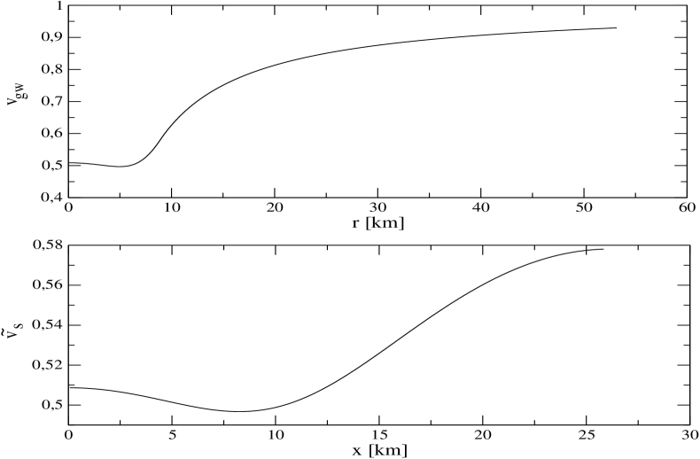
Figure 6.3: Characteristic curve velocity profiles $v_{gw}$ for the master axial equations (3.84) and (4.62), and $\tilde{v}_{s}$ for the radial hyperbolic system of equations (6.30)-(6.31). The radial propagation velocity is plotted in $x$-coordinate. The stellar radius is at $R_{s}=8.862~{}km$ in the $r$-coordinate and is at $R_{s}^{x}=25.80~{}km$ in the $x$-coordinate.

The profile of these velocities for our equilibrium stellar model is plotted in figure 6.3, where the stellar radius is at $R_{s}=8.862~{}km$ in the $r$-grid and is mapped by the tortoise coordinate transformation at $R_{s}^{x}=25.80~{}km$ in the $x$-grid, (see section 6.2). If we define the numerical velocities of the $r$- and $x$-grids respectively as follows:

$$v_{r}=\frac{\Delta r}{\Delta t}\,,\qquad\qquad\qquad v_{x}=\frac{\Delta x}{\Delta\tilde{t}}\,,$$ (6.16)

the CFL condition (6.12) implies that

$$v_{s}<v_{x}\qquad\qquad\qquad v_{gw}<v_{r}\,.$$ (6.17)

Therefore, in order to have the same Eulerian description of the time coordinate in the two grids the following relation between the numerical velocities must be imposed:

$$v_{x}=v_{r}\frac{\Delta r}{\Delta x}\,.$$ (6.18)

We set up in this code the two numerical $r$- and $x$-grids for the interior spacetime, where the $x$-grid dimension is twice the $r$-grid, $J_{x}=2J_{r}$. The coarse dimension for the $r$-grid is $J_{r}=200$, which for the stellar model adopted in this thesis leads to the spatial increment  ${\Delta}r=0.04431~{}km$. This choice leads to an $x$-grid with a dimension $J_{x}=400$ and spatial increment ${\Delta}x=0.0646~{}km$. The CFL condition will certainly be satisfied if we fix the numerical velocity of the  $r$-grid as $v_{r}=0.99$. In fact, the corresponding value for the $x$-grid velocity is $v_{x}=0.67905$, which has been determined from equation (6.18). This value is higher than the physical velocity $\tilde{v}_{s}$ shown in figure 6.3 for the stellar model adopted in this work. The same properties are valid also for higher resolution for the $x$-grid as long as the relation $J_{x}=2J_{r}$ is maintained between the two meshes.

In the exterior spacetime only the $r$-grid is present which conserves the spatial and time steps of the internal mesh.

6.2 Background

The background spacetime is represented by a perfect fluid, spherically symmetric relativistic star in hydrostatic equilibrium. The TOV equations (3.5)-(3.8) and an equation of state, which describes the properties of the stellar matter, form a closed system of equations, which can be integrated by specifying the central density of the star. As explained in section 3.1, in this work we will consider a polytropic equation of state (3.9),

$$p=k\,\rho^{\Gamma}\,.$$ (6.19)

During the numerical integration of the TOV equations, we have found a slight improvement in the rate of convergence by adopting the metric function $\Lambda$ as a new independent variable instead of the mass function $M$. Furthermore, the presence of two numerical meshes in the code requires an integration of the TOV equations in both the $r$- and $x$-grids.

The equilibrium configuration is then the solution of the following system of equations:

$$\widetilde{\mathbf{D}}\Lambda = \left(4\pi r\,\rho\,e^{2\,\Lambda}+\frac{1-e^{2\,\Lambda}}{2r}\right)\,,$$ (6.20)

$$\widetilde{\mathbf{D}}p = -\left(\rho+p\right)\left(4\pi r\,p\,e^{2\,\Lambda}-\frac{1-e^{2\,\Lambda}}{2r}\right)\,,$$ (6.21)

$$\widetilde{\mathbf{D}}\Phi = -\frac{\widetilde{\mathbf{D}}p}{\rho+p}\,,$$ (6.22)

$$\widetilde{\mathbf{D}}r = 1\,,$$ (6.23)

$$p = K\,\rho^{\,\Gamma}\ ,$$ (6.24)

where we have introduce the differential operator $\widetilde{\mathbf{D}}$, which acts on a generic scalar function $f$ as follows:

$$\widetilde{\mathbf{D}}f=\left\{\begin{array}[]{ll}f_{,\,r}&\,\,\textrm{~{}~{}for the}~{}~{}$r$\textrm{\emph{-grid} }\,,\\ \bar{c}_{s}^{\,-1}f_{,\,x}&\,\,\textrm{~{}~{}for the}~{}~{}$x$\textrm{\emph{-grid} }\,.\end{array}\right.$$ (6.25)

This definition allows us to write the same expressions for the TOV equations (6.20)-(6.23) for the “tortoise fluid coordinate” (6.2) as well as for the (area) coordinate $r$. By adopting this new system of equations the mass function $M$ can be determined in terms of the metric function $\Lambda$ with its definition (3.4). In case of an integration carried out in the “fluid tortoise coordinate” frame, the equation (6.23) shows that the radial coordinate $r$ is a scalar field which is an unknown of the system as well as the other metric and fluid variables.

For specific values of the polytropic parameters $K$ and $\Gamma$ in the EOS (6.24), the numerical integration of equations (6.20)-(6.24) can proceed from the stellar origin $r=0$ outward as follows [77]:

• Specification of the central mass-energy density $\rho_{c}$ and consequently the corresponding value of pressure $p_{c}$ determined trough the EOS (6.24).

• Imposition of the boundary conditions at the origin of the coordinates $r=0$ for the metric variables $\Phi$ and $\Lambda$:

  $$\Phi(0)=\Phi_{c}\,,\qquad\qquad\Lambda(0)=0\,.$$ (6.26)

  The second condition in equation (6.26) can be derived from the definition (3.4), and from the behaviour $M\sim O(r^{3})$ given by equation (3.8). On the other hand, the choice of $\Phi_{c}$ is completely arbitrary. Due to the linearity of the ODE (6.22), its value can be later rescaled to the correct one in order to satisfy the matching condition on the stellar surface.

• Integration of the equations (6.20)-(6.24) with a standard numerical method for ODEs [91]. The integration starts from the origin onward and ends when the pressure vanishes $p(r)=0$. This position of null pressure identifies the stellar surface and then the stellar radius $R_{s}$. Thus the value of the mass function in this point $M=M(R_{s})$ is the total gravitational mass of the star.

• Eventually, the function $\Phi$ can be rescaled with a constant value in order to match the Schwarzschild solution on the surface

  $$\Phi(R_{S})=-\Lambda(R_{s})=\frac{1}{2}\ln\left(1-\frac{2M}{R_{s}}\right)\,.$$ (6.27)

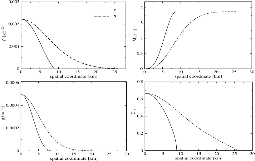
Figure 6.4: For a polytropic non-rotating star with indices $\Gamma=2$, $k=100$ km² and with a central density $\rho_{c}=3\times 10^{15}~{}gcm^{-3}$, we plot the spatial profile of (clockwise from top left): the mass energy density $\rho$, mass function $M$, speed of sound $c_{s}$ and the pressure $p$ respectively. The plots are against the $r$-coordinate (solid line) and $x$-coordinate (dashed line).

We consider a stellar model which is described by the polytropic EOS (6.24) with the following parameters

$$K=100~{}km^{2}\qquad\qquad\Gamma=2\,.$$ (6.28)

This choice allows us to determine a star with a mass and radius similar to those obtained with realistic equation of state of average stiffness. For a supranuclear central density given by $\rho_{c}=3\times 10^{15}~{}gcm^{-3}$, the integration procedure carried out with a fourth order Runge-Kutta (RK4) method [91] provides a star with a radius of $R_{s}=8.862~{}km$ and a mass of $M=1.869~{}km=1.266~{}M_{\odot}$. When we use the $x$-fluid tortoise coordinate, the stellar radius is mapped at $R_{x}=25.840~{}km$. In figure 6.5, one can notice the relation between the $\tilde{r}$ and $x$ representation of the spatial coordinate $r$ and the higher point density near the stellar surface. The equilibrium configuration for all the fluid and metric quantities are plotted in figures (6.4) and (6.5). In the exterior the Schwarzschild solution is described only by the metric functions $\Phi$ and $\Lambda$ that are written in terms of the total gravitational mass of the star as follows:

$$\Phi(r)=-\Lambda(r)=\frac{1}{2}\ln\left(1-\frac{2M}{r}\right)\,,$$ (6.29)

where their values on the stellar surface are given by the junction condition (6.27).

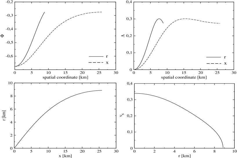
Figure 6.5: For the same stellar model adopted in figure 6.4, the metric quantities $\Phi$ and $\Lambda$ are shown in the two upper plots, where the solutions determined in the $r$-grid are denoted with the solid lines while the dashed lines are relative to the $x$-grid solutions. In the lower figures, the relation between the Schwarzschild $r$-coordinate and the fluid tortoise $x$-coordinate is shown on the left, while the sound velocity $v_{s}$ is on the right.

Finally, we have determined the rate of convergence of the TOV solutions with the method described in appendix G.2 by using three grids of 200,400, and 800 points. The results are shown in table 6.1, where $\sigma_{r}$ and $\sigma_{x}$ are the convergence factor for solutions determined in the $r$- and $x$-coordinates respectively. The fourth order convergence is found in accordance with the numerical scheme used (RK4).

Convergence	m	p	$\rho$	$\bar{c}_{s}$	$\Phi$	$\Lambda$
$\sigma_{x}$	4.017	4.007	4.007	4.007	4.046	4.031
$\sigma_{r}$	4.055	4.000	3.997	3.995	3.987	4.055

Table 6.1: Convergence rate of the TOV solutions for the stellar model considered in this thesis, where $\sigma_{x}$ and $\sigma_{r}$ are calculated for the $x$- and $r$-grids respectively. The convergence factor has been calculated for a set of three grids of dimension (200,400,800). The results confirm the fourth order convergence expected by the accuracy of the RK4 method.

6.3 Linear radial pulsations

The time-evolution of the linear radial pulsations of a static star can be studied with the system of equations (3.30)-(3.34) for the four variables $S^{(1,0)},\eta^{(1,0)},\gamma^{(1,0)},H^{(1,0)}$, which has been presented in section (3.3.1). The presence of hyperbolic and elliptic partial differential equations in this system allows us to choose two integration approaches:

• a purely hyperbolic formulation (PHF), where we solve the three evolution equations (3.30), (3.3.1) and (3.32) and we monitor numerical errors in time by looking at the Hamiltonian constraint (3.34).

• A hyperbolic-elliptic system of equations (HEF), where we integrate Eqs. (3.30) and (3.3.1) and then solve the Hamiltonian constraint (3.34) for the metric variables $S^{(1,0)}$. In this case the constraint will be satisfied by construction.

As shown in figure 6.2, the radial perturbations are first integrated on the $x$-grid. These solutions are then interpolated on the $r$-grid at any time slice. In terms of the fluid tortoise coordinate $x$ defined in equation (6.2) the system of perturbative equations (3.30)-(3.33) becomes the following:

$$\!\!\!\!\!\!\!\!H_{,\,t}^{(1,0)} = -\bar{c}_{s}\,e^{\Phi-\Lambda}\,\gamma^{(1,0)}_{,\,x}-\bar{c}_{s}^{2}\,\left[\left(1-\frac{1}{\bar{c}_{s}^{2}}\right)\left(4\pi\bar{p}\,r+\frac{m}{r^{2}}\right)+\frac{2}{r}\,e^{-2\Lambda}\right.{}$$ (6.30)

$$-\left.4\pi\left(\bar{\rho}+\bar{p}\right)r\,\right]\,e^{\Phi+\Lambda}\,\gamma^{(1,0)}\,,$$

$$\!\!\!\!\!\!\!\!\gamma_{,\,t}^{(1,0)} = -\frac{e^{\Phi-\Lambda}}{\bar{c}_{s}}\,H^{(1,0)}_{,\,x}-4\pi\left(\bar{\rho}+\bar{p}\right)\,r\,e^{\Phi+\Lambda}\,H^{(1,0)}-\left(4\pi\bar{p}\,r^{2}+\frac{1}{2}\right)\,e^{\Phi+\Lambda}S^{(1,0)},$$ (6.31)

$$\!\!\!\!\!\!\!\!S_{,\,t}^{(1,0)} = -8\pi\left(\bar{\rho}+\bar{p}\right)\,e^{\Phi+\Lambda}\,\gamma^{(1,0)}\,,$$ (6.32)

$$\!\!\!\!\!\!\!\!\eta^{(1,0)}_{,\,x} = \bar{c}_{s}\,4\pi(\bar{\rho}+\bar{p})\,r\,\left[r\,S^{(1,0)}+\left(1+\frac{1}{\bar{c}^{2}_{s}}\right)H^{(1,0)}\right]\,e^{2\Lambda}\,,$$ (6.33)

and the Hamiltonian constraint (3.34) is given by:

$$S^{(1,0)}_{,\,x}=\bar{c}_{s}\left(8\pi\bar{\rho}r-\frac{2}{r}+\frac{2m}{r^{2}}\right)e^{2\Lambda}\,S^{(1,0)}+8\pi\frac{\bar{\rho}+\bar{p}}{\bar{c}_{s}}\,e^{2\Lambda}\,H^{(1,0)}\,.$$ (6.34)

6.3.1 Numerical algorithm

The two evolution equations (6.30) and (6.31) for the enthalpy $H^{(1,0)}$ and the radial velocity $\gamma^{(1,0)}$ perturbations can be solved with various PDE numerical algorithms [91]. We have used a two-step McCormack algorithm (see appendix G), which implements a predictor and corrector step and provides second order approximation in space and time. For the predictor step the finite difference approximation of equations (3.30) and (3.3.1) reads:

$$\widetilde{H}_{j}^{n+1} = H_{j}^{n}-e^{\Phi_{j}-\Lambda_{j}}\,(\bar{c}_{s})_{\,j}\,\frac{{\Delta}t}{{\Delta}x}\,\left(\gamma_{j}^{n}-\gamma_{j-1}^{n}\right)+{\Delta}t\,(b_{1})_{j}\,\frac{\gamma_{j-1}^{n}+\gamma_{j}^{n}}{2}\,,$$ (6.35)

$$\widetilde{\gamma}_{j}^{n+1} = \gamma_{j}^{n}-e^{\Phi_{j}-\Lambda_{j}}\,\frac{{\Delta}t}{{\Delta}x}\,\frac{H_{j}^{n}-H_{j-1}^{n}}{(\bar{c}_{s})_{j}}+{\Delta}t\,(b_{2})_{j}\,\frac{H_{j-1}^{n}+H_{j}^{n}}{2}$$ (6.36)

$$+{\Delta}t\,(b_{3})_{j}\,\frac{S_{j-1}^{n}+S_{j}^{n}}{2}\,.$$

The values found, which have been denoted with a tilde, are now used in the corrector step as follows:

$$H_{j}^{n+1} = H_{j}^{n}-e^{\Phi_{j}-\Lambda_{j}}\,(\bar{c}_{s})_{j}\,\frac{{\Delta}t}{{\Delta}x}\,\frac{\gamma_{j}^{n}-\gamma_{j-1}^{n}+\widetilde{\gamma}_{j+1}^{n+1}-\widetilde{\gamma}_{j}^{n+1}}{2}$$ (6.37)

$$+{\Delta}t\,(b_{1})_{j}\,\frac{\gamma_{j}^{n}+\gamma_{j-1}^{n}+\widetilde{\gamma}_{j+1}^{n+1}+\widetilde{\gamma}_{j}^{n+1}}{4}\,,$$

$$\gamma_{j}^{n+1} = \gamma_{j}^{n}-\frac{e^{\Phi_{j}-\Lambda_{j}}}{(\bar{c}_{s})_{j}}\,\frac{{\Delta}t}{{\Delta}x}\,\frac{H_{j}^{n}-H_{j-1}^{n}+\widetilde{H}_{j+1}^{n}-\widetilde{H}_{j}^{n}}{2}$$ (6.39)

$$+{\Delta}t\,(b_{2})_{j}\,\frac{H_{j}^{n}+H_{j-1}^{n}+\widetilde{H}_{j+1}^{n+1}+\widetilde{H}_{j}^{n+1}}{4}$$

$$+{\Delta}t\,(b_{3})_{j}\,\frac{S_{j}^{n}+S_{j-1}^{n}+\widetilde{S}_{j+1}^{n+1}+\widetilde{S}_{j}^{n+1}}{4}\,.$$

The coefficients $(b_{1})_{j},(b_{2})_{j}$ and $(b_{3})_{j}$ are the discrete approximations in $r_{j}$ of the following background quantities:

$$b_{1} = -\bar{c}_{s}^{2}\,\left[\left(1-\frac{1}{\bar{c}_{s}^{2}}\right)\left(4\pi\bar{p}\,r+\frac{m}{r^{2}}\right)+\frac{2}{r}\,e^{-2\Lambda}-4\pi\left(\bar{\rho}+\bar{p}\right)\right]\,e^{\Phi+\Lambda}\,,$$ (6.40)

$$b_{2} = -4\pi\left(\bar{\rho}+\bar{p}\right)\,r\,e^{\Phi+\Lambda}\,,$$ (6.41)

$$b_{3} = -\left(4\pi\bar{p}\,r^{2}+\frac{1}{2}\right)\,e^{\Phi+\Lambda}\,.$$ (6.42)

The metric variable $S^{(1,0)}$ can be updated at every time–step with one of the two equations (6.32) and (6.34). In a purely hyperbolic formulation (PHF) the variable is evolved by the equation (6.32), which can be solved with an up–wind method [91] where we have introduced a second order approximation in space. The numerical algorithm is then given by

$$S^{n+1}_{j}=S^{n}_{j}+{\Delta}t\,(b_{4})_{j}\,\frac{\gamma^{n}_{j}+\gamma^{n}_{j+1}}{2}\,,$$ (6.43)

where the coefficient $b_{4}$ is

$$b_{4}=-8\pi\left(\bar{\rho}+\bar{p}\right)\,e^{\Phi+\Lambda}\,.$$ (6.44)

Alternatively, in the hyperbolic–elliptic formulation (HEF) discussed above we can integrate the Hamiltonian constraint (6.34) as an ODE at any time step. The equation (6.34) can be discretized by using a second order finite approximations in space and then written as a tridiagonal linear system. We can then use a standard $\mathbf{LU}$ decomposition and a “tridiagonal subroutine” [91] for getting the value of $S^{(1,0)}$. The components of the $\mathbf{LU}$ decomposition of equation (6.34) are given by the following expressions:

$$a_{j}S_{j-1}^{n}+b_{j}S_{j}^{n}+c_{j}S_{j+1}^{n}=f_{j}\,$$ (6.45)

where the coefficients $a,b,c$, and $f$ are

$$a = -\frac{e^{-2\Lambda}}{2}\frac{1}{{\Delta}x}\,,$$ (6.46)

$$b = -\bar{c}_{s}\left(8\pi\bar{\rho}r-\frac{2}{r}+\frac{2m}{r^{2}}\right)e^{2\Lambda}\,,$$ (6.47)

$$c = \frac{e^{-2\Lambda}}{2}\frac{1}{{\Delta}x}\,,$$ (6.48)

$$f = 8\pi\frac{\bar{\rho}+\bar{p}}{c_{s}}\,H^{(1,0)}\,.$$ (6.49)

The other metric perturbation $\eta^{(1,0)}$ can be solved by integrating equation (6.33). At any time slice, this equation is a two point boundary value problem that must satisfy the condition (3.39) at the origin and vanishes on the surface. We use a shooting method, where the integration is carried out from the origin to the surface by specifying an initial guess for $\eta^{(1,0)}$ at origin. The algorithm will shoot the solution up to the surface and control whether the surface condition is satisfied. If not, the routine will correct the value of the variable at the origin and repeats the operation until the surface condition is fulfilled.

6.3.2 Boundary conditions

The condition at the origin for the radial perturbations are given by equations (3.38)-(3.41). We implement a grid where the first point of the spatial coordinate $r_{1}$ is not at the origin $r_{0}=0$ but at $r_{1}=r_{0}+{\Delta}r$, where ${\Delta}r$ is the spatial grid step. The boundary condition at the origin of the perturbative variables is then implemented at $r_{1}$ by using the behaviours (3.38)-(3.41), which have been obtained with a Taylor expansion. This procedure is particularly useful in the axial sector [95] for avoiding numerical instability which can be generated by the presence of the term $l(l+1)r^{-2}$ in the potential of the axial master equation [95]. This method for the radial quantities $\gamma^{(1,0)}$ and $S^{(1,0)}$ gives

$$\gamma_{1}^{n}=\frac{r_{1}}{r_{2}}\,\gamma_{2}^{n}\,,\qquad\qquad\qquad S_{1}^{n}=\frac{r_{1}}{r_{2}}\,S_{2}^{n}\,,$$ (6.50)

where we have assumed that the behaviours (3.38)-(3.41) are valid for both the first and second grid points $r_{1}$ and $r_{2}$. For the enthalpy $H^{(1,0)}$ and the other metric perturbation $\eta^{(1,0)}$ we implemented the following conditions:

$$H_{1}^{n}=\frac{4H_{2}^{n}-H_{3}^{n}}{3}\,,\qquad\qquad\qquad\eta_{1}^{n}=\frac{4\eta_{2}^{n}-\eta_{3}^{n}}{3}\,,$$ (6.51)

which have been determined by spatial differentiation of equations (3.40) and (3.39), and using the second order finite one-sided approximation (F.7) for the first order derivative. This condition for $\eta^{(1,0)}$ can be also derived by the constraint (6.33).

At the surface the vanishing of the Lagrangian perturbation of the pressure leads to equation (3.48) for the variable $\gamma^{(1,0)}$. The stellar matter in our model is described by a polytropic EOS, where pressure, mass energy density and speed of sound vanish on the surface. Therefore, the condition (3.48) is certainly satisfied if the velocity $\gamma^{(1,0)}$ and its spatial derivative $\gamma^{(1,0)}_{,\,r}$ are finite. According to the fluid tortoise transformation (6.3) the spatial derivative in the tortoise coordinate is related to the derivative in $r$ by the following expression:

$$\gamma^{(1,0)}_{,\,x}=\bar{c}_{s}\gamma^{(1,0)}_{,\,r}\,.$$ (6.52)

Hence, on the stellar surface we can impose the vanishing of $\gamma^{(1,0)}_{,\,x}$ which also ensures the finiteness of $\gamma^{(1,0)}$ and $\gamma^{(1,0)}_{,\,r}$ [95]. The second order finite one-sided approximation (F.8) of the first order spatial derivative leads to the following expression:

$$\gamma_{J_{x}}^{n}=\frac{4\gamma_{Jx-1}^{n}-\gamma_{J_{x}-2}^{n}}{3}\,.$$ (6.53)

The other values for the enthalpy and the metric variable $S^{(1,0)}$ can be directly determined by the perturbative equations (6.30) and (6.34), while for $\eta^{(1,0)}$ we can easily implement its trivial condition, i.e. $\eta^{(1,0)}=0$. The resulting expressions are the following:

$$S_{J_{x}}^{n} = \frac{4S_{J_{x}-1}^{n}-S_{J_{x}-2}^{n}}{3}\,,$$ (6.54)

$$H_{J_{x}}^{n} = H_{J_{x}}^{n-1}+{\Delta}t\,(b_{5})_{J_{x}}\gamma^{n}_{J_{s}}\,,$$ (6.55)

$$\eta_{J_{s}}^{n} = 0\,.$$ (6.56)

where we have used the finite difference approximation (F.8) also for the condition (6.54). The coefficient $b_{5}$ is so defined:

$$b_{5}=-\left(4\pi\bar{p}r+\frac{m}{r^{2}}\right)e^{\Phi+\Lambda}\,.$$ (6.57)

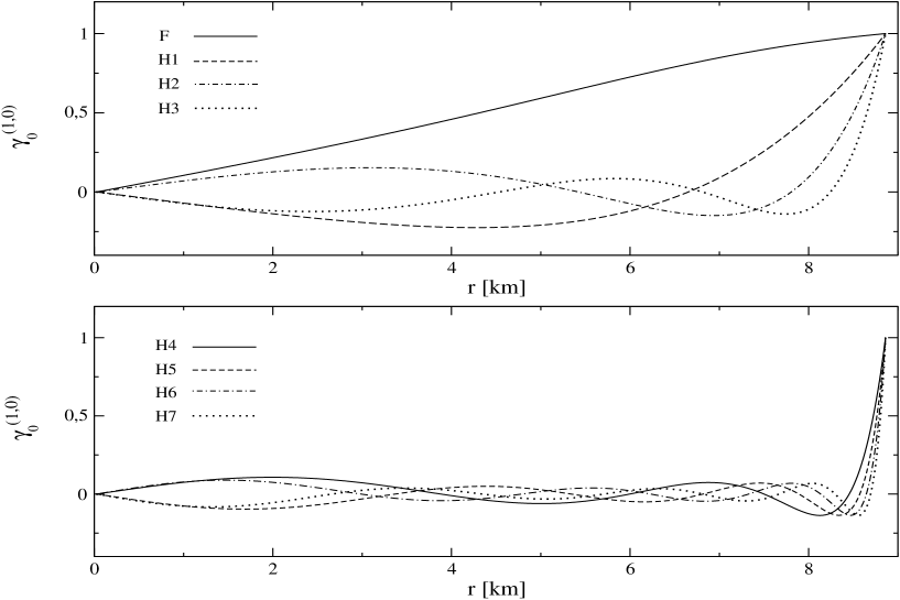
Figure 6.6: Eigenfunctions of the radial perturbation $\gamma^{(1,0)}$. The upper panel displays the eigenfunctions of the fundamental mode and the first three overtones, while the lower panel from the fourth to the seventh overtones.

6.3.3 Initial configuration for radial pulsations

The time–domain integration of the radial perturbative equations (6.30)-(6.33) requires the choice of initial values for the variables $\gamma^{(0,1)}$, $H^{(0,1)}$, $S^{(0,1)}$ and $\eta^{(0,1)}$ on a Cauchy surface. However, the presence of two constraint equations implies that we can independently specify two perturbations. In addition, the radial perturbations must satisfy the boundary conditions on the initial slice as well as along the time evolution. These conditions are certainly satisfied if we specify a profile only for the radial velocity perturbation $\gamma^{(1,0)}$ and set to zero the enthalpy perturbation $H^{(0,1)}$, as the constraint equations (6.33) and (6.34) and boundary conditions imply the vanishing also of the two metric perturbations $S^{(0,1)}$ and $\eta^{(0,1)}$. In the case of a single eigenfunction, this corresponds to a choice of the origin of time. Indeed, as we can see from the radial perturbative equations (6.30)-(6.33), we can consistently choose a normal mode oscillation with eigenfunction $\omega_{n}$ to have the form:

$$\gamma^{(1,0)} = \gamma^{(1,0)}_{n}(r)\cos\omega_{n}t\,,\qquad\qquad H^{(1,0)}=H^{(1,0)}_{n}(r)\sin\omega_{n}t\,,$$

$$S^{(1,0)} = S^{(1,0)}_{n}(r)\sin\omega_{n}t\,,\,\,\,\qquad\qquad\eta^{(1,0)}=\eta^{(1,0)}_{n}(r)\sin\omega_{n}t\,,$$

thus at $t=0$ only $\gamma^{(1,0)}$ is nonvanishing. With this choice the Hamiltonian constraint (6.34) is initially satisfied by construction. This choice is also consistent in the case of an initial Gaussian pulse, which can be considered as a particular linear conbination of the eigenmodes (LABEL:Rad_Ic).

The time evolution of radial pulsations of a spherically symmetric perfect fluid star is completely determined by a complete set of radial eigenfunctions. In this work, we consider two different configurations for the dynamical evolution, respectively described by: i) the presence of a broad range of normal mode frequencies, ii) the excitation of a few selected radial modes. The first configuration can be accomplished by imposing for $\gamma^{(1,0)}$ an initial Gaussian pulse so that many radial modes are excited at the same time. This kind of initial data is mainly used to test and calibrate the reliability of the code. On the other hand, the second configuration can be determined by imposing as initial data the eigenfunctions of $\gamma^{(1,0)}$ in order to excite the desired associated eigenfrequencies.
The eigenvalue problem for the radial perturbation $\gamma^{(1,0)}$ has been described in section 3.3.3. However, since the simulations for the radial perturbations are carried out on the $x$-grid we have to introduce the tortoise fluid coordinate also in the Sturm-Liouville problem (3.57). The system of two ordinary differential equations (3.58)-(3.59) transforms as follows:

$$y_{,x}^{(1,0)} = \bar{c}_{s}\frac{z}{\hat{P}}^{(1,0)}\,,$$ (6.59)

$$z_{,x}^{(1,0)} = -\bar{c}_{s}\left(\omega^{2}\hat{W}+\hat{Q}\right)y^{(1,0)}\,,$$ (6.60)

and the functions $\hat{W},\hat{P},\hat{Q}$ are given by:

$$r^{2}\hat{W} \equiv \left(\bar{\rho}+\bar{p}\right)\,e^{3\Lambda+\Phi},$$ (6.61)

$$r^{2}\hat{P} \equiv \left(\bar{\rho}+\bar{p}\right)\,\bar{c}_{s}^{2}\,\bar{p}\,e^{\Lambda+3\Phi}\,,$$ (6.62)

$$r^{2}\hat{Q} \equiv \left(\bar{\rho}+\bar{p}\right)\,\left[\frac{1}{\bar{c}_{s}^{2}}\Phi_{,x}^{2}-\frac{4}{r\bar{c}_{s}}\,\Phi_{,x}-8\pi\,\bar{p}\,e^{2\Lambda}\right]\,e^{\Lambda+3\Phi}\,.$$ (6.63)

Now, the boundary conditions at the origin and surface are:

$$y_{0}=\bar{c}_{s}\frac{z_{0}}{3P}\,,\qquad\qquad\qquad\left.(\bar{\rho}+\bar{p})\,\bar{c}_{s}\,e^{-\Phi}y^{(1,0)}_{,x}\right|_{r=R_{x}}=0\,.$$ (6.64)

The method used to integrate the radial eigenvalue system of equations (6.59)-(6.60) is the “relaxation method” [91]. The first eight eigenfunctions for the radial velocity $\gamma^{(1,0)}$ are plotted in figure 6.6 with respect to the $r$ coordinate and after a normalization with the norm of their maximum value. These profiles have the characteristic node numbers expected by the theory, i.e. absence of nodes for the F-mode, and a node number equal to the order of the overtone. The associated eigenfrequencies are written in table 6.2. The first three have been compared with published values obtained by Kokkotas and Ruoff [59] for our stellar model. The results are accurate to better than $0.2$ percent (see table 6.2). The rate of convergence for the eigenfrequencies and eigenfunctions is of second order, as expected by the accuracy of the numerical method.

Normal mode	Frequecy domain	Time domain	Kokkotas and Ruoff	Relative error
	[kHz]	[kHz]	[kHz]
F	2.138	2.145	2.141	0.10 %
H1	6.862	6.867	6.871	0.13 %
H2	10.302	10.299	10.319	0.16 %
H3	13.545	13.590		0.33 %
H4	16.706	16.737		0.18 %
H5	19.823	19.813		0.05 %
H6	22.914	22.889		0.11 %
H7	25.986	25.964		0.08 %

Table 6.2: The table shows the eigenfrequencies of the first eight normal modes of the radial perturbations, which have been determined with the Sturm-Liouville problem (second column) and with an FFT of the time evolution (third column). The first three normal modes obtained in frequency domain have been compared with those published by Kokkotas and Ruoff [59] (fourth column), and the relative error is given in the first three rows of the last column. The remaining rows display the relative errors between the frequency determined in the time and frequency domains.

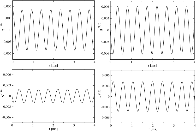
Figure 6.7: Time evolution of the four radial perturbations, where the oscillations have been excited with the F-mode eigenfunction of the variable $\gamma^{(1,0)}$. The quantities have been averaged in the interior spacetime by using the definition (6.66).

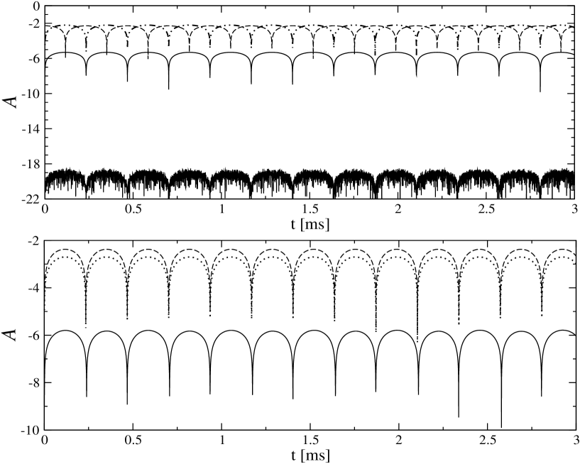
Figure 6.8: The fundamental mode oscillations of the four radial perturbations are compared with the numerical errors due to the violation of the Hamiltonian constraint. The quantities are plotted in semilogarithmic scale after having performed the spatial average as defined in equation (6.66). In the upper and lower panels are shown the results for a HEF and PHF formulation respectively. In both figures the curves relative to the Hamiltonian constraints are represented in (solid lines) while the radial perturbations in dashed and point-dashed line. For the details of the results, see the discussion in section 6.3.4.

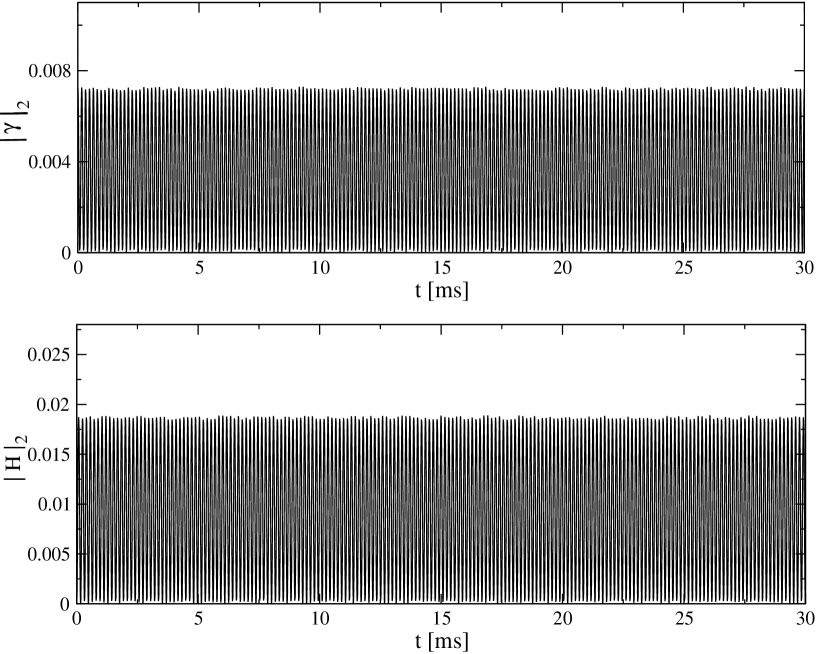
Figure 6.9: Norms of the radial perturbations $\gamma^{(1,0)}$ and $H^{(1,0)}$ for a $30~{}ms$ simulation where only the F-mode has been excited.

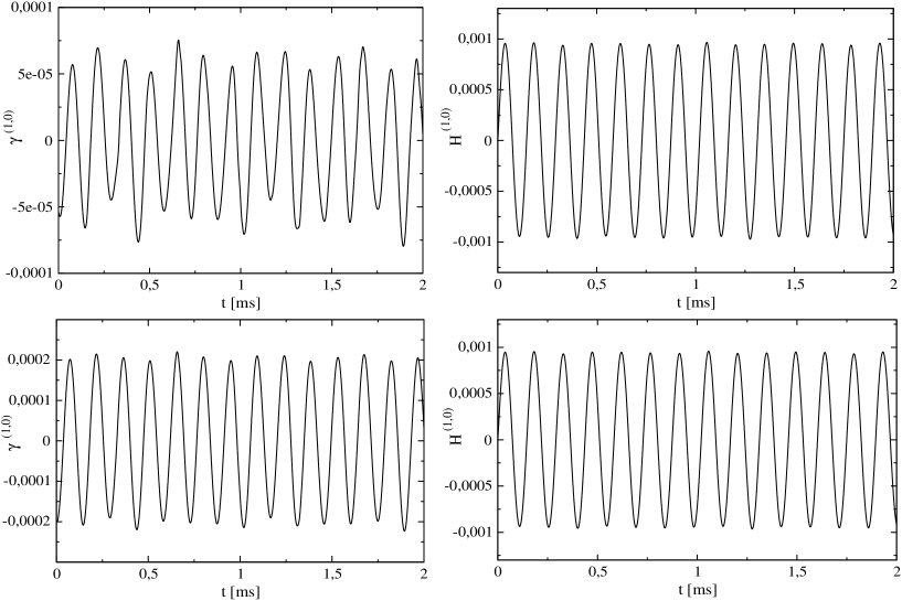
Figure 6.10: Time evolution of the spatial average (6.66) for the radial variables $\gamma^{(1,0)}$ and $H^{(1,0)}$. The pulsations have been excited with the eigenfunction of $\gamma^{(1,0)}$ associated with the first overtone. On the top, the averages have been calculated in the whole interior spacetime. On the bottom, the three grid points near the surface have been neglected.

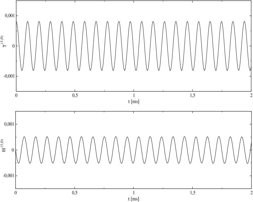
Figure 6.11: Time evolution of the spatial average profiles of the radial variables $\gamma^{(1,0)}$ and $H^{(1,0)}$. The radial pulsations have been excited with the eigenfunction of $\gamma^{(1,0)}$ associated with the second overtone.

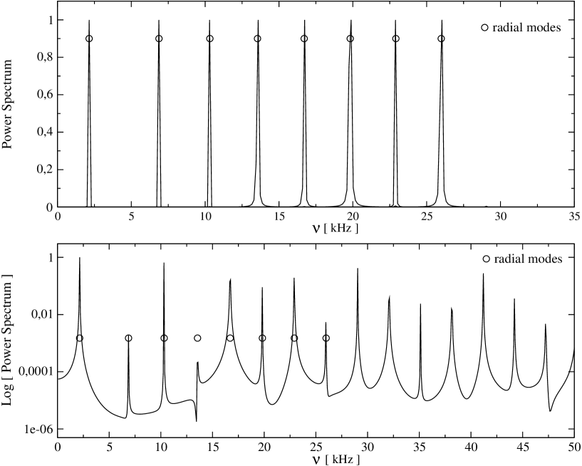
Figure 6.12: Power spectrum of the radial perturbation $\gamma^{(1,0)}$, which has been determined by an FFT of the time profiles. In the upper panel we show in the same plot the spectrum of eight different time evolutions, where everytime a single radial mode has been excited. In the lower panel,we show the spectrum of a time evolution excited by an initial Gaussian pulse. The excitation of the radial modes is evident in both cases. The first eight frequencies are compared to the values determined with a code in the frequency domain and are shown with a circle.

6.3.4 Simulations of radial perturbations

The analysis of the radial oscillation part of the code starts with a pulsating configuration described by selected radial modes. The desired oscillation frequency is excited by introducing the initial condition (LABEL:Rad_Ic), where at $t=0$ the eigenfunction of the velocity perturbation $\gamma^{(1,0)}$ is given by

$$\gamma^{(1,0)}_{in}=A^{(1,0)}\gamma^{(1,0)}_{n}$$ (6.65)

where we have introduced a constant factor $A^{(1,0)}$ to control the amplitude of the oscillations and $\gamma^{(1,0)}_{n}$ is one of the normalized eigenfunctions plotted in figure 6.6. The first simulation is carried out for the fundamental mode with an initial amplitude of $A^{(1,0)}=0.01$ and for an evolution time of $4~{}ms$. The $x$-grid has dimension $J_{x}=400$, while the time step is chosen as explained in section 6.1.2 in order to satisfy the CFL condition and have the same Eulerian time discrete representation of the $r$-grid. The evolution of the four radial perturbations $\gamma^{(1,0)},~{}H^{(1,0)},~{}S^{(1,0)}$ and $\eta^{(1,0)}$ is shown in figure 6.7, where we have plotted the following average values determined at any time step:

$$<f>=\frac{1}{R_{s}}\int_{0}^{R_{s}}fdr\,,$$ (6.66)

in order to have global information about the oscillation properties of the variables studied. The function $f$ in equation (6.66) obviously represents one of the four radial perturbations cited above. The results show the typical periodic character of the adiabatic radial pulsations. This monochromatic character is also confirmed by their spectra (figure 6.12) which have been determined with a Fast Fourier Transformation (FFT) of the simulations.

In order to test the stability and possible numerical dissipative effects, we perform a longer simulation of $30~{}ms$ and we monitor the Hamiltonian constraint and determine the $L_{2}$ norms of the variables under consideration. In figure 6.8, we show the oscillation amplitude on a logarithmic scale of the four radial perturbations, i.e $\gamma^{(1,0)},H^{(1,0)},S^{(1,0)},\eta^{(1,0)}$, and the numerical errors due to the violation of the Hamiltonian constraint for a hyperbolic-elliptic formulation (HEF) (upper panel) and a purely hyperbolic formulation (PHF) (lower panel). In the HEF, the Hamiltonian constraint (solid lines) remained bounded and is three orders of magnitude lower than the amplitude of the radial perturbations $\gamma^{(1,0)}$ and $H^{(1,0)}$, which are denoted with a dashed and point-dashed line respectively. In addition, when we perform the average (6.66) of the Hamiltonian constraint by neglecting the first two grid points $r_{1}$ and $r_{2}$, we find an appreciable reduction of the numerical errors. As shown by the lowest solid line the numerical errors are less than $10^{-18}$. This accuracy is expected as the Hamiltonian constraint in the HEF is solved by updating one of the radial variables. However, the results show that the implementation of boundary conditions at the centre of the star introduce some numerical errors which is anyway three orders of magnitude lower than the radial physical oscillations and is not propagated along the star. We perform a similar analysis for the PHF (lower panel of figure 6.8) by comparing the two metric radial perturbations $S^{(1,0)}$ and $\eta^{(1,0)}$ (dashed and point-dashed line respectively) with the numerical oscillations due to the violations of the Hamiltonian constraints (solid line). We can conclude that even for this case the constraint is well satisfied.

The stability of the radial simulations is confirmed also by the analysis of the $L_{2}$ norms. For a $30~{}ms$ evolution excited by the eigenfunction of $\gamma^{(1,0)}$ associated with the F-mode, the $L_{2}$-norms for $\gamma^{(1,0)}$ and $H^{(1,0)}$ show a constant oscillatory character without any presence of dissipative effects (see figure 6.9). The properties of the Hamiltonian constraint violation and $L_{2}$-norms illustrated for the case of an evolution dominated by the F-mode, remains valid also when the other overtones are excited and the simulations preserve their stability and absence of dissipation also for longer evolutions.

The simulations carried out with the excitation of the first overtone (H1) show a behaviour near the surface that deserves some attention. In figure 6.10, we plot the time profile of the two fluid radial perturbations $\gamma^{(1,0)}$ and $H^{(1,0)}$. The two upper panels have been obtained by performing the average (6.66) for the interior spacetime, while on the bottom the last three grid points that are near the surface have been neglected from the average operation. We can first notice that the enthalpy $H^{(1,0)}$ preserves the same oscillating properties while the velocity $\gamma^{(1,0)}$ has a higher amplitude and a smoother oscillating dynamics when the points near the surface are neglected. By investigating the movie of these simulations for the variable $\gamma^{(1,0)}$, we have noticed the presence of small spurious oscillations near the surface. This numerical noise is not continuous but has a random character, which is sufficient to modify the evolution of this variable. In order to have a better understanding we have also analyzed the simulations for the second (H2) and third overtones (H3). Similarly to the case of the F-mode, the spatial average profiles of these time evolutions do not present any spurious oscillations near the surface. For the second overtone, this behaviour is shown in figure 6.11. However, when we study the corresponding movies we notice also in these cases the presence of random and very small spurious oscillations near the surface that decrease by increasing the resolution of the meshes. From the analysis of the movies and the eigenfunction profiles, we can argue that for the H2 and H3 normal modes the presence of a node near the surface seems to prevent the propagation of these oscillations along the star and actually reduce their effects. On the other hand for the F-mode, the absence of micro-oscillations in the time profiles of figure 6.7 seems more due to the smallness of these numerical oscillations with respect to the average value of the physical pulsations, about two order of magnitude less. This motivation is confirmed by the analysis of the non-linear simulations when the F-mode will display this noise. As a result, the presence of these oscillations has to be taken into account during the implementation of the matching conditions of the non-linear perturbations.

The spectral properties of the oscillations are studied by performing an FFT of the time profiles. In figure 6.12 we show the power spectrum of seven simulations where every time only one of the first seven normal modes has been excited by the initial configuration. Furthermore, we have performed a $12~{}ms$ simulation for radial pulsations excited by an initial Gaussian pulse. The relative spectrum is shown in the lower panel of figure 6.12, where the frequencies of the normal modes are labelled with a circle. The radial modes are determined in time domain with an accuracy to better than $0.3\%$, see table 6.2.

Eventually, we determine the convergence rate for the radial evolution which is given in table 6.3 for the four radial perturbations.

Convergence	$~{}\gamma^{(1,0)}~{}$	$~{}H^{(1,0)}~{}$	$~{}S^{(1,0)}~{}$	$~{}\eta^{(1,0)}~{}$
$\sigma^{(1,0)}$	2.04	2.06	2.07	1.53

Table 6.3: Convergence test for radial perturbations: $\sigma^{(1,0)}$ denotes the convergence rate in the $L_{2}$ norm.

The amount of pulsation energy contained in the radial perturbations can be determined with the expressions of the relativistic kinetic and potential energy derived with a variational analysis [22, 23, 76], and [17]. In particular, according to the initial conditions that we have set up for the radial perturbations we can derive the pulsation energy introduced on the initial Cauchy surface. For an initial vanishing Lagrangian displacement and a specific eigenfunction for the radial velocity $\gamma^{(1,0)}$, the initial pulsation energy is given by the kinetic energy [17]:

$$E^{(1,0)}_{n}=2\pi W\left(A^{(1,0)}\right)^{2}\int_{0}^{R_{s}}dr\left(r^{2}e^{-\Lambda}\gamma^{(1,0)}_{n}\right)^{2}\,,$$ (6.67)

where we have used the relation (3.55), and $\gamma^{(1,0)}_{n}$ is an eigenfunction of $\gamma^{(1,0)}$ and $A^{(1,0)}$ its amplitude. In table 6.4, the oscillation energy for the first seven normal modes has been calculated with the expression (6.67) for an amplitude $A^{(1,0)}=0.001$.

6.4 Linear, axial non-radial oscillations

The dynamics of axial perturbations on a static star is described by the system of two differential equations: the odd-parity master equation (3.84) for the axial master variable $\Psi^{(0,1)}$ and the conservation equation (3.85), which is satisfied by the redefined axial velocity perturbation $\hat{\beta}^{(0,1)}$. In section (3.5) we have already shown that the functional form of the conservation equation  (3.85) allows us to discern the dynamical degree of freedom of the axial gravitational spacetime from the stationary frame dragging profile produced by the presence of an axial differential rotation. Hence, the solution of the master equation (3.84) can be decomposed in two parts (3.87),

$$\Psi^{(0,1)}=\Psi^{(0,1)}_{hom}+\Psi^{(0,1)}_{p}\,,$$ (6.68)

namely the solution $\Psi^{(0,1)}_{hom}$ of the homogeneous equation (3.88) plus a particular static solution $\Psi^{(0,1)}_{p}$ of equation (3.89).

6.4.1 Numerical algorithm

The homogeneous equation (3.88) is integrated by means of a standard leapfrog method, which is an explicit second order and three level method [91]. By using a centred finite differential approximation in space and time we can write the discrete approximation of equation (3.88) as follows:

$$-\frac{\psi^{n+1}_{j}-2\psi^{n}_{j}+\psi^{n-1}_{j}}{{\Delta}t^{2}}+v^{2}_{j}\,\frac{\psi^{n}_{j+1}-2\psi^{n}_{j}+\psi^{n}_{j-1}}{{\Delta}r^{2}}+\alpha_{j}\,\frac{\psi^{n}_{j+1}-\psi^{n}_{j-1}}{2{\Delta}r}+V_{j}\,\psi^{n}_{j}=0\,.$$ (6.69)

Thus, the value of $\psi_{hom}^{(0,1)}$ is updated in time with the following expression:

$$\psi^{n+1}_{j} = 2\psi^{n}_{j}-\psi^{n-1}_{j}+\frac{{\Delta}t^{2}}{{\Delta}r^{2}}v^{2}_{j}\,\left(\psi^{n}_{j+1}-2\psi^{n}_{j}+\psi^{n}_{j-1}\right)+\alpha_{j}\,{\Delta}t^{2}\,\frac{\psi^{n}_{j+1}-\psi^{n}_{j-1}}{2{\Delta}r}+V_{j}\,{\Delta}t^{2}\,\psi^{n}_{j}\,.$$

The coefficient $v$ is the propagation speed of the wave and $\alpha,V$ are coefficients depending only on the coordinate $r$:

$$v = e^{\Phi-\Lambda}\,,$$ (6.71)

$$\alpha = e^{2\Phi}\left(\frac{2M}{r^{2}}-4\pi\left(\bar{\rho}-\bar{p}\right)r\right)\,,$$ (6.72)

$$V = e^{2\Phi}\left(\frac{6M}{r^{3}}-4\pi\left(\bar{\rho}-\bar{p}\right)-\frac{l(l+1)}{r^{2}}\right)\,.$$ (6.73)

The particular solution is obtained from equation (3.89), which is second-order discretized in space and written as a tridiagonal linear system, which is then solved using a standard $\mathbf{LU}$ decomposition [91]. The components of the $\mathbf{LU}$ decomposition are given by

$$\hat{a}_{j}\psi_{j-1}^{n}+\hat{b}_{j}\psi_{j}^{n}+\hat{c}_{j}\psi_{j+1}^{n}=\hat{f}_{j}$$ (6.74)

where the coefficients $\hat{a}_{j},\hat{b}_{j}$, and $\hat{c}_{j}$ are

$$\hat{a} = \frac{1}{{\Delta}r^{2}}-\left(\frac{2m}{r^{2}}-4\pi\left(\bar{\rho}-\bar{p}\right)r\right)\frac{e^{2\Lambda}}{2{\Delta}r}\,,$$ (6.75)

$$\hat{b} = Ve^{-2\Phi}-\frac{2}{{\Delta}r^{2}}\,,$$ (6.76)

$$\hat{c} = \frac{1}{{\Delta}r^{2}}+\left(\frac{2m}{r^{2}}-4\pi\left(\bar{\rho}-\bar{p}\right)r\right)\frac{e^{2\Lambda}}{{\Delta}r}\,,$$ (6.77)

$$\hat{f} = 16\pi\left(4\pi pr^{2}+\frac{m}{r}\right)e^{3\Lambda}\hat{\beta}^{(0,1)}+16\pi re^{\Lambda}\hat{\beta}^{(0,1)}_{,\,r}\,.$$ (6.78)

The dragging of the inertial frame can be determined by using expression (3.91) and the relation (2.110), which connects the particular solution $\Psi^{(0,1)}_{p}$ with the metric perturbation components $k_{0}^{lm}$ and $h_{0}^{lm}$. Alternatively, the metric variable $k_{0}^{lm}$ as well as the related frame dragging $\omega^{lm}$ can also be determined directly by the ordinary differential equation (3.92). We can apply the same procedure used for solving the particular solution $\Psi^{(0,1)}_{p}$. In this case the $\mathbf{LU}$ decomposition reads:

$$\tilde{a}_{j}k_{0,\,j-1}^{n}+\tilde{b}_{j}k_{0,\,j}^{n}+\tilde{c}_{j}k_{0,\,j+1}^{n}=\tilde{f}_{j}$$ (6.79)

where the coefficients $\tilde{a}_{j},\tilde{b}_{j}$, and $\tilde{c}_{j}$ are

$$\tilde{a} = \frac{e^{-2\Lambda}}{{\Delta}r^{2}}+\frac{2\pi r}{{\Delta}r}\left(\bar{\rho}+\bar{p}\right)\,,$$ (6.80)

$$\tilde{b} = 8\pi\left(\bar{\rho}+\bar{p}\right)-\frac{l(l+1)}{r^{2}}+\frac{4m}{r^{3}}-\frac{2e^{-2\Lambda}}{{\Delta}r^{2}}\,,$$ (6.81)

$$\tilde{c} = \frac{e^{-2\Lambda}}{{\Delta}r^{2}}-\frac{2\pi r}{{\Delta}r}\left(\bar{\rho}+\bar{p}\right)\,,$$ (6.82)

$$\tilde{f} = 16\pi e^{\Phi}\hat{\beta}^{(0,1)}\,.$$ (6.83)

6.4.2 Boundary conditions and initial configuration

The boundary conditions at the origin, stellar surface and at infinity are implemented in accordance with the discussion given in section 3.5. At the origin we impose the condition (3.95) at the first grid point $r_{1}=\Delta r$ as follows:

$$\Psi^{(0,1)}_{1}=\Psi^{(0,1)}_{2}\,\left(\frac{r_{1}}{r_{2}}\right)^{l+1}\,.$$ (6.84)

At infinity we use a standard outgoing wave condition. We carry out the integration of the wave equation (3.88) for the homogeneous solution and the ordinary equation (3.89) for the particular solutions on the whole numerical grid without imposing any condition at the stellar surface. We have found that the numerical solutions satisfy the continuity of the function $\psi^{(0,1)}$ and its first spatial derivatives $\psi^{(0,1)}$, which are the requirements prescribed by the junction conditions. For the two point boundary value problems (3.89) and (3.92), we have imposed at the centre and at infinity the conditions discussed in section 3.5.

The system of equations (3.84) and (3.85) requires the specification of three functions on the initial Cauchy surface, namely

$${\cal I}^{(0,1)}=\left(\Psi^{(0,1)},\Psi_{,\,t}^{(0,1)},\beta^{(0,1)}\right)\ .$$ (6.85)

In the initial data we specify the original axial perturbations $\beta^{(0,1)}$ and we determine the function $\hat{\beta}^{(0,1)}$ according to equation (3.86).

We can set up two independent classes of initial conditions for the first–order fields:

• a stationary differentially rotating star, where the amount of differential rotation can be determined by specifying the profile of the axial velocity $\beta^{(0,1)}$. The functional form of this perturbation can be derived as we see later from one of the theoretical rotation laws used in the literature. The profile of the master function $\Psi^{(0,1)}$ is then obtained by numerically solving equation (3.89). Therefore, the set of initial data is given by the following expression:

  $${\cal I}^{(0,1)}_{1}=\left(0,0,\beta^{(0,1)}\right)\ ,$$ (6.86)

• In the second case, we may consider a non-rotating star, $\beta^{(0,1)}=0$, and arbitrarily fix the metric perturbation $\Psi_{{\rm hom}}$ and its time derivative $\Psi_{{\rm hom},\,t}$,

  $${\cal I}^{(0,1)}_{2}=\left(\Psi_{{\rm hom},}^{(0,1)},\Psi_{{\rm hom},t}^{(0,1)},0\right)\ .$$ (6.87)

  This initial condition can be used to understand how the second-order metric perturbations can be affected by the radial pulsations of the star. In fact, it is well known that the odd-parity grativational wave signal arising from a non-rotating compact star can only contain the imprint of the spacetime $w$-modes. The question is then what this particular signal looks at second order for a star that is also pulsating radially. In practice, we generate $w$-modes ringing at first order and look at the corresponding signal at second order and at its dependence on the radial pulsation of the star. The $w$-mode ringing is induced in a standard way, i.e. by means of a Gaussian pulse of GWs impinging on the star.

Let us describe in more detail the choice of the initial conditions for a differentially rotating star (6.86). The differential rotation law of a neutron star is unknown. An accurate description of a differentially rotating configuration for newly born neutron stars should come out from the numerical simulations of core collapse, references [117, 33, 34]. However, a set of rotation laws has been introduced in Newtonian analysis, whose main motivations are: mathematical simplicity and the satisfaction of Rayleigh’s stability criterion for rotating inviscid fluids: $d\left(\varpi^{2}\Omega\right)/d\varpi>0$, where $\varpi=r\sin\theta$ is the cylindrical radial coordinate. The “j-constant law”, one of these Newtonian laws, has also been extended to the general relativistic approach where the dragging of the inertial frame must be taken into account [64, 63].

In this thesis, we provide the initial profile for the odd-parity velocity perturbation $\beta^{(0,1)}_{lm}$ by using an expansion in vector harmonics of the velocity perturbation of a slowly differentially rotating star. In slow rotation approximation the covariant velocity perturbation is the following:

$$\delta u_{\mu}^{(0,1)}=\left(0,\delta u_{a}^{(0,1)}\right)=e^{-\Phi}\left(0,0,0,r^{2}\sin^{2}\theta\,\left(\Omega-\omega\right)\right)\,,$$ (6.88)

where $\Omega=\Omega(r,\theta)$ is the angular velocity measured by an observer at infinity which describes the stellar differential rotation, while the function $\omega=\omega(r,\theta)$ denotes the dragging of inertial frame associated with the stellar rotation. In barotropic rotating stars, the integrability condition of the hydrostatic equilibrium equation requires that the specific angular momentum measured by the proper time of the matter is a function of $\Omega$ only [63], i.e., $u^{t}u_{\phi}=j(\Omega)$. In the slow rotation case this condition leads to the following expression:

$$\delta j^{(0,1)}(\Omega)=u^{t}\delta u_{\phi}^{(0,1)}=e^{-2\Phi}r^{2}\sin^{2}\theta\,\left(\Omega-\omega\right)\,,$$ (6.89)

which is valid up to first order in $\Omega$. The choice of the functional form of $j(\Omega)$, and hence $\delta j^{(0,1)}(\Omega)$, must satisfy the Rayleigh’s stability criterion against axisymmetric disturbances for inviscid fluids:

$$dj\tilde{}/d\Omega<0\,,$$ (6.90)

where $j\tilde{}$ is the specific angular momentum

$$j\tilde{}=(\bar{\rho}+\bar{p})u_{\phi}/\bar{\rho}_{0}\,,$$ (6.91)

and $\bar{\rho}_{0}$ the rest mass density. The specific angular momentum $j\tilde{}$ is locally conserved during an axisymmetric collapse of perfect fluids [104]. A common choice for $j(\Omega)$ that satisfies these conditions [63, 64] is the following:

$$\delta j^{(0,1)}(\Omega)=A^{2}\left(\Omega_{c}-\Omega\right)\,,$$ (6.92)

where $\Omega_{c}$ is the angular velocity at the rotation axis $\Omega(r=0)$, and $A$ is a constant parameter that governs the amount of differential rotation. Equations (6.89) and (6.92) give the following expression for the rotation law:

$$\Omega(r,\theta)=\frac{A^{2}\Omega_{c}+e^{-2\Phi}r^{2}\sin^{2}\theta\,\omega(r,\theta)}{A^{2}+e^{-2\Phi}r^{2}\sin^{2}\theta}\,.$$ (6.93)

This equation in the Newtonian limit reduces to the j-constant rotation law used in Newtonian analysis [49]:

$$\Omega(r,\theta)=\frac{A^{2}\Omega_{c}}{A^{2}+r^{2}\sin^{2}\theta}\,.$$ (6.94)

A uniformly rotating configuration with $\Omega=\Omega_{c}$ is attained for high values of $A$, namely for $A\rightarrow\infty$. On the other hand for small values of $A$, the law (6.93) describes in the Newtonian limit a configuration with constant angular momentum. The only non-null vector harmonic components of $\delta u_{a}$ are given by the following expansion:

$$\delta u_{\phi}^{(0,1)}=\sum_{lm}\beta_{lm}^{(0,1)}S_{\phi}^{lm}\,,$$ (6.95)

where $\beta^{(0,1)}$ is the scalar function of the coordinate $r$ that has been defined in Eq. (2.84) and that can be derived by the inner product with the basis of axial vector harmonics:

$$\beta_{lm}^{(0,1)}=\left(\delta u_{a}^{(0,1)},S_{b}^{lm}\right)=\frac{1}{l\left(l+1\right)}\,\int_{S^{2}}\sin\theta d\theta d\phi\,\delta u_{a}^{(0,1)}S_{b}^{lm}\gamma^{ab}\,,$$ (6.96)

where $\gamma^{ab}$ is the contravariant unit metric tensor of the sphere $S^{2}$.

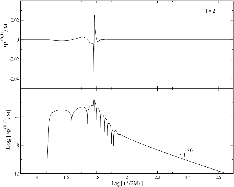
Figure 6.13: Wave form in semi-logarithmic and logarithmic scale of the quadrupolar component ($l=2$) of the axial master function $\Psi^{(0,1)}$ scaled by the stellar mass $M$. The excitation of the first $w$-mode and its strongly damped ringing phase are evident for $1.78\leq\log\left[t/(2M)\right]\leq 1.95$. The late time power-law tail is also in accordance to the theoretical results.

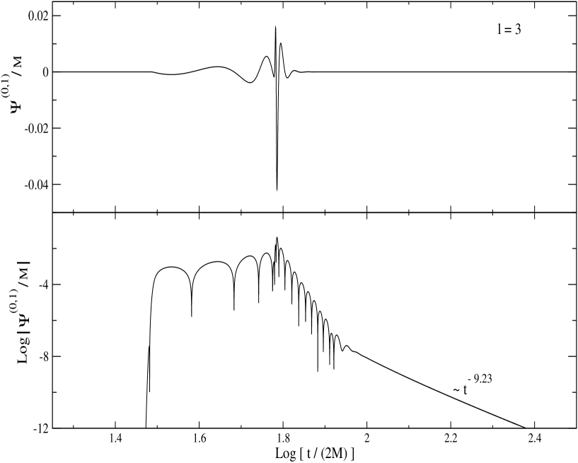
Figure 6.14: Wave form in semi-logarithmic and logarithmic scale of the component $l=3$ of the axial master function $\Psi^{(0,1)}$ scaled by the stellar mass $M$. As for the quadrupolar case, the $w$-mode excitation, the ringing phase and the long term time decay is clearly present.

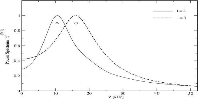
Figure 6.15: Power spectrum of the gravitational signal produced by the scattering of an axial gravitational wave on a spherical non-rotating star. The solid line refers to the quadrupolar term $l=2$ while the dashed line to the $l=3$ case. The frequencies of the first $w$-mode are shown with a triangle for $l=2$ and a circle for $l=3$. The curves are normalized with their maximum values assumed at the peak.

In order to determine the initial profile of the axial velocity we can introduce equation (6.93) into the velocity perturbation (6.88), and obtain:

$$\delta u_{\phi}^{(0,1)}=\frac{A^{2}e^{-\Phi}}{A^{2}+e^{-2\Phi}r^{2}\sin^{2}\theta}\left(r^{2}\sin^{2}\theta\,\Omega_{c}+\sum_{lm}k_{0}^{lm}S_{\phi}^{lm}\right)\,,$$ (6.97)

where we have used the relation (3.91) that connects the frame dragging function with the metric perturbations. It is worth noticing that the axial velocity (6.97) contains as first term the Newtonian j-rotation law up to an exponential factor (hereafter for simplicity, we will call this term the nearly Newtonian j-rotation law), while the second part accounts for the frame dragging. When we introduce equation (6.97) into the inner product (6.96), we can easily determine the expression for the nearly Newtonian term while the relativistic correction requires more attention. In fact the metric variable $k_{0}^{lm}$ is itself the unknown of the differential equation (3.92) and the inner product (6.96) of this term produces quantities which are products of different harmonic indices $(l,m)$. In order to decouple the various terms of the relativistic corrections we will assume that the dominant contributions will be provided by the $k_{0}^{lm}$ which has the same harmonic index as the nearly Newtonian rotation law. When we have determined the harmonic expansion of the nearly Newtonian part, we have found a well posed solution only for $A>e^{-\Phi(R_{s})}R_{s}$. This relation and the values assumed by the metric field $\Phi$ in the stellar model considered in this thesis allow us to give the following estimation:

$$\frac{1}{2}<\frac{A^{2}}{A^{2}+e^{-2\Phi}r^{2}\sin^{2}\theta}\leq 1\,,$$ (6.98)

which can be introduced in the relativistic term of equation (6.97) to give:

$$\delta u_{\phi}^{(0,1)}=\frac{A^{2}r^{2}\sin^{2}\theta\,e^{-\Phi}\,{}}{A^{2}+e^{-2\Phi}r^{2}\sin^{2}\theta}\,\Omega_{c}+\alpha_{0}e^{-\Phi}\sum_{lm}k_{0}^{lm}S_{\phi}^{lm}\,,$$ (6.99)

where $\alpha_{0}\in(0.5,1]$. The expansion of this law in odd-parity vector harmonic provides the following result:

$$\delta u_{\phi,l0}^{(0,1)}=\left\{\begin{array}[]{ll}\alpha_{0}e^{-\Phi}k_{0}^{l0}S_{\phi}^{l0}&\quad\textrm{for}\quad l\quad\textrm{even}\,,\\ \\ \beta^{(0,1)}_{l0}S_{\phi}^{l0}&\quad\textrm{for}\quad l\quad\textrm{odd}\,,\end{array}\right.$$

where the components with odd $l$ are given by the following expression:

$$\beta^{(0,1)}_{l0}=e^{\Phi}\Omega_{c}f_{l0}\left(x,A\right)+\alpha_{0}e^{-\Phi}\,k_{0}^{l0}\,,$$ (6.100)

where $x=re^{-\Phi}$ (not to be confused with the fluid tortoise coordinate). The functions $f_{l0}$ for $l=1$ and $l=3$ are given by the following expressions:

$$\!\!\!\!\!\!\!\!\!\!\!\!f^{(0,1)}_{10} = -3.069A^{2}\left[1-\frac{A^{2}}{x\sqrt{A^{2}+x^{2}}}\ln\frac{\sqrt{x+\sqrt{A^{2}+x^{2}}}}{\sqrt{\sqrt{A^{2}+x^{2}}-x}}\right]\,,$$ (6.101)

$$\!\!\!\!\!\!\!\!\!\!\!\!f^{(0,1)}_{30} = -0.781A^{2}\left[1+7.5\frac{A^{2}}{x^{2}}-\frac{6A^{2}}{x\sqrt{A^{2}+x^{2}}}\left(1+\frac{5}{4}\frac{A^{2}}{x^{2}}\right)\ln\frac{\sqrt{x+\sqrt{A^{2}+x^{2}}}}{\sqrt{\sqrt{A^{2}+x^{2}}-x}}\right],$$ (6.102)

which have been derived by imposing the condition $A>R_{s}e^{-\Phi(R_{s})}$.

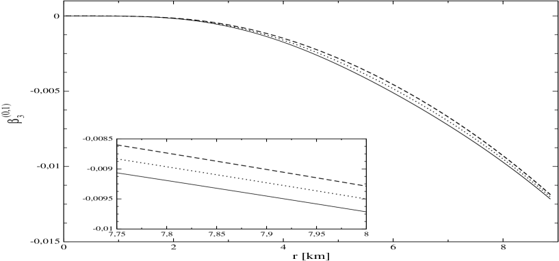
Figure 6.16: Profiles of the $l=3$ component of the axial velocity perturbation $\beta^{(0,1)}_{30}$ in $km$, determined from a j-constant rotation law with $A=15~{}km$ and a $T=10~{}ms$ rotation period at the axis. The axial velocity associated with the nearly Newtonian j-law is shown with a solid line, while the dotted and dashed lines denote the velocity (6.100) with $\alpha=0.5$ and $\alpha=1$ respectively.

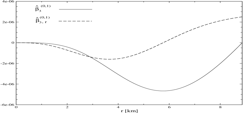
Figure 6.17: Profiles of the $l=3$ components of the axial fluid perturbation $\hat{\beta}^{(0,1)}_{30}$ in $km^{-1}$ (solid line) and its spatial derivative $\hat{\beta}^{(0,1)}_{30,\,r}$ in $km^{-2}$ (dashed lines), determined for a j-constant rotation law with $A=15~{}km$ and a $T=10~{}ms$ rotation period at the axis, and with $\alpha=0$.

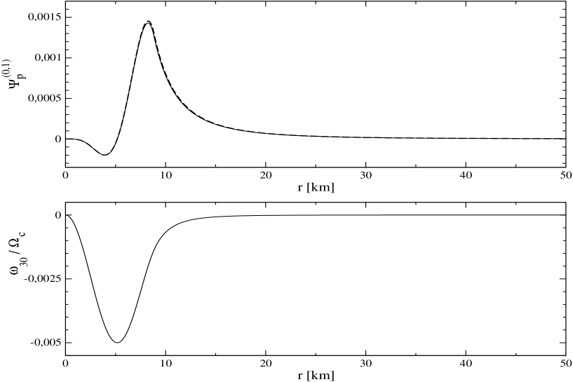
Figure 6.18: The upper panel displays the stationary axial master function $\psi^{(0,1)}_{p}$, in $km$, for a nearly Newtonian j-constant rotation law with $A=15~{}km$ and a period $T=10~{}ms$ at the rotation axis. The solution of equation (3.89) is shown as a solid line while the dashed line is the solution found indirectly by first solving equation (3.92) for the variable $k_{0}^{(0,1)}$ and then using the definition (6.106).

Figure 6.19: The upper panel displays the $l=3$ component of the axial velocity perturbation $\beta^{(0,1)}$, in $km$, for a nearly Newtonian j-constant rotation law with a period $T=10~{}ms$ at the rotation axis and for different values of the differential parameter $A$ (in $km$). The associated solutions of equation (3.89) of the stationary master function $\psi^{(0,1)}_{p}$, in $km$, are shown in the lower panel.

In the limit of $A\rightarrow\infty$, the function $f_{l0}\left(r,A\right)$ behaves correctly, i.e. the nearly Newtonian part assumes the following expressions:

$$\lim_{A\rightarrow\infty}e^{\Phi}\Omega_{c}f_{l0}S_{\phi}^{l0}=\left\{\begin{array}[]{ll}e^{-\Phi}\Omega_{c}r^{2}\sin^{2}\theta&\quad\textrm{for}\quad l=1\,,\\ \\ 0&\quad\textrm{for}\quad l\geq 3\,,\end{array}\right.$$

which corresponds to a uniform rotating configuration, where $\Omega=\Omega_{c}$ is the angular velocity measured at infinity. The aim in this work is the analysis of the gravitational signal produced by the non-linear coupling. Therefore, we will consider only the case $l=3$ as the dipolar term $l=1$ does not produce gravitational waves.

In figure 6.16 is plotted the axial velocity perturbation $\beta_{30}^{(0,1)}$. The figure shows that in the two extreme values of the constant $\alpha_{0}$, the solutions disagree up to ten percent. In the following simulations we will use for simplicity only the nearly Newtonian term and we obtain results which are correct to better than ten percent.

6.4.3 Simulations for axial non-radial perturbations

In this section, we carried out numerical simulations of linear axial perturbations for the two initial configurations described in section 6.4.2.

There are no fluid oscillations associated with linear axial perturbations, therefore these are characterized by pure spacetime oscillations represented in terms of a set of high frequency and strongly damped w-modes. These spacetime modes can be excited dynamically by studying the scattering of an axial gravitational wave on a compact star. This is a standard procedure extensively used in the literature [12, 36]. The gravitational wave can be modelled by an impinging initial Gaussian profile,

$$\left.\Psi_{hom}^{(0,1)}\right|_{t=t_{0}}=A^{(0,1)}e^{-q(r-r_{0})^{2}}\,,$$ (6.103)

where $A^{(0,1)}$ designs the initial wave amplitude, while the constants $q$ and $r_{0}$ control the wide and initial position of the Gaussian respectively. We set up two simulations for the $l=2$ and $l=3$ components of the axial perturbative fields. The initial Gaussian pulse is at $40~{}km$ far from the centre of the star, has an amplitude $A^{(0,1)}=0.1~{}km$ and $q=1.25~{}km^{-2}$. The wave forms determined by an observer at $150~{}km$ are shown in figures (6.13) and (6.14). The scattered signal in both cases exhibits the characteristic excitation of the first $w$-mode at about $\log[t/(2M)]=1.8$ evolution time, followed by the ringing phase which is strongly damped by the emission of gravitational radiation. The ringing of the QNM is more evident in the lower panels of figures (6.13) and (6.14) where the signal is plotted on a logarithmic scale. After this phase, the master function $\Psi_{hom}^{(0,1)}$ shows the typical decreasing behaviour predicted by the theoretical power law $\Psi_{hom}^{(0,1)}\sim t^{-\left(2l+3\right)}$ [26]. For an evolution time of $8~{}ms$ a linear regression of the tail of the signal provides the following values:

$$\Psi_{hom}^{(0,1)}=\left\{\begin{array}[]{ll}t^{-7.06}&\mbox{\qquad for~{}~{}$l=2$\,,}\\ t^{-9.23}&\mbox{\qquad for~{}~{}$l=3$\,.}\end{array}\right.$$ (6.104)

The power law gets closer to the theoretical value for longer evolutions.

The excitation of the first w-modes for the two harmonic indices $l=2,3$ is confirmed by the analysis of the spectral properties of the signal. We perform an FFT of the signal part that starts with the excitation of the spacetime mode. The results in figure 6.15 show the characteristic broad shape of w-modes which is due to the short values of their damping time, respectively $\tau=29.5~{}\mu s$ and $\tau=25.2~{}\mu s$ for the $l=2$ and $l=3$ cases. The curve peaks at the $\nu=10.501~{}kHz$ for the quadrupolar case and at $\nu=16.092~{}kHz$ for the $l=3$ case, which are denoted in figure 6.15 with a triangle and circle respectively. For these two harmonic indices these values are the frequencies of the first curvature $w$-mode, which have been determined by Gualtieri’s numerical code in a frequency domain approach [47].

The other initial configuration for the linear axial perturbation describes a stationary differential rotation induced by the axial velocity perturbation. In particular, the structure of this perturbative framework allows us to investigate the $(l,m)$ component of the axial perturbation $\psi^{(0,1)}$, which is induced by the $(l,m)$ component of the axial velocity perturbation $\beta^{(0,1)}$. As illustrated in section 6.4.2, we are going to implement an axial velocity perturbation described by the function (6.100), which was derived from the relativistic j-constant rotation law. The first point to clarify in equation (6.100) is the amount of the relativistic correction due to its second term with respect to the nearly Newtonian j-constant law. This issue can be studied with equation (3.92) for the metric gauge invariant quantity $k_{0}^{(0,1)}$. We have introduced the functional dependence (6.100) for $\beta^{(0,1)}$ into the source term of equation (3.92) and solved the equation first for a nearly Newtonian rotation law, i.e. $\alpha_{0}=0$, and secondly for $\alpha_{0}=0.5$ and $\alpha_{0}=1$, which are the two extreme values of the relativistic correction to the $l=3$ velocity component. In addition, we choose the following value of the differential rotation parameter $A=15~{}km$ and a $T=10~{}ms$ rotation period at the rotation axis of the star. The choice of $A$ is motivated by the regularity of the $l=3$ component of the axial velocity (see section 6.4.2), that leads to the condition $A>e^{\Phi(R_{s})}~{}R_{s}$. For higher values of $A$, the harmonic components $\beta^{(0,1)}$ with $l>1$ will decrease, as the rotation law approaches the uniform rotation configuration. On the other hand, the angular velocity $\Omega_{c}$ is the physical perturbative parameter that controls the strength of the axial perturbations. Its values must satisfy the requirement imposed by the “slow rotation approximation”, i.e. the dimensionless perturbative parameter $\epsilon=\Omega_{c}/\Omega_{K}\ll 1$, where $\Omega_{K}$ is the Keplerian angular rotation which describes the mass-sheeding limit of the stellar model under consideration. In order to have a simple extimate, we consider the $\Omega_{K}$ of a uniformly rotating star, which can be extimated with the empirical formula [50, 38] which is accurate to better than $10$ percent. This formula is based on the classical value up to a corrrective factor and is given by the following expression:

$$\Omega_{K}\equiv 0.625\,\sqrt{M/R_{s}^{3}}\,,$$ (6.105)

where $M$ and $R_{s}$ are the mass and radius of the non-rotating star in hydrostatic equilibrium. For our stellar model we get $\Omega_{K}=0.0324~{}km^{-1}$ which corresponds to a rotational period $T_{K}=193.996~{}km=0.64~{}ms$. Therefore, the dimensionless parameter is $\epsilon=6.45\times 10^{-2}$.

The numerical integrations of equation (3.92) with the method explained in section 6.4.1 are shown in figure 6.16. The two solutions obtained for $\alpha_{0}=0.5$ and $\alpha_{0}=1$ disagree up to $5$ percent, while the Newtonian differential rotation law is accurate with respect to the relativistic $\alpha_{0}=1$ case to better than $10$ percent. We will use the nearly Newtonian rotation law in this and the next sections, being aware that the results could be accurate within ten percent due to the relativistic corrections of the dragging of inertial frame.

The particular solution of the axial master function $\Psi_{p}^{(0,1)}$ can then be determined by equation (3.89), which is shown in figure 6.18 for the same parameter of the j-constant rotation law used above. This solution can also be determined indirectly by first solving equation (3.92) for the metric variable $k_{0}$ and then getting $\Psi_{p}^{(0,1)}$ through the definition (3.83) for the stationary case:

$$\Psi^{(0,1)}_{p}=\left(2k_{0}^{(0,1)}-rk_{0\,,\,r}^{(0,1)}\right)e^{-\left(\Phi+\Lambda\right)}\,.$$ (6.106)

The indirect solution, which is shown in figure 6.18 as a dashed line, reproduces the solution obtained with the direct method with a maximum error less than $2.3$ percent. In the lower panel of figure 6.18, we show the $l=3$ component of the frame dragging function $\omega_{30}$, which has been found from equation (3.91).

So far, we have used a rotation law with a rotation period at the axis fixed at $T=10~{}ms$. However, the linearity of equation (3.89) allows us to determine the solutions $\Psi_{p}^{(0,1)}$ with a simple rescaling. Let $\left.\Psi_{p}^{(0,1)}\right|_{T_{1}}$ be a solution related to a differential rotation period $T_{1}$. The solution corresponding to a rotational period $T_{2}$ is given by:

$$\left.\Psi_{p}^{(0,1)}\right|_{T_{2}}=\frac{T_{1}}{T_{2}}\,\left.\Psi_{p}^{(0,1)}\right|_{T_{1}}\,.$$ (6.107)

In figure 6.19, we show the effects of the differential parameter $A$ on the profile of the axial velocity $\beta^{(0,1)}$ for $\alpha_{0}=0$ (6.100) and the particular solution of the master function$\Psi_{p}^{(0,1)}$, determined by equation (3.89). The $l=3$ axial velocity and master function decrease for higher values of $A$, when the star tends to a uniform rotational configuration and the only non-vanishing component is the $l=1$. In addition, we have noticed that for $A>100~{}km$ the axial velocity is not accurately described by the expressions (6.101) and (6.102), as it has an irregular behaviour near the origin due to appearence of high peaks.

The rotation energy associated with the differential rotation can be determined with the following equation [53]:

$$E^{(0,1)}=\frac{1}{2}\int_{0}^{R_{s}}dr\int_{0}^{\pi}d\theta\,2\pi r^{4}\sin\theta^{3}\left(\bar{\rho}+\bar{p}\right)e^{\Lambda-\Phi}\Omega\left(\Omega-\omega\right)\,.$$ (6.108)

By neglecting the dragging of the inertial frame $\omega$ we can determine an upper limit of the rotational energy [53]:

$$E^{(0,1)}_{rot}=\frac{1}{2}\int_{0}^{R_{s}}dr\int_{0}^{\pi}d\theta\,2\pi r^{4}\sin\theta^{3}\left(\bar{\rho}+\bar{p}\right)e^{\Lambda-\Phi}\Omega^{2}\,,$$ (6.109)

where $E^{(0,1)}\leq E^{(0,1)}_{rot}$. Furthermore, this expression can be expanded in tensor harmonic as follows:

$$E^{(0,1)}_{rot}=\sum_{l\geq 1}\frac{l\left(l+1\right)}{2\left(2l+1\right)}\int_{0}^{R_{s}}dr\,4\pi\left(\bar{\rho}+\bar{p}\right)e^{\left(\Lambda+\Phi\right)}\left(\beta^{(0,1)}_{lm}\right)^{2}\,$$ (6.110)

where we have applied the following relation $\Omega_{lm}=r^{-2}e^{\Phi}\beta^{(0,1)}_{lm}$, which is valid when the frame dragging function $\omega$ is neglected. The quantities $\Omega_{lm}$ are the harmonic components of the angular velocity,

$$\Omega\left(r,\theta\right)=\sum_{l\geq 1}\Omega_{lm}S_{lm}^{\phi}\,.$$ (6.111)

The upper limit of the $l=1,3$ component of the rotational energy for a differential rotation with $A=15~{}km$ and $T=10~{}ms$ is $E^{(0,1)}_{rot,10}=7.90\times 10^{-5}~{}km$ and $E^{(0,1)}_{rot,30}=8.62\times 10^{-7}~{}km$ respectively.

The solutions $\Psi^{(0,1)}_{hom}$ and $k_{0}$ exhibit a second order convergence, while $\Psi^{(0,1)}_{p}$ manifests a convergence of first order. This lower convergence rate is due to the discontinuity of $\Psi^{(0,1)}_{p,\,rr}$ at the stellar surface.

6.5 Non-linear axial oscillations

The dynamical properties of the coupling between the radial and axial non-radial oscillations are described by the solutions of the two inhomogeneous partial differential equations (4.62) and (4.63), where the source terms are present only in the interior spacetime. The initial values adopted for the linear perturbations are able to describe the non-linear coupling for the following configurations: i) a radially pulsating and differentially rotating star, ii) scattering of a gravitational wave on a radially oscillating star. In particular in the former case, we will see that the coupling between the stationary axial velocity with the radial pulsations produces an oscillating $\lambda\epsilon$ corrective term of the redefined axial velocity $\hat{\beta}^{(1,1)}$.

6.5.1 Numerical algorithms

The conservation equation (4.63) for the perturbation $\hat{\beta}^{(1,1)}$ exists only inside the star and is integrated with an up-wind algorithm. The numerical discretization is given by the following expression:

$$\hat{\beta}^{n+1}_{j}=\hat{\beta}^{n}_{j}+{\Delta}t\,e^{\Phi_{j}}\,\left(\Sigma_{\beta}\right)^{n}_{j}$$ (6.112)

where $\left(\Sigma_{\beta}\right)_{j}$ is the second order discrete approximation of the source term given in appendix (D). Thus, the first and second order derivatives that are present in $\left(\Sigma_{\beta}\right)_{j}$ are approximated by second order centered finite difference approximations in the internal grid points and by second order one-sided finite approximations at the origin and stellar surface.

The integration domain of the axial master equation (4.62) is the entire spacetime, where the source $\Sigma_{\psi}$ is present only in the interior spacetime. After several tests, we have found that the simulations of the master function $\Psi^{(1,1)}$ are more accurate when we implement two different numerical methods. An Up-wind algorithm for the interior and a Leapfrog for the exterior, for studying the coupling between the radial pulsations and differential rotation, and a Leapfrog on the whole spacetime for the scattering of an axial gravitational wave on a radially oscillating star. The implementation of these two methods is due to the different properties of the source terms $\Sigma_{\psi}$ and the junction conditions (4.69) for the two cases mentioned above.

In case of coupling between the radial pulsations and axial differential rotation, we prefer to separate the numerical integration of the axial master equation in the interior and exterior spacetime. Furthermore, in order to reduce the numerical noise caused by the discontinuity of the sources at the stellar surface, we implement a first order accurate numerical scheme in the interior spacetime. Therefore, the axial master equation is simulated with two different numerical schemes inside and ouside the star. In the interior, the second order PDE (4.62) is transformed in a system of first order PDEs which will be integrated with a generalization of the Up-wind method [67]. In the exterior, the Regge-Wheeler equation at order $\lambda\epsilon$ is instead updated in time by using a second order Leapfrog method, where we extract the values of $\Psi^{(1,1)}$ and $\Psi^{(1,1)}_{,\,r}$ on the surface with the matching conditions. Let us first describe the interior spacetime. We can define two new quantities as follows:

$$\textrm{\bf{w}}=\psi^{(1,1)}_{int}\,,\qquad\qquad\textrm{\bf{u}}_{1}=\textrm{\bf{w}}_{\,t}\,,\qquad\qquad\textrm{\bf{u}}_{2}=\textrm{\bf{w}}_{,\,r}\,,$$ (6.113)

where the variable w has been introduce to reduce the number of indices in the discrete equations. With the definition of the vector $\textrm{\bf{u}}\equiv\left[\,\textrm{\bf{u}}_{1},\,\textrm{\bf{u}}_{2}\,\right]^{T}$ we can write the master wave equation (4.62) in the interior spacetime in the following conservative form:

$$\textrm{\bf{u}}_{,\,t}+\textrm{\bf{F}}_{,\,r}=\textrm{\bf{S}}$$ (6.114)

where the flux is given by

$$\textrm{\bf{F}}=\mathbf{A}\textrm{\bf{u}}\,,$$ (6.115)

and $\mathbf{A}$ is the following 2x2 matrix:

$$\mathbf{A}=-\left(\begin{array}[]{cc}0&v_{gw}^{2}\\ 1&0\end{array}\right)\,.$$

The quantity $v_{gw}=e^{\Phi-\Lambda}$ is the propagation velocity of the gravitational signal, and the source S is a two dimensional vector with the following components:

$$\textrm{\bf{S}}_{1} = -e^{2\Phi}\left(4\pi\left(\bar{p}-\bar{\rho}\right)r+\frac{2m}{r}\right)\textrm{\bf{u}}_{2}+V\textrm{\bf{w}}+16\pi\left(4\pi\rho r^{2}-\frac{m}{r}\right)e^{2\Phi+\Lambda}\hat{\beta}^{(1,1)}$$ (6.116)

$$+16\pi re^{2\Phi-\Lambda}\hat{\beta}^{(1,1)}_{,\,r}+\Sigma_{\psi}\,,$$

$$\textrm{\bf{S}}_{2} = 0\,,$$ (6.117)

where $\Sigma_{\psi}$ are the sources expressed in equation (D.1) and are second order accurate in space. The variable u is updated at every time step by the following differentiating scheme,

$$\textrm{\bf{u}}_{j}^{n+1}=\textrm{\bf{u}}_{j}^{n}-\frac{{\Delta}t}{{\Delta}x}\,\mathbf{A}^{+}\left(\textrm{\bf{u}}_{j}^{n}-\textrm{\bf{u}}_{j-1}^{n}\right)-\frac{{\Delta}t}{{\Delta}x}\,\mathbf{A}^{-}\left(\textrm{\bf{u}}_{j+1}^{n}-\textrm{\bf{u}}_{j}^{n}\right)+{\Delta}t\,\textrm{\bf{S}}^{n}_{j}\,,$$ (6.118)

where the matrices $\mathbf{A^{+}}$ and $\mathbf{A^{-}}$ are given by,

$$\mathbf{A^{+}}=\frac{1}{2}\,\left(\begin{array}[]{cc}v&-v^{2}\\ -1&v\end{array}\right)\,,\qquad\qquad\mathbf{A^{-}}=-\frac{1}{2}\,\left(\begin{array}[]{cc}v&v^{2}\\ 1&v\end{array}\right)\,.$$

The value of the $\psi^{(1,1)}_{int}$ is then obtained from the definition (6.113):

$$\textrm{\bf{w}}^{n+1}_{j}=\textrm{\bf{w}}^{n}_{j}+\frac{\Delta t}{2}\,\left[\left(\textrm{\bf{u}}_{1}\right)^{n+1}_{j}+\left(\textrm{\bf{u}}_{1}\right)^{n}_{j}\right]$$ (6.119)

In the exterior spacetime the system of equation reduces to the Regge-Wheeler equation for the master function $\Psi^{(1,1)}$. This axial wave-like equation is solved with a Leapfrog algorithm as well as we did for the first order axial master equation. We do not write the explicit discrete expression for the variable $\Psi^{(1,1)}$ here as it can be determined directly by equation (6.4.1), where the coefficients are now given by

$$v = e^{\Phi-\Lambda}\,,$$ (6.120)

$$\alpha = e^{2\Phi}\frac{2M}{r^{2}}\,,$$ (6.121)

$$V = e^{2\Phi}\left(\frac{6M}{r^{3}}-\frac{l(l+1)}{r^{2}}\right)\,.$$ (6.122)

The scattering of a gravitational wave on a radially pulsating star is instead studied with a Lepfrog algorithm in the whole spacetime. When we discuss the numerical implementation of the junction conditions for non-linear perturbations (section 6.5.2), we will see that the movement of the stellar surface in a Eulerian gauge leads us to adopt some approximate treatments of the matching conditions. As already explained in section 4.2.2, we have chosen in this work to impose the junction conditions on the surface $\Sigma_{jc}$ which is always well inside the star, even during the phases of maximal contraction. Consequently, the axial junction conditions reduce to the continuity of $\Psi^{(1,1)}$ and its derivatives (4.69). We can then integrate equation (4.62) by using the explicit discrete scheme (6.4.1), where we introduce in addition the second order finite approximation of the source $\Sigma_{\psi}$ in the interior spacetime. We have noticed that the junction conditions are automaticaly satisfied by the simulations.

6.5.2 Boundary and initial conditions

The three non-linear coupling perturbations $\Psi^{(1,1)}$, $\Psi^{(1,1)}_{,t}$ and $\beta^{(1,1)}$ are not all independent on the initial Cauchy surface, because of the presence of not vanishing source terms in the non-linear perturbative equations. A correct initial value for the axial master function $\Psi^{(1,1)}$ must come out from the solution of the coupling axial constraints, as in case of first order axial and polar perturbations in presence of sources [82]. However, since we are more interested in the part of the gravitational wave signal which is driven by the stationary radially oscillating sources, we set a vanishing value for all three coupling perturbations at $t=0$ without solving the constraints. As a result, we will see later that after an initial burst of $w$-mode gravitational waves due to the violation of the constraints the solution relax to the correct periodic solution.

Let us now discuss the boundary conditions. At the origin we implement the conditions (4.67) by applying the same procedure described for the linear perturbations. Hence, we have for the metric variable:

$$\textrm{\bf{w}}_{1}=\textrm{\bf{w}}_{2}\left(\frac{r_{1}}{r_{2}}\right)^{l+1}\,,\qquad\qquad\left(\textrm{\bf{u}}_{1}\right)_{1}=\left(\textrm{\bf{u}}_{1}\right)_{2}\left(\frac{r_{1}}{r_{2}}\right)^{l+1}\,,\qquad\qquad\left(\textrm{\bf{u}}_{2}\right)_{1}=\left(\textrm{\bf{u}}_{2}\right)_{2}\left(\frac{r_{1}}{r_{2}}\right)^{l}\,,\qquad\qquad$$ (6.123)

and for the fluid quantity

$$\hat{\beta}^{(1,1)}_{1}=\hat{\beta}^{(1,1)}_{2}\left(\frac{r_{1}}{r_{2}}\right)^{l+1}\,.$$ (6.124)

At the outermost grid point we implement the outgoing Sommerfeld boundary condition, where the outermost grid point is set far enough from the star in order to not corrupt the gravitational signal extraction with the numerical noise coming from the numerical reflection at the grid buondary.
The internal and external spacetimes are separated by the stellar surface, where the matching conditions have to be imposed in order to connect the physical and geometrical descriptions between the interior and exterior spacetime. In an Eulerian gauge, the perturbed surface could not coincide with the surface of the equilibrium configuration. Therefore, when we compare near the surface the perturbations and background tensor fields related to a same physical quantities some problems can arise. Let us for instance consider radial pulsations of a static star, and a point $x_{P}$, which is in the region between the static and perturbed surface during a contraction phase of the star $x(t)<x_{P}<R_{s}$, where $x(t)=R_{s}+\lambda\xi^{(1,0)}$ and $\xi^{(1,0)}$ is the Lagrangian displacement of radial perturbations. During this dynamical phase $x_{P}$ is outside the star, then the mass energy density $\rho$ should vanish there. However, when we determine at $x_{P}$ the Eulerian perturbation

$$\rho^{(1,0)}=\rho-\bar{\rho}$$ (6.125)

where $\bar{\rho}$ is the background density, we find this unphysical value $\rho^{(1,0)}=\bar{\rho}<0$. At any perturbative order, the dynamical properties of the perturbation fields depend on the quantities which have been determined at previous perturbative orders. Therefore, the introduction of this negative values for the density into the $\lambda\epsilon$ perturbative equations could leads to an unphysical description of the non-linear perturbations. This issue can be solved with different methods [101]. For instance, one may add to the stellar model an atmosphere of low density, which extends beyond the size of the neutron star. Otherwise, one can adopt a Lagrangian gauge for the perturbative description. In this case, the perturbed and background surfaces concide and the energy density would get the correct value

$$\Delta\rho^{(1,0)}=\rho^{(1,0)}+\pounds_{\xi^{(1,0)}}\,\rho\geq 0\,,$$ (6.126)

where the vanishing value is taken at the background stellar surface. Alternatively, we can impose the junction conditions on the hypersurface (4.55), which remains always inside the star. With this method we remove the outer layers of the star, but since the density in this region is extremely low the mass neglected is less than one percent. Therefore, the wave forms and spectra of the gravitational signal are still well approximated by this procedure. The position of the junction hypersurface $\Sigma_{jc}$ is evaluated as follows: i) we evolve the radial perturbations and determine the maximum movement of the surface with the Lagrangian displacement $\xi^{(1,0)}_{sf}$. The values for the particular initial conditions used in our evolution are written in table 6.4. ii) Then, we place the surface $\Sigma_{jc}$ at the first grid point that remains inside the star during the evolution. It is worth remarking that for an $r$-grid of dimension $J_{r}=200$, the values of $\xi^{(1,0)}_{sf}$ in table 6.4 leads to neglect only one point, i.e. the junction conditions can be imposed at grid point $J_{jc}=199$. However, since the source of the axial master equation (4.62) has its maximal amplitude at the stellar surface, this removal of a grid point induces a error of about five percent in the gravitational signal.

For the coupling between radial pulsation and differential rotation, we impose the continuity of the metric variable $\Psi^{(1,1)}$ and the relation (4.69) for $\Psi^{(1,1)}_{,\,r}$. For the latter condition we discretize the sided external derivative with a first order approximation in order to get the appropriate value of the master function $\Psi^{(1,1)}$ in the first point outside the junction surface $\Sigma_{jc}$:

$$\psi^{ext}_{J_{jc}} = \textrm{\bf{w}}_{J_{jc}}\,,$$ (6.127)

$$\psi^{ext}_{J_{jc}+1} = \psi^{ext}_{J_{jc}}+{\Delta}r\left[\left(\textrm{\bf{u}}_{2}\right)_{J_{jc}}+16\pi\,r\,\left(\hat{\beta}^{(1,1)}\right)_{J_{jc}}\right]\,,$$ (6.128)

	F	H1	H2	H3	H4	H5	H6
$E^{(1,0)}_{n}~{}[10^{-8}~{}km]$	35.9	4.2	1.37	0.62	0.34	0.21	0.14
$\xi^{(1,0)}_{sf}~{}[m]$	12.65	4.02	2.66	2.02	1.64	1.38	1.19

Table 6.4: Energy $E^{(1,0)}_{0}$ and maximum surface displacement $\xi^{(1,0)}_{sf}$ of radial pulsations. These values correspond to the initial conditions (LABEL:Rad_Ic) and (6.65) with $A^{(1,0)}=0.001$. Every evolution has been excited with a single radial mode.

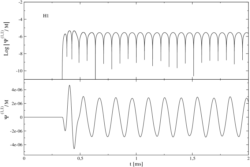
Figure 6.20: Wave form of the axial master function $\psi^{(1,1)}$ scaled by the stellar mass $M$, which describes the coupling between the linear radial pulsations and the axial differential rotation of a neutron star. The rotation is given by a nearly Newtonian j-constant rotation law with a $T=10~{}ms$ period at the rotation axis and $A=15~{}km$, while the radial pulsating dynamics has been excited with the overtone H1. The signal manifests an initial excitation of the first $l=3$ $w$-mode, which is followed by a periodic oscillation driven by the pulsating source terms.

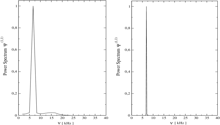
Figure 6.21: Normalized power spectrum of the wave form shown in figure 6.20. The left panel displays the presence of the H1 radial mode and the $l=3$ $w$-mode in the gravitational signal. In the right panel the FFT has been performed for a longer evolution time, thus the energy contained in the H1 peak becomes dominant and the spacetime mode is not visible.

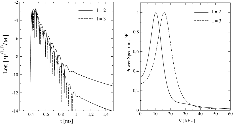
Figure 6.22: The wave forms (left panel) and spectra (right panel) of the master function $\psi$, which corresponds to the toy model studied in section 6.5.3. The presence of an arbitrary transient in the source of equation (6.5.3), which has been induced by a delta function, excites the first $w$-mode.

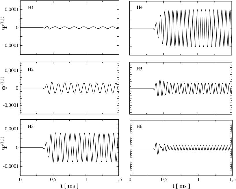
Figure 6.23: Comparison of six wave forms of the axial master function $\psi^{(1,1)}$ given in $km$, where the axial perturbations are described by the same differentially rotating configuration illustrated in figure 6.20. On the other hand, the radial pulsations have been excited each time with one of the six radial overtone (H1-6). The function $\psi^{(1,1)}$, which is plotted on the same scale, shows a resonance effect when the radial perturbations pulsate at H4 overtone, whose frequency is close to the first $w$-mode.

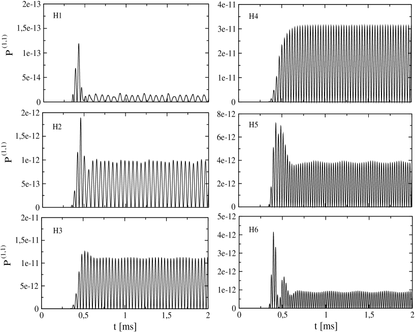
Figure 6.24: For the same six simulations described in figure 6.23, we plot the power emitted in gravitational waves at infinity. The six panels do not have the same scale.

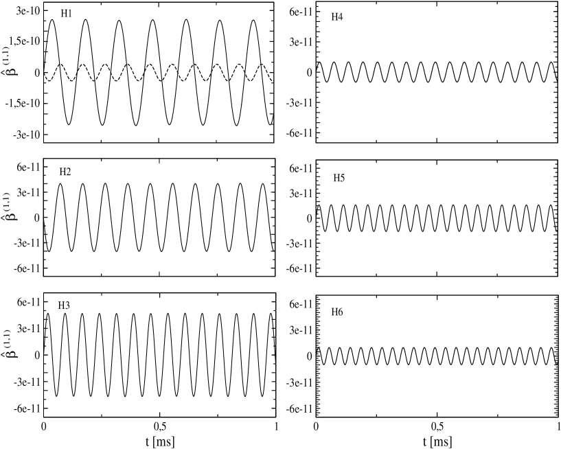
Figure 6.25: Time evolution of the second order fluid perturbation $\hat{\beta}^{(1,1)}$ in $km^{-1}$, which is related to the axial velocity through the definition (4.65). The perturbation $\hat{\beta}^{(1,1)}$ has been averaged at each time step on the interior spacetime with the formula (6.66). The curves plotted in the six panels refer to six evolutions where the radial pulsations have been excited every time with a single overtone of the radial modes. In the upper panel of the first column, we compare the $\hat{\beta}^{(1,1)}$ arising from the H1 (solid line) and H2 (dashed line) radial pulsations. With the exception of the top panel of the first column, all the figures have the same scale.

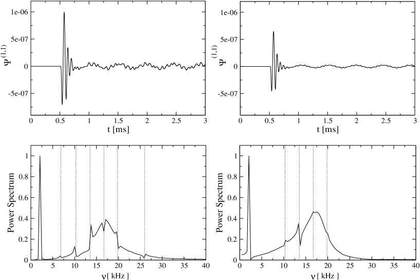
Figure 6.26: Wave forms and spectra of the axial master function $\Psi^{(1,1)}$, in $km$, for the coupling between differential rotation and radial pulsations excited by the F-mode. The left column displays the wave form (top) and spectrum (bottom) for a simulation where the junction conditions have been imposed on a hypersurface at $r=8.64~{}km$. The right column shows the same quantities, but now the matching surface is at $r=7.75~{}km$. In accordance to the results shown in figure 6.23, the excitation of the F-mode and $w$-mode for $l=3$ are evident. In addition, the curves manifest the presence of spurious micro-oscillations that appear at the frequencies of the radial higher overtones (vertical dotted lines). This noise is reduced when the matching is imposed on a more internal hypersurface.

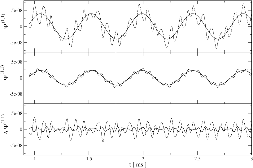
Figure 6.27: The axial master function $\Psi^{(1,1)}$, in $km$, (dashed line) and interpolation function $f^{int}$ (solid line) are plotted for the coupling between differential rotation and radial pulsations excited by the F-mode. In the upper panel the curves are obtained for a simulation where the junction conditions have been imposed on a hypersurface at $r=8.64~{}km$. In the middle panel, the same quantities are now determined by matching at $r=7.75~{}km$. In the lower panel, the difference $\Delta\Psi^{(1,1)}\equiv\Psi^{(1,1)}-f^{int}$ is plotted for $r=8.64~{}km$ (dashed line) and $r=7.75~{}km$ (solid line).

6.5.3 Coupling between radial pulsations and axial differential rotation

In this section, we present the results of the non-linear perturbations which describe the coupling between a stationary differential rotation and radial pulsations. For the particular choice of the initial rotating configuration the non-linear perturbations studied in this section are relative to the harmonic index $l=3$. The axial rotation of the fluid is described with a good approximation by the nearly Newtonian j-constant rotation law which has been derived in section 6.4.2. As in section 6.4.2 and 6.4.3, we have specified the differential parameter ($A=15~{}km$) and the angular velocity at the rotation axis ($\Omega_{c}=2.09~{}10^{-3}~{}km^{-1}$). This value, which corresponds to a $10~{}ms$ rotation period at the axis, is small with respect to the mass shedding limit rotation rate $\Omega_{c}/\Omega_{K}=6.4510^{-2}$. The stationary profile of the axial velocity perturbation $\beta^{(0,1)}$ for the harmonic index $l=3$ is given by the expression (6.100), and has been plotted in the figures (6.16) and (6.19).
The radial pulsations are instead excited for any evolution at $t=0$ by selecting a single normal mode given by equation (LABEL:Rad_Ic), where the initial radial velocity perturbation $\gamma^{(1,0)}$ has the form of equation (6.65) with an initial amplitude $A^{(1,0)}=0.001$. The radial simulations related to these initial conditions provide the maximum Lagrangian displacements shown in table 6.4, which have been determined at the static surface of the star. From these values, we can argue that the region of the spacetime where the perturbed surface of the star moves is really confined in a narrow region around the static equilibrium configuration. Therefore, the issues related to the negative values of the mass-energy density in a Eulerian description can be approximatively described by matching the non-linear perturbations on a surface always contained into the star. For more details see section 6.5.2.

We start by investigating the evolution of the axial master function $\Psi^{(1,1)}$, when the radial perturbations oscillate at the frequency of the first overtone H1. In figure 6.20 we show the wave form for an observer at $100~{}km$ from the stellar centre. This curve presents a first excitation of a typical $w$-mode followed by a monochromatic periodic signal. This interpretation is confirmed by the spectrum associated to this signal. Indeed the left panel of figure 6.21 displays the broad peak of the $w$-mode, which is centered around the frequency $\nu=16.092~{}kHz$, and a narrow peak, which has the same frequency of the first overtone H1 that has been mirrored in the gravitational signal at second order. In the right panel, the FFT of the signal has been performed for a higher number of time cycles where the signal is dominated by the periodic evolution of the source terms. As a result, the energy contained at the frequency of H1 is much higher than that of the curvature mode. The presence of a periodic dynamics which reflects the radial pulsations into these non-linear coupling arises from the structure of the source terms. In fact for a stationary axial perturbation, we can schematically write the sources of equations (4.62) and (4.63) as

$${\cal S}=\sum_{\sigma}{\cal I}^{NR}_{n}\left(t,r\right){\cal J}^{R}_{n}\left(t,r\right)=\sum_{n}{\cal I}^{NR}_{n}\left(r\right){\cal J}^{R}_{n}\left(r\right)e^{i\omega_{n}t}$$ (6.130)

where the superscripts $R$ and $NR$ denote respectively the linear radial and non-radial perturbations and $\omega_{\sigma}$ are the discrete set of radial modes. It is then evident that the dynamics is entirely sustained by the normal modes of the radial perturbations and that the $\lambda\epsilon$ gravitational signal $\Psi^{(1,1)}$ and the axial velocity perturbation $\hat{\beta}^{(1,1)}$ oscillate at the frequencies of the radial modes. This behaviour is expected from the symmetries of the stellar model. In fact, the radial frequencies could be corrected by rotation starting from the perturbative order $\lambda\epsilon^{2}$, as they must be invariant for an inversion of the rotation direction $\Omega\to-\Omega$.
On the other hand, the presence of the first $w$-mode seems to have a different origin. This spacetime mode is only excited during the early phases of the dynamical evolution. As explained in section 6.5.2, this gravitational burst is due to the initial transient in $\Psi^{(1,1)}$, which is produced by the initial constraint violation. In order to confirm that a transient can generate a burst of gravitational wave characterized by the excitation of a $w$-mode, we modify the source of the axial master equation (4.62) with an artificial transient described by a delta function placed in a point inside the star at a given time. This delta function is then immediatly removed after a time step. The wave form and the spectrum of the resulting simulation carried out for the harmonic indices $l=2,3$ are shown in figure 6.22, where the excitation of the first $w$-mode is evident.

When we extend this analysis to simulations where the radial pulsations are excited with higher overtones and with the fundamental mode, the wave forms and the spectra have the same features described for the H1 case. However, an interesting amplification is noticed in the gravitational signal when the radial perturbations pulsate at frequencies close to the axial $w$-mode. In figure 6.23, we show with the same scale the axial master function $\Psi^{(1,1)}$ for six simulations, where the initial data for the radial perturbations are provided each time by one of the first six overtones. It is evident that the function $\Psi^{(1,1)}$ increases in amplitude when the order of the radial normal mode increases from the first to the fourth overtone, while the amplitude decreases for the fifth and sixth overtone. The amplitude of $\Psi^{(1,1)}$ related to the radial H4 evolution results is about sixteen times the amplitude of $\Psi^{(1,1)}$ for a H1 evolution. For this stellar model, the spacetime mode for the harmonic index $l=3$ has frequency $16.092~{}kHz$ which is between the frequencies of the third and fourth overtones, $13.545~{}kHz$ and $16.706~{}kHz$ respectively. In addition, we can notice that this effect is present although the energy contained in the radial pulsations and the maximum displacement of the surface decreases proportionally for higher radial modes (see table 6.4). Considering the structure of the axial master equation (4.62), this amplification is certainly due to a resonance between the axial potential $V$, which contains the properties of the QNM of the spacetime, and the source that is pulsating at the radial eigenfrequencies. In fact, we have noticed that this effect disappears when the axial potential is arbitrarily removed from the equation. In addition, the fluid variable $\hat{\beta}^{(1,1)}$ that obeys the conservation equation (4.63) does not show amplification and decreases proportionally with the order of the radial mode. In analogy with a forced oscillator, the amplification of the signal appears when one of the natural frequencies, determined by the form of the axial potential $V$, is sufficiently close to the frequencies associated with the external force term. Moreover, it is interesting to notice in figure 6.23 that in accordance with the broad spectral peak of the $w$-modes (figure 6.15), this resonance affects a wide frequency band around the $w$-mode.
Consistently with the previous results, the power emitted at infinity by gravitational radiation exhibits the amplification present in the axial master function. In figure 6.24, we determine the rate of the radiate energy for the six simulations which have been described before and were shown in figure 6.23. The power displays two distinct contributions: i) a first peak which is due to the energy emitted by the first $w$-mode which comes out from the initial constraint violation, ii) the periodic emission due to the pulsations of the source. However, the relative strengh of these two effects changes when we excite the radial oscillations with different eigenmodes. In fact, the periodic emission first increases proportionally with the order of the radial overtone excited (H1, H2 ,H3). In correspondence with the H4 radial overtone it reaches its maximum and dominate completely the radiation, and eventually it decreases for the H5 and H6 overtones.

Now, we can study the coupling between differential rotation and radial pulsations that oscillate at the fundamental frequency F-mode. From the previous analyses, we can expect a gravitational signal with at initial excitation of the axial $w$-mode, which is immediately followed by periodic pulsations with the F-mode frequency which are driven by the source. In addition, the axial potential $V$ should lower the second part of the signal as the F-mode frequency is far from the first $w$-mode. This expected behaviour is present in the wave forms shown in the upper panels of figure 6.26. Unfortunately, the periodic part of the signal exhibits also some micro-oscillations. They are the spurious numerical oscillations discussed in section 6.3.4, which arise from the regions at low density near the stellar surface and that seem to depend on the profile of the eigenfunction. The signal can be partially improved by neglecting the outer layers of the star. In the left column of figure 6.26 the junction conditions have been imposed on the hypersurface at radial coordinate $r=8.64~{}km$, which corresponds to neglect the $0.3~{}\%$ of the stellar gravitational mass. The waveform (upper panel) and the spectrum (lower panel) clearly diplay the corruption of the signal due to the numerical oscillations, which appear at the frequencies of the radial mode overtones. In the right column, the matching surface is at $r=7.75~{}km$ and the mass neglected is the $6.3~{}\%$ of the total mass of the star. Despite the lower amplitude of the oscillations we can now notice that the waveform and spectrum are closer to the expected form and the numerical noise is reduced. In the spectrum, we can distinguish the excitation of the F-mode and $l=3$ $w$-mode as well as some small peaks due to the numerical noise, especially at the frequency $\nu=13.4~{}kHz$. In order to estimate the error introduced by the micro-oscillations in the “expected” wave forms, we first proceed to eliminate the first part of the signal characterized by the initial transient. Then we interpolate the periodic part of the wave form with a trigonometric function,

$$f^{int}=c_{0}\sin\left(2\pi~{}\nu_{F}t+c_{1}\right)\,$$ (6.131)

where $\nu_{F}$ is the F mode radial frequency and $c_{0}$ and $c_{1}$ are two free parameters, which are determined by the interpolation algorithm. It is worth noticing that the interpolation functions for the two signals shown in figure 6.26 will be in general different, since the amplitude of the wave form depends on the position of the matching surface. Thus, we separately estimate the deviation between the evolved wave form and its interpolation function $f^{int}$ by using the following expression:

$$<\Delta\Psi>\equiv\sqrt{\frac{1}{J}\sum_{j=1}^{J}\left(\Psi^{(1,1)}_{j}-f^{int}_{j}\right)^{2}}\,,$$ (6.132)

where $J$ is the number of grid points. Equation (6.132) provides $<\Delta\Psi>=1.76\times 10^{-8}~{}km$ and $<\Delta\Psi>=4.45\times 10^{-9}~{}km$ for the wave forms extracted on the junction surface at $r=8.64~{}km$ and $r=7.75~{}km$ respectively. The corruption of the signal is then reduced in average by a factor of four at $r=7.75~{}km$. This improvement can be also noticed in figure 6.27, where the wave forms and the interpolation functions are shown for the junction conditions at $r=8.64~{}km$ (top panel) and $r=7.75~{}km$ (middle panel), while the deviation $\Delta\Psi^{(1,1)}\equiv\Psi^{(1,1)}-f^{int}$ is shown in the lower panel.

The perturbative approach used in this thesis does not include the back reaction analysis, i.e. the damping of the radial oscillations or the slowing of the stellar rotation due to the energy emitted by the $\lambda\epsilon$ gravitational radiation. This effect could be studied by investigating the third perturbative order, which is beyond the aims of this thesis. However, we can provide a rough extimate of the damping time of the radial pulsations. We can assume that the energy emitted in gravitational waves is completely supplied by the first order radial oscillations, and that the power radiated in gravitational waves is constant in time. Thus the damping time is given by the following expression:

$$\tau^{(1,1)}_{lm}\equiv\frac{E^{(1,0)}_{n}}{<\dot{E}^{(1,1)}_{lm}>}\,,$$ (6.133)

where $E^{(1,0)}_{n}$ is the energy of the radial pulsations relative to the specific initial eigenfunction (see table 6.4), while $<\dot{E}^{(1,1)}_{lm}>$ is the time averaged value of the power emitted by the $\lambda\epsilon$ axial gravitational wave, which has been calculated by averaging equation (4.3). The calculations carried out with the initial data described before for the linear perturbations provide the results reported in table 6.5. From the definition (6.133) and the bilinear dependence of the non-linear perturbations $\lambda\epsilon$, the damping time $\tau^{(1,1)}_{30}$ depends only on the non-radial parameter $\epsilon$, as $\tau^{(1,1)}_{lm}\sim\epsilon^{-2}$. In the third row of table 6.5, we write the damping of the radial pulsations due to the coupling in terms of oscillation periods for any radial mode, namely

$$N_{osc}=\frac{\tau^{(1,1)}_{lm}}{P_{n}}\,,$$ (6.134)

where $P_{n}=\nu_{n}^{-1}$ and $\nu_{n}$ is the eigenfrequency of the radial normal mode.

The $\lambda\epsilon$ non-linear perturbations are bilinear with respect to their perturbative parameters. In order to test this property in the numerical simulations, we have performed a first simulation by fixing a basic rotation period for the axial perturbations $T_{0}=10~{}ms$ and an initial amplitude of the velocity perturbation $A_{0}=0.001$, and we have determined the averaged values of the non-linear perturbations $\Psi^{(1,1)}_{0}$ and $\beta^{(1,1)}_{0}$. Then, we have carried out several simulations with different periods $T_{n}=nT_{0}$, and radial amplitude $A_{m}=mA_{0}$, where $n,m\in\mathbb{N}$. The associated values for $\Psi^{(1,1)}_{k}=k\Psi^{(1,1)}_{0}$ and $\beta^{(1,1)}_{k}=k\beta^{(1,1)}_{0}$, manifest the bilinear character expected as their values scale almost perfectly with the coupling constant $k=mn$. An example is given in figure 6.28, where we have carried out four simulations with different values of the perturbative parameters. In the upper panel, we have maintained fixed the amplitude of the radial pulsations $A^{(1,0)}=0.01$ for the H2 overtone, and we have changed the rotation period of the differential rotation by an order of magnitude. In the lower panel, the rotation rate is fixed at $T_{c}=100~{}ms$ and the radial initial amplitude is modified by an order of magnitude. In both cases, the axial master function $\Psi^{(1,1)}$ scales by a factor of ten. Therefore, the results obtained in this section can be used to extrapolate the values of the non-linear perturbations for different values of the initial perturbative parameters associated with the radial and non-radial perturbations. Of course, this procedure is correct as long as the strength of the parameters is within the range of validity of the perturbative approach.

The simulations for the non-linear perturbations are stable for very long time evolutions and have a first rate order of convergence, as expected from the implementation of the first order accurate Up-wind numerical scheme.

	F	H1	H2	H3	H4	H5	H6
$\dot{E}^{(1,1)}~{}[10^{-13}]$	$1.85\times 10^{-6}$	$6.83\times 10^{-2}$	$4.85$	$56.03$	$157.01$	$19.08$	$4.45$
$\tau^{(1,1)}_{30}~{}[ms]$	$6.49\times 10^{9}$	$20.49\times 10^{3}$	$94.15$	3.69	0.72	3.67	10.51
$N_{osc}$	$1.39\times 10^{10}$	$1.408\times 10^{5}$	$971.58$	$49.99$	12.07	72.78	240.77

Table 6.5: Rate of energy $\dot{E}^{(1,1)}$ emitted in gravitational waves at infinity with the coupling between radial pulsations and axial differential rotation. Estimated values of the damping times $\tau^{(1,1)}_{30}$ and number of oscillation periods $N_{osc}$ necessary for the non-linear oscillations to radiate the whole energy initially contained by the radial modes.

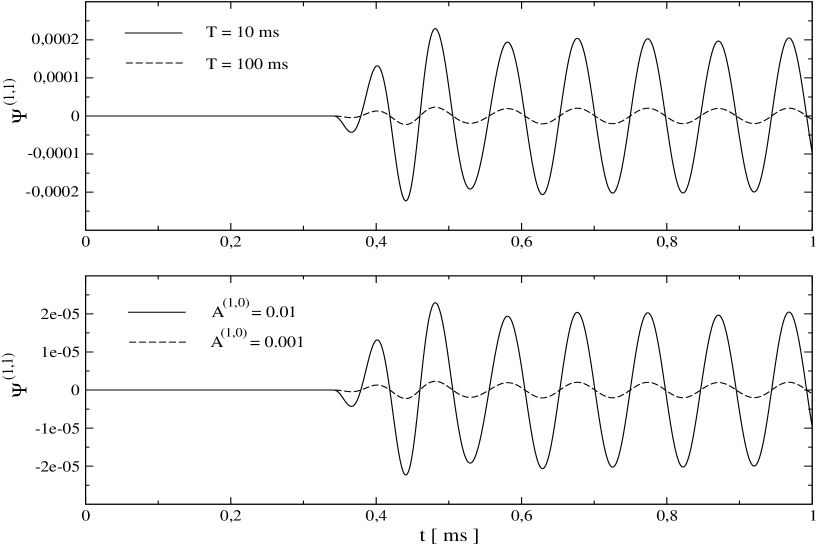
Figure 6.28: Axial master function $\Psi^{(1,1)}$, in $km$, for four different initial values of the first order perturbative parameters. The upper panel displays the wave forms obtained for radial perturbations excited with a H2 overtone of amplitude $A^{(1,0)}=0.01$ and for axial perturbations with rotation periods $T_{c}=10~{}ms$ (solid line) and $T_{c}=100~{}ms$ (dashed line). In the lower panel the rotation period is fixed at $T_{c}=10~{}ms$ and the amplitude of the radial pulsations is changed by an order of magnitude, $A^{(1,0)}=0.01$ (solid line) and $A^{(1,0)}=0.001$ (dashed line).

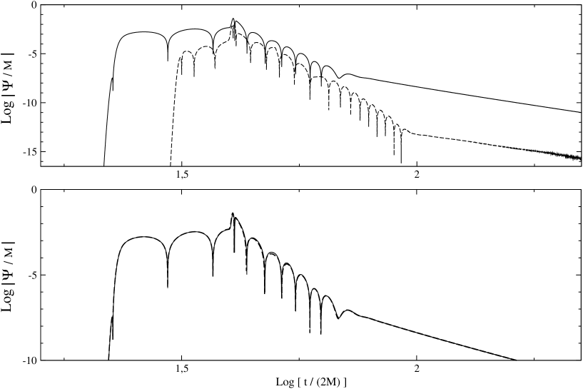
Figure 6.29: Scattering of an axial gravitational wave on a radially oscillating star which is pulsating in the fundamental radial mode. In logarithmic scale, the upper panel displays the wave forms of the first order axial function $\Psi^{(0,1)}$ (solid line) and the second order axial function $\Psi^{(1,1)}$ (dashed line). The lower panel shows again with the solid line the wave forms of $\Psi^{(0,1)}$ and with the dashed line the function $\Psi^{(0,1)}+\Psi^{(1,1)}$.

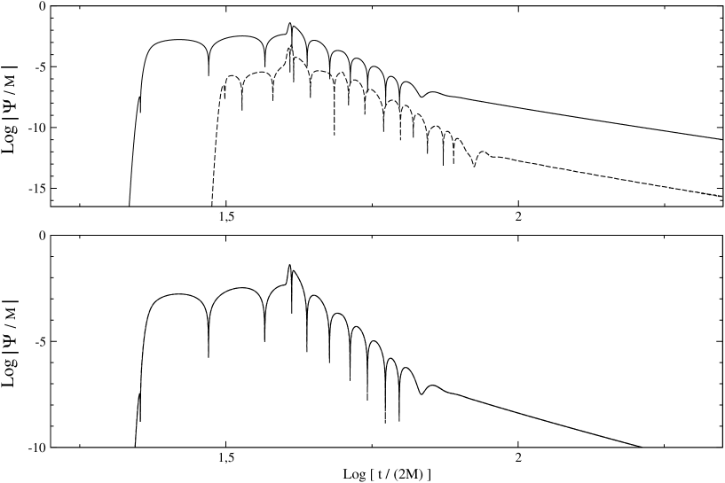
Figure 6.30: With the same notation of figure 6.29, the wave forms are related to the scattering of the gravitational waves on a radially pulsating star where only the first overtone H1 is excited.

Figure 6.31: Scattering of the axial gravitational wave on a radially pulsating star. The solid line in both panels refers to the wave form of $\Psi^{(0,1)}$. In the upper panel the dashed and dotted lines denote the wave forms of $\Psi^{(1,1)}$ for radial pulsations excited by a F-mode and H1-mode respectively. In the lower panel instead, the dashed, dotted and dot-dashed lines describe the wave forms of $\Psi^{(1,1)}$ for radial pulsations excited by H2, H3, and H4 overtones respectively.

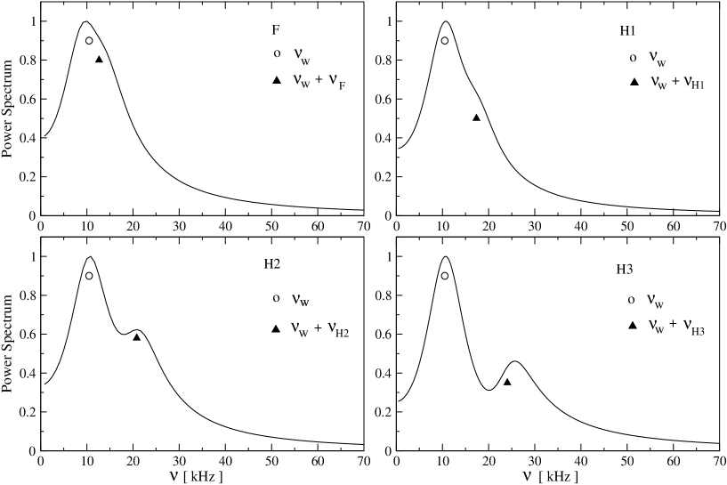
Figure 6.32: Power Spectrum of the wave form $\Psi^{(1,1)}$, which is obtained from the scattering of a axial gravitational wave on a radially pulsating star. The radial pulsations have been excited by selecting in each simulation a particular radial mode, i.e. the F mode and its first three overtones (see labels in the four panels).

6.5.4 Effects of radial pulsations on the scattering of a gravitational wave

In this section, we summarise our study of the scattering of an axial gravitational waves on a radially pulsating spherically symmetric star. The aim is to understand whether the outcoming signal contains some signature of the radially oscillating dynamics of the star. At first order in $\epsilon$, the results are well known and have been re-proposed and briefly discussed in section 6.4.3. The scattered gravitational wave displays an excitation of the first $w$-mode and the associated strongly damped ringing phase.

The initial values for the first order axial perturbations are set up for the harmonic index $l=2$ with the condition (6.87). The velocity perturbation $\beta^{(0,1)}$ then vanishes and the axial master function $\Psi^{(0,1)}$ is given by the Gaussian pulse (6.103) centered at $r_{0}=20~{}km$ with amplitude $A^{(0,1)}=0.1~{}km$ and width parameter $q=1.25~{}km^{-2}$. The radially oscillating phase is excited with the radial eigenfunctions as we have already done in the previous section 6.5.3. However, in order to have a stronger coupling we have increased the initial amplitude of $\gamma^{(1,0)}$ by an order of magnitude, i.e. $A^{(1,0)}=0.01$.

In figures (6.29)-(6.32), we have plotted the first order gravitational master function $\Psi^{(0,1)}$ and the second order correction due to the coupling $\Psi^{(1,1)}$ on a logarithmic scale. The second order signal provides small corrections, less than $2$ percent when the radial pulsations are excited by the F-modes, and less than $0.1$ percent for the higher radial overtones. These corrections do not modify the properties of the wave forms and spectra of the linear analyses. Furthermore, we can notice that the amplification of the signal found in the differential rotating configuration is not present in this case. The fundamental difference between this and the previous case, when the axial perturbation was related to differential rotation, is essentially due to the difference in the properties of the source terms. For the scattering, the source mainly acts for a relatively short period ot time, which is given by the travel time of the linear gravitational wave across the star. After the wave has been scattered, the first order signal still present in the star decreases according to the long time decay power law (section 6.4.3). As a result at second order a longer ringing phase appears which is anyway well below the first order signal. On the other hand, in the coupling between radial pulsations and differential rotation the source terms act periodically into the star forever, as this model does not contain the back-reaction. As a result, the source has more time to couple with the non-radial perturbations.

Although the non-linear coupling does not change the linear results, we can study whether the $\lambda\epsilon$ wave forms and spectra contain some signatures of the radial pulsating dynamics of the star. From figures 6.29 and 6.30, we can notice that for dynamical times $\log\left[t/(2M)\right]\sim 1.70$ the ringing phase presents a small bump, which is due to a small numerical reflection at the stellar surface that appears when the $\lambda\epsilon$ gravitational wave is moving out the star. In particular, this effect is caused by the discontinity of the source terms, which vanish in the exterior spacetime. In addition, the ringing phase of $\Psi^{(1,1)}$ seems to contain some interference effects (see figure 6.32). This suggests the presence of at least two oscillation frequencies. Therefore, we perform an FFT of the signal by selecting the part of the wave form after the numerical reflection. In figure 6.32, the spectra show the presence of the $l=2$ $w$-mode and a non-linear harmonics, whose frequency is the sum of the radial and $w$-mode frequencies. It is worth noticing that this non-linear harmonic exhibits a strong damping and then the characteristic broad shape of the spacetime modes. However, as we have already specified these effects are much lower than the linear results and do not modify the spectra of the linear analysis (see e.g.figure 6.15).

The code for the analysis of the non-linear scattering of a gravitational wave on a radial pulsating star manifests a first order of convergence. This is expected from the discontinuity of $\Psi^{(1,1)}_{,\,rr}$ at the stellar surface, due to the presence of the source terms only in the interior spacetime.

Chapter 7 Conclusions

With the aim of investigating the dynamics of non-linear oscillations of compact stars and the related gravitational radiation, we have presented in this thesis a formalism and a numerical code which enable us to study in the time domain the coupling between the radial and non-radial perturbations of perfect fluid non-rotating compact stars. The formalism for the polar perturbations has been worked out in a first paper [89], while the formalism and the applications to axial perturbations are presented in [90]. The applications of the polar perturbations will be presented in a future work.
In order to have a well-defined framework to consider the gauge dependence of linear and non-linear perturbations, we have found it very convenient to address this topic by using the multi- parameter relativistic perturbation theory introduced in [19, 100]. We have then carried out an expansion of the metric, the energy-momentum tensor and the Einstein and conservation equations in terms of two parameters $\lambda$ and $\epsilon$, where $\lambda$ parameterizes the radial pulsations, $\epsilon$ the non-radial oscillations and the $\lambda\epsilon$ terms describe their coupling. The spherical symmetry of the stellar background allows us to separate in the perturbative tensor fields the time and radial dependence from the angular variables, by using the standard tensor harmonic basis. Therefore, for any harmonic indices $(l,m)$ the linear and the $\lambda\epsilon$ non-linear perturbations have been described by a system of perturbative equations which forms a 1+1 problem, where one dimension is given by the time coordinate and the other by the radial (area) coordinate $r$. The tensor harmonic expansion separates all the perturbative fields in two independent classes, the axial (odd-parity) and polar (even-parity) perturbations, which are defined by their behaviour under a parity transformation. The non-linear perturbative equations and the definition of the gauge invariant non-linear quantities have been derived by using the 2-parameter perturbative theory in connection with the formalism of Gerlach and Sengupta [43], and Gundlach and Martín García [48, 74]. This formalism describes generic one-parameter non-radial perturbations of a time-dependent and spherical symmetric spacetime in terms of a set of gauge invariant perturbations. Our approach consists in exploiting the spherical symmetry of the radial perturbations in order to separate the spherical and time-dependent spacetime of the GSGM formalism in a static background, which describes the equilibrium configuration, and a first order radially pulsating spacetime. We have then fixed the gauge of the radial perturbations and have i) used the GSGM gauge-invariant non-radial $\epsilon$ variables on the static background, and ii) defined new second order $\lambda\epsilon$ variables, describing the non- linear coupling of the radial and non-radial linear perturbations, which are also gauge-invariant for general $\lambda\epsilon$ gauge transformations with the radial gauge fixed. We have then derived the evolution and constraint equations for the non-linear $\lambda\epsilon$ perturbations both for the polar and axial sectors. As expected, in the interior the $\lambda\epsilon$ variables satisfy inhomogeneous linear equations where the homogeneous part is governed by the same linear operator acting on the first order $\epsilon$ non-radial perturbations, while the source terms are quadratic and made of products of $\lambda$ and $\epsilon$ terms. In the exterior the sources vanish and there is no direct coupling, and the whole dynamics is described by the $\lambda\epsilon$ order Zerilli and Regge-Wheeler functions, respectively for the polar and axial perturbations. Thus the effect of the coupling is transmitted from the interior to the exterior through the junction conditions at the surface of the star.
We have given a brief discussion of the boundary conditions, focusing on those at the stellar surface. In order to avoid negative values of the mass energy density near the surface due to the Eulerian description of the radial and non-radial polar perturbations, we have adopted an approximation already used in literature [101, 102, 51], i.e. we have removed the outer layers of the neutron star, which corresponds to neglecting less than one percent of the total gravitational mass of the star. This approximation leads to a description of the second order $\lambda\epsilon$ gravitational radiation which is accurate to better than five per cent.

The perturbations at first order have been studied with the GSGM quantities. However, in some cases we have redefined these variables or changed them for computational purposes. The radial perturbations have been described by four perturbative fields, two metric and two fluid, which obey three first order in time evolution equations and two constraints, as there is a single radial degree of freedom. This allows us to set up either a hyperbolic-elliptic formulation (HEF) or a purely hyperbolic formulation (PHF). The numerical simulations have shown a good accuracy in both cases. The perturbative equations for the polar $\epsilon$ non-radial perturbations and for the polar $\lambda\epsilon$ coupling rely on the hyperbolic-elliptic system of three equations already used in  [81], where the two hyperbolic equations describe respectively the gravitational wave and the sound wave, while the elliptic equation is the Hamiltonian constraint. We have found that this system of equations is more suitable for numerical integration than others available in literature, as the Hamiltonian constraint is used for updating at any time step one of the unknowns of the problem. Therefore, the errors associated with the violation of this constraint are automatically corrected. However, the sound wave equation is only known for first order polar non-radial perturbations. Thus, in order to determine it at the $\lambda\epsilon$ perturbative order, we have first obtained this wave equation for generic non-radial perturbations on a barotropic, time dependent and spherically symmetric background. Then, we have used the 2-parameter expansion and determined the source terms relative to the $\lambda\epsilon$ perturbations. The axial non-radial perturbations for the linear $\epsilon$ and non-linear $\lambda\epsilon$ orders have been studied with a system of two equations, the axial master wave equation and a conservation equation. The former describes the only gauge invariant metric variable of the axial sector, while the latter the axial velocity perturbation. At first perturbative order, the stationary character of the axial velocity allowed us to study separately the dynamical degree of freedom of the spacetime and its stationary part. Linear axial metric perturbations describe the dragging of the inertial frame, the linear axial velocity perturbation represents a stationary differentially rotation.

Since the linear axial velocity induces a stationary differential rotation, the related metric solution describes the dragging of the inertial frame. In the axial sector, we have redefined the axial velocity in order to have a vanishing quantity on the stellar surface. This definition leads to simpler perturbative equations and a better behaviour of the $\lambda\epsilon$ second order source term near the surface of the star.

We have then presented the numerical code for investigating in the time domain the evolution of the axial $\lambda\epsilon$ perturbations. This code is based on finite differencing methods and on standard explicit numerical schemes for integrating partial and ordinary differential equations. The structure of the code reflects the hierarchy of the perturbative frameworks. Starting from the TOV solutions and two independent initial conditions for the radial and non-radial perturbations, the code evolves at any time step the linear radial $\lambda$ and axial non-radial $\epsilon$ perturbations, thus updates the source terms of the $\lambda\epsilon$ perturbative equations, and eventually simulates the evolution of the non-linear perturbations. In order to have more accuracy in the description of the radial pulsations near the surface, we have increased the resolution in this region by adopting the fluid tortoise coordinate, which is necessary only for the radial perturbative equations. Therefore, we have introduced in the numerical code two meshes for describing the radial and non-radial perturbations separately at first order. In order to have source terms calculated at the same grid point, we have also introduced an interpolation that at any time step connects the simulations of the radial pulsations between the two meshes.

In this thesis the static equilibrium configuration is determined by solving the TOV equations for a polytropic equation of state with adiabatic index $\Gamma=2$ and $k=100~{}km^{2}$, and for a central mass energy density $\rho_{c}=3\times 10^{15}~{}g~{}cm^{-3}$. The star then has $M=1.26M_{\odot}$ and $R=8.862~{}km$.
The structure of the radial and axial perturbative equations enables us to set up two independent initial configurations: i) scattering of an axial gravitational wave on a radially pulsating star, ii) a first order differentially rotating and radially pulsating star.
The initial configuration for the radial pulsations has been excited by selecting specific radial eigenmodes. We have chosen an origin of time such that the radial eigenmodes are described only by the eigenfunctions associated with the radial velocity perturbation $\gamma^{(1,0)}$. To this end we have first determined the wave equation for this variable, then we have managed it in order to set up a Sturm-Liouville problem. This eigenvalue problem has been solved with a numerical code based on the shooting method, where the eigenfrequencies of radial modes are accurate to better than 0.2 percent with respect to published values. We have performed some tests for the part of the code dedicated to the radial pulsations. The simulations for any initial radial mode satisfy with high accuracy the Hamiltonian constraint and are stable for very long evolutions. The radial spectrum, which has been determined with a FFT of the time evolution, reproduce the published results with an accuracy to better than 0.2 percent.
For the first order axial perturbations we have excited the dynamical degree of freedom of the spacetime with a standard gravitational wave scattering on the star, where the impinging axial gravitational wave is described by a Gaussian pulse. The tests carried out on the numerical code show that we are able to reproduce the wave forms and the spectra known in literature for the harmonic indices $l=2,3$. The axial differential rotation instead has been described by expanding in vector harmonics the relativistic j-constant rotation law, then taking the first component which is related to the gravitational wave emission, that is $l=3$. We can specify two parameters in the initial profile for the axial velocity perturbations, i.e. the differential parameter $A$ and the angular velocity at the rotation axis $\Omega_{c}$. The value for $A$ has been chosen in order to have a smooth profile and a relatively high degree of differential rotation, as for high $A$ the rotation tends to be uniform and then the $l=3$ component vanishes. We have chosen an angular velocity that corresponds to a $10~{}ms$ rotation period at the axis of the star. For other values of the angular velocity, the linearity of the perturbative equations allows us to get the respective gravitational signal with a simple re-scaling. The relativistic j-constant rotation law contains a term which is related to the dragging of the inertial frame. In order to simplify the expression of our initial condition we have estimated the amount of correction associated with the $l=3$ component of this relativistic term. We have then neglected it, thereby introducing an error of less than ten percent.

For the first initial configuration, i.e. the scattering of an axial gravitational wave on a radially pulsating star, the second order signal provides small corrections, less than $2$ percent when the radial pulsations are excited by the F-modes, and less than $0.1$ percent for the higher radial overtones. These corrections do not modify the properties of the wave forms and spectra of the linear analyses. The second configuration, where the linear axial perturbations describe a stationary differential rotation and the associated frame dragging, produces an new interesting gravitational signal. The wave forms have these properties: i) an excitation of the first $w$-mode at the early stage of the evolution ii) a periodic signal which is driven by the radial pulsations through the source terms. The spectra confirm this picture by showing that the radial normal modes are mirrored in the gravitational signal at non-linear perturbative order. However, the excitation of the $w$-mode at the early stages of the numerical simulations is an unphysical response of the system to the initial violation of the axial constraint equations for the coupling perturbations. Moreover, a resonance effect is present when the frequencies of the radial pulsations are close to the first $w$-mode. For the stellar model considered in this thesis the amplitude of the gravitational wave signal related to the fourth radial overtone is about three orders of magnitude higher than that associated with the fundamental mode. We have also roughly estimated the damping times of the radial pulsations due to the non-linear gravitational emission. Their values radically depend on the presence of resonances. For a $10~{}ms$ rotation period at the axis and $15~{}km$ differential parameter, the fundamental mode damps after about ten billion oscillation periods, while the fourth overtones after ten only. This is not surprising, and shows that the coupling near resonances is a very effective mechanism for extracting energy from the radial oscillations.

It is worthwhile to remark that a possible detection of this gravitational signal could provide new information of the stellar parameters, as the second order gravitational spectra reproduce those of the radial modes of a non-rotating star, which can be determined easily for a large class of equations of state. The numerical code manifests a first order convergence for the simulations of the non-linear axial perturbations arising from the coupling between the first order radial and axial non-radial perturbations.

Future extensions

The implementation of the numerical code for studying the coupling between the radial pulsations and the polar non-radial perturbations is currently under way. The spectrum of the polar non-radial perturbations is richer than the axial case due to the presence of the fluid modes, which may have frequencies lower than the spacetime modes and a longer gravitational damping. As a result, we may expect a more effective coupling with the radial pulsation modes.

Future extension of this work certainly must consider more realistic models of the star, which take into account the effects of rotation, composition gradients, magnetic fields, dissipative effects, etc. In particular, it would be interesting in a protoneutron star to compare the damping rate due to the gravitational radiation produced by the coupling with the strong damping induced by the presence of a high-entropy envelope, which surrounds the newly created neutron star.
New interesting non-linear effects could come out when the star is rotating, mainly due to the different behaviour of the radial and non-radial modes in a rotating configuration. While the radial modes are only weakly affected and their spectrum can be considered almost the same as that of a radially pulsating non-rotating star (when scaled by the central density), the non-axisymmetric modes manifest a splitting similar to that observed in the atomic energy levels due to the Zeeman effect. The rotation has the effect of removing the mode degeneracy of the azimuthal quantum number, which is present in the non-rotating case. The amount and the details of this frequency separation depend on the stellar compactness and rotation rate. We might then expect that for a given stellar rotation rate and compactness the non-radial frequencies should cross the sequence of the radial modes [35]. In this case the frequencies of these two kinds of modes are comparable, and possible resonances or instabilities could influence the spectrum and wave profile of the gravitational wave radiated. The possibility of identifying new resonances in the high frequency gravitational wave spectrum could provide new relations, which can be used to determine the stellar parameters through asteroseismology.

Appendix A Gundlach-Garcia Source terms

In this section we re-write the source terms of the equations of polar non-radial perturbations on a time dependent and spherically symmetric background, which have been found by Gundlach and M. García [48]. These equations are valid for a perfect fluid star with constant entropy along each element fluid trajectory. The equations for a barotropic fluid can be easily determined by neglecting the terms relative to the entropy $s$, its perturbation $\sigma$ and the quantity $C=\left(\frac{\partial p}{\partial s}\right)_{\rho}\,.$

$$S_{\chi} = -2\left[2\nu^{2}+8\pi\rho-{6m\over r^{3}}-2U(\mu-U)\right](\chi+k)+\frac{(l-1)(l+2)}{r^{2}}\chi$$ (A.1)

$$+3\mu\dot{\chi}+4(\mu-U)\dot{k}-(5\nu-2W)\chi^{\prime}-2[2\mu\nu-2(\mu-U)W+\mu^{\prime}-\dot{\nu}]\psi$$

$$+2\eta^{\prime\prime}-2(\mu-U)\dot{\eta}+(8\nu-6W)\eta^{\prime}-\left[-4\nu^{2}+\frac{l(l+1)+8}{r^{2}}+8\nu W\right.$$

$$+\left.4(2\mu U+U^{2}-4W^{2}-8\pi\rho)\right]\eta,$$

$$S_{k} = (1+c_{s}^{2})U\dot{\chi}+[4U+c_{s}^{2}(\mu+2U)]\dot{k}-W(1-c_{s}^{2})\chi^{\prime}-(\nu+2Wc_{s}^{2})k^{\prime}$$ (A.2)

$$-\left[2\left(\frac{1}{r^{2}}-W^{2}\right)+8\pi p-c_{s}^{2}\left(\frac{l(l+1)}{r^{2}}+2U(2\mu+U)-8\pi\rho\right)\right](\chi+k)$$

$$-\frac{(l-1)(l+2)}{2r^{2}}(1+c_{s}^{2})\chi+2[-\mu W(1-c_{s}^{2})+(\nu+W)U(1+c_{s}^{2})]\psi+8\pi{C}\rho\sigma$$

$$-2U\dot{\eta}+2W\eta^{\prime}+\left[\frac{l(l+1)+2}{r^{2}}-6W^{2}+16\pi p-2U(2\mu+U)c_{s}^{2}\right]\eta,$$

$$S_{\psi} = 2\nu(\chi+k)+2\mu\psi+\chi^{\prime}-2\eta(\nu-W)-2\eta^{\prime},$$ (A.3)

$$C_{\gamma} = -W\dot{\chi}+U\chi^{\prime}-(\mu-2U)k^{\prime}+\frac{1}{2}\left[\frac{l(l+1)+2}{r^{2}}+2U(2\mu+U)-2W(2\nu+W)\right.$$ (A.4)

$$\left.+8\pi(p-\rho)\right]\psi-2U\eta^{\prime},$$

$$C_{\omega} = \left[\frac{l(l+1)}{r^{2}}+2U(2\mu+U)-8\pi\rho\right](\chi+k)-\frac{(l-1)(l+2)}{2r^{2}}\chi+2[\nu U+(\mu+U)W]\psi$$ (A.5)

$$+U\dot{\chi}+(\mu+2U)\dot{k}+W\chi^{\prime}-2Wk^{\prime}-2\eta U(2\mu+U),$$

$$C_{\alpha} = 2\mu(\chi+k)+2\nu\psi+\dot{\chi}+2\dot{k}-2\eta(\mu+U),$$ (A.6)

$$S_{\omega} = \left(1+\frac{p}{\rho}\right)\left[-\frac{l(l+1)}{r^{2}}\alpha+\frac{\dot{\chi}+3\dot{k}}{2}+\left(\nu+2W-\frac{\nu}{c_{s}^{2}}\right)\left(\gamma+\frac{\psi}{2}\right)\right]$$ (A.7)

$$+(\mu+2U)\left(c_{s}^{2}-\frac{p}{\rho}\right)\omega-{C}\left[\left(\gamma+\frac{\psi}{2}\right)\frac{s^{\prime}}{c_{s}^{2}}-\sigma(\mu+2U)\right],$$

$$S_{\gamma} = \left(1+\frac{p}{\rho}\right)\left[\frac{\chi^{\prime}+k^{\prime}-2\eta^{\prime}}{2}+\left[c_{s}^{2}(\mu+2U)-\mu\right]\left(\gamma-\frac{\psi}{2}\right)\right]-\nu\left(c_{s}^{2}-\frac{p}{\rho}-\frac{\rho+p}{c_{s}^{2}}\frac{\partial c_{s}^{2}}{\partial\rho}\right)\omega$$ (A.8)

$$-{C}\sigma^{\prime}-\sigma\left[{C}\left(\nu-\frac{s^{\prime}}{c_{s}^{2}}\frac{\partial c_{s}^{2}}{\partial s}\right)+s^{\prime}\frac{\partial{C}}{\partial s}-\nu\left(1+\frac{p}{\rho}\right)\frac{1}{c_{s}^{2}}\frac{\partial c_{s}^{2}}{\partial s}\right]$$

$$-\omega s^{\prime}\left[\frac{\partial c_{s}^{2}}{\partial s}-{C}\left(1+\frac{\rho}{c_{s}^{2}}\frac{\partial c_{s}^{2}}{\partial\rho}\right)\right],$$

$$S_{\alpha} = -\frac{k+\chi}{2}+\eta-c_{s}^{2}(\mu+2U)\alpha+\frac{c_{s}^{2}\omega+{C}\sigma}{1+\frac{p}{\rho}},$$ (A.9)

$$\bar{S}_{\omega} = \left(1+\frac{p}{\rho}\right)\left[\left(-\frac{l(l+1)}{r^{2}}+8\pi(\rho+p)\right)\alpha+\frac{\dot{k}}{2}+(\mu+U)\eta-\mu(\chi+k)\right]$$ (A.10)

$$+(\mu+2U)\left(c_{s}^{2}-\frac{p}{\rho}\right)\omega{C}(\mu+2U)\sigma-\frac{1}{c_{s}^{2}}\left[s^{\prime}{C}+\left(1+{p\over\rho}\right)(\nu-2W{c_{s}^{2}})\right]$$

$$\times\left(\gamma+\frac{\psi}{2}\right)+\nu\left(1+{p\over\rho}\right)\left(\gamma-\frac{\psi}{2}\right),$$

$$\bar{S}_{\gamma} = \left(1+\frac{p}{\rho}\right)\left[\frac{k^{\prime}}{2}+\left(c_{s}^{2}(\mu+2U)-\mu\right)\left(\gamma-\frac{\psi}{2}\right)-\mu\psi-\nu(\chi+k)+(\nu-W)\eta\right]$$ (A.11)

$$-{C}\sigma^{\prime}-\sigma{C}\left[\nu+\frac{s^{\prime}}{{C}}\frac{\partial{C}}{\partial s}-\left(\frac{\nu}{{C}}\left(1+\frac{p}{\rho}\right)+s^{\prime}\right)\frac{1}{c_{s}^{2}}\frac{\partial c_{s}^{2}}{\partial s}\right]$$

$$+\omega\left[\nu\left(\frac{p}{\rho}-c_{s}^{2}\right)+s^{\prime}\left({C}-\frac{\partial c_{s}^{2}}{\partial s}\right)+\left[\nu(\rho+p)+\rho{C}s^{\prime}\right]\frac{1}{c_{s}^{2}}\frac{\partial c_{s}^{2}}{\partial\rho}\right].$$

In this section, we report also the equations relative to the radial perturbations of a time dependent and spherically symmetric star, which have been determined in the radial gauge by Gundlach and M. García [48]. The two fluid evolution equations are given by

$$-\dot{\omega}-{\left(1+\frac{p}{\rho}\right)}\gamma^{\prime} = (\mu+2U){C}\sigma-\omega\left[4\pi\frac{U}{|v|^{2}}(\rho+p)+(\mu+2U)\left(\frac{p}{\rho}-c_{s}^{2}\right)\right]$$ (A.12)

$$- \gamma\left[\frac{{C}s^{\prime}}{c_{s}^{2}}-{\left(1+\frac{p}{\rho}\right)}\left(-4\pi\frac{W}{|v|^{2}}(\rho+p)+\nu+2W-\frac{\nu}{c_{s}^{2}}\right)\right]$$

$$- (\chi-\eta)\left[-\frac{UW}{U^{2}+W^{2}}\frac{{C}s^{\prime}}{c_{s}^{2}}\right.$$

$$+ \left.{\left(1+\frac{p}{\rho}\right)}\left(\mu+U-\nu\frac{UW}{U^{2}+W^{2}}\frac{1+c_{s}^{2}}{c_{s}^{2}}+\frac{U}{2}\frac{|v|^{2}}{U^{2}+W^{2}}\right.\right.$$

$$+ \left.\left.4\pi\frac{UW^{2}}{-U^{4}+W^{4}}(\rho+p)\right)\right]-\eta\frac{U}{|v|^{2}}{\left(1+\frac{p}{\rho}\right)}\left(-\frac{1}{2r^{2}}+4\pi\rho\right),$$

$${\left(1+\frac{p}{\rho}\right)}\dot{\gamma}+c_{s}^{2}\omega^{\prime} = \gamma{\left(1+\frac{p}{\rho}\right)}\left(-4\pi\frac{U}{|v|^{2}}(\rho+p)-\mu+(\mu+2U)c_{s}^{2}\right)$$ (A.13)

$$- \sigma\left[\nu\left({C}-{\left(1+\frac{p}{\rho}\right)}\frac{1}{c_{s}^{2}}\frac{\partial c_{s}^{2}}{\partial s}\right)+4\pi\frac{W{C}}{|v|^{2}}(\rho+p)+s^{\prime}\left(\frac{\partial{C}}{\partial s}-\frac{{C}}{c_{s}^{2}}\frac{\partial c_{s}^{2}}{\partial s}\right)\right]$$

$$- \omega\left[\nu\left(c_{s}^{2}-\frac{p}{\rho}-(\rho+p)\frac{1}{c_{s}^{2}}\frac{\partial c_{s}^{2}}{\partial\rho}\right)+4\pi\frac{Wc_{s}^{2}}{|v|^{2}}(\rho+p)-s^{\prime}\left({C}-\frac{\partial c_{s}^{2}}{\partial s}+\frac{\rho{C}}{c_{s}^{2}}\frac{\partial c_{s}^{2}}{\partial\rho}\right)\right]$$

$$- (\chi-\eta){\left(1+\frac{p}{\rho}\right)}\left(\nu-\mu\frac{UW}{U^{2}+W^{2}}(1+c_{s}^{2})-\frac{2U^{2}W}{U^{2}+W^{2}}c_{s}^{2}+\frac{W}{2}\frac{|v|^{2}}{U^{2}+W^{2}}\right.$$

$$+ \left.4\pi\frac{U^{2}W}{U^{4}-W^{4}}(\rho+p)\right)-\eta\frac{W}{|v|^{2}}{\left(1+\frac{p}{\rho}\right)}\left(\frac{1}{2r^{2}}+4\pi p\right)-{C}\sigma^{\prime},$$

$$\dot{\sigma} = -s^{\prime}\left(\gamma+\frac{UW}{U^{2}+W^{2}}(\eta-\chi)\right).$$ (A.14)

The remaining two metric perturbations $\eta$ and $\chi$ can be obtained from the following constraints:

$$r|v|^{2}D\eta = 4\pi(\rho+p)\left(\chi+\frac{2U^{2}}{|v|^{2}}\eta\right)+8\pi(\rho+p)\frac{2UW}{|v|^{2}}\gamma$$ (A.15)

$$+ \,4\pi\rho\frac{U^{2}+W^{2}}{|v|^{2}}({C}\sigma+(1+c_{s}^{2})\omega),$$

$$r|v|^{2}D\chi = \frac{4UW}{U^{2}+W^{2}}\left(\mu W-\nu U+4\pi\frac{UW}{|v|^{2}}(\rho+p)\right)(\chi-\eta)$$ (A.16)

$$+ \left(-\frac{1}{r^{2}}+8\pi\rho\right)\left(\chi+\frac{2U^{2}}{|v|^{2}}\eta\right)+8\pi(\rho+p)\frac{2UW}{|v|^{2}}\gamma$$

$$+ 8\pi\rho\frac{U^{2}+W^{2}}{|v|^{2}}\omega.$$

Appendix B Sound wave equation

Here, we give the complete form of the sound wave equation  (4.36) for non-radial perturbations on a barotropic, time dependent and spherically symmetric background. This equation is written in terms of the quantities and frame derivatives introduced in the GSGM formalism (2.2).

$$- \ddot{H}+c_{s}^{2}H^{\prime\prime}+\left(\mu+2U\right)\left(c_{s}^{2}-\frac{p}{\rho}-\frac{2}{c_{s}^{2}}\left(\rho+p\right)\frac{dc_{s}^{2}}{d\rho}\right)\dot{H}+\left(\left(2c_{s}^{2}-1\right)\nu+2c_{s}^{2}W\right)H^{\prime}$$ (B.1)

$$+ \left\{\left(\rho+p\right)\left[\left(\rho+p\right)\left(\mu+2U\right)^{2}\frac{1}{c_{s}^{2}}\left(\frac{d^{2}c_{s}^{2}}{d\rho^{2}}-\frac{2}{c_{s}^{2}}\frac{dc_{s}^{2}}{d\rho}^{2}\right)+\left[\left(\mu+2U\right)^{2}\left(2+\frac{\rho-p}{\rho c_{s}^{2}}\right)\right.\right.\right.$$

$$+ \left.\left.\left.\frac{1}{c_{s}^{2}}\left(3U^{2}-\dot{\mu}-\left(2\nu+W\right)W+8\pi p+\frac{1}{r^{2}}\right)\right]\frac{dc_{s}^{2}}{d\rho}+4\pi\left(1+3c_{s}^{2}\right)\right]-\frac{l\left(l+1\right)}{r^{2}}c_{s}^{2}\right\}H$$

$$+ \frac{1}{2}\left(c_{s}^{2}-1\right)\nu\left(\chi^{\prime}-k^{\prime}\right)+c_{s}^{2}\mu\dot{\chi}+\frac{c_{s}^{2}}{2}\left(\mu+2U\right)\left(1+c_{s}^{2}-\frac{p}{\rho}\right)\ \dot{k}+\left\{c_{s}^{2}\left[2\left(2\nu+W\right)W\right.\right.$$

$$+ \left.\left.4\pi\left(\rho-p\right)+2\dot{\mu}-\frac{2}{r^{2}}+\left(1+\frac{p}{\rho}-c_{s}^{2}\right)\mu^{2}-2\left(1+c_{s}^{2}-\frac{p}{\rho}\right)\mu U-2U^{2}\right]-2\nu^{2}\right\}\left(\chi+k\right)$$

$$+ \frac{c_{s}^{2}}{2}\left(\left(1+c_{s}^{2}\right)\mu-2\left(1-c_{s}^{2}\right)U\right)\psi^{\prime}+\left\{\frac{1}{2}\left(1+c_{s}^{2}\right)\left(c_{s}^{2}\mu^{\prime}+\dot{\nu}\right)-\frac{1}{2}\left(\rho+p\right)\frac{dc_{s}^{2}}{d\rho}\left(1-\frac{1}{c_{s}^{2}}\right)\right.$$

$$\times \left.\left(\mu+2U\right)\nu\left[c_{s}^{2}\left(1-\frac{2p}{\rho}+3c_{s}^{2}\right)W+\left[c_{s}^{2}\left(c_{s}^{2}+\frac{p}{\rho}-3\right)+\frac{p}{\rho}\right]\nu\right]U+\left[c_{s}^{2}\left(1-\frac{p}{\rho}+3c_{s}^{2}\right)W\right.\right.$$

$$+ \left.\left.\frac{1}{2}\left[c_{s}^{2}\left(c_{s}^{2}-2\right)+\frac{p}{\rho}\left(1+c_{s}^{2}\right)-3\right]\nu\right]\mu\right\}\psi+c_{s}^{2}\left[2\mu-\frac{p}{\rho}\left(\mu+U\right)\right]\gamma^{\prime}+\left\{\left(1-c_{s}^{2}\right)\left(c_{s}^{2}\mu^{\prime}+\dot{\nu}\right)\right.$$

$$+ \left.\left(\rho+p\right)\left(1+\frac{1}{c_{s}^{2}}\right)\left(\mu+2U\right)\nu\frac{dc_{s}^{2}}{d\rho}+\left[2c_{s}^{2}\left(1+c_{s}^{2}-2\frac{p}{\rho}\right)W-2\left[c_{s}^{2}\left(1+c_{s}^{2}+\frac{p}{\rho}\right)-\frac{p}{\rho}\right]\nu\right]U\right.$$

$$+ \left.\left[2c_{s}^{2}\left(1-c_{s}^{2}-\frac{p}{\rho}\right)W+\left[c_{s}^{2}\left(2-c_{s}^{2}\right)+\frac{p}{\rho}\left(1-c_{s}^{2}\right)-1\right]\nu\right]\mu\right\}\gamma$$

$$+ \left\{\left[8\pi\left(\rho+p\right)c_{s}^{4}+\left(\frac{l\left(l+1\right)}{r^{2}}\frac{p}{\rho}+8\pi\frac{\rho^{2}-p^{2}}{\rho}\right)c_{s}^{2}\right]\left(\mu+2U\right)-2\frac{l\left(l+1\right)}{r^{3}}c_{s}^{2}\ \dot{r}\right\}\alpha=0\,.$$

Appendix C Source terms for the $\lambda\epsilon$ polar perturbative equations

The perturbative equations which describe the coupling between the radial and non-radial polar perturbations (4.37)-(4.42) have long terms that are written in this appendix. For the gravitational wave equation (4.38) the source has the following form:

$${\cal S}_{S} = a_{1}S_{,rr}^{(0,1)}+a_{2}S_{,r}^{(0,1)}+a_{3}S_{,t}^{(0,1)}+a_{4}S^{(0,1)}+a_{5}\left(\psi_{,r}^{(0,1)}-2e^{\Lambda-\Phi}k_{,t}^{(0,1)}\right)+a_{6}k^{(0,1)}$$ (C.1)

$$+a_{7}\psi^{(0,1)}\,,$$

where the coefficients $a_{i}$ are given by

$$a_{1} = 2\left(rS^{(1,0)}-\eta^{(1,0)}\right)e^{-2\Lambda}\,,$$ (C.2)

$$a_{2} = \left[2\left(\Lambda_{,r}-5\Phi_{,r}\right)\eta^{(1,0)}-\left(\left(\Lambda_{,r}-5\Phi_{,r}\right)r+3\right)S^{(1,0)}-\left(\Lambda_{,r}+\Phi_{,r}\right)\left(5-\bar{c}_{s}^{\,-2}\right)H^{(1,0)}\right]{e^{-2\,\Lambda}}$$ (C.3)

$$-4\gamma_{,t}^{(1,0)}e^{-\Phi-\Lambda}\,,$$

$$a_{3} = -4\left(\Lambda_{,r}+\Phi_{,r}\right)\gamma^{(1,0)}e^{-\Lambda-\Phi}-e^{-2\Phi}\eta^{(1,0)}_{,t}+\frac{2}{r}\left(r\gamma^{(1,0)}e^{-\Phi}\right)_{,\,r}e^{-\Lambda}\,,$$ (C.4)

$$a_{4} = -\left\{\frac{4}{r}\left(1+2r\Phi_{,r}\right)\gamma^{(1,0)}_{,t}e^{-\Phi+\Lambda}+2\left[2\Phi_{,r}\left(\frac{1}{r}+2\Phi_{,r}\right)+\frac{2-\left(l(l+1)+2\right)e^{2\Lambda}}{r^{2}}\right.\right.$$ (C.5)

$$\left.\left.+3\frac{\Lambda_{,r}+\Phi_{,r}}{r}\right]\eta^{(1,0)}-\left[\Phi_{,r}+3\Lambda_{,r}+\frac{3-\left(l(l+1)+2\right)e^{2\Lambda}}{r}\right]S^{(1,0)}\right.$$

$$\left.+\left(\Lambda_{,r}+\Phi_{,r}\right)\left[\left(5+\frac{3}{\bar{c}_{s}^{2}}\right)\frac{1}{r}+8\Phi_{,r}\right]H^{(1,0)}\right\}e^{-2\Lambda}\,,$$

$$a_{5} = -2\left[\left(\frac{e^{\Phi}}{r}\gamma^{(1,0)}\right)_{,r}-\left(\Lambda_{,r}+\Phi_{,r}\right)\left(\frac{e^{\Phi}}{r}\gamma^{(1,0)}\right)\right]e^{-2\Lambda-\Phi}\,,$$ (C.6)

$$a_{6} = -\left[\frac{2}{r^{2}}\left(-5+2r(\Phi_{,r}-\Lambda_{,r})+2e^{2\Lambda}\right)S^{(1,0)}+\frac{8}{r^{3}}\left(1+r^{2}\Phi_{,r}^{2}+r\Lambda_{,r}-e^{2\Lambda}\right)\eta^{(1,0)}\right.$$

$$+ \left.\frac{4}{r^{2}}\left(\Lambda_{,r}+\Phi_{,r}\right)\left(2r\Phi_{,r}+\frac{1}{\bar{c}_{s}^{2}}\right)H^{(1,0)}+\frac{8}{r}\Phi_{,r}\gamma^{(1,0)}_{,t}e^{-\Phi+\Lambda}\right]e^{-2\Lambda}\,,$$ (C.7)

$$a_{7} = -\frac{2}{r}\left\{\left(1-\bar{c}_{s}^{2}\right)r\left(\frac{e^{\Phi}}{r}\gamma^{(1,0)}\right)_{,rr}\!\!\!+\left(\frac{e^{\Phi}}{r}\gamma^{(1,0)}\right)_{,r}\left[r\left(\Phi_{,r}-2\Lambda_{,r}\right)+\left(2\Lambda_{,r}r+\Phi_{,r}r-4\right)\bar{c}_{s}^{2}\right.\right.$$

$$+ \left.\frac{\Phi_{,r}}{4\pi}\frac{\Lambda_{,r}+\Phi_{,r}}{\bar{c}_{s}^{2}}\frac{d\bar{c}_{s}^{2}}{d\bar{\rho}}e^{-2\Lambda}\right]+\left[\left(2-2r\Phi_{,r}-3r\Lambda_{,r}\right)\Phi_{,r}-\left(1+r\Lambda_{,r}\right)\Lambda_{,r}+\left(r\left(\Lambda_{,r}^{2}-\Phi_{,r}^{2}\right)\right.\right.$$

$$+ \left.\left.\left.2\Phi_{,r}+5\Lambda_{,r}\right)\,\bar{c}_{s}^{2}+\frac{\Lambda_{,r}+\Phi_{,r}}{\bar{c}_{s}^{2}}\Phi_{,r}\left[r+\frac{e^{-2\Lambda}}{4\pi r}\left(3-\left(\Lambda_{,r}+\Phi_{,r}\right)r\right)\frac{d\bar{c}_{s}^{2}}{d\bar{\rho}}\right]\frac{e^{\Phi}}{r}\gamma^{(1,0)}\right]\right\}e^{-\Phi-2\Lambda}\,.$$

The source of the sound wave equation (4.39) is given by (4.40):

$${\cal S}_{H} = b_{1}H^{(0,1)}_{,rr}+b_{2}H^{(0,1)}_{,tr}+b_{3}H^{(0,1)}_{,t}+b_{4}H^{(0,1)}_{,r}+b_{5}H^{(0,1)}+b_{6}k^{(0,1)}_{,t}+b_{7}rS^{(0,1)}_{,t}$$ (C.9)

$$+ b_{8}\left[k^{(0,1)}_{,r}-\left(rS^{(0,1)}\right)_{,r}\right]+b_{9}\left(rS^{(0,1)}+k^{(0,1)}\right)+b_{10}\gamma^{(0,1)}_{,r}+b_{11}\gamma^{(0,1)}+b_{12}\psi^{(0,1)}_{,r}$$

$$+ b_{13}\psi^{(0,1)}+b_{14}\alpha^{(0,1)}\,,$$

and the expression of the coefficients $b_{i}$ is the following

$$b_{1} = -\left[2\left(\eta^{(1,0)}-rS^{(1,0)}\right)\bar{c}_{s}^{2}+\frac{e^{-2\Lambda}}{4\pi r}\frac{\Lambda_{,r}+\Phi_{,r}}{\bar{c}_{s}^{2}}\frac{d\bar{c}_{s}^{2}}{d\bar{\rho}}H^{(1,0)}\right]e^{-2\Lambda}\,,$$ (C.10)

$$b_{2} = 2\left(1-\bar{c}_{s}^{2}\right)e^{-\Phi-\Lambda}\gamma^{(1,0)}\,,$$ (C.11)

$$b_{3} = -\left\{\frac{e^{-\Lambda}}{r^{3}}\left(-\frac{e^{-2\Lambda}}{2\pi}\frac{\Lambda_{,r}+\Phi_{,r}}{\bar{c}_{s}^{2}}\frac{d\bar{c}_{s}^{2}}{d\bar{\rho}}+\frac{2\bar{c}_{s}^{2}\bar{\rho}-\bar{p}}{\bar{\rho}}r\right)\left(r^{2}\gamma^{(1,0)}e^{\Phi}\right)_{,r}\right.$$ (C.12)

$$+ \left.\left(\Lambda_{,r}+\Phi_{,r}\right)\left(\frac{e^{-2\Lambda}}{2\pi r}\frac{\Lambda_{,r}+\Phi_{,r}}{\bar{c}_{s}^{2}}\frac{d\bar{c}_{s}^{2}}{d\bar{\rho}}-\bar{c}_{s}^{2}+1+\frac{\bar{p}}{\bar{\rho}}\right)\gamma^{(1,0)}e^{\Phi-\Lambda}+\eta^{(1,0)}_{,t}\right\}e^{-2\Phi}\,,$$

$$b_{4} = \frac{1}{4\pi r}\left[\Lambda_{,r}\left(\Lambda_{,r}-\frac{1}{r}\right)-\left(\frac{1}{r}+\Phi_{,r}\right)\left(2\Phi_{,r}+\Lambda_{,r}\right)\right]\frac{1}{\bar{c}_{s}^{2}}\frac{d\bar{c}_{s}^{2}}{d\bar{\rho}}H^{(1,0)}e^{-4\Lambda}$$ (C.13)

$$- \left\{2\left(1-\bar{c}_{s}^{2}\right)H^{(1,0)}_{,r}+2\left[\left(2\Phi_{,r}-\Lambda_{,r}+\frac{2}{r}\right)\bar{c}_{s}^{2}-\Phi_{,r}\right]\eta^{(1,0)}\right.$$

$$+ \left.\left[3\Phi_{,r}+\frac{1}{2r}+\left(\Lambda_{,r}-4\Phi_{,r}-\frac{7}{2r}\right)\bar{c}_{s}^{2}\right]rS^{(1,0)}\right\}{e^{-2\Lambda}}\,,$$

$$b_{5} = -\left\{\left[\frac{e^{-2\Lambda}}{4\pi r^{2}}\left(1-{e^{2\Lambda}}+\Phi_{,r}\Lambda_{,r}r^{2}+\left(\Lambda_{,r}+\frac{5}{2}\Phi_{,r}\right)r\right)\frac{\Lambda_{,r}+\Phi_{,r}}{\bar{c}_{s}^{2}}\frac{d\bar{c}_{s}^{2}}{d\bar{\rho}}-\left(\Lambda_{,r}+\Phi_{,r}\right)\left(1+3\bar{c}_{s}^{2}\right)\right.\right.$$ (C.14)

$$+ \left.\left.\frac{l(l+1)}{r}\bar{c}_{s}^{2}e^{2\Lambda}\right]S^{(1,0)}+\frac{\Lambda_{,r}+\Phi_{,r}}{\bar{c}_{s}^{2}r}\left[\frac{1}{4\pi r}\left(\left(6\bar{c}_{s}^{2}+1+r\Phi_{,r}\right)\frac{\Lambda_{,r}+\Phi_{,r}}{\bar{c}_{s}^{2}}{e^{-2\Lambda}}-\frac{l(l+1)}{r}\right)\frac{d\bar{c}_{s}^{2}}{d\bar{\rho}}\right.\right.$$

$$+ \left.\left.3\bar{c}_{s}^{4}+4\bar{c}_{s}^{2}+1\right]H^{(1,0)}+\frac{e^{-2\Lambda}}{4\pi r}\frac{\Lambda_{,r}+\Phi_{,r}}{\bar{c}_{s}^{2}}\frac{d\bar{c}_{s}^{2}}{d\bar{\rho}}\left[\left(\frac{2}{r}-\Lambda_{,r}+2\Phi_{,r}\right)H^{(1,0)}_{,r}+H^{(1,0)}_{,rr}\right]\right.$$

$$+ \left.\frac{2}{r}\left[\left(\Lambda_{,r}+\Phi_{,r}\right)\left(1+3\bar{c}_{s}^{2}\right)-\frac{l(l+1)}{r}\bar{c}_{s}^{2}e^{2\Lambda}\right]\eta^{(1,0)}\right\}{e^{-2\Lambda}}\,,$$

$$b_{6} = \left\{\left[\left(\Lambda_{,r}+\Phi_{,r}\right)\left(1+\bar{c}_{s}^{2}-{\frac{\bar{p}}{\bar{\rho}}}\right)\bar{c}_{s}^{2}-\left(1-\bar{c}_{s}^{2}\right)\Phi_{,r}\right]\gamma^{(1,0)}e^{\Phi}\right.$$ (C.15)

$$-\left.\frac{\bar{c}_{s}^{2}}{r^{2}}\left(1+\bar{c}_{s}^{2}-\frac{\bar{p}}{\bar{\rho}}\right)\left(r^{2}\gamma^{(1,0)}e^{\Phi}\right)_{,r}\right\}e^{-2\Phi-\Lambda}\,,$$

$$b_{7} = \left\{\left[\left(\Lambda_{,r}+\frac{2}{r}\right)\bar{c}_{s}^{2}+\frac{\Phi_{,r}}{2}\left(1+\bar{c}_{s}^{2}\right)\right]\gamma^{(1,0)}e^{\Phi}-\frac{\bar{c}_{s}^{2}}{r^{2}}\left(r^{2}\gamma^{(1,0)}e^{\Phi}\right)_{,r}\right\}{e^{-2\Phi-\Lambda}}\,,$$ (C.16)

$$b_{8} = -\left[\frac{\Phi_{,r}}{8\pi r}\frac{\Lambda_{,r}+\Phi_{,r}}{\bar{c}_{s}^{2}}\frac{d\bar{c}_{s}^{2}}{d\bar{\rho}}H^{(1,0)}e^{-2\Lambda}+\left(1-\bar{c}_{s}^{2}\right)\left(\Phi_{,r}\eta^{(1,0)}+\frac{1}{2}H^{(1,0)}_{,r}\right)\right]e^{-2\Lambda}\,,$$ (C.17)

$$b_{9} = -\left\{\left[\frac{2}{r^{2}}\left(1-{e^{2\Lambda}}+3r\Phi_{,r}+r\Lambda_{,r}\right)\bar{c}_{s}^{2}-4{\Phi_{,r}}^{2}\right]\eta^{(1,0)}\right.$$ (C.18)

$$+ \left.\left[\left[3\frac{e^{2\Lambda}-1}{r}-2\Phi_{,r}\left(4+r\Lambda_{,r}\right)-3\Lambda_{,r}\right]\bar{c}_{s}^{2}+4r\Phi_{,r}^{2}\right]S^{(1,0)}\right.$$

$$- \left.\frac{\Lambda_{,r}+\Phi_{,r}}{r}\left[1+2\Phi_{,r}r+3\bar{c}_{s}^{2}-\frac{e^{-2\Lambda}}{4\pi r^{2}}\frac{1}{\bar{c}_{s}^{2}}\frac{d\bar{c}_{s}^{2}}{d\bar{\rho}}\left(\left(3\Phi_{,r}+\Lambda_{,r}\right)r+1-e^{2\Lambda}\right)\right]H^{(1,0)}\right.$$

$$+ \left.2\left[2\Phi_{,r}+\left(\Lambda_{,r}-2\Phi_{,r}-\frac{2}{r}\right)\bar{c}_{s}^{2}\right]H^{(1,0)}_{,r}-2\bar{c}_{s}^{2}H^{(1,0)}_{,rr}\right\}e^{-2\,\Lambda}\,,$$

$$b_{10} = \frac{2\bar{c}_{s}^{2}}{r^{2}}\left\{\left[\left(1-{\frac{\bar{p}}{2\bar{\rho}}}\right)\left(\Lambda_{,r}+\Phi_{,r}\right)+\frac{2}{r}\right]\left(r^{2}\gamma^{(1,0)}e^{\Phi}\right)\right.$$ (C.19)

$$- \left.\left(1-{\frac{p}{2\rho}}\right)\left(r^{2}\gamma^{(1,0)}e^{\Phi}\right)_{,r}\right\}e^{-\Phi-2\Lambda}\,,$$

$$b_{11} = -\frac{1}{r^{3}}\left\{2r\bar{c}_{s}^{2}\left(1-\bar{c}_{s}^{2}\right)\left(r^{2}\gamma^{(1,0)}e^{\Phi}\right)_{,rr}+\left[\frac{\Phi_{,r}}{2\pi}\left(\Lambda_{,r}+\Phi_{,r}\right)\frac{d\bar{c}_{s}^{2}}{d\bar{\rho}}{e^{-2\Lambda}}+2\left(\Phi_{,r}+2\Lambda_{,r}+\frac{2}{r}\right)r\bar{c}_{s}^{4}\right.\right.$$ (C.20)

$$- \left.\left.\left(4\left(1+r\Lambda_{,r}\right)+{\frac{\bar{p}}{\bar{\rho}}\left(2+r\Phi_{,r}\right)}\right)\bar{c}_{s}^{2}-\left(2-{\frac{\bar{p}}{\bar{\rho}}}\right)r\Phi_{,r}\right]\left(r^{2}\gamma^{(1,0)}e^{\Phi}\right)_{,r}\right.$$

$$+ \left.\left[-2\left(\Lambda_{,r}+\Phi_{,r}\right)\left(1+\left(\Phi_{,r}-\Lambda_{,r}\right)r\right)\bar{c}_{s}^{4}+\left(\frac{5}{r}-\frac{\Phi_{,r}}{2}\left(2\Phi_{,r}r+7+8r\Lambda_{,r}\right)\right.\right.\right.$$

$$- \left.\left.\left.2\Lambda_{,r}\left(r\Lambda_{,r}-1\right)+\frac{\bar{p}}{\bar{\rho}}\frac{\Phi_{,r}r\left(2\Phi_{,r}r+5\right)+2}{2r}-\frac{e^{2\Lambda}}{2r}\left(1+{\frac{\bar{p}}{\bar{\rho}}}\right)\left(2+\Phi_{,r}r\right)\right)\bar{c}_{s}^{2}\right.\right.$$

$$+ \left.\left.\left(\left(4-{\frac{\bar{p}}{\bar{\rho}}}\right)\left(\Lambda_{,r}+\Phi_{,r}\right)r+4\right)\Phi_{,r}-\frac{e^{-2\Lambda}}{2\pi}\left(\Lambda_{,r}+\Phi_{,r}\right)^{2}\Phi_{,r}\frac{d\bar{c}_{s}^{2}}{d\bar{\rho}}\right]\right.$$

$$\times \left.\left(r^{2}\gamma^{(1,0)}e^{\Phi}\right)\right\}e^{-\Phi-2\Lambda}\,,$$

$$b_{12} = \frac{\bar{c}_{s}^{2}}{2r^{2}}\left\{\left[\left(\Lambda_{,r}+\Phi_{,r}\right)\left(1+\bar{c}_{s}^{2}\right)+\frac{4}{r}\right]\left(r^{2}\gamma^{(1,0)}e^{\Phi}\right)-\left(1+\bar{c}_{s}^{2}\right)\left(r^{2}\gamma^{(1,0)}e^{\Phi}\right)_{,r}\right\}e^{-\Phi-2\Lambda}\,,$$ (C.21)

$$b_{13} = -\frac{1}{r^{2}}\left\{\bar{c}_{s}^{2}\left(1+\bar{c}_{s}^{2}\right)\left(r^{2}\gamma^{(1,0)}e^{\Phi}\right)_{,rr}\!\!+\frac{e^{-2\Lambda}}{4\pi r}\left(\Lambda_{,r}+\Phi_{,r}\right)\Phi_{,r}\left[\left(\Lambda_{,r}+\Phi_{,r}\right)\left(r^{2}\gamma^{(1,0)}e^{\Phi}\right)\right.\right.$$ (C.22)

$$- \left.\left.\left(r^{2}\gamma^{(1,0)}e^{\Phi}\right)_{,r}\right]\frac{d\bar{c}_{s}^{2}}{d\bar{\rho}}\right.$$

$$- \left.\left[\left(2\Lambda_{,r}+\Phi_{,r}\right)\bar{c}_{s}^{4}+\left(\frac{2}{r}+2\Lambda_{,r}+3\Phi_{,r}+\frac{\bar{p}}{\bar{\rho}}\left(\frac{1}{r}-\frac{\Phi_{,r}}{2}\right)\right)\bar{c}_{s}^{2}+\left(2-\frac{\bar{p}}{2\bar{\rho}}\right)\Phi_{,r}\right]\left(r^{2}\gamma^{(1,0)}e^{\Phi}\right)_{,r}\right.$$

$$+ \left.\left[\left(\frac{4}{r}+\frac{\Lambda_{,r}+\Phi_{,r}}{2}\left(6-\frac{\bar{p}}{\bar{\rho}}\right)\right)\Phi_{,r}-\left(\Lambda_{,r}+\Phi_{,r}\right)\left(\Lambda_{,r}-\Phi_{,r}+\frac{1}{r}\right)\bar{c}_{s}^{4}\right.\right.$$

$$+ \left.\left.\left[\frac{1}{2}\left(\Phi_{,r}+\frac{1}{2r}\right)\left(6\Lambda_{,r}+7\Phi_{,r}-\frac{\bar{p}}{\bar{\rho}}\left(\Phi_{,r}-\frac{2}{r}\right)\right)+\frac{2}{r^{2}}-\left(\Lambda_{,r}-\frac{1}{2r}\right)\left(\Lambda_{,r}+\frac{1}{r}\right)\right.\right.\right.$$

$$+ \left.\left.\left.\frac{1}{4r^{2}}\left(1+\frac{\bar{p}}{\bar{\rho}}\right)\left(r\Phi_{,r}-2\right)e^{2\Lambda}\right]\bar{c}_{s}^{2}\right]r^{2}\gamma^{(1,0)}e^{\Phi}\right\}e^{-\Phi-2\Lambda}\,,$$

$$b_{14} = -\frac{\bar{c}_{s}^{2}}{r^{3}}\left\{\left[2\left(\Lambda_{,r}+\Phi_{,r}\right)\left(1+\bar{c}_{s}^{2}-{\frac{\bar{p}}{\bar{\rho}}}\right)+\frac{\bar{p}}{\bar{\rho}}\frac{l\left(l+1\right)}{r}e^{2\Lambda}\right]\left[\left(r^{2}\gamma^{(1,0)}e^{\Phi}\right)_{,r}\right.\right.$$ (C.23)

$$- \left.\left.\left(\Lambda_{,r}+\Phi_{,r}\right)r^{2}\gamma^{(1,0)}e^{\Phi}\right]e^{-2\Lambda}\right.$$

$$- \left.2l\left(l+1\right)\gamma^{(1,0)}e^{\Phi}\right\}e^{-\Lambda-\Phi}\,.$$

The third equation of the system is the Hamiltonian constraint, whose source term has the following form (4.42):

$${\cal S}_{Hamil} = c_{1}\left(k^{(0,1)}_{,rr}-S^{(0,1)}_{,r}\right)+c_{2}k^{(0,1)}_{,r}+c_{3}k^{(0,1)}_{,t}+c_{4}S^{(0,1)}+c_{5}k^{(0,1)}+c_{6}H^{(0,1)}$$ (C.24)

$$+ c_{7}\psi^{(0,1)}_{,r}+c_{8}\psi^{(0,1)}+c_{9}\gamma^{(0,1)}\,,$$

where the coefficients $c_{i}$ are given by

$$c_{1} = rS^{(1,0)}\,,$$ (C.25)

$$c_{2} = \left(\frac{3}{2}S^{(1,0)}+\frac{\Lambda_{,r}+\Phi_{,r}}{\bar{c}_{s}^{2}}H^{(1,0)}\right)\,,$$ (C.26)

$$c_{3} = -\left(\Lambda_{,r}+\Phi_{,r}\right)e^{\Lambda-\Phi}\gamma^{(1,0)}\,,$$ (C.27)

$$c_{4} = -\left(S^{(1,0)}+2\frac{\Lambda_{,r}+\Phi_{,r}}{\bar{c}_{s}^{2}}H^{(1,0)}\right)\,,$$ (C.28)

$$c_{5} = -\frac{2}{r}\frac{\Lambda_{,r}+\Phi_{,r}}{\bar{c}_{s}^{2}}H^{(1,0)}\,,$$ (C.29)

$$c_{6} = -\frac{2}{r}\frac{\Lambda_{,r}+\Phi_{,r}}{\bar{c}_{s}^{2}}\left[1+\frac{1}{\bar{c}_{s}^{2}}-\frac{e^{-2\Lambda}}{4\pi r}\frac{\Lambda_{,r}+\Phi_{,r}}{\bar{c}_{s}^{4}}\frac{d\bar{c}_{s}^{2}}{d\bar{\rho}}\right]H^{(1,0)}\,,$$ (C.30)

$$c_{7} = \frac{2}{r}\gamma^{(1,0)}\,,$$ (C.31)

$$c_{8} = \frac{1}{r^{2}}\left[\left(2-4\Lambda_{,r}r+l\left(l+1\right){e^{2\Lambda}}\right)\gamma^{(1,0)}+2r\gamma_{,r}^{(1,0)}\right]\,,$$ (C.32)

$$c_{9} = -\frac{4}{r}\left(\Lambda_{,r}+\Phi_{,r}\right)\gamma^{(1,0)}\,.$$ (C.33)

Appendix D Source terms for the $\lambda\epsilon$ axial perturbative equations

The equations which describe the coupling between the radial and non-radial axial perturbations are given by the two equations (4.62)-(4.63). Their source terms $\Sigma_{\Psi}$ and $\Sigma_{\beta}$ have the following form:

$$\Sigma_{\Psi} = 2\left(rS^{(1,0)}-\eta^{(1,0)}\right)\,e^{-2\,\Lambda}\Psi^{(0,1)}_{,\,rr}+\left\{4\pi\left(\bar{\rho}+\bar{p}\right)r\,\frac{1-c_{s}^{2}}{c_{s}^{2}}\,H^{(1,0)}\right.$$ (D.1)

$$+ \left.\left[4\pi\,\left(p-\rho\right)r^{2}-1+\frac{4M}{r}\right]S^{(1,0)}+2\,\left[4\pi\,\left(\bar{\rho}-\bar{p}\right)r-\frac{2M}{r^{2}}\right]\eta^{(1,0)}\right\}\,\Psi^{(0,1)}_{,\,r}$$

$$- \left[\eta^{(1,0)}_{,t}+8\pi(\bar{\rho}+\bar{p})re^{\Lambda+\Phi}\gamma^{(1,0)}\right]\Psi^{(0,1)}_{,t}$$

$$+ \left\{4\pi\left(\bar{\rho}+\bar{p}\right)\frac{1-c_{s}^{2}}{c_{s}^{2}}\,H^{(1,0)}+\left[4\pi\left(\bar{\rho}-\bar{p}\right)r-\frac{l\left(l+1\right)+3}{r}+\frac{12M}{r^{2}}\right]S^{(1,0)}{}\right.$$

$$+ {}\left.2\,\left[4\pi\,\left(p-\rho\right)+\frac{l\left(l+1\right)}{r^{2}}-\frac{6M}{r^{3}}\right]\eta^{(1,0)}\right\}\,\Psi^{(0,1)}-8\pi r\left(4\,\eta^{(1,0)}-3\,rS^{(1,0)}\right)\,e^{-\Lambda}\,\hat{\beta}^{(0,1)}_{,\,r}{}$$

$$+ {}\left\{24\pi\left(4\pi\,\bar{p}\,r^{3}+M\right)\,e^{\Lambda}\,S^{(1,0)}-32\pi\,\left(4\pi\bar{p}\,r^{2}+\frac{M}{r}\right)\,e^{\Lambda}\,\eta^{(1,0)}{}\right.$$

$$+ {}\left.16\pi\,r\,e^{-\Lambda}\,H^{(1,0)}_{,\,r}\right\}\hat{\beta}^{(0,1)}$$

$$\Sigma_{\beta} \equiv -\gamma^{(1,0)}\,e^{-\Lambda}\,\hat{\beta}^{(0,1)}_{,\,r}+\left[\left(\left(4\pi\,\rho\,r-\frac{M}{r^{2}}\right)\,e^{2\Lambda}-\frac{2}{r}\right)\gamma^{(1,0)}-\gamma_{,\,r}^{(1,0)}\right]\,e^{-\Lambda}\,\hat{\beta}^{(0,1)}$$ (D.2)

Appendix E Tensor harmonics

In this section we write the even parity (polar) and the odd parity (axial) tensor harmonics, which have been defined in a covariant way in section 2.2.2. The polar scalar spherical harmonics, which satisfy the condition (2.51), are given by the following explicit expression:

$$Y^{lm}\left(\theta,\phi\right)=e^{im\phi}\sqrt{\frac{2l+1}{4\pi}\frac{\left(l-m\right)!}{\left(l+m\right)!}}P_{lm}\left(\cos\theta\right)\,,$$ (E.1)

where $P_{lm}$ are the associated Legendre functions with the harmonic indices $(l,m)$, which are given by

$$P_{lm}\left(x\right)=\left(-1\right)^{m}\left(1-x^{2}\right)^{\frac{m}{2}}\frac{d^{m}}{dx^{m}}P_{l}\left(x\right)=\frac{\left(-1\right)^{m}}{2^{l}~{}l!}\left(1-x^{2}\right)^{\frac{m}{2}}\frac{d^{l+m}}{dx^{l+m}}\left(x^{2}-1\right)^{l}\,,$$ (E.2)

where $x\in\left[-1,1\right]$, and in the last equality we have used the “Rodrigues representation” for the Legendre function $P_{l}\left(x\right)$:

$$P_{l}\left(x\right)=\frac{1}{2^{l}~{}l!}\frac{d^{l}}{dx^{l}}\left(x^{2}-1\right)^{l}\,.$$ (E.3)

It is worth noticing that for axisymmetric stellar perturbations $m=0$, the associated Legendre polynomial $P_{lm}$ reduces to the Legendre polynomial $P_{l}$.
The polar and axial vector harmonic bases are then given by

$$Y_{a}^{lm} = Y^{lm}_{:a}=\left(Y_{,\,\theta}^{lm},\,Y_{,\,\phi}^{lm}\right)\,,$$ (E.4)

$$S_{a}^{lm} = \epsilon_{a}^{~{}b}Y^{lm}_{b}=\left(-\frac{1}{\sin\theta}Y_{,\,\phi}^{lm},\,\sin\theta\,Y_{,\,\theta}^{lm}\right)\,.$$ (E.5)

The tensor harmonics for the polar sector are given by

$$Y_{ab}^{lm}\equiv Y^{lm}\gamma_{ab}\,,\qquad Z^{lm}_{ab}\equiv Y^{lm}_{:ab}+\frac{l(l+1)}{2}Y^{lm}\gamma_{ab}\,,$$ (E.6)

where the explicit expression of the second order covariant derivative of the spherical scalar harmoncis is given by the following expressions:

$$Y^{lm}_{:\,ab} = \left(\begin{array}[]{cc}Y^{lm}_{,\,\theta\theta}&Y^{lm}_{\,,\theta\phi}-\cot\theta\,Y^{lm}_{,\,\phi}\\ \\ Y^{lm}_{\,,\theta\phi}-\cot\theta\,Y^{lm}_{,\,\phi}&Y_{,\,\phi\phi}^{lm}+\sin\theta\cos\theta\,Y^{lm}_{,\,\phi}\\ \end{array}\right)\,,$$ (E.10)

The axial sector has the following tensor harmonics:

$$S^{lm}_{ab}\equiv S^{lm}_{a:b}+S^{lm}_{b:a}\,,$$ (E.11)

where $S^{lm}_{a:b}$ assumes the following form:

$$S^{lm}_{a:\,b} = \left(\begin{array}[]{cc}-\frac{1}{\sin\theta}\left(Y^{lm}_{,\,\theta\phi}-\cot\theta\,Y^{lm}_{,\,\phi}\right)&\sin\theta\,Y^{lm}_{\,,\theta\theta}\\ \\ -\frac{1}{\sin\theta}Y^{lm}_{\,,\phi\phi}-\cos\theta\,Y^{lm}_{,\,\theta}&\sin\theta\left(Y_{,\,\theta\phi}^{lm}-\cot\theta\,Y^{lm}_{,\,\phi}\right)\\ \end{array}\right)\,.$$ (E.15)

The harmonic tensors form an orthogonal basis of the 2-dimensional sphere $S^{2}$. The orthogonality relations for the polar sector are defined as follows:

$$\int d\Omega\left(Y^{lm\,}\right)^{\ast}Y^{l^{\prime}m^{\prime}} = \delta^{ll^{\prime}}\delta^{mm^{\prime}}\,,$$ (E.16)

$$\int d\Omega\,\gamma^{ab}\,\left(Y^{lm\,}_{a}\right)^{\ast}Y^{l^{\prime}m^{\prime}}_{b} = l\left(l+1\right)\delta^{ll^{\prime}}\delta^{mm^{\prime}}\,,$$ (E.17)

$$\int d\Omega\,\gamma^{ab}\gamma^{cd}\,\left(Z^{lm\,}_{ac}\right)^{\ast}Z^{l^{\prime}m^{\prime}}_{bd} = l\left(l+1\right)\frac{l^{2}+l-2}{2}\delta^{ll^{\prime}}\delta^{mm^{\prime}}\,,$$ (E.18)

where $\delta^{ll^{\prime}}$ is the Kronecker delta and the asterisk denotes complex conjugation. For the axial sector the orthogonality conditions are given by

$$\int d\Omega\,\gamma^{ab}\,\left(S^{lm\,}_{a}\right)^{\ast}S^{l^{\prime}m^{\prime}}_{b} = l\left(l+1\right)\delta^{ll^{\prime}}\delta^{mm^{\prime}}\,,$$ (E.19)

$$\int d\Omega\,\gamma^{ab}\gamma^{cd}\,\left(S^{lm\,}_{(a:c)}\right)^{\ast}S^{l^{\prime}m^{\prime}}_{(b:d)} = 2l\left(l+1\right)\left(l^{2}+l-1\right)\delta^{ll^{\prime}}\delta^{mm^{\prime}}\,,$$ (E.20)

where we have denoted $(a:b)=a:b+b:a$.

Appendix F Finite difference approximations

In “finite differencing method” the derivative operators are approximated by finite difference formulae. The finite approximations are based on an appropriate linear combination of the Taylor expansions of the function of interest. In this section we illustrate this procedure only for the first derivative $u^{\prime}=u_{,\,x}$ of a one-dimensional scalar function $u=u(x)$. For higher derivative orders and variable numbers the method is similar. Let $u=u(x)$ be discretized on a one-dimensional mesh of dimension $J$ and increment $\Delta x$,

$$u_{j}=u(x_{j})\qquad\qquad\textrm{for}\qquad j=1,..,J\,.$$ (F.1)

The Taylor expansion of $u_{j+1}$ and $u_{j-1}$ around the grid point $x_{j}$ reads:

$$u_{j+1} = u_{j}+\Delta xu^{\prime}_{j}+\frac{\Delta x}{2}u^{\prime\prime}_{j}+O(\Delta x^{2})\,,$$ (F.2)

$$u_{j-1} = u_{j}-\Delta xu^{\prime}_{j}+\frac{\Delta x}{2}u^{\prime\prime}_{j}+O(\Delta x^{2})\,.$$ (F.3)

Now, when we take their difference and isolate the term $u^{\prime}_{j}$ we obtain:

$$D_{0}u\equiv\frac{u_{j+1}-u_{j-1}}{2\Delta x}+O(\Delta x^{2})\,,$$ (F.4)

where $D_{0}u$ denotes the centered finite difference approximation of the derivative $u^{\prime}_{j}$, which shows a second order accuracy $O(\Delta x^{2})$. For grid points near the surface these centered formulae are not able to approximate derivatives by using only internal points of the mesh. For this aim it is more appropriate to use one-sided approximations of $u^{\prime}$. First order accurate approximation of $u^{\prime}$ is given by the following expressions:

$$D_{+}u\equiv\frac{u_{j+1}-u_{j}}{\Delta x}+O(\Delta x)\,,$$ (F.5)

$$D_{-}u\equiv\frac{u_{j}-u_{j-1}}{\Delta x}+O(\Delta x)\,,$$ (F.6)

which can be determined by the Taylor expansions (F.2) and (F.3).

Second order accuracy is instead reached with the following finite difference formulae:

$$D_{+}u \equiv -\frac{3u_{j}-4u_{j+1}+u_{j+2}}{2\Delta x}+O(\Delta x^{2})\,,$$ (F.7)

$$D_{-}u \equiv \frac{3u_{j}-4u_{j-1}+u_{j-2}}{2\Delta x}+O(\Delta x^{2})\,.$$ (F.8)

The finite expressions of the second derivative $u^{\prime\prime}$ can be determined on the same line as the first order. The centered finite approximation is given by the following expression:

$$D^{2}_{0}u\equiv\frac{u_{j+1}-2u_{j}+u_{j-1}}{\Delta x^{2}}+O(\Delta x^{2})\,,$$ (F.9)

while the one-sided formulae for $u^{\prime\prime}$ are the following:

$$D^{2}_{+}u \equiv \frac{2u_{j}-5u_{j+1}+4u_{j+2}-u_{j+3}}{\Delta x^{2}}+O(\Delta x^{2})\,,$$ (F.10)

$$D^{2}_{-}u \equiv \frac{2u_{j}-5u_{j-1}+4u_{j-2}-u_{j-3}}{\Delta x^{2}}+O(\Delta x^{2})\,.$$ (F.11)

Appendix G Numerical methods

The numerical algorithms used in the simulations are all present in the reference “Numerical Recipes” [91]. Here we briefly illustrate the McCormack scheme that is not mentioned in this reference. Furthermore, we also write the methods used for determing the convergence rate and the norms of the perturbative solutions.

G.1 McCormack algorithm

It is an explicit second order differencing algorithm and a 2-level method. The scheme consists of two computational steps, namely a predictor and a corrector step. For a given partial differential equation of a function $f=f(t,x)$ that we indicate as follows:

$$f_{,\,t}=G\left(f,f_{,\,x},t,x\right)\,,$$ (G.1)

the value of the function $f$ on the new time-slice is updated as follows:
i) Estimator step

$$\tilde{f}_{j}^{n+1}=\Delta t\,G^{n}_{j,j-1}$$ (G.2)

where the source term $G^{n}_{j,j-1}$ is evaluated at $x_{j-1/2}$ by using the values $f_{j-1}^{n}$ and $f_{j}^{n}$.
i) Corrector step

$$\tilde{f}_{j}^{n+1}=f_{j}^{n}+\Delta t\,\frac{1}{2}\left(G^{n}_{j,j-1}+\tilde{G}^{n+1}_{j+1,j}\right)\,,$$ (G.3)

where now the term $\tilde{G}^{n+1}_{j+1,j}$ is determined by the preliminary values $\tilde{f}_{j}^{n+1}$ and $\tilde{f}_{j+1}^{n+1}$.

G.2 Convergence test

The exact solution of a given analytical equation has to be more and more accurately approximated by numerical solutions determined with an increasing resolution of the numerical mesh. In the limit of an infinite dimension of the grid the numerical solution must tend to the exact solution. In addition, the rate of the convergence has to be consistent with the degree of approximation of the numerical method used.

Let $f^{ex}$ be an exact solution of a given equation, and $f^{c}$ and $f^{m}$ the numerical solutions determined respectively on a coarse grid of dimension $J_{c}$ and a medium grid of $J_{m}=2J_{c}$. The deviation of these solutions from the analytical one can be then written as:

$$\Delta f^{c} \equiv \sqrt{\frac{1}{J_{c}}\sum_{j=1}^{J_{c}}\left(f^{c}_{j}-f^{ex}_{j}\right)^{2}}=E_{0}\Delta r^{\sigma}+O(r^{\sigma+1})\,,$$ (G.4)

$$\Delta f^{m} \equiv \sqrt{\frac{1}{J_{c}}\sum_{j=1}^{J_{c}}\left(f^{m}_{j}-f^{ex}_{j}\right)^{2}}=E_{0}\left(\frac{\Delta r}{2}\right)^{\sigma}+O(r^{\sigma+1})\,,$$ (G.5)

where the differences in these two expressions are both evaluated at the points of the coarse mesh. The letter $\sigma$ denotes the accuracy order of the numerical solution and $E_{0}$ is the unknown error term. The ratio of the previous two expressions leads to the following expression:

$$\frac{\Delta f^{c}}{\Delta f^{m}}=2^{\sigma}+O(r^{\sigma+1})\,,$$ (G.6)

thus the convergence factor $\sigma$ is given by

$$\sigma=\frac{\log\left[\Delta f^{c}/\Delta f^{m}\right]}{\log 2}\,.$$ (G.7)

When the exact solution is unknown the convergence test requires three numerical solutions determined on three different grids whose resolution is in the following proportion 1:2:4. Therefore, in the previous expressions we can replace the exact solution $f^{ex}$ with the numerical solution $f^{f}$ obtained on the fine grid of dimension $J_{f}=2J_{m}=4J_{c}$. It is important to remark that in this second case the convergence test informs us of the correct scaling of the numerical error but it does not imply that the numerical solution is going to converge to the true solution.

G.3 Numerical stability and dissipation

The numerical stability and dissipation of the simulations can be monitored by the constancy of the norms, which can be determined for numerical solutions during their time evolution. Let $f_{j}^{n}$ be the finite approximation of a quantity $f$, which has been determined on a one-dimensional grid of dimension $J$ at the $n$ time slice. The $\mathbf{L}_{2}$ norm can then be calculated at any time step as follows:

$$||f||_{2}=\frac{1}{J}\sum_{j=1}^{J}\left(f_{j}^{n}\right)^{2}\,,$$ (G.8)

where we have introduced the division by $J$ for having an expression averaged on the number of grid points.

References

- [1] igec.lnl.infn.it.
- [2] lisa.jpl.nasa.gov.
- [3] www.virgo.infn.it; www.ligo.caltech.edu; www.geo600.uni-hannover.de; tamago.mtk.nao.ac.jp.
- [4] B. Abbott et al. Analysis of first LIGO science data for stochastic gravitational waves. Phys.Rev. D, 69:122004, 2004.
- [5] B. Abbott et al. Analysis of LIGO data for gravitational waves from binary neutron stars. Phys.Rev. D, 69:122001, 2004.
- [6] B. Abbott et al. First upper limits from LIGO on gravitational wave bursts. Phys.Rev. D, 69:102001, 2004.
- [7] B. Abbott et al. Setting upper limits on the strength of periodic gravitational waves from PSR J1939+2134 using the first science data from the GEO 600 and LIGO detectors. Phys.Rev. D, 69:082004, 2004.
- [8] B. Abbott et al. Limits on Gravitational-Wave Emission from Selected Pulsars Using LIGO Data. Phys.Rev. Lett., 94:181103, 2005.
- [9] B. Abbott et al. Upper limits on a stochastic background of gravitational waves. Phys.Rev. D, 95:221101, 2005.
- [10] B. Abbott et al. Upper limits on gravitational wave bursts in LIGO’s second science run. Phys.Rev. D, 72:062001, 2005.
- [11] G. Allen, N. Andersson, K. D. Kokkotas, and B. F. Schutz. Gravitational waves from pulsating stars: Evolving the perturbation equations for a relativistic star. Phys.Rev. D, 58:124012, 1998.
- [12] N. Andersson and K. D. Kokkotas. Gravitational Waves and Pulsating Stars: What Can We Learn from Future Observations? Phys.Rev. Lett., 77:4134, 1996.
- [13] N. Andersson and K. D. Kokkotas. Pulsation modes for increasingly relativistic polytropes. MNRAS, 297:493, 1998.
- [14] N. Andersson and K. D. Kokkotas. Towards gravitational wave asteroseismology. MNRAS, 299:1059, 1998.
- [15] P. Arras, É. É. Flanagan, S. M. Morsink, A. K. Schenk, S. A. Teukolsky, and I. Wasserman. Saturation of the r-Mode Instability. Astrophys.J., 591:1129, 2003.
- [16] E. Balbinski and B. F. Schutz. A puzzle concerning the quadrupole formula for gravitational radiation. MNRAS, 200:43P, 1982.
- [17] J. M. Bardeen, K. P. Thorne, and D. W. Meltzer. A catalogue of methods for studying the normal modes of radial pulsations of general-relativistic stellar models. Astrophys.J., 145:505, 1966.
- [18] E. Berti, F. White, A. Maniopoulou, and M. Bruni. Rotating neutron stars: an invariant comparison of approximate and numerical space-time models. MNRAS, 358:923, 2005.
- [19] M. Bruni, L. Gualtieri, and C. F. Sopuerta. Two-parameter nonlinear space-time perturbations: Gauge transformations and gauge invariance. Class. Quant. Grav., 20:535, 2003.
- [20] M. Bruni, S. Matarrese, S. Mollerach, and S. Sonego. Perturbations of spacetime: Gauge transformations and gauge invariance at second order and beyond. Class. Quant. Grav., 14:2585, 1997.
- [21] M. Cerdonio, L. Conti, J. A. Lobo, A. Ortolan, and J. P. Zendri. Wideband dual sphere detector of gravitational waves. Phys.Rev. D, 87:031101, 2001.
- [22] S. Chandrasekhar. Dynamical instability of gaseous masses approaching the schwarzshild limit in general relativity. Phys.Rev. Lett., 12:114, 1964.
- [23] S. Chandrasekhar. The Dynamical Instability of Gaseous Masses Approaching the Schwarzschild Limit in General Relativity. Astrophys.J., 140:417, 1964.
- [24] S. Chandrasekhar. Solutions of Two Problems in the Theory of Gravitational Radiation. Phys.Rev. Lett., 24:762, 1970.
- [25] S. Chandrasekhar and V. Ferrari. On the non-radial oscillations of a star. Royal Society of London Proceedings Series A, 432:247, 1991.
- [26] E. S. C. Ching, P. T. Leung, W. M. Suen, and K. Young. Wave propagation in gravitational systems: Late time behavior. Phys.Rev. D, 52:2118, 1995.
- [27] T. G. Cowling. The non-radial oscillations of polytropic stars. MNRAS, 101:367, 1941.
- [28] J. P. Cox. Theory of stellar pulsation. Research supported by the National Science Foundation Princeton, NJ, Princeton University Press, 1980.
- [29] C. T. Cunningham, R. H. Price, and V. Moncrief. Radiation from collapsing relativistic stars. I - Linearized odd-parity radiation. Astrophys.J., 224:643, 1978.
- [30] C. T. Cunningham, R. H. Price, and V. Moncrief. Radiation from collapsing relativistic stars. III - Second order perturbations of collapse with rotation. Astrophys.J., 236:674, 1980.
- [31] G. Darmois. Les équations de la gravitation einsteinienne. In Mémorial des Sciences Mathématiques, volume XXV, chapter V. Gauthier-Villars, Paris, 1927.
- [32] S. Detweiler and L. Lindblom. On the nonradial pulsations of general relativistic stellar models. Astrophys.J., 292:12, 1985.
- [33] H. Dimmelmeier, J. A. Font, and E. Muller. Relativistic simulations of rotational core collapse. I. methods, initial models, and code tests. A&A, 388:917, 2002.
- [34] H. Dimmelmeier, J. A. Font, and E. Muller. Relativistic simulations of rotational core collapse. II. collapse dynamics and gravitational radiation. A&A, 393:523, 2002.
- [35] H. Dimmelmeier, N. Stergioulas, and J. A. Font. Nonlinear axisymmetric pulsations of rotating relativistic stars in the conformal flatness approximation. astro-ph/0511394, 2004.
- [36] V. Ferrari and K. D. Kokkotas. Scattering of particles by neutron stars: Time evolutions for axial perturbations. Phys.Rev. D, 62:107504, 2000.
- [37] J. A. Font. Numerical Hydrodynamics in General Relativity. Living Reviews in Relativity, 6:4, 2003.
- [38] J. L. Friedman and J. R. Ipser. On the maximum mass of a uniformly rotating neutron star. Astrophys.J., 314:594, 1987.
- [39] J. L. Friedman and B. F. Schutz. Secular instability of rotating Newtonian stars. Astrophys.J., 222:281, 1978.
- [40] M. Y. Fujimoto. The Evolution of Accreting Stars with Turbulent Mixing. Astrophys.J., 419:768, 1993.
- [41] A. Garat and R. H. Price. Gauge invariant formalism for second order perturbations of Schwarzschild spacetimes. Phys.Rev. D, 61:044006, 2000.
- [42] U. H. Gerlach and U. K. Sengupta. Even parity junction conditions for perturbations on most general spherically symmetric space-times. J. Math. Phys., 20:2540, 1979.
- [43] U. H. Gerlach and U. K. Sengupta. Gauge invariant perturbations on most general spherically symmetric space-times. Phys.Rev. D, D19:2268, 1979.
- [44] U. H. Gerlach and U. K. Sengupta. Junction conditions for odd parity perturbations on most general spherically symmetric space-times. Phys.Rev. D, 20:3009, 1979.
- [45] U. H. Gerlach and U. K. Sengupta. Gauge invariant coupled gravitational, acoustical, and electromagnetic modes on most general spherical space- times. Phys.Rev. D, D22:1300, 1980.
- [46] R. J. Gleiser, C. O. Nicasio, R. H. Price, and J. Pullin. Second order perturbations of a schwarzschild black hole. Class. Quant. Grav., 13:L117, 1996.
- [47] L. Gualtieri, E. Berti, J. A. Pons, G. Miniutti, and V. Ferrari. Gravitational signals emitted by a point mass orbiting a neutron star: A perturbative approach. Phys.Rev. D, D64:104007, 2001.
- [48] C. Gundlach and J. M. Martín-García. Gauge-invariant and coordinate-independent perturbations of stellar collapse. I: The interior. Phys.Rev. D, D61:084024, 2000.
- [49] I. Hachisu. A versatile method for obtaining structures of rapidly rotating stars. Astrophys.J.SS, 61:479, 1986.
- [50] P. Haensel and J. L. Zdunik. A submillisecond pulsar and the equation of state of dense matter. Nature, 340:617, 1989.
- [51] T. Harada, H. Iguchi, and M. Shibata. Computing gravitational waves from slightly nonspherical stellar collapse to a black hole: Odd-parity perturbation. Phys.Rev. D, 68:024002, 2003.
- [52] J. B. Hartle. Slowly Rotating Relativistic Stars. I. Equations of Structure. Astrophys.J., 150:1005, 1967.
- [53] J. B. Hartle. Slowly-Rotating Relativistic Stars.IV. Rotational Energy and Moment of Inertia for Stars in Differential Rotation. Astrophys.J., 161:111, 1970.
- [54] J. B. Hartle and K. S. Thorne. Slowly Rotating Relativistic Stars. II. Models for Neutron Stars and Supermassive Stars. Astrophys.J., 153:807, 1968.
- [55] R. A. Hulse and J. H. Taylor. Discovery of a pulsar in a binary system. Astrophys.J.Let., 195:L51, 1975.
- [56] J. R. Ipser and R. H. Price. Nonradial pulsations of stellar models in general relativity. Phys.Rev. D, 43:1768, 1991.
- [57] W. Israel. Singular hypersurfaces and thin shells in gr. Nuovo Cimento, B44:1, 1966.
- [58] S. Kind, J. Ehlers, and B. G. Schmidt. Relativistic stellar oscillations treated as an initial value problem. Class. Quantum Grav., 10:2137, 1993.
- [59] K. D. Kokkotas and J. Ruoff. Radial oscillations of relativistic stars. A&A, 366:565, 2001.
- [60] K. D. Kokkotas and B. G Schmidt. Quasi-normal modes of stars and black holes. Living Reviews in Relativity, 2:2, 1999.
- [61] K. D. Kokkotas and B. F. Schutz. W-modes - A new family of normal modes of pulsating relativistic stars. MNRAS, 255:119, 1992.
- [62] K. D. Kokkotas and N. Stergioulas. Gravitational waves from compact sources. gr-qc/0506083, 2005.
- [63] H. Komatsu, Y. Eriguchi, and I. Hachisu. Rapidly rotating general relativistic stars. I - Numerical method and its application to uniformly rotating polytropes. MNRAS, 237:355, 1989.
- [64] H. Komatsu, Y. Eriguchi, and I. Hachisu. Rapidly rotating general relativistic stars. II - Differentially rotating polytropes. MNRAS, 239:153, 1989.
- [65] L. D. Landau and E. M. Lifshitz. Mechanics. Course of Theoretical Physics, Oxford: Pergamon Press, 1969, 2nd ed.
- [66] M. Leins, H.-P. Nollert, and M. H. Soffel. Nonradial oscillations of neutron stars: A new branch of strongly damped normal modes. Phys.Rev. D, 48:3467, 1993.
- [67] R. J. LeVeque. Numerical Methods for Conservation Laws. Birkhäuser Verlag, Basel, 1999.
- [68] Y. Levin and G. Ushomirsky. Non-linear r-modes in a spherical shell: issues of principle. MNRAS, 322:515, 2001.
- [69] A. Lichnerowicz. Sur les ondes de choc gravitationnelles. C. R. Acad. Sci., 273:528, 1971.
- [70] L. Lindblom and S. L. Detweiler. The quadrupole oscillations of neutron stars. Astrophys.J.Suppl., 53:73, 1983.
- [71] L. Lindblom, J. E. Tohline, and M. Vallisneri. Nonlinear Evolution of the r-Modes in Neutron Stars. Phys.Rev. Lett., 86:1152, 2001.
- [72] L. Lindblom, J. E. Tohline, and M. Vallisneri. Numerical Evolutions of non-linear r-Modes in Neutron Stars. Phys.Rev. D, 65:084039, 2002.
- [73] J. M. Martín-García and C. Gundlach. All nonspherical perturbations of the choptuik spacetime decay. Phys.Rev. D, D59:064031, 1999.
- [74] J. M. Martín-García and C. Gundlach. Gauge-invariant and coordinate-independent perturbations of stellar collapse. II: Matching to the exterior. Phys.Rev. D, D64:024012, 2001.
- [75] P. N. McDermott, H. M. van Horn, and C. J. Hansen. Nonradial oscillations of neutron stars. Astrophys.J., 325:725, 1988.
- [76] D. W. Meltzer and K. S. Thorne. Normal Modes of Radial Pulsation of Stars at the End Point of Thermonuclear Evolution. Astrophys.J., 145:514, 1966.
- [77] C. W. Misner, K.S. Thorne, and J. A. Wheeler. Gravitation. W. H. Freeman & Co., San Francisco, 1973.
- [78] V. Moncrief. Gravitational perturbations of spherically symmetric systems. I. The Exterior Problem. Ann. Phys. (N.Y.), 88:323, 1974.
- [79] V. Moncrief. Gravitational perturbations of spherically symmetric systems. II. Perfect Fluid Interiors. Ann. Phys. (N.Y.), 88:343, 1974.
- [80] A. Nagar and G. Díaz. Fluid accretion onto relativistic stars and gravitational radiation. In Proceedings of the 27th Spanish Relativity Meeting. Gravitational Radiation, Alicante, 2004. Editorial Services of the University of Alicante.
- [81] A. Nagar, G. Díaz, J. A. Pons, and J. A. Font. Accretion driven gravitational radiation from nonrotating compact objects. infalling quadrupolar shells. Phys.Rev. D, D69:124028, 2004.
- [82] A. Nagar and L. Rezzolla. Gauge-invariant non-spherical metric perturbations of schwarzschild black-hole spacetimes. Class. Quant. Grav., 22:R167, 2005.
- [83] K. Nakamura. Gauge invariant variables in two-parameter nonlinear perturbations. Prog. Theor. Phys., 110:723, 2003.
- [84] K. Nakamura. General framework of higher order gauge invariant perturbation theory. gr-qc/0402032, 2004.
- [85] H. P. Nollert. Quasinormal modes: the characteristic ’sound’ of the black holes and neutron stars. Class. Quant. Grav., 16:R159, 1999.
- [86] S. O’Brien and J. L. Singe. Proc. Dublin Inst. Adv. Stud., A9:1, 1952.
- [87] J. R. Oppenheimer and G. M. Volkoff. On massive neutron cores. Phys.Rev. D, 55:374, 1939.
- [88] Y. Osaki and C. J. Hansen. Nonradial oscillations of cooling white dwarfs. Astrophys.J., 185:277, 1973.
- [89] A. Passamonti, M. Bruni, L. Gualtieri, and C. F. Sopuerta. Coupling of radial and non-radial oscillations of relativistic stars: gauge-invariant formalism. Phys.Rev. D, D71:024022, 2005.
- [90] A. Passamonti, A. Nagar, M. Bruni, L. Gualtieri, and C. F. Sopuerta. Coupling of radial and axial non-radial oscillations of compact stars: Gravitational waves from first-order differential rotation. gr-qc/0601001.
- [91] W. H. Press, S. A. Teukolsky, W. T. Vetterling, and B. P. Flannery. Numerical recipes in FORTRAN 77. The art of scientific computing. Cambridge: University Press, 1999, 2nd ed.
- [92] R. H. Price. The two black hole problem: Beyond linear perturbations. In Black Holes, Gravitational Radiation, and the Universe: Essays in Honor of C.V. Vishveshwara, page 351, Dordrecht, 1998. Kluwer Academic Publishers.
- [93] T. Regge and J. A. Wheeler. Stability of a schwarzschild singularity. Phys.Rev. D, 108:1063, 1957.
- [94] L. Rezzolla, F. K. Lamb, and S. L. Shapiro. R-Mode Oscillations in Rotating Magnetic Neutron Stars. Astrophys.J., 531:L139, 2000.
- [95] J. Ruoff. The Numerical Evolution of Neutron Star Oscillations. PhD thesis, Universitaet Tuebingen, 2000.
- [96] J. Ruoff. New approach to the evolution of neutron star oscillations. Phys.Rev. D, D63:064018, 2001.
- [97] R. Schnabel, J. Harms, K. A. Strain, and K. Danzmann. Squeezed light for the interferometric detection of high frequency gravitational waves. Class. Quant. Grav., 21:S1045, 2004.
- [98] E. Seidel. Gravitational radiation from even parity perturbations of stellar collapse: Mathematical formalism and numerical methods. Phys.Rev. D, D42:1884, 1990.
- [99] E. Seidel and T. Moore. Gravitational radiation from realistic relativistic stars: Odd parity fluid perturbations. Phys.Rev. D, D35:2287, 1987.
- [100] C. F. Sopuerta, M. Bruni, and L. Gualtieri. Non-linear n-parameter spacetime perturbations: Gauge transformations. Phys.Rev. D, 70:064002, 2004.
- [101] U. Sperhake. Non-linear numerical schemes in general relativity. gr-qc/0201086, 2001.
- [102] U. Sperhake, P. Papadopoulos, and N. Andersson. Non-linear radial oscillations of neutron stars: Mode- coupling results. astro-ph/0110487, 2001.
- [103] N. Stergioulas. Rotating Stars in Relativity. Living Reviews in Relativity, 6:3, 2003.
- [104] N. Stergioulas, T. A. Apostolatos, and J. A. Font. Nonlinear pulsations in differentially rotating neutron stars: Mass-shedding-induced damping and splitting of the fundamental mode. MNRAS, 352:1089, 2004.
- [105] N. Stergioulas and J. A. Font. Nonlinear r-modes in rapidly rotating relativistic stars. Phys.Rev. Lett., 86:1148, 2001.
- [106] J. M. Stewart and M. Walker. Perturbations of space-times in general relativity. Royal Society of London Proceedings Series A, 341:49, 1974.
- [107] K. S. Thorne. Nonradial Pulsation of General-Relativistic Stellar Models. III. Analytic and Numerical Results for Neutron Stars. Astrophys.J., 158:1, 1969.
- [108] K. S. Thorne. Nonradial Pulsation of General-Relativistic Stellar Models.IV. The Weakfield Limit. Astrophys.J., 158:997, 1969.
- [109] K. S. Thorne and A. Campolattaro. Non-Radial Pulsation of General-Relativistic Stellar Models. I. Analytic Analysis for L 2. Astrophys.J., 149:591, 1967.
- [110] K. S. Thorne and A. Campolattaro. Erratum: Non-Radial Pulsation of General-Relativistivc Stellar Models. I. Analytic Analysis for L 2. Astrophys.J., 152:673, 1968.
- [111] R. C. Tolman. Static solutions of einstein’s field equations for spheres of fluid. Phys.Rev. D, 55:364, 1939.
- [112] W. Unno, Y. Osaki, H. Ando, H. Saio, and H. Shibahashi. Nonradial oscillations of stars. Nonradial oscillations of stars, Tokyo: University of Tokyo Press, 1989, 2nd ed.
- [113] A. L. Watts and N. Andersson. The spin evolution of nascent neutron stars. MNRAS, 333:943, 2002.
- [114] O. Zanotti, J. A. Font, L. Rezzolla, and P. J. Montero. Dynamics of oscillating relativistic tori around Kerr black holes. MNRAS, 356:1371, 2005.
- [115] F. J. Zerilli. Effective potential for even-parity regge-wheeler gravitational perturbation equations. Phys.Rev. Lett., 24:737, 1970.
- [116] F. J. Zerilli. Gravitational field of a particle falling in a schwarzschild geometry analyzed in tensor harmonics. Phys.Rev. D, 2:2141, 1970.
- [117] T. Zwerger and E. Mueller. Dynamics and gravitational wave signature of axisymmetric rotational core collapse. A&A, 320:209, 1997.