Abstract

We relate the geometrical and the Chern-Simons description of (2+1)-dimensional gravity for spacetimes of topology $\mathbb{R}\times S_{g}$, where $S_{g}$ is an oriented two-surface of genus $g>1$, for Lorentzian signature and general cosmological constant and the Euclidean case with negative cosmological constant. We show how the variables parametrising the phase space in the Chern-Simons formalism are obtained from the geometrical description and how the geometrical construction of (2+1)-spacetimes via grafting along closed, simple geodesics gives rise to transformations on the phase space. We demonstrate that these transformations are generated via the Poisson bracket by one of the two canonical Wilson loop observables associated to the geodesic, while the other acts as the Hamiltonian for infinitesimal Dehn twists. For spacetimes with Lorentzian signature, we discuss the role of the cosmological constant as a deformation parameter in the geometrical and the Chern-Simons formulation of the theory. In particular, we show that the Lie algebras of the Chern-Simons gauge groups can be identified with the (2+1)-dimensional Lorentz algebra over a commutative ring, characterised by a formal parameter $\Theta_{\Lambda}$ whose square is minus the cosmological constant. In this framework, the Wilson loop observables that generate grafting and Dehn twists are obtained as the real and the $\Theta_{\Lambda}$-component of a Wilson loop observable with values in the ring, and the grafting transformations can be viewed as infinitesimal Dehn twists with the parameter $\Theta_{\Lambda}$.

1 Introduction

The quantisation of Einstein’s theory of gravity is often viewed as the problem of constructing a quantum theory of geometry. In particular, a physically meaningful quantum theory of gravity should allow one to recover spacetime geometry from the gauge theory-like formulations used in most quantisation approaches. While the quantisation of gravity in (3+1) dimensions is far from complete, the (2+1)-dimensional version of the theory has been used successfully as a testing ground for various quantisation formalisms [1, 2]. As in the (3+1)-dimensional case, most of these formalisms are based on gauge theoretical descriptions of the theory. To apply these results to concrete physics questions, it would be therefore be necessary to recover their geometrical interpretation. Yet the relation between the phase space variables used in these approaches and spacetime geometry is not fully clarified even in the classical theory.

The simplifications in (2+1)-dimensional gravity compared to the (3+1)-dimensional case are due to the absence of local gravitational degrees of freedom and the finite-dimensionality of its phase space. In the geometrical formulation of the theory, this manifests itself in the fact that vacuum solutions of Einstein’s equations are flat or of constant curvature. They are therefore locally isometric to certain model spacetimes, into which any simply connected region of the spacetime can be embedded. The physical degrees of freedom are purely topological and encoded in transition functions, which take values in the isometry group of the model spacetime and relate the embedding of different spacetime regions. From a gauge theoretical perspective, the absence of local gravitational degrees of freedom in (2+1)-dimensional gravity results in its formulation as a Chern-Simons gauge theory with the isometry group of the associated model spacetime as the gauge group [3, 4]. The Einstein equations then take the form of a flatness condition on the gauge field, and their solutions can be locally trivialised, i. e. written as pure gauge. The physical degrees of freedom are then encoded in a set of elements of the gauge group which relate the trivialisations on different regions of the spacetime manifold.

The advantage of the Chern-Simons formulation of (2+1)-dimensional gravity is that it allows one to apply gauge theoretical concepts and methods to achieve an explicit parametrisation of the phase space that serves as a starting point for quantisation. As gauge fields solving the equations of motions are flat, physical states can be characterised in terms of the holonomies along closed curves in the spacetime manifold. Conjugation invariant functions of such holonomies then define a complete set of gauge invariant Wilson loop observables, which were first investigated in the context of (2+1)-dimensional gravity in [5, 6, 7, 9, 8, 10, 11]. Moreover, by parametrising the phase space in terms of the holonomies along a set of generators of the fundamental group, one obtains an efficient description of the Poisson structure [12, 13]. These descriptions were used in [14] to investigate the classical phase space of theory and are the basis of Alekseev, Grosse and Schomerus combinatorial quantisation formalism [15, 16] and the related approaches in [17, 18]. The drawback of the Chern-Simons formulation is that it complicates the physical interpretation of the theory by obscuring the underlying spacetime geometry. Except for particularly simple spacetimes such as static spacetimes and the torus universe, it is in general difficult to reconstruct spacetime geometry from the gauge theoretical variables that parametrise the phase space. In a geometrical framework, the relation between holonomies and geometry was first investigated by Mess [19], who gives a shows how the holonomies determine the geometry of the spacetime. More recent results on this problem were obtained by Benedetti and Guadagnini [20] and by Benedetti and Bonsante [21, 22], who focus on the construction of (2+1)-dimensional spacetimes via grafting and relate the resulting spacetimes for different values of the cosmological constant. However, despite these results, the relation between spacetime geometry and the description of the phase space of (2+1)-dimensional gravity in the Chern-Simons formalism is still not fully clarified. While the results in [19, 20, 21, 22] establish a relation between holonomies and geometry in the geometrical formulation of the theory, they do not relate these variables to the quantities encoding the physical degrees of freedom in the Chern-Simons formalism. In particular, it is not clear how the embedding of spacetime regions into model spacetimes and the associated transition functions are related to the corresponding concepts in Chern-Simons theory, the trivialisation of the gauge field and the gauge group elements linking the trivialisations on different regions. Moreover, a full understanding of the relation between spacetime geometry and the Chern-Simons formulation should clarify the role of phase space and Poisson structure. This includes a geometrical interpretation of the phase space transformations generated by the Wilson loop observables as well as the question how constructions that change the geometry of a spacetime such as grafting and Dehn twists manifest themselves on the phase space of the theory.

These questions concerning the relation between geometrical and Chern-Simons formulation in (2+1)-dimensional gravity are the subject of the present paper, in which we consider vacuum spacetimes of topology $\mathbb{R}\times S_{g}$, where $S_{g}$ is an orientable two-surface of general genus $g>1$. Our results are valid for spacetimes of Lorentzian signature and with general cosmological constant and for the Euclidean case with negative cosmological constant. They can be summarised as follows.

1. Embedding and trivialisation: We relate the embedding of spacetime regions into model manifolds in the geometrical formulation and the trivialisation of the gauge field in the Chern-Simons formalism and derive explicit formulas linking the variables which encode the physical degrees of freedom in the two approaches.

2. Grafting transformations on phase space: We show how the geometrical construction of (2+1)-spacetimes by grafting along closed, simple geodesics gives rise to a transformation on the phase space in the Chern-Simons formulation and derive explicit expressions for the action of this transformation on the holonomies along a set of generators of the fundamental group.

3. The transformations generated by Wilson loop observables: We investigate the two basic Wilson loop observables associated to a closed, simple curve on $S_{g}$ and to the two linearly independent $\mathrm{Ad}$-invariant, symmetric bilinear forms on the Lie algebra of the gauge group. We derive explicit expressions for the phase space transformations these observables generate via the Poisson bracket and show that one of these observables acts as a Hamiltonian for the grafting transformations, while the other generates infinitesimal Dehn twists.

4. Relation between grafting and Dehn twists: We demonstrate that the phase space transformations representing grafting and Dehn twists are closely related for all values of the cosmological constant and that this relation is reflected in a general symmetry relation for the corresponding Wilson loop observables. We show that grafting can be viewed as a Dehn twist with a formal parameter $\Theta_{\Lambda}$ whose square is identified with minus the cosmological constant.

5. The cosmological constant as a deformation parameter: We establish a unified description for spacetimes of Lorentzian signature in which the cosmological constant plays the role of a deformation parameter. In the geometrical description, its square root appears as a parameter relating the embedding into the different model spacetimes and the action of the associated isometry groups. In the Chern-Simons formulation, it plays the role of a deformation parameter in the gauge group and the associated Lie algebra. More precisely, we demonstrate that the Lie algebra of the gauge group can be viewed as the (2+1)-dimensional Lorentz algebra over a commutative ring with a multiplication law that depends on the cosmological constant.

Results similar to 1. to 4. were obtained in an earlier paper [23] for the case of Lorentzian (2+1)-spacetimes with vanishing cosmological constant. Although the general approach in [23] is similar, the reasoning and many proofs in [23] make use of specific simplifications resulting from the properties of Minkowski space and the (2+1)-dimensional Poincaré group. The inclusion of these spacetimes in the present paper allows one to see how these results arise from a general pattern present for all values of the cosmological constant and to investigate the role of the cosmological constant as a deformation parameter.

The paper is structured as follows.

In Sect. 2 we introduce definitions and notations for the Lie groups and Lie algebras considered in this paper and summarise some facts from hyperbolic geometry used in the geometrical description of (2+1)-spacetimes.

Sect. 3 gives an overview of the geometrical description of (2+1)-dimensional spacetimes of topology $\mathbb{R}\times S_{g}$ for Lorentzian signature and general cosmological constant and for the Euclidean case with negative cosmological constant. We start by introducing the relevant model spacetimes which are (2+1)-dimensional Minkowski space, anti de Sitter space and de Sitter space, respectively, for Lorentzian signature and vanishing, negative and positive cosmological constant and the three-dimensional hyperbolic space for the Euclidean case with negative cosmological constant. We then review the description of (2+1)-spacetimes of topology $\mathbb{R}\times S_{g}$ which are obtained as the quotients of regions in the model spacetimes by certain actions of a cocompact Fuchsian group. After summarising the description of static universes, we describe the construction of evolving universes via grafting along closed, simple geodesics following the presentation in [21, 22].

In Sect. 4 we review the formulation of (2+1)-dimensional gravity as a Hamiltonian Chern-Simons gauge theory, where the gauge group is the isometry group of the associated model spacetime, the (2+1)-dimensional Poincaré group $PSU(1,1)\ltimes\mathbb{R}^{2}\cong PSL(2,\mathbb{R})\ltimes\mathbb{R}^{3}$ for Lorentzian signature and vanishing cosmological constant, the group $PSU(1,1)\times PSU(1,1)\cong PSL(2,\mathbb{R})\times PSL(2,\mathbb{R})$ for Lorentzian signature and negative cosmological constant and $SL(2,\mathbb{C})/\mathbb{Z}_{2}$ for Lorentzian signature and positive cosmological constant and for the Euclidean case. We discuss how the local trivialisation of the gauge field gives rise to a parametrisation of the phase space in terms of the holonomies along a set of generators of the fundamental group $\pi_{1}(S_{g})$ and introduce Fock and Rosly’s description of the Poisson structure [12].

Sect. 5 relates the geometry of (2+1)-spacetimes to their description in the Chern-Simons formalism. We discuss the relation between the variables encoding the physical degrees of freedom in the geometrical and in the Chern-Simons approach and show how the embedding into the model spacetimes is obtained from the trivialisation of the gauge field in the Chern-Simons formalism.

In Sect. 6 we demonstrate how the construction of evolving (2+1)-spacetimes via grafting along closed, simple geodesics in [21, 22] is implemented in the Chern-Simons formalism and show that it gives rise to a transformation on phase space, given explicitly by its action on the holonomies along a set of generators of the fundamental group $\pi_{1}(S_{g})$.

In Sect. 7, we relate this transformation to the Poisson structure and to the Wilson loop observables. We show that the phase space transformation obtained by grafting along a closed, simple geodesic $\eta$ is generated via the Poisson bracket by one of the two basic Wilson loop observables associated to $\eta$, while the other observable acts as the Hamiltonian for Dehn twists. We discuss the properties of the grafting transformations and their relation to Dehn twists, which manifests itself in a general symmetry relation for the Poisson brackets of the associated observables.

Sect. 8 investigates the role of the cosmological constant in spacetimes of Lorentzian signature. Using the results by Benedetti and Bonsante [21, 22], we show that its square root can be viewed as a deformation parameter in the geometrical description of both static and grafted (2+1)-spacetimes. For the Chern-Simons formulation, we establish a common framework relating the different gauge groups by identifying their Lie algebras with the (2+1)-dimensional Lorentz algebra over a commutative ring. The cosmological constant then appears in the ring’s multiplication law and can be implemented by introducing a formal parameter $\Theta_{\Lambda}$ whose square is minus the cosmological constant. We show that the grafting transformations can be viewed as Dehn twists with this parameter $\Theta_{\Lambda}$. Sect. 9 contains a discussion of our results and conclusions.

2 Definitions and notation

2.1 Lie groups and Lie algebras

Throughout the paper we employ Einstein’s summation convention. Indices are raised and lowered either with the three-dimensional Minkowski metric

$${\mbox{\boldmath$x$}}\cdot{\mbox{\boldmath$y$}}=\eta^{L}({\mbox{\boldmath$x$}},{\mbox{\boldmath$y$}})=\eta_{ab}x^{a}y^{b}=-x_{0}y_{0}+x_{1}y_{1}+x_{2}y_{2}$$ (1)

or with the three-dimensional Euclidean metric

$${\mbox{\boldmath$x$}}\cdot{\mbox{\boldmath$y$}}=\eta^{E}({\mbox{\boldmath$x$}},{\mbox{\boldmath$y$}})=\delta_{ab}x^{a}y^{b}=x_{0}y_{0}+x_{1}y_{1}+x_{2}y_{2}.$$ (2)

To avoid confusion, we denote the signature of the spacetime by a variable $S$ and write $S=L$ for Lorentzian and $S=E$ for Euclidean signature.

In the following we consider a set of six-dimensional Lie algebras $\mathfrak{h}_{\Lambda,S}$ over $\mathbb{R}$ whose generators we denote by $J_{a}^{S}$ , $P_{a}^{S}$, $a=0,1,2$. For Lorentzian signature, the Lie algebras $\mathfrak{h}_{\Lambda,S}$ depend on a parameter $\Lambda\in\mathbb{R}$, and their Lie brackets are given by

$$[J_{a}^{L},J_{b}^{L}]_{\Lambda}=\epsilon_{ab}^{\;\;\;c}J_{c}^{L}\qquad[J_{a}^{L},P_{b}^{L}]_{\Lambda}=\epsilon_{ab}^{\;\;\;c}P_{c}^{L}\qquad[P_{a}^{L},P_{b}^{L}]_{\Lambda}=\Lambda\epsilon_{ab}^{\;\;\;c}J^{L}_{c},$$ (3)

where indices are raised and lowered with the three-dimensional Minkowski metric (1) and $\epsilon_{abc}$ is the three-dimensional antisymmetric tensor satisfying $\epsilon_{012}=1$. For Euclidean signature, we consider parameters $\Lambda<0$, and the Lie algebra $\mathfrak{h}_{\Lambda,E}$ has the bracket

$$[J^{E}_{a},J^{E}_{b}]_{\Lambda}=\epsilon_{ab}^{\;\;\;c}J^{E}_{c}\qquad[J^{E}_{a},P^{E}_{b}]_{\Lambda}=\epsilon_{ab}^{\;\;\;c}P^{E}_{c}\qquad[P^{E}_{a},P^{E}_{b}]_{\Lambda}=\Lambda\epsilon_{ab}^{\;\;\;c}J^{E}_{c}\qquad\Lambda<0,$$ (4)

where indices are raised with the Euclidean metric (2). The generators $J_{a}^{E}$ in (4) span the real Lie algebra $su(2)$ and can be represented by the matrices

$$J_{0}^{E}=\tfrac{1}{2}\left(\begin{array}[]{cc}i&0\\ 0&-i\end{array}\right) J_{1}^{E}=\tfrac{1}{2}\left(\begin{array}[]{cc}0&i\\ i&0\end{array}\right) J_{2}^{E}=\tfrac{1}{2}\left(\begin{array}[]{cc}0&-1\\ 1&0\end{array}\right).$$ (11)

Similarly, the bracket of the generators $J_{a}^{L}$ in (3) is the Lie bracket of the three-dimensional Lorentz algebra $\mathfrak{so}(2,1)\cong\mathfrak{sl}(2,\mathbb{R})\cong\mathfrak{su}(1,1)$. A set of $\mathfrak{sl}(2,\mathbb{R})$-matrices representing these generators is given by

$$J_{0}=\tfrac{1}{2}\left(\begin{array}[]{cc}0&-1\\ 1&0\end{array}\right) J_{1}=\tfrac{1}{2}\left(\begin{array}[]{cc}1&0\\ 0&-1\end{array}\right) J_{2}=\tfrac{1}{2}\left(\begin{array}[]{cc}0&1\\ 1&0\end{array}\right).$$ (18)

However, in the following we will mostly work with the Lie algebra $\mathfrak{su}(1,1)$, which is conjugate to $\mathfrak{sl}(2,\mathbb{R})$ in $\mathfrak{sl}(2,\mathbb{C})$ via

$$\mathfrak{su}(1,1)=\frac{1}{\sqrt{2}}\left(\begin{array}[]{cc}1&i\\ i&1\end{array}\right)\cdot\mathfrak{sl}(2,\mathbb{R})\cdot\frac{1}{\sqrt{2}}\left(\begin{array}[]{cc}1&-i\\ -i&1\end{array}\right).$$ (23)

The $\mathfrak{su}(1,1)$ matrices associated to the generators (18) are given by

$$J_{0}^{L}=\tfrac{1}{2}\left(\begin{array}[]{cc}i&0\\ 0&-i\end{array}\right) J_{1}^{L}=\tfrac{1}{2}\left(\begin{array}[]{cc}0&-i\\ i&0\end{array}\right) J_{2}^{L}=\tfrac{1}{2}\sigma_{2}=\tfrac{1}{2}\left(\begin{array}[]{cc}0&1\\ 1&0\end{array}\right),$$ (30)

and by exponentiating linear combinations of these matrices over $\mathbb{R}$, one obtains the Lie group

$$SU(1,1)=\left\{\left(\begin{array}[]{ll}a&b\\ \bar{b}&\bar{a}\end{array}\right)\;\;|\;\;a,b\in\mathbb{C},\;|a|^{2}-|b|^{2}=1\right\}\cong SL(2,\mathbb{R}).$$ (33)

The group $SU(1,1)\cong SL(2,\mathbb{R})$ is the double cover of the proper orthochronous Lorentz group in three dimensions $SO(2,1)^{+}=PSL(2,\mathbb{R})\cong PSU(1,1)=SU(1,1)/\mathbb{Z}_{2}$. In the following, we will often parametrise elements of $SU(1,1)$ and $PSU(1,1)$ via the exponential map which in both cases we denote by $\exp:p^{a}J_{a}^{L}\mapsto e^{p^{a}J_{a}^{L}}$. Using expressions (30) for the generators of $\mathfrak{su}(1,1)$, we find that the parametrisation of $SU(1,1)$ in terms of a vector ${\mbox{\boldmath$p$}}\in\mathbb{R}^{3}$ is given by

$$\exp:\;\mathfrak{su}(1,1)\rightarrow SU(1,1)$$

$$p^{a}J_{a}^{L}\mapsto e^{p^{a}J_{a}^{L}}=\begin{cases}\cosh\left(\tfrac{|{\mbox{\boldmath$p$}}|}{2}\right)1+2\sinh\left(\tfrac{|{\mbox{\boldmath$p$}}|}{2}\right)\hat{p}^{a}J^{L}_{a}&\text{for}\;{\mbox{\boldmath$p$}}^{2}>0\\ 1+p^{a}J_{a}^{L}&\text{for}\;{\mbox{\boldmath$p$}}^{2}=0\\ \cos\left(\tfrac{|{\mbox{\boldmath$p$}}|}{2}\right)1+2\sin\left(\tfrac{|{\mbox{\boldmath$p$}}|}{2}\right)\hat{p}^{a}J^{L}_{a}&\text{for}\;{\mbox{\boldmath$p$}}^{2}<0\\ \end{cases}\qquad\hat{\mbox{\boldmath$p$}}=\tfrac{1}{\sqrt{|{\mbox{\boldmath$p$}}^{2}|}}{\mbox{\boldmath$p$}}.$$ (34)

Elements $u=e^{p^{a}J^{L}_{a}}\in SU(1,1)$ are called elliptic, parabolic and hyperbolic, respectively, for ${\mbox{\boldmath$p$}}^{2}<0$, ${\mbox{\boldmath$p$}}^{2}=0$ and ${\mbox{\boldmath$p$}}^{2}>0$. It follows directly from expression (34) that the exponential map for $SU(1,1)$ is neither surjective nor injective. The exponential map $\exp:\mathfrak{su}(1,1)\rightarrow PSU(1,1)\cong SO(2,1)^{+}$ is surjective, but again not injective, since $e^{p^{a}J^{L}_{a}}=1$ for ${\mbox{\boldmath$p$}}^{2}=-(2\pi n)^{2}$, $n\in\mathbb{Z}$. However, in the following we will mainly consider hyperbolic elements of $PSU(1,1)$, for which the parametrisation in terms of a vector ${\mbox{\boldmath$p$}}=(p^{0},p^{1},p^{2})\in\mathbb{R}^{3}$ is unique.

For $\Lambda=0$, the six-dimensional real Lie algebra (3) is the three-dimensional Poincaré algebra $\mathfrak{h}_{0,L}=\mathfrak{iso}(2,1)=\mathfrak{su}(1,1)\oplus\mathbb{R}^{3}$, and the associated Lie group obtained by exponentiation is the semidirect product $SU(1,1)\ltimes\mathbb{R}^{3}\cong SL(2,\mathbb{R})\ltimes\mathbb{R}^{3}$, where $SU(1,1)$ acts on $\mathbb{R}^{3}\cong\mathfrak{su}(1,1)$ via the adjoint action

$$(u_{1},{\mbox{\boldmath$a$}}_{1})\cdot(u_{2},{\mbox{\boldmath$a$}}_{2})=(u_{1}u_{2},{\mbox{\boldmath$a$}}_{1}+\mathrm{Ad}(u_{1}){\mbox{\boldmath$a$}}_{2})\qquad u_{1},u_{2}\in SU(1,1),{\mbox{\boldmath$a$}}_{1},{\mbox{\boldmath$a$}}_{2}\in\mathbb{R}^{3}.$$ (35)

For $\Lambda>0$, one can introduce an alternative set of generators $J_{a}^{\pm}$, in terms of which the Lie bracket (3) takes the form of a direct sum

$$J_{a}^{\pm}=\tfrac{1}{2}(J^{L}_{a}\pm\tfrac{1}{\sqrt{\Lambda}}P^{L}_{a})\qquad\Rightarrow\qquad[J_{a}^{\pm},J_{b}^{\pm}]_{\Lambda>0}=\epsilon_{ab}^{\;\;\;c}J_{c}^{\pm}\qquad[J_{a}^{\pm},J_{b}^{\mp}]_{\Lambda>0}=0.$$ (36)

Hence, for $\Lambda>0$, the Lie algebra $\mathfrak{h}_{\Lambda>0,L}=\mathfrak{su}(1,1)\oplus\mathfrak{su}(1,1)$ is the direct sum of two copies of $\mathfrak{su}(1,1)$ and the associated Lie group is $SU(1,1)\times SU(1,1)$, whose elements we will parametrise using an index $+$ for the first and $-$ for the second component

$$(u_{+},u_{-})\cdot(v_{+},v_{-})=(u_{+}v_{+},u_{-}v_{-})\qquad u_{\pm},v_{\pm}\in SU(1,1).$$ (37)

For the Lie algebras $\mathfrak{h}_{\Lambda<0,S}$ a set of matrices representing the generators $J_{a}^{S},P_{a}^{S}$ in (3), (4) is obtained by setting $P^{S}_{a}=i\sqrt{|\Lambda|}J^{S}_{a}$. This implies that the Lie algebras $\mathfrak{h}_{\Lambda<0,L}$, $\mathfrak{h}_{\Lambda<0,E}$ are both isomorphic to $\mathfrak{sl}(2,\mathbb{C})$. In the first case $\mathfrak{sl}(2,\mathbb{C})$ is realised as the complexification $\mathfrak{h}_{\Lambda<0,L}=\mathfrak{sl}(2,\mathbb{C})=\mathfrak{sl}(2,\mathbb{R})\oplus i\,\mathfrak{sl}(2,\mathbb{R})$ of its normal real form $\mathfrak{sl}(2,\mathbb{R})$. In the second case as it is given as the complexification $\mathfrak{h}_{\Lambda<0,E}=\mathfrak{sl}(2,\mathbb{C})=\mathfrak{su}(2)\oplus i\,\mathfrak{su}(2)$ of its compact real form $su(2)$.

Hence, depending on the signature $S$ and on the parameter $\Lambda$, the Lie algebras $\mathfrak{h}_{\Lambda,S}$ and the associated Lie groups $H_{\Lambda,S}$ are given by

$$\mathfrak{h}_{\Lambda,S}=\begin{cases}\mathfrak{sl}(2,\mathbb{R})\oplus\mathbb{R}^{3}&\Lambda=0,S=L\\ \mathfrak{sl}(2,\mathbb{R})\oplus\mathfrak{sl}(2,\mathbb{R})&\Lambda>0,S=L\\ \mathfrak{sl}(2,\mathbb{C})&\Lambda<0,S=L,E\end{cases}\qquad H_{\Lambda,S}=\begin{cases}SU(1,1)\ltimes\mathbb{R}^{3}&\Lambda=0,S=L\\ SU(1,1)\times SU(1,1)&\Lambda>0,S=L\\ SL(2,\mathbb{C})&\Lambda<0,S=L,E.\end{cases}$$

For all signatures and all values of the parameter $\Lambda$, the three-dimensional Lorentz algebra $\mathfrak{su}(1,1)\cong\mathfrak{sl}(2,\mathbb{R})$ is a subalgebra of the Lie algebra $\mathfrak{h}_{\Lambda,S}$. The corresponding embedding of the group $SU(1,1)$ into the groups $H_{\Lambda,S}$ is given by

$$\i_{\Lambda,S}(v)=\begin{cases}(v,0)\in SU(1,1)\ltimes\mathbb{R}^{3}&\Lambda=0,\;S=L\\ (v,v)\in SU(1,1)\times SU(1,1)&\Lambda>0,\;S=L\\ v\in SL(2,\mathbb{C})&\Lambda<0,\;S=L,E.\end{cases}$$ (38)

The embedding $\i_{\Lambda,S}(\pm 1)$ induces an action of $\mathbb{Z}_{2}$ on $H_{\Lambda,S}$. The quotients of $H_{\Lambda,S}$ by this action are the (2+1)-dimensional Poincaré group $H_{0,L}/\mathbb{Z}_{2}=PSU(1,1)\ltimes\mathbb{R}^{3}$, the group $H_{\Lambda>0,L}/\mathbb{Z}_{2}=SU(1,1)\times SU(1,1)/\mathbb{Z}_{2}$ and the proper orthochronous Lorentz group in (3+1)-dimensions $H_{\Lambda<0,L}/\mathbb{Z}_{2}=H_{\Lambda<0,E}/\mathbb{Z}_{2}=SL(2,\mathbb{C})/\mathbb{Z}_{2}=SO(3,1)^{+}$. In addition to these groups, we will need to consider the group $PSU(1,1)\times PSU(1,1)=H_{\Lambda>0,L}/(\mathbb{Z}_{2}\times\mathbb{Z}_{2})$, whose elements we parametrise as in (37). The embedding (38) then induces an embedding of $PSU(1,1)$ into the quotients $H_{\Lambda,S}/\mathbb{Z}_{2}$ and into the group $PSU(1,1)\times PSU(1,1)$, which we will also denote by $\i_{\Lambda,S}$.

In the following we will sometimes parametrise elements of the groups $H_{\Lambda,S}$, $H_{\Lambda,S}/\mathbb{Z}_{2}$ and of $PSU(1,1)\times PSU(1,1)$ via the exponential map, for which in all cases we use the symbol $\exp_{\Lambda,S}$. Depending on the value of the parameter $\Lambda$ and the signature, these exponential maps are given by

$${\exp}_{\Lambda,S}(p^{a}J_{a}^{S}+k^{a}P_{a}^{S})=\begin{cases}(e^{p^{a}J_{a}^{L}},-T(-{\mbox{\boldmath$p$}}){\mbox{\boldmath$k$}})&\Lambda=0,\;\text{Lorentzian}\\ (e^{(p^{a}+\sqrt{\Lambda}k^{a})J^{L}_{a}},e^{(p^{a}-\sqrt{\Lambda}k^{a})J^{L}_{a}})&\Lambda>0,\;\text{Lorentzian}\\ e^{(p^{a}+i\sqrt{|\Lambda|}k^{a})J^{L}_{a}}&\Lambda<0,\;\text{Lorentzian}\\ e^{(p^{a}+i\sqrt{\Lambda}k^{a})J^{E}_{a}}&\Lambda<0,\;\text{Euclidean},\end{cases}$$ (39)

where expressions of the form $e^{p^{a}J_{a}^{S}}$ denote the image of the exponential map (34) or the associated exponential map for $PSU(1,1)$, expressions $e^{(p^{a}+iq^{a})J^{S}_{a}}$ the image of the exponential map for $SL(2,\mathbb{C})$ and $SL(2,\mathbb{C})/\mathbb{Z}_{2}$ and $T({\mbox{\boldmath$p$}}):\mathbb{R}^{3}\rightarrow\mathbb{R}^{3}$, ${\mbox{\boldmath$p$}}\in\mathbb{R}^{3}$ is a bijective linear map given via the identification $\mathbb{R}^{3}\cong\mathfrak{su}(1,1)$ by

$$(T({\mbox{\boldmath$p$}}){\mbox{\boldmath$k$}})^{a}J_{a}^{L}=\sum_{n=0}^{\infty}\frac{\mathrm{ad}_{p^{a}J^{L}_{a}}^{n}(k^{a}J^{L}_{a})}{(n+1)!}=k^{a}J^{L}_{a}+\tfrac{1}{2}[p^{b}J^{L}_{b},k^{a}J^{L}_{a}]+\tfrac{1}{6}[p^{c}J^{L}_{c},[p^{b}J^{L}_{b},k^{a}J^{L}_{a}]]+\ldots.$$ (40)

Note that for all values of $\Lambda$ and all signatures under consideration, the exponential map $\exp_{\Lambda,S}:\mathfrak{h}_{\Lambda,S}\rightarrow H_{\Lambda,S}$ is neither surjective nor injective, which follows from the corresponding statement for the group $SU(1,1)$. For the groups $PSU(1,1)\ltimes\mathbb{R}^{3}$, $SL(2,\mathbb{C})/\mathfrak{Z}_{2}$ and $PSU(1,1)\times PSU(1,1)=SU(1,1)\times SU(1,1)/(\mathbb{Z}_{2}\times\mathbb{Z}_{2})$ the exponential maps are surjective but again not injective.

2.2 Hyperbolic geometry

In this section we summarise some facts and definitions from hyperbolic geometry used in this paper. For a general reference, we refer the reader to the book [24] by Benedetti and Petronio, for a specialised treatment focusing on Fuchsian groups to the book [25] by Katok. In the following, we denote by $\mathbb{H}^{d}_{k}$ the $d$-dimensional hyperbolic space of curvature $-|k|$, realised as the hyperboloid

$$\mathbb{H}^{d}_{k}=\{{\mbox{\boldmath$x$}}=(x^{0},x^{1},\ldots,x^{d})\in\mathbb{R}^{d+1}\;|\;-x_{0}^{2}+x_{1}^{2}+\ldots+x_{d}^{2}=-\tfrac{1}{|k|},\;x^{0}>0\}$$ (41)

with the metric induced by the $(d+1)$-dimensional Minkowski metric. In the two-dimensional case, we also work with the disc model, in which $\mathbb{H}^{2}=\mathbb{H}^{2}_{1}$ is realised as the unit disc

$$D=\{z\in\mathbb{C}\;|\;|z|<1\}\qquad ds^{2}=\frac{4|dz|^{2}}{(1-|z|^{2})^{2}}\;,$$ (42)

and which is related to the two-dimensional hyperboloid model (41) via a map $z\in D\mapsto{\mbox{\boldmath$x$}}(z)\in\mathbb{H}^{2}_{k}$

$$x_{0}(z)=\frac{1}{\sqrt{k}}\frac{1+|z|^{2}}{1-|z|^{2}}\quad x_{1}(z)=\frac{1}{\sqrt{k}}\frac{2\text{Re}(z)}{1-|z|^{2}}\quad x^{2}(z)=\frac{1}{\sqrt{k}}\frac{2\text{Im}(z)}{1-|z|^{2}}\qquad\forall z\in D.$$ (43)

In the hyperboloid model, the geodesics of $\mathbb{H}^{d}_{k}$ are obtained as the intersection of $\mathbb{H}^{d}_{k}$ with $d$-dimensional hyperplanes through the origin. In the two-dimensional disc model, the geodesics are the diameters of the disc and arcs of circles orthogonal to its boundary. The isometry group $\text{Isom}(\mathbb{H}^{2}_{k})=\text{Isom}(D,ds^{2})$ is the proper orthochronous Lorentz group $PSL(2,\mathbb{R})\cong PSU(1,1)=SU(1,1)/\mathbb{Z}_{2}$, which acts on the hyperboloid $\mathbb{H}^{2}_{k}$ via its canonical action on Minkowski space and whose action on the disc $D$ is given by

$$\left(\begin{array}[]{ll}a&b\\ \bar{b}&\bar{a}\end{array}\right)\in SU(1,1):\;z\mapsto\frac{az+b}{\bar{b}z+\bar{a}}.$$ (46)

The uniformization theorem states that every orientable two-surface of genus $g>1$ with a metric of constant curvature $-k$ is isometric to a quotient $\mathbb{H}^{2}_{k}/\Gamma$ of $\mathbb{H}^{2}_{k}$ by the action of a cocompact Fuchsian group $\Gamma$ with $2g$ hyperbolic generators

$$\Gamma=\langle v_{A_{1}},v_{B_{1}},\ldots,v_{A_{g}},v_{B_{g}}\;|\;[v_{B_{g}},v_{A_{g}}^{-1}]\cdots[v_{B_{1}},v_{A_{1}}^{-1}]=1\rangle\subset PSU(1,1).$$ (47)

The group $\Gamma$ induces a tessellation of $\mathbb{H}^{2}_{k}$ by geodesic arc $4g$-gons, which are mapped into each other by the elements of $\Gamma$. Hence, for each polygon in the tessellation, there exist $4g$ elements of $\Gamma$ which map this polygon into its $4g$ neighbours and identify its sides pairwise. The surface $\mathbb{H}^{2}_{k}/\Gamma$ is obtained by glueing these pairs of sides of a polygon in the tessellation. In particular, there exists a polygon, in the following referred to as fundamental polygon and denoted by $P_{\Gamma}$, which is mapped into its $4g$ neighbours by a fixed set of generators of $\Gamma$ and their inverses. If we label the sides of $P_{\Gamma}$ as in Fig. 5, the generators $v_{A_{i}},v_{B_{i}}$ in (47) identify the sides of this fundamental polygon $P_{\Gamma}$ according to

$$v_{A_{i}}:a_{i}\mapsto a^{\prime}_{i}\qquad v_{B_{i}}:b_{i}\mapsto b^{\prime}_{i}.$$ (48)

The geodesics on the surface $\mathbb{H}^{2}_{k}/\Gamma$ are obtained by projecting the geodesics on $\mathbb{H}^{2}_{k}$. In particular, closed geodesics $\eta:[0,1]\rightarrow\mathbb{H}^{2}_{k}/\Gamma$, $\eta(0)=\eta(1)$ on $\mathbb{H}^{2}/\Gamma$ arise as the projections of geodesics $c_{\eta}:[0,1]\rightarrow\mathbb{H}^{2}_{k}$ for which there exists an element of $\Gamma$ that maps these geodesics to itself

$$c_{\eta}(1)=v_{\eta}c_{\eta}(0)\qquad v_{\eta}=e^{n_{\eta}^{a}J_{a}}\in\Gamma.$$ (49)

In the following we will refer to this element as the translation element of $\eta$ and to the associated vectors ${\mbox{\boldmath$n$}}_{\eta}$ and $\hat{\mbox{\boldmath$n$}}_{\eta}={\mbox{\boldmath$n$}}_{\eta}/{\sqrt{|{\mbox{\boldmath$n$}}_{\eta}^{2}|}}$ as the translation vector and unit translation vector of $\eta$. Closed geodesics on the surface $\mathbb{H}^{2}_{k}/\Gamma$ are therefore in one-to-one correspondence with elements of the cocompact Fuchsian group $\Gamma$, which is isomorphic to the surface’s fundamental group $\pi_{1}(\mathbb{H}^{2}_{k}/\Gamma)\cong\Gamma$. In the following we will often not distinguish notationally between such geodesics, their homotopy equivalence classes in $\pi_{1}(\mathbb{H}^{2}_{k}/\Gamma)$ and general curves on the surface which represent these homotopy equivalence classes.

3 (2+1)-dimensional gravity: the geometrical formulation

3.1 Model spacetimes

In this section, we summarise the geometrical description of (2+1)-spacetimes as quotients of certain model spacetimes. A general reference for (2+1)-spacetimes is the book [1] by Carlip. A more specific treatment focusing on the construction of (2+1)-spacetimes via grafting is given in the papers by Benedetti and Bonsante [21, 22].

(2+1)-dimensional gravity is a theory without local gravitational degrees of freedom. As the curvature tensor of a three-dimensional manifold is determined completely by its Ricci tensor, vacuum solutions of the (2+1)-dimensional Einstein equations are flat or of constant curvature. This implies that they are locally isometric to a three-dimensional model spacetime. In this paper, we consider Lorentzian (2+1)-gravity with general cosmological constant and the Euclidean case with negative cosmological constant. In the following, we work with a parameter $\Lambda\in\mathbb{R}$ which is identified with minus the cosmological constant for Lorentzian spacetimes and agrees with the cosmological constant in the Euclidean case. The choice of this convention is motivated by the conventions in the Chern-Simons formulation of the theory and leads to notational simplifications there. The model spacetimes for Lorentzian signature are then three-dimensional Anti de Sitter space $\text{AdS}_{\Lambda}$, three-dimensional Minkowski space $\mathbb{M}^{3}$, three-dimensional de Sitter space ${\text{dS}}_{\Lambda}$, respectively, for $\Lambda>0$ (negative cosmological constant), $\Lambda=0$ (vanishing cosmological constant) and $\Lambda<0$ (positive cosmological constant). The model spacetime for Euclidean signature and negative cosmological constant ($\Lambda<0$) is three-dimensional hyperbolic space $\mathbb{H}_{\Lambda}^{3}$.

In the following, we parametrise these spacetimes in terms of matrices, which is convenient for establishing a link with their description in the Chern-Simons formalism. For the Lorentzian case with vanishing cosmological constant, the relevant model spacetime is (2+1)-dimensional Minkowski space $\mathbb{X}_{0,L}=\mathbb{M}^{3}$ and the group of orientation and time orientation preserving isometries is the (2+1)-dimensional Poincaré group $\text{Isom}({\mathbb{X}_{0,L}})=PSU(1,1)\ltimes\mathbb{R}^{3}=H_{0,L}/\mathbb{Z}_{2}$. In the canonical identification of Minkowski space with the set of $\mathfrak{su}(1,1)$-matrices

$$\mathbb{M}^{3}\ni{\mbox{\boldmath$x$}}=(x^{0},x^{1},x^{2})\mapsto{\mbox{\boldmath$X$}}=2x^{a}J^{L}_{a}=\left(\begin{array}[]{cc}ix^{0}&-i(x^{1}+ix^{2})\\ i(x^{1}-ix^{2})&-ix^{0}\end{array}\right)\in\mathfrak{su}(1,1),$$ (52)

the (2+1)-dimensional Minkowski metric agrees with the Killing form of $\mathfrak{su}(1,1)$

$$-x_{0}y_{0}+x_{1}y_{1}+x_{2}y_{2}=\tfrac{1}{2}\text{Tr}\left({\mbox{\boldmath$X$}}\cdot{\mbox{\boldmath$Y$}}\right),$$ (53)

and the action of $\text{Isom}({\mathbb{X}_{0,L}})=PSU(1,1)\ltimes\mathbb{R}^{3}$ is given by

$$(u,{\mbox{\boldmath$a$}})\in PSU(1,1)\ltimes\mathbb{R}^{3}:\;{\mbox{\boldmath$X$}}\mapsto u{\mbox{\boldmath$X$}}u^{-1}+2a^{b}J^{L}_{b}\qquad\quad\forall{\mbox{\boldmath$X$}}\in\mathfrak{su}(1,1).$$ (54)

The model spacetime for negative cosmological constant ($\Lambda>0$) and Lorentzian signature is three-dimensional Anti de Sitter space $\text{AdS}_{\Lambda}$. We adopt the conventions of [21, 22] in which Anti de Sitter space is realised as a quotient of the universal cover $\widetilde{\text{AdS}}_{\Lambda}$ by the action of $\mathbb{Z}_{2}$. The universal cover $\widetilde{\text{AdS}}_{\Lambda}$ is the manifold

$$\mathbb{X}_{\Lambda>0,L}=\widetilde{\text{AdS}}_{\Lambda}=\{(t_{1},t_{2},x_{1},x_{2})\in\mathbb{R}^{4}\;|\;t_{1}^{2}+t_{2}^{2}-x_{1}^{2}-x_{2}^{2}=\tfrac{1}{\Lambda},\;\}$$

$$d{\mbox{\boldmath$x$}}^{2}=-(dt_{1})^{2}-(dt_{2})^{2}+(dx_{1})^{2}+(dx_{2})^{2}.$$ (55)

Via the map

$$\widetilde{\text{AdS}}_{\Lambda}\ni{\mbox{\boldmath$x$}}=(t_{1},t_{2},x_{1},x_{2})\mapsto{{\mbox{\boldmath$X$}}}=\left(\begin{array}[]{cc}t_{1}+it_{2}&-i(x_{1}+ix_{2})\\ i(x_{1}-ix_{2})&t_{1}-it_{2}\end{array}\right)\in SU(1,1)$$ (58)

it can be identified with the group $SU(1,1)$ such that its metric is given by minus the determinant

$$\widetilde{\text{AdS}}_{\Lambda}=\{\tfrac{1}{\sqrt{\Lambda}}A\;|\;A\in SU(1,1)\}\qquad d{\mbox{\boldmath$x$}}^{2}=-\det\,(\,d{{\mbox{\boldmath$X$}}}\,).$$ (59)

The group of orientation and time orientation preserving isometries of $\widetilde{\text{AdS}}_{\Lambda}$ is the group $SU(1,1)\times SU(1,1)/\mathbb{Z}_{2}=H_{\Lambda>0,L}/\mathbb{Z}_{2}$, whose action is given by the action of $SU(1,1)\times SU(1,1)$ via

$$(G_{+},G_{-})\in SU(1,1)\times SU(1,1):\;{\mbox{\boldmath$X$}}\mapsto G_{+}{\mbox{\boldmath$X$}}G_{-}^{-1}\qquad\forall{\mbox{\boldmath$X$}}\in SU(1,1).$$ (60)

Anti de Sitter space $\text{AdS}_{\Lambda}$ is the quotient of $\widetilde{\text{AdS}}_{\Lambda}$ by the action of the elements $(\pm 1,\mp 1)$ via (60) and its isometry group is the quotient $PSU(1,1)\times PSU(1,1)/\mathbb{Z}_{2}$

$$\mathbb{X}_{\Lambda>0,L}=\text{AdS}_{\Lambda}=\widetilde{\text{AdS}}_{\Lambda}/\mathbb{Z}_{2} \text{Isom}(\text{AdS}_{\Lambda})=PSU(1,1)\times PSU(1,1).$$ (61)

For positive cosmological constant ($\Lambda<0$) and Lorentzian signature, the model spacetime is three-dimensional de Sitter space

$$\mathbb{X}_{\Lambda<0,L}={\text{dS}}_{\Lambda}=\{{\mbox{\boldmath$x$}}=(x^{0},x^{1},x^{2},x^{3})\in\mathbb{M}^{4}\;|\;-x_{0}^{2}+x_{1}^{2}+x_{2}^{2}+x_{3}^{2}=\tfrac{1}{|\Lambda|}\},$$ (62)

and for the Euclidean case with negative cosmological constant ($\Lambda<0$), it is three-dimensional hyperbolic space

$$\mathbb{X}_{\Lambda<0,E}=\mathbb{H}^{3}_{\Lambda}=\{{\mbox{\boldmath$x$}}=(x^{0},x^{1},x^{2},x^{3})\in\mathbb{M}^{4}\;|\;-x_{0}^{2}+x_{1}^{2}+x_{2}^{2}+x_{3}^{2}=-\tfrac{1}{|\Lambda|},x^{0}>0\}.$$ (63)

In both cases the metric is the one induced by the four-dimensional Minkowski metric, and the group of orientation and, in the de Sitter case, time orientation preserving isometries is the proper orthochronous Lorentz group in three dimensions $\text{Isom}(\mathbb{X}_{\Lambda<0,L})=\text{Isom}(\mathbb{X}_{\Lambda<0,E})=SO(3,1)^{+}=SL(2,\mathbb{C})/\mathbb{Z}_{2}$. The parametrisation of these spacetimes in terms of matrices is obtained by identifying vectors in four-dimensional Minkowski space with certain sets of matrices in $GL(2,\mathbb{C})$. The first identification is the standard identification of Minkowski space with the set of hermitian $GL(2,\mathbb{C})$ matrices

$$\mathbb{M}^{4}\ni{\mbox{\boldmath$x$}}=(x^{0},x^{1},x^{2},x^{3})\mapsto{{\mbox{\boldmath$X$}}}=x^{0}\,1+x^{i}\sigma_{i}=\left(\begin{array}[]{ll}x^{0}+x^{3}&x^{1}+ix^{2}\\ x^{1}-ix^{2}&x^{0}-x^{3}\end{array}\right),$$ (66)

in which the four-dimensional Minkowski metric takes the form

$$-\det\,(\,{{\mbox{\boldmath$X$}}}\,)=-x_{0}^{2}+x_{1}^{2}+x_{2}^{2}+x_{3}^{2}.$$ (67)

The action of the isometry group $SO(3,1)^{+}\cong SL(2,\mathbb{C})/\mathbb{Z}_{2}$ on the set of hermitian $2\times 2$-matrices is given by the action of $SL(2,\mathbb{C})$ via

$$G\in SL(2,\mathbb{C}):\;{\mbox{\boldmath$X$}}\mapsto G{\mbox{\boldmath$X$}}G^{\dagger}\qquad\quad\forall{\mbox{\boldmath$X$}}\in GL(2,\mathbb{C}),{\mbox{\boldmath$X$}}^{\dagger}={\mbox{\boldmath$X$}}.$$ (68)

As this action has kernel $\pm 1$ and leaves the determinant invariant, it induces an action of $SO(3,1)^{+}$ which preserves the metric (67). Hence, three-dimensional hyperbolic space $\mathbb{H}^{3}_{\Lambda}$ can be identified with the set of hermitian $SL(2,\mathbb{C})$ matrices with metric (67) and the action of the isometry group $\text{Isom}(\mathbb{H}^{3}_{\Lambda})=SO(3,1)^{+}$ is given by (68)

$$\mathbb{H}^{3}_{\Lambda}=\{\tfrac{1}{\sqrt{|\Lambda|}}A\;|\;A\in SL(2,\mathbb{C}),\,A^{\dagger}=A\}.$$ (69)

The matrix representation of ${\text{dS}}_{\Lambda}$ is similar, but instead of the identification (66), one uses the identification

$$\mathbb{M}^{4}\ni{\mbox{\boldmath$x$}}=(x^{0},x^{1},x^{2},x^{3})\mapsto{{\mbox{\boldmath$X$}}}=\left(\begin{array}[]{cc}x^{3}+x^{0}&x^{1}+ix^{2}\\ -(x^{1}-ix^{2})&x^{3}-x^{0}\end{array}\right),$$ (72)

which assigns to each vector in Minkowski space a matrix in the set

$$CL(2,\mathbb{C})=\{A\in GL(2,\mathbb{C})\;|\;A^{\circ}=A\}$$ (73)

$$\left(\begin{array}[]{ll}a&b\\ c&d\end{array}\right)^{\circ}=\left(\begin{array}[]{rr}\bar{a}&-\bar{c}\\ -\bar{b}&\bar{d}\end{array}\right)=\left(\begin{array}[]{ll}i&0\\ 0&-i\end{array}\right)\left(\begin{array}[]{ll}a&b\\ c&d\end{array}\right)^{\dagger}\left(\begin{array}[]{rr}-i&0\\ 0&i\end{array}\right),$$ (84)

such that the four-dimensional Minkowski metric is given by the determinant

$$\det\,(\,d{{\mbox{\boldmath$X$}}}\,)=-x_{0}^{2}+x_{1}^{2}+x_{2}^{2}+x_{3}^{2}.$$ (85)

As the map $\circ:GL(2,\mathbb{C})\rightarrow GL(2,\mathbb{C})$ satisfies $(A^{\circ})^{\circ}=A$, $(AB)^{\circ}=B^{\circ}A^{\circ}$, $\det(A^{\circ})=\overline{\det A}$, one obtains an action of the group $SL(2,\mathbb{C})$ on $CL(2,\mathbb{C})$ via

$$G\in SL(2,\mathbb{C}):\;M\mapsto GMG^{\circ}$$ (86)

which has kernel $\pm 1$, preserves the determinant, and thus induces an action of $SO(3,1)^{+}=SL(2,\mathbb{C})/\mathbb{Z}_{2}$ which preserves the metric (85). Hence, de Sitter space ${\text{dS}}_{\Lambda}$ can be realised as the set of $SL(2,\mathbb{C})$ matrices invariant under the operation ^∘ with metric (85), and with isometry group $SL(2,\mathbb{C})/\mathbb{Z}_{2}$ whose action is given by (86)

$${\text{dS}}_{\Lambda}=\{\tfrac{1}{\sqrt{|\Lambda|}}A\;|\;A\in SL(2,\mathbb{C}),\,A^{\circ}=A\}.$$ (87)

Hence, depending on the cosmological constant and the signature, the model spacetimes $\mathbb{X}_{\Lambda,S}$ can be identified with the sets of matrices

$$\mathbb{X}_{\Lambda,S}= \begin{cases}\mathbb{M}^{3}\cong\mathfrak{sl}(2,\mathbb{R})&\Lambda=0,\;S=L\\ \text{AdS}_{\Lambda}\cong\tfrac{1}{\sqrt{\Lambda}}PSU(1,1)&\Lambda>0,\;S=L\\ \text{dS}_{\Lambda}\cong\tfrac{1}{\sqrt{|\Lambda|}}\{A\in SL(2,\mathbb{C}):\;A=A^{\circ}\}&\Lambda<0,\;S=L\\ \mathbb{H}^{3}\cong\tfrac{1}{\sqrt{|\Lambda|}}\{A\in SL(2,\mathbb{C}):\;A=A^{\dagger}\}&\Lambda<0,\;S=E\end{cases}$$ (88)

with metrics given by (53), (59), (67), (85) and their groups of (orientation and time orientation) preserving isometries

$$\text{Isom}(\mathbb{X}_{\Lambda,S})= \begin{cases}PSU(1,1)\ltimes\mathbb{R}^{3}&\Lambda=0,\;S=L\\ PSU(1,1)\times PSU(1,1)&\Lambda>0,\;S=L\\ SL(2,\mathbb{C})/\mathbb{Z}_{2}&\Lambda<0,\;S=L\\ SL(2,\mathbb{C})/\mathbb{Z}_{2}&\Lambda>0,\;S=E\end{cases}$$ (89)

act via (54), (60), (68), (86).

3.2 Static universes and the embedding of hyperbolic space $\mathbb{H}^{2}$

The defining characteristic of the model spacetime introduced in the last subsection is that their topology is trivial. (2+1)-spacetimes with nontrivial topology are obtained as the quotients of domains $U_{\Lambda,S}\subset\mathbb{X}_{\Lambda,S}$ in the model spacetimes by the action of certain subgroups of the isometry groups $\text{Isom}(\mathbb{X}_{\Lambda,S})$. In this paper we restrict attention to spacetimes for which these subgroups are cocompact Fuchsian groups $\Gamma$ with $2g>2$ generators and act via group homomorphisms $h_{\Lambda,S}:\Gamma\rightarrow\text{Isom}(\mathbb{X}_{\Lambda,S})$. The resulting spacetimes have topology $\mathbb{R}\times S_{g}$, where $S_{g}$ is an oriented two-surface of genus $g>1$.

The simplest such spacetimes are the static spacetimes associated to a cocompact Fuchsian group $\Gamma$, for a detailed discussion see for example [1]. For Lorentzian signature, the associated domain $U_{\Lambda,L}\subset\mathbb{X}_{\Lambda,L}$ in the model spacetime is the interior of a forward lightcone, i. e. the set of points connected to a given point ${\mbox{\boldmath$x$}}_{\Lambda,L}\in\mathbb{X}_{\Lambda,L}$ by timelike geodesics. In the Euclidean case, it is the whole model spacetime $\mathbb{H}^{3}_{\Lambda}$. In each model spacetime $\mathbb{X}_{\Lambda,S}$, this domain is foliated by two-surfaces $U_{\Lambda,S}(T)$ of constant cosmological time $T$, i. e. surfaces of constant geodesic distance $T$ from a given point ${\mbox{\boldmath$x$}}_{\Lambda,S}$, which represents a singularity of the spacetime. For all values of the cosmological constant and all signatures under consideration, the surfaces $U_{\Lambda,S}(T)$ are surfaces of constant curvature and can be identified with copies of two-dimensional hyperbolic space. The action of the (2+1)-dimensional Lorentz group $PSU(1,1)$ via its canonical embedding $\i_{\Lambda,S}:PSU(1,1)\rightarrow\text{Isom}(\mathbb{X}_{\Lambda,S})$ preserves the surfaces $U_{\Lambda,S}(T)$ and agrees with the action induced by (46). This induces an action of the cocompact Fuchsian group $\Gamma$ and a tessellation of each surface $U_{\Lambda,S}(T)$ by geodesic arc $4g$-gons as described in Sect. 2.2. The static spacetimes $M_{\Lambda,\Gamma,S}^{st}$ associated to $\Gamma$ are then obtained by identifying on each surface of constant cosmological time the points related by this action of $\Gamma$

$$M_{\Lambda,\Gamma,S}^{st}=U_{\Lambda,S}/\Gamma.$$ (90)

To obtain explicit expressions for the static domains $U_{\Lambda,S}\subset\mathbb{X}_{\Lambda,S}$ and their foliation by copies of hyperbolic space, we consider timelike geodesics $c_{\Lambda,L}$ in the Lorentzian model spacetimes $\mathbb{X}_{\Lambda,L}$ and an associated geodesic $c_{\Lambda,E}$ in $\mathbb{H}^{3}_{\Lambda}$

$$c_{\Lambda,S}(T)=\begin{cases}2TJ_{0}^{L}\,,\,T\in(0,\infty)&\Lambda=0,\;\text{Lorentzian}\\ \tfrac{1}{\sqrt{\Lambda}}e^{\sqrt{\Lambda}TJ_{0}^{L}}\,,\,T\in(0,\pi/\sqrt{\Lambda})&\Lambda>0,\;\text{Lorentzian}\\ \tfrac{1}{\sqrt{|\Lambda|}}e^{-i\sqrt{|\Lambda|}TJ_{0}^{L}}\,,\,T\in(0,\infty)&\Lambda<0,\;\text{Lorentzian and Euclidean},\end{cases}$$ (91)

which are parametrised by arclength and based at the identity. Furthermore we introduce a map

$$g:\mathbb{H}^{2}\rightarrow SU(1,1),\quad z\mapsto g(z)=\frac{1}{\sqrt{1-|z|^{2}}}\left(\begin{array}[]{ll}1&z\\ \bar{z}&1\end{array}\right).$$ (94)

A brief calculation shows that - up to right-multiplication with a phase - the action of $SU(1,1)$ on the disc via (46) corresponds to left-multiplication of the image $g(z)$

$$g(Mz)=M\cdot g(z)\cdot e^{\psi(M,z)J^{L}_{0}}\qquad\psi(M,z)\in\mathbb{R}\qquad\forall M\in PSU(1,1),z\in\mathbb{H}^{2}.$$ (95)

As the phase commutes with $J_{0}^{L}$ and is mapped to its inverse by the operations ^∘, ${\dagger}$, one finds the map $\Phi_{T}^{\Lambda,S}:\mathbb{H}^{2}\rightarrow\mathbb{X}_{\Lambda,S}$ defined by

$$\Phi_{T}^{\Lambda,S}(z)=\i_{\Lambda,S}\circ g(z)\,c_{\Lambda,S}(T)=\begin{cases}g(z)c_{0,L}(T)g(z)^{-1}&\Lambda=0,\;\text{Lorentzian}\\ g(z)c_{\Lambda>0,L}(T)g(z)^{-1}&\Lambda>0,\;\text{Lorentzian}\\ g(z)c_{\Lambda<0,L}(T)g(z)^{\circ}&\Lambda<0,\;\text{Lorentzian}\\ g(z)c_{\Lambda<0,E}(T)g(z)^{\dagger}&\Lambda<0,\;\text{Euclidean}\end{cases}$$ (96)

satisfies the covariance condition

$$\Phi_{T}^{\Lambda,S}(Mz)=\i_{\Lambda,S}(M)\,\Phi_{T}^{\Lambda,S}(z)=\begin{cases}M\Phi_{T}^{\Lambda,L}(z)M^{-1}&\Lambda=0,\;\text{Lorentzian}\\ M\Phi_{T}^{\Lambda,L}(z)M^{-1}&\Lambda>0,\;\text{Lorentzian}\\ M\Phi_{T}^{\Lambda,L}(z)M^{\circ}&\Lambda<0,\;\text{Lorentzian}\\ M\Phi_{T}^{\Lambda,E}(z)M^{\dagger}&\Lambda<0,\;\text{Euclidean}\end{cases}.$$ (97)

The action of the (2+1)-dimensional Lorentz group $PSU(1,1)$ via its canonical embedding into $\text{Isom}(\mathbb{X}_{\Lambda,S})$ therefore preserves the images of $\Phi^{\Lambda,S}_{T}(\mathbb{H}^{2})$ and agrees with its action induced by its action on the Poincaré disc via (46). Furthermore, as the geodesics (91) are parametrised by arclength, all points in the image $\Phi^{\Lambda,S}_{T}(\mathbb{H}^{2})$ have constant geodesic distance $T$ from the initial singularity $c_{\Lambda,S}(0)$. Hence, one obtains a foliation of the forward lightcone or, for Euclidean signature, of $\mathbb{H}^{3}_{\Lambda}$ by surfaces of constant cosmological time

$$U_{\Lambda,S}=\begin{cases}\bigcup_{T\in(0,\infty)}U_{0,L}(T)&\Lambda=0,\;\text{Lorentzian}\\ \bigcup_{T\in(0,\pi/\sqrt{\Lambda})}U_{\Lambda,L}(T)&\Lambda>0,\;\text{Lorentzian}\\ \bigcup_{T\in(0,\infty)}U_{\Lambda,L}(T)&\Lambda<0,\;\text{Lorentzian}\\ \bigcup_{T\in(0,\infty)}U_{\Lambda,E}(T)&\;\Lambda<0,\;\text{Euclidean}\end{cases}\quad\qquad\quad U_{\Lambda,S}(T)=\phi_{T}^{\Lambda,S}(\mathbb{H}^{2}).$$ (98)

To obtain concrete expressions for the matrices in (96), one evaluates (91) using expression (34) for the exponential map. For Lorentzian signature and vanishing cosmological constant, this yields

$$\Phi^{0,L}_{T}(z)=\left(\begin{array}[]{cc}iT\frac{1+|z|^{2}}{1-|z|^{2}}&-T\frac{2iz}{1-|z|^{2}}\\ T\frac{2i\bar{z}}{1-|z|^{2}}&-iT\frac{1+|z|^{2}}{1-|z|^{2}}\end{array}\right).$$ (101)

By comparing with (52), we recover the formula (43) which relates the disc model of hyperbolic space to the hyperboloids $\mathbb{H}^{2}_{{1}/{T^{2}}}$ of curvature $1/T^{2}$. For Lorentzian signature and $\Lambda>0$, we consider the associated geodesic in the double cover $\widetilde{\text{AdS}}_{\Lambda}$ and find that the parameters in (58) and the metric (55) take the form

$$t_{1}=\tfrac{\cos(\sqrt{\Lambda}T)}{\sqrt{\Lambda}}\quad t_{2}=\tfrac{\sin(\sqrt{\Lambda}T)}{\sqrt{\Lambda}}\frac{1+|z|^{2}}{1-|z|^{2}}\quad x_{1}=\tfrac{\sin(\sqrt{\Lambda}T)}{\sqrt{\Lambda}}\frac{2\text{Re}(z)}{1-|z|^{2}}\quad x_{2}=\tfrac{\sin(\sqrt{\Lambda}T)}{\sqrt{\Lambda}}\frac{2\text{Im}(z)}{1-|z|^{2}}$$ (102)

$$d{\mbox{\boldmath$x$}}^{2}=-(dt_{1})^{2}-(dt_{2})^{2}+(dx_{1})^{2}+(dx_{2})^{2}=-dT^{2}+\frac{4\sin^{2}(\sqrt{\Lambda}T)}{\Lambda}\frac{|dz|^{2}}{(1-|z|^{2})^{2}}.$$

The surfaces $U_{\Lambda>0,L}(T)\subset\mathbb{X}_{\Lambda>0,L}=\text{AdS}_{\Lambda}$ therefore have constant curvature $-{\Lambda}/{\sin^{2}(\sqrt{\Lambda}T)}$. For Lorentzian signature and $\Lambda<0$, the coordinates parametrising ${dS}_{\Lambda}$ in (72) and the metric are given by

$$x^{0}=\tfrac{\sinh(\sqrt{|\Lambda|}T)}{\sqrt{|\Lambda|}}\frac{1+|z|^{2}}{1-|z|^{2}}\quad x^{1}=-\tfrac{\sinh(\sqrt{|\Lambda|}T)}{\sqrt{|\Lambda|}}\frac{2\text{Re}(z)}{1-|z|^{2}}\quad x^{2}=-\tfrac{\sinh(\sqrt{|\Lambda|}T)}{\sqrt{|\Lambda|}}\frac{2\text{Im}(z)}{1-|z|^{2}}$$ (103)

$$x^{3}=\tfrac{\cosh(\sqrt{|\Lambda|}T)}{\sqrt{|}\Lambda|}\qquad d{\mbox{\boldmath$x$}}^{2}=-dT^{2}+\frac{4\sinh^{2}(\sqrt{|\Lambda|}T)}{|\Lambda|}\frac{|dz|^{2}}{(1-|z|^{2})^{2}},$$

and the surfaces $U_{\Lambda<0,L}(T)$ have constant curvature $-{|\Lambda|}/{\sinh^{2}(\sqrt{|\Lambda|}T)}$. For Euclidean signature and $\Lambda<0$, the curvature of the surfaces $U_{\Lambda<0,E}(T)$ is $-{\Lambda}/{\cosh^{2}(\sqrt{\Lambda}T)}$, since the parameters in (66) and the metric (67) take the form

$$x^{0}=\tfrac{\cosh(\sqrt{|\Lambda|}T)}{\sqrt{|\Lambda|}}\frac{1+|z|^{2}}{1-|z|^{2}}\quad x^{1}=\tfrac{\cosh(\sqrt{|\Lambda|}T)}{\sqrt{|\Lambda|}}\frac{2\text{Re}(z)}{1-|z|^{2}}\quad x^{2}=\tfrac{\cosh(\sqrt{|\Lambda|}T)}{\sqrt{|\Lambda|}}\frac{2\text{Im}(z)}{1-|z|^{2}}\quad x^{3}=\tfrac{\sinh(\sqrt{|\Lambda|}T)}{\sqrt{|\Lambda|}}$$

$$d{\mbox{\boldmath$x$}}^{2}=dT^{2}+4\frac{\cosh^{2}(\sqrt{|\Lambda|}T)}{|\Lambda|}\frac{|dz|^{2}}{(1-|z|^{2})^{2}}.$$ (104)

The cocompact Fuchsian group $\Gamma\subset PSU(1,1)$ acts on the domains $U_{\Lambda,S}$ freely and properly discontinuously via the canonical inclusion $\i_{\Lambda,S}:PSU(1,1)\rightarrow\text{Isom}(\mathbb{X}_{\Lambda,S})$ induced by (38). It follows from the identity (97) that this action preserves the surfaces $U_{\Lambda,S}(T)$ of constant cosmological time and agrees with the action induced by the identification of these surfaces with hyperbolic space. The static (2+1)-spacetimes $M^{st}_{\Lambda,S,\Gamma}$ associated to $\Gamma$ are given as the quotients of the domains $U_{\Lambda,S}$ by this action of $\Gamma$

$$M^{st}_{\Lambda,S,\Gamma}=U_{\Lambda,S}/\Gamma=\bigcup_{T}U_{\Lambda,S}(T)/\Gamma.$$ (105)

3.3 The construction of evolving (2+1)-spacetimes via grafting

After discussing the static spacetimes associated to a cocompact Fuchsian group $\Gamma$, we will now summarise the construction of evolving (2+1)-spacetimes via grafting following the presentation in [21, 22].

Grafting along measured geodesic laminations is a method for constructing two-surfaces. The simplest case are geodesic laminations which are sets of non-intersecting closed, simple geodesics on a two-surface. Grafting along closed, simple geodesics was first investigated in the context of complex projective structures and Teichmüller theory [26, 27, 28]. General geodesic laminations were first considered by Thurston [29, 30], for historical remarks see for instance [31]. The role of geodesic laminations in (2+1)-dimensional gravity was first explored by Mess [19] who investigated the characterisation of (2+1)-dimensional spacetimes in terms of holonomies. More recent work on grafting in the context of (2+1)-dimensional gravity are the papers by Benedetti and Bonsante [21, 22], which relate the construction of (2+1)-spacetimes via grafting for different values of the cosmological constant. The ingredients of the grafting construction are a cocompact Fuchsian group $\Gamma$ and a measured geodesic lamination on the associated two-surface $\mathbb{H}^{2}_{k}/\Gamma$. In the following, we restrict attention to the case where this geodesic lamination is a weighted multicurve on $\mathbb{H}^{2}_{k}/\Gamma$, i. e. a set of non-intersecting closed, simple geodesics $\eta_{i}$ on $\mathbb{H}^{2}_{k}/\Gamma$, each equipped with a weight $w_{i}>0$.

$$G=\{(\eta_{i},w_{i})\;|\;i\in I\}.$$ (106)

Geometrically, grafting along the multicurve (106) amounts to cutting the surface $\mathbb{H}^{2}_{k}/\Gamma$ along each geodesic $c_{i}$, and inserting a strip of width $w_{i}$ as shown in Fig. 1.

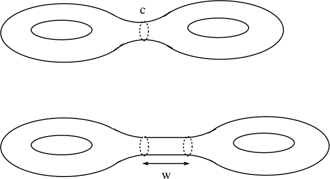
Figure 1: Grafting along a closed simple geodesic $c$ with weight $w$ on a genus 2 surface.

In the construction of (2+1)-spacetimes via grafting, the grafting procedure is applied to each two-surface $U_{\Lambda,S}(T)/\Gamma$ in (105). The construction is performed on their universal covers, i. e. the constant cosmological time surfaces $U_{\Lambda,S}(T)$, which are identified with copies of hyperbolic space via (96) and foliate the static domains $U_{\Lambda,S}\subset\mathbb{X}_{\Lambda,S}$ as in (98). The first step in the grafting construction is to lift each geodesic $\eta_{i}$ in the multicurve (106) to a geodesic $c_{\eta_{i}}$ on the universal cover $\mathbb{H}^{2}_{k}$. By acting on these geodesics with the cocompact Fuchsian group $\Gamma$, one obtains a $\Gamma$-invariant multicurve on $\mathbb{H}^{2}_{k}$

$$G^{\mathbb{H}^{2}_{k}}=\{(vc_{\eta_{i}},w_{i})\;|\;i\in I,v\in\Gamma\},$$ (107)

i. e. a set of non-intersecting geodesics on $\mathbb{H}^{2}_{k}$ with associated weights $w_{i}>0$, which are mapped into each other by the elements of $\Gamma$. Via the maps $\Phi^{\Lambda,S}_{T}:\mathbb{H}^{2}\rightarrow U_{\Lambda,S}(T)\subset\mathbb{X}_{\Lambda,S}$ in (96), which identify hyperbolic space with the constant cosmological time surfaces $U_{\Lambda,S}(T)$, one then obtains a $\Gamma$-invariant set of non-intersecting geodesics on each surface $U_{\Lambda,S}(T)$.

Grafting along the multicurve (106) assigns to each surface $U_{\Lambda,S}(T)$ a deformed surface $U^{G}_{\Lambda,S}(T)$ constructed as follows. One selects a basepoint $q_{0}\in\mathbb{H}^{2}$ outside of the geodesics in the multicurve (106) and considers the images $\Phi^{\Lambda,S}_{T}(q_{0})$ on the surfaces $U_{\Lambda,S}(T)$. One then cuts each surface $U_{\Lambda,S}(T)$ along the images $\Phi_{T}^{\Lambda,S}(vc_{\eta_{i}})$, $i\in I$, $v\in\Gamma$ of the geodesics in the multicurve (107) on $U_{\Lambda,S}(T)$. The resulting pieces which do not contain the images of the basepoint are then shifted away from the basepoint in the direction determined by the geodesics’ unit translation vectors and by a distance given by the geodesic’s weight. Finally, one inserts strips, which connect the shifted pieces of each constant cosmological time surface $U_{\Lambda,S}(T)$, and thus obtains a connected deformed surface $U^{G}_{\Lambda,S}(T)$

The union of these deformed surfaces for all values of the cosmological time $T$ then forms a simply connected regular domain in $\mathbb{X}_{\Lambda,S}$

$$U_{\Lambda,S}^{G}=\begin{cases}\bigcup_{T\in(0,\infty)}U_{0,L}^{G}(T)&\Lambda=0,\;\text{Lorentzian}\\ \bigcup_{T\in(0,\pi/\sqrt{\Lambda})}U_{\Lambda,L}^{G}(T)&\Lambda>0,\;\text{Lorentzian}\\ \bigcup_{T\in(0,\infty)}U_{\Lambda,L}^{G}(T)&\Lambda<0,\;\text{Lorentzian }\\ \bigcup_{T\in(0,\infty)}U_{\Lambda,E}^{G}(T)&\Lambda<0,\;\text{Euclidean}.\end{cases}$$ (108)

Under the grafting construction, the initial singularity of the static domains $U_{\Lambda,S}$ is mapped to a graph in $\mathbb{X}_{\Lambda,S}$. It is shown in [21, 22] that the deformed surfaces $U_{\Lambda,S}^{G}(T)$ are surfaces of constant geodesic distance $T$ from this graph and therefore again surfaces of constant cosmological time $T$.

It is discussed in [21, 22] that the cocompact Fuchsian group $\Gamma$ acts on the grafted domain $U_{\Lambda,S}^{G}(T)$ via a group homomorphism $h_{\Lambda,S}^{G}:\Gamma\rightarrow\text{Isom}(\mathbb{X}_{\Lambda,S})$. This action is free and properly discontinuous and preserves each surface $U_{\Lambda,S}^{G}(T)$. Hence, by taking the quotient $U_{\Lambda,S}^{G}(T)/h_{\Lambda,S}^{G}(\Gamma)$ of the deformed constant cosmological time surfaces by this action of $\Gamma$ one obtains a two-surface of genus $g$. The grafted spacetimes $M_{\Lambda,S}^{\Gamma,G}$ associated to the cocompact Fuchsian group $\Gamma$ and the multicurve (106) on $\mathbb{H}^{2}_{k}/\Gamma$ are then given as the union of these surfaces for all values of the cosmological time or, equivalently, as the quotient of the regular domains $U_{\Lambda,S}^{G}$ by this action of $\Gamma$

$$M_{\Lambda,S}^{\Gamma,G}=U_{\Lambda,S}^{G}/h^{G}_{\Lambda,S}(\Gamma)=\bigcup_{T}U_{\Lambda,S}^{G}(T)/h_{\Lambda,S}^{G}(\Gamma).$$ (109)

The procedure is most easily visualised in Lorentzian (2+1)-gravity with vanishing cosmological constant, where the surfaces of constant cosmological time are the hyperboloids $\mathbb{H}^{2}_{1/T^{2}}$ which foliate the interior of the forward lightcone. Geodesics on the hyperboloids $\mathbb{H}^{2}_{1/T^{2}}$ are given as the intersection of $\mathbb{H}^{2}_{1/T^{2}}$ with planes through the origin, whose unit normal vector is the unit translation vector of the geodesic given in (49). Cutting each surface $U_{0,L}(T)$ along these geodesics therefore amounts to cutting the interior of the forward lightcone along the associated planes. The resulting pieces are then shifted away from the basepoint in the direction of the plane’s normal vector by a distance given by the weight of the associated geodesic as shown in Fig.2.

hyper.eps

Figure 2: Grafting along a geodesic with weight $w$ in hyperbolic space.

The strips connecting the different pieces of a surface $U_{0,L}(T)$ are obtained by connecting the points the different pieces of $U_{0,L}(T)$ which correspond to a single point on a geodesic by straight lines.

For the other model spacetimes the construction is similar but its description is more involved. As we will not need the details of the construction, we refer the reader to the papers [21, 22], which give an explicit parametrisation of the resulting surfaces and relate these surfaces for different values of the cosmological constant. In the following, we will only make use of a formula for the translation of the images $\Phi^{\Lambda,S}_{T}(x)\in U_{\Lambda,S}(T)$ of points outside of the geodesics in the multicurve (107). The relative shift of such points under the grafting construction is determined by their position relative to the geodesics in (107) and given by a map $B_{G,\Lambda,S}:\mathbb{H}^{2}\times\mathbb{H}^{2}\rightarrow\text{Isom}(\mathbb{X}_{\Lambda,S})$. To determine the value of $B_{G,\Lambda,S}(p,q)$ for two points $p,q\in\mathbb{H}^{2}$ outside the geodesics in (107), one connects them with a geodesic $a_{pq}$ on $\mathbb{H}^{2}$ oriented towards $q$. One then determines the geodesics in the multicurve (107) which intersect this geodesic as well as the associated oriented intersection numbers. It is shown in [21, 22], see in particular Sect. 4.2.1, 4.4.1, 4.6.1 and 4.7.2, that if these geodesics are labelled by $c_{i}$, $i=1,\ldots,m$, such that the intersection point of $a_{pq}$ with $c_{i}$ occurs before the one with $c_{j}$ for $i<j$ and if $\epsilon_{i}$ are the associated oriented intersection numbers with the convention $\epsilon_{i}=1$ if $c_{i}$ crosses $a_{pq}$ from the left to the right, then the relative shift $B_{G,\Lambda,S}(p,q)$ is given by

$$B_{G,0,L}(p,q)=\sum_{i=1}^{n}m\epsilon_{i}w_{i}\hat{\mbox{\boldmath$n$}}_{i}\;\in\mathbb{R}^{3}\subset PSU(1,1)\ltimes\mathbb{R}^{3}$$ (110)

$$B_{G,\Lambda>0,L}(p,q)=(B^{+}_{G,\Lambda>0,L}(p,q),B^{-}_{G,\Lambda>0,L}(p,q))\in PSU(1,1)\times PSU(1,1)$$

$$\qquad\qquad\qquad\qquad B^{\pm}_{G,\Lambda>0,L}(p,q)=e^{\pm\sqrt{\Lambda}{\epsilon_{1}w_{1}}\hat{n}_{1}^{a}J_{a}^{L}}e^{{\pm\sqrt{\Lambda}\epsilon_{2}w_{2}}\hat{n}_{2}^{a}J_{a}^{L}}\cdots e^{\pm{\sqrt{\Lambda}\epsilon_{n}w_{n}}\hat{n}_{m}^{a}J_{a}^{L}}$$

$$B_{G,\Lambda<0,S}(p,q)=B_{G,\Lambda<0,E}(p,q)=e^{{i\sqrt{|\Lambda|}\epsilon_{1}w_{1}}\hat{n}_{1}^{a}J_{a}^{L}}e^{i\sqrt{|\Lambda|}\epsilon_{2}w_{2}\hat{n}_{2}^{a}J_{a}^{L}}\cdots e^{{i\sqrt{|\Lambda|}\epsilon_{n}w_{n}}\hat{n}_{m}^{a}J_{a}^{L}}\in SL(2,\mathbb{C})/\mathbb{Z}_{2},$$

where $w_{i}$ is the weight of the geodesic $c_{i}$ and $\hat{\mbox{\boldmath$n$}}_{i}$ its unit translation vector as defined in (49). It is shown in [21, 22] that map $B_{G,\Lambda,S}:\mathbb{H}^{2}\times\mathbb{H}^{2}\rightarrow\text{Isom}(\mathbb{X}_{\Lambda,S})$ satisfies the identities

$$B_{G,\Lambda,S}(p,q)\cdot B_{G,\Lambda,S}(q,r)=B_{G,\Lambda,S}(p,r) \forall p,q,r\in\mathbb{H}^{2}$$ (111)

$$B_{G,\Lambda,S}(vp,vq)=\i_{\Lambda,S}(v)\cdot B_{G,\Lambda,S}(p,q)\cdot\i_{\Lambda,S}(v)^{-1} \forall p,q\in\mathbb{H}^{2},\,v\in PSU(1,1),$$

which reflect the geometrical properties of the grafting procedure. This allows one to define a group homomorphism $h^{G}_{\Lambda,S}:\Gamma\rightarrow\text{Isom}(\mathbb{X}_{\Lambda,S})$ from the cocompact Fuchsian group $\Gamma$ into the isometry group of the model spacetime by setting

$$h_{\Lambda,S}^{G}(v)=B_{G,\Lambda,S}(q_{0},vq_{0})\cdot\i_{\Lambda,S}(v)\qquad\forall v\in\Gamma,$$ (112)

where $\i_{\Lambda,S}:PSU(1,1)\rightarrow\text{Isom}(\mathbb{X}_{\Lambda,S})$ is the canonical embedding of $PSU(1,1)$ into the isometry group of the model spacetime given by (38) and $q_{0}\in\mathbb{H}^{2}$ the basepoint. It is discussed in [21, 22] that this group homomorphism defines a free and properly discontinuous action of the group $\Gamma$ on the grafted domains $U^{G}_{\Lambda,S}$ which maps each surface $U^{G}_{\Lambda,S}(T)$ to itself. Furthermore, for any two points $\Phi^{\Lambda}_{T}(x)$, $\Phi^{\Lambda}_{T}(x^{\prime})\in U_{\Lambda,S}(T)$ outside the geodesics which are related by the canonical action (97) of an element $v\in\Gamma$, the corresponding points on the grafted surface $U_{\Lambda,S}^{G}(T)$ are related by the action of $v$ via (112)

$$\Phi_{\Lambda,S}^{T}(x^{\prime})=\i_{\Lambda,S}(v)\cdot\Phi_{\Lambda,S}^{T}(x)$$ (113)

$$\Rightarrow\quad B_{G,\Lambda,S}(q_{0},x^{\prime})\Phi_{\Lambda,S}^{T}(x^{\prime})=h_{\Lambda,S}^{G}(v)\cdot B_{G,\Lambda,S}(q_{0},x)\Phi_{\Lambda,S}^{T}(x).$$

The quotient (109) of the domains $U^{G}_{\Lambda,S}\subset\mathbb{X}_{\Lambda,S}$ by this action of $\Gamma$ is therefore well-defined and gives rise to a spacetime of topology $\mathbb{R}\times S_{g}$.

4 (2+1)-dimensional gravity: the Chern-Simons formulation

4.1 (2+1)-dimensional gravity as a Chern-Simons gauge theory

The absence of local gravitational degrees of freedom in (2+1)-dimensional gravity allows one to formulate the theory as a Chern-Simons gauge theory [3, 4]. The Chern-Simons formulation of (2+1)-dimensional gravity is derived from Cartan’s description, in which a spacetime manifold $M$ is characterised in terms of a dreibein of one forms $e_{a}$, $a=0,1,2$, and spin connection one-forms $\omega_{a}$, $a=0,1,2$, on $M$. The metric on $M$ is given by the dreibein

$$g=\eta_{S}^{ab}e_{a}\otimes e_{b},$$ (114)

where $\eta^{ab}_{S}$ denotes the Minkowski metric (1) or the Euclidean metric (2)., while the one-forms $\omega_{a}$ are the coefficients of the spin connection $\omega=\omega^{a}J^{S}_{a}$. Einstein’s equations of motion then take the form of the requirements of vanishing torsion and constant curvature

$$T^{a}=de^{a}+\epsilon^{a}_{\;\;bc}\omega^{b}e^{c}=0\qquad F_{\omega}^{a}=d\omega^{a}+\frac{1}{2}\epsilon^{a}_{\;\;bc}\omega^{b}\wedge\omega^{c}=-\tfrac{\Lambda}{2}\epsilon^{a}_{\;\;bc}e^{b}\wedge e^{c}.$$ (115)

To obtain the Chern-Simons formulation of (2+1)-dimensional gravity, one combines dreibein and spin connection into the Cartan connection [32] or Chern-Simons gauge field

$$A=\omega^{a}J^{S}_{a}+e^{a}P^{S}_{a},$$ (116)

where $J_{a}^{S}$, $P_{a}^{S}$, $a=0,1,2$, denote the generators of the six-dimensional Lie algebras $\mathfrak{h}_{\Lambda,S}$ with bracket (3),(4). Hence, depending on the signature and the cosmological constant, the Chern-Simons gauge field is a one-form on $M$ with values in the Lie algebra $\mathfrak{h}_{\Lambda,S}$. The choice of the Lie algebra determines the gauge group of the associated Chern-Simons theory up to coverings, and in the following, we will take the isometry groups $\text{Isom}(\mathbb{X}_{\Lambda,S})$ of the associated model spacetimes as the gauge groups.

When expressed in terms of the one-form (116), the Einstein-Hilbert action in Cartan’s formulation of the theory takes the form of a Chern-Simons action

$$S_{CS}[A]=\int_{M}\langle A\wedge dA+\tfrac{2}{3}A\wedge A\wedge A\rangle,$$ (117)

where $\langle\,,\,\rangle$ is an $\mathrm{Ad}$-invariant, non-degenerate bilinear form on the Lie algebra $\mathfrak{h}_{\Lambda,S}$ given by

$$\langle J_{a}^{S},P^{S}_{b}\rangle=\eta^{S}_{ab}\qquad\langle J^{S}_{a},J^{S}_{b}\rangle=\langle P^{S}_{a},P^{S}_{b}\rangle=0.$$ (118)

The equations of motion derived from (117) are a flatness condition on the gauge field

$$F=dA+A\wedge A=0,$$ (119)

which combines the requirements (115) of vanishing torsion and constant curvature

$$F=T^{a}P^{S}_{a}+(F_{\omega}^{a}+\tfrac{\Lambda}{2}\epsilon^{a}_{\;\;bc}e^{b}\wedge e^{c})\,J^{S}_{a}.$$ (120)

The Chern-Simons action (117) is invariant under Chern-Simons gauge transformations

$$A\mapsto\gamma A\gamma^{-1}+\gamma d\gamma^{-1}\qquad\gamma:M\rightarrow\text{Isom}(\mathbb{X}_{\Lambda,S}).$$ (121)

It has been shown by Witten [4] that infinitesimal Chern-Simons gauge transformations are on-shell equivalent to infinitesimal diffeomorphisms. The space of metrics solving Einsteins’s equation modulo infinitesimally generated diffeomorphisms is therefore isomorphic to the space of flat Chern-Simons gauge fields modulo infinitesimally generated Chern-Simons gauge transformations.

Note, however, that some caution should be applied when identifying the phase space of (2+1)-dimensional gravity in its geometrical formulation with the phase space of the associated Chern-Simons theory. First, the equivalence between diffeomorphisms and Chern-Simons gauge transformations does not hold for large diffeomorphisms, which are not infinitesimally generated, and for the large gauge transformations arising in Chern-Simons theory with non-simply connected gauge groups. Second, in order to define a metric of Lorentzian or Euclidean signature via (114), the dreibein $e_{a}$ has to be non-degenerate, which is not required in the Chern-Simons formalism. It is discussed in [33] for the Lorentzian case with vanishing cosmological constant and spacetimes containing particles that this leads to differences in the global structure of the phase spaces. A similar result for a spacetime with three particles is derived in [22], Sect. 4.9, where it is argued that such problems arise generically when the spacetime is of topology $\mathbb{R}\times S$, where $S$ is a non-compact two-surface. However, as this paper restricts attention to spacetimes with compact spatial surfaces and is mainly concerned with the local properties of the phase space, we will not address these issues in the following.

On the spacetime manifolds of topology $M\cong\mathbb{R}\times S_{g}$ considered in this paper, it is possible to give a Hamiltonian formulation of the theory. For this, one introduces coordinates $x^{0},x^{1},x^{2}$ on $M\approx\mathbb{R}\times S_{g}$ such that $x^{0}$ parametrises $\mathbb{R}$ and $x^{1},x^{2}$ are coordinates on $S_{g}$ and splits the gauge field (116) as

$$A=A_{0}dx^{0}+A_{S},$$ (122)

where $A_{0}:\mathbb{R}\times S_{g}\rightarrow\mathfrak{h}_{\Lambda,S}$ is a function with values in the Lie algebras $\mathfrak{h}_{\Lambda,S}$ and $A_{S}$ a gauge field on $S_{g}$. The Chern-Simons action (117)on $M$ then takes the form

$$S[A_{S},A_{0}]=\int_{\mathbb{R}}dx^{0}\int_{S_{g}}\tfrac{1}{2}\langle\partial_{0}A_{S}\wedge A_{S}\rangle+\langle A_{0}\,,\,F_{S}\rangle,$$ (123)

where $F_{S}$ is the curvature of the spatial gauge field $A_{S}$

$$F_{S}=d_{S}A_{S}+A_{S}\wedge A_{S}$$ (124)

with $d_{S}$ denoting differentiation on the surface $S_{g}$. The function $A_{0}$ plays the role of a Lagrange multiplier. Varying it leads to the flatness constraint

$$F_{S}=0,$$ (125)

while variation of $A_{S}$ results in the evolution equation

$$\partial_{0}A_{S}=d_{S}A_{0}+[A_{S},A_{0}].$$ (126)

The phase space of the theory is therefore the moduli space $\mathcal{M}_{g}^{\text{Isom}(\mathbb{X}_{\Lambda,S})}$ of flat $\text{Isom}(\mathbb{X}_{\Lambda,S})$-connections $A_{S}$ modulo gauge transformations on the spatial surface $S_{g}$.

4.2 Trivialisation and holonomies

As discussed in Sect. 3, the absence of local gravitational degrees of freedom in (2+1)-dimensional gravity implies that each (2+1)-spacetime is locally isometric to one of the model spacetimes $\mathbb{X}_{\Lambda,S}$. In the Chern-Simons formalism, this absence of local degrees of freedom manifests itself in the fact that gauge fields solving the equations of motions are flat and can be trivialised, i. e. written as pure gauge on any simply connected region $R\subset\mathbb{R}\times S_{g}$

$$A=\gamma d\gamma^{-1}\qquad\gamma:R\rightarrow\text{Isom}(\mathbb{X}_{\Lambda,S}).$$ (127)

Given a function $\gamma:R\rightarrow\text{Isom}(\mathbb{X}_{\Lambda,S})$ which trivialises a flat gauge field $A$ on $R$, the associated functions $\gamma(x^{0},\cdot)$ trivialise the corresponding flat spatial gauge fields $A_{s}$ for all values of $x^{0}$

$$A_{S}(x^{0},\cdot)=\gamma(x^{0},\cdot)d_{S}\gamma^{-1}(x^{0},\cdot).$$ (128)

To simplify notation, we will often neglect the dependence on the parameter $x^{0}$ in the following and denote this function also by $\gamma$.

A maximal simply connected region in $\mathbb{R}\times S_{g}$ is obtained by cutting the spatial surface $S_{g}$ along a set of generators of the fundamental group $\pi_{1}(S_{g})$ as in Fig. 3.

cutgr.eps

Figure 3: Cutting the surface $S_{g}$ along the generators of $\pi_{1}(S_{g})$

As discussed in Sect. 2.2, the fundamental group of a genus $g$ surface $S_{g}$ is isomorphic to a cocompact Fuchsian group with $2g$ generators, which are subject to a single defining relation

$$\pi_{1}(S_{g})=\langle a_{1},b_{1},\ldots,a_{g},b_{g}\,;\,[b_{g},a_{g}^{-1}]\cdots[b_{1},a_{1}^{-1}]=1\rangle\qquad[b_{i},a_{i}^{-1}]=b_{i}\circ a_{i}^{-1}\circ b_{i}^{-1}\circ a_{i}.$$ (129)

Throughout the paper, we work with a fixed system of generators $a_{i},b_{i}$, $i=1,\ldots,g$, which are the homotopy equivalence classes of two loops around each handle and based at a point $p\in S_{g}$ as shown in Fig. 4.

pi1gr.eps

Figure 4: Generators and dual generators of the fundamental group $\pi_{1}(S_{g})$

Cutting the surface along each of the curves representing these generators results in a $4g$-gon $P_{g}$ pictured in Fig. 5.

poly1.eps

Figure 5: The polygon $P_{g}$

As discussed by Alekseev and Malkin [13], a function $\gamma:P_{g}\rightarrow\text{Isom}(\mathbb{X}_{\Lambda,S})$ on $P_{g}$ defines a flat gauge field on $S_{g}$ if and only if it satisfies an overlap condition relating its value on the two sides which correspond to a given generator of the fundamental group. For any $y\in\{a_{1},b_{1},\ldots,a_{g},b_{g}\}$, $y^{\prime}\in\{a^{\prime}_{1},b^{\prime}_{1},\ldots,a^{\prime}_{g},b^{\prime}_{g}\}$ one must have

$$A_{S}|_{y^{\prime}}=\gamma d_{S}\gamma^{-1}|_{y^{\prime}}=\gamma d_{S}\gamma^{-1}|_{y}=A_{S}|_{y},$$ (130)

which is the case if and only if there exist constant elements $N_{Y}\in\text{Isom}(\mathbb{X}_{\Lambda,S})$ such that

$$\gamma^{-1}|_{y^{\prime}}=N_{Y}\gamma^{-1}|_{y}.$$ (131)

The elements $N_{Y}$, $Y\in\{A_{1},B_{1},\ldots,A_{g},B_{g}\}$ are the Chern-Simons analogue of the group isomorphisms (112) in the geometrical formulation. They contain all information about the physical state and are closely related to the holonomies $A_{i},B_{i}$ along the generators $a_{i},b_{i}$ of the fundamental group. These holonomies are given by the value of the trivialising function on the corners of the polygon $P_{g}$ [13]

$${A_{i}}\!=\!\gamma(p_{4i-3})\gamma(p_{4i-4})^{-1}\!\!=\!\gamma(p_{4i-2})\gamma(p_{4i-1})^{-1}\;\;{B_{i}}\!=\!\gamma(p_{4i-3})\gamma(p_{4i-2})^{-1}\!\!\!=\gamma(p_{4i})\gamma(p_{4i-1})^{-1}\!\!\!\!,$$ (132)

and satisfy a single relation arising from the defining relation of the fundamental group $\pi_{1}(S_{g})$

$$[B_{g},A_{g}^{-1}]\cdots[B_{1},A_{1}^{-1}]\approx 1\qquad[B_{i},A_{i}^{-1}]=B_{i}\cdot{A_{i}}^{-1}\cdot{B_{i}}^{-1}\cdot{A_{i}}.$$ (133)

Via the overlap condition (130), one can relate the value of the trivialising function $\gamma$ at the corners of the polygon $P_{g}$ to its value at a given corner $p_{0}$

$$\gamma^{-1}(p_{4i})=N_{H_{i}}N_{H_{i-1}}\cdots N_{H_{1}}\gamma^{-1}(p_{0})=\gamma^{-1}(p_{0})H_{1}^{-1}\cdots H_{i-1}^{-1}H_{i}^{-1}$$ (134)

$$\gamma^{-1}(p_{4i+1})=N_{A_{i+1}}^{-1}N_{B_{i+1}}^{-1}N_{A_{i+1}}N_{H_{i}}\cdots N_{H_{1}}\gamma^{-1}(p_{0})=\gamma^{-1}(p_{0})H_{1}^{-1}\cdots H_{i-1}^{-1}H_{i}^{-1}A_{i+1}^{-1}$$

$$\gamma^{-1}(p_{4i+2})=N_{B_{i+1}}^{-1}N_{A_{i+1}}N_{H_{i}}\cdots N_{H_{1}}\gamma^{-1}(p_{0})=\gamma^{-1}(p_{0})H_{1}^{-1}\cdots H_{i-1}^{-1}H_{i}^{-1}A_{i+1}^{-1}B_{i+1}$$

$$\gamma^{-1}(p_{4i+3})=N_{A_{i+1}}N_{H_{i}}\cdots N_{H_{1}}\gamma^{-1}(p_{0})=\gamma^{-1}(p_{0})H_{1}^{-1}\cdots H_{i-1}^{-1}H_{i}^{-1}A_{i+1}^{-1}B_{i+1}A_{i+1}$$

$$H_{i}=[B_{i},A_{i}^{-1}]\qquad N_{H_{i}}=[N_{B_{i}},N_{A_{i}}^{-1}],$$

which allows one to express the holonomies $A_{i},B_{i}$ along the generators $a_{i},b_{i}\in\pi_{1}(S_{g})$ in terms of the Poincaré elements $N_{A_{i}},N_{B_{i}}$ in the overlap condition (130) and vice versa

$$A_{i}=\gamma(p_{0})N_{H_{1}}^{-1}\cdots N_{H_{i-1}}^{-1}N_{H_{i}}^{-1}\cdot N_{{B_{i}}}\cdot N_{H_{i-1}}\cdots N_{H_{1}}\gamma^{-1}(p_{0})$$ (135)

$${B_{i}}=\gamma(p_{0})N_{H_{1}}^{-1}\cdots N_{H_{i-1}}^{-1}N_{H_{i}}^{-1}\cdot N_{{A_{i}}}\cdot N_{H_{i-1}}\cdots N_{H_{1}}\gamma^{-1}(p_{0})$$

$$N_{A_{i}}\!\!=\!\!\gamma^{-1}(p_{0})H_{1}^{-1}\!\!\!\!\!\cdots\!H_{i-1}^{-1}H_{i}^{-1}{B_{i}}H_{i-1}\!\cdots\!H_{1}\gamma(p_{0})$$ (136)

$$N_{B_{i}}\!\!=\!\!\gamma^{-1}(p_{0})H_{1}^{-1}\!\!\!\!\!\cdots\!H_{i-1}^{-1}H_{i}^{-1}{A_{i}}H_{i-1}\!\cdots\!H_{1}\gamma(p_{0}).$$

Up to conjugation with the value $\gamma(p_{0})$ of the trivialising function at the basepoint, the expressions (135) and (136) relating the holonomies ${A_{i}},{B_{i}}$ and the group elements $N_{A_{i}},N_{B_{i}}$ are of the same form. This reflects the fact that, up to conjugation with $\gamma(p_{0})$, the elements $N_{A_{i}},N_{B_{i}}$ are the holonomies along another system of generators ${\overline{a}}_{i},{\overline{b}}_{i}\in\pi_{1}(S_{g})$ pictured in Fig. 4 and given by

$${\overline{a}}_{i}\!=\!h_{1}^{-1}\circ...\circ h_{i}^{-1}\circ b_{i}\circ h_{i-1}\circ...\circ h_{1}\qquad{\overline{b}}_{i}\!=\!h_{1}^{-1}\circ...\circ h_{i}^{-1}\circ a_{i}\circ h_{i-1}\circ...\circ h_{1}.$$ (137)

These generators are investigated in detail in [34], where it is shown that their representatives can be viewed as a dual graph for the curves representing $a_{i},b_{i}\in\pi_{1}(S_{g})$ and that they can be used to determine the intersection points of a general embedded curve on $S_{g}$ with the generators $a_{i},b_{i}$. In the following we will therefore refer to the generators ${\overline{a}}_{i},{\overline{b}}_{i}$ as the dual generators.

As the elements $N_{A_{i}},N_{B_{i}}\in\text{Isom}(\mathbb{X}_{\Lambda,S})$ in the overlap condition or, equivalently, the holonomies ${A_{i}},{B_{i}}\in\text{Isom}(\mathbb{X}_{\Lambda,S})$ contain all information about the physical state, they can be used to parametrise the phase space of the theory. Taking into account that these variables are subject to a constraint (133) and that gauge transformations on the surface $S_{g}$ act on the holonomies $A_{i},B_{i}$ by simultaneous conjugation, one finds that the moduli space of flat $\text{Isom}(\mathbb{X}_{\Lambda,S})$-connections on $S_{g}$ is given as the quotient

$$\mathcal{M}_{g}^{\text{Isom}(\mathbb{X}_{\Lambda,S})}\!\!\!\!\!\!\!\!=\{(A_{1},B_{1},\ldots,A_{g},B_{g})\in\text{Isom}(\mathbb{X}_{\Lambda,S})^{2g}\;|\;[B_{g},A_{g}^{-1}]\cdots[B_{1},A_{1}^{-1}]=1\}/\text{Isom}(\mathbb{X}_{\Lambda,S}).$$ (138)

4.3 Phase space and Poisson structure

The advantage of the Chern-Simons formulation of (2+1)-dimensional gravity is that it allows one to give a rather simple description of the Poisson structure on the phase space, which is based on its parametrisation (138) in terms of the holonomies along a set of generators $a_{i},b_{i}\in\pi_{1}(S_{g})$ [13, 12]. In the following we will use the formalism by Fock and Rosly [12], which is defined for Chern-Simons theory with a general gauge group $H$ and parametrises the Poisson structure on the moduli space $\mathcal{M}_{g}^{H}$ in terms of an auxiliary Poisson structure on the manifold $H^{2g}$. The description is summarised in the following theorem.

Theorem 4.1.

(Fock,Rosly [12])

Consider Chern-Simons theory with gauge group $H$ on a manifold $\mathbb{R}\times S_{g}$. Denote by $T_{a}$, $a=1,\ldots,\text{dim}\;H$, a basis of the Lie algebra $\mathfrak{h}=\text{Lie}\;H$ and by $t_{ab}$ the matrix representing the $\mathrm{Ad}$-invariant symmetric bilinear form in the Chern-Simons action (117) with respect to this basis

$$t_{ab}=\langle T_{a},T_{b}\rangle\qquad t^{ab}t_{bc}=\delta^{a}_{c}.$$ (139)

Let $r=r^{ab}T_{a}\otimes T_{b}$ be a classical $r$-matrix for the gauge group $H$, i. e. an element $r\in\mathfrak{h}\otimes\mathfrak{h}$ which satisfies the classical Yang Baxter equation (CYBE)

$$[[r,r]]=[r_{12},r_{13}]+[r_{12},r_{23}]+[r_{13},r_{23}]=0$$ (140)

$$r_{12}=r^{ab}T_{a}\otimes T_{b}\otimes 1,\;r_{13}=r^{ab}T_{a}\otimes 1\otimes T_{b},r_{23}=r^{ab}1\otimes T_{a}\otimes T_{b},$$

and whose symmetric part is dual to the bilinear form (139)

$$r=r_{(s)}+r_{(a)}\qquad r_{(a)}=\tfrac{1}{2}(r^{ab}-r^{ba})T_{a}\otimes T_{b}\;,\quad r_{(s)}=\tfrac{1}{2}(r^{ab}+r^{ba})T_{a}\otimes T_{b}=\tfrac{1}{2}t^{ab}T_{a}\otimes T_{b}.$$ (141)

Consider the manifold $H^{2g}$, where the different copies of $H$ are identified with the holonomies ${A_{i}},{B_{i}}\in H$ along a set of generators of the fundamental group $\pi_{1}(S_{g})$ and denote by $R_{a}^{X}$, $L_{a}^{X}$, $X\in\{A_{1},B_{1},\ldots,A_{g},B_{g}\}$ the left-and right-invariant vector fields associated to a basis of $\mathfrak{h}$ and the different components of $H^{2g}$

$$L_{a}^{X}f(A_{1},...,B_{g})=\frac{d}{dt}|_{t=0}f(...,e^{-tT_{a}}\cdot X,...)\quad R_{a}^{X}f(A_{1},...,B_{g})=\frac{d}{dt}|_{t=0}f(...,X\cdot e^{tT_{a}},...).$$ (142)

Then, the bivector $B\in\text{Vec}(H)\otimes\text{Vec}(H)$

$$B= r^{ab}_{(a)}\!\!\left(\!\sum_{j=1}^{g}R^{{A_{j}}}_{a}\!+\!L^{{A_{j}}}_{a}\!+\!R^{{B_{j}}}_{a}\!+\!L^{{B_{j}}}_{a}\right)\!\!\otimes\!\!\left(\sum_{j=1}^{g}R^{{A_{j}}}_{b}\!+\!L^{{A_{j}}}_{b}\!+\!R^{{B_{j}}}_{b}\!+\!L^{{B_{j}}}_{b}\right)$$

$$+ \tfrac{1}{2}t^{ab}\!\!\!\!\sum_{i,j=1,\;i<j}^{g}(R^{{A_{i}}}_{a}\!+\!L^{{A_{i}}}_{a}\!+\!R^{{B_{i}}}_{a}\!+\!L^{{B_{i}}}_{a})\wedge(R^{{A_{j}}}_{b}\!+\!L^{{A_{j}}}_{b}\!+\!R^{{B_{j}}}_{b}\!+\!L^{{B_{j}}}_{b})$$

$$+ \tfrac{1}{2}t^{ab}\sum_{i=1}^{g}R^{A_{i}}_{a}\wedge(R^{B_{i}}_{b}+L^{A_{i}}_{b}+L^{B_{i}}_{b})+R^{B_{i}}_{a}\wedge(L^{A_{i}}_{b}+L^{B_{i}}_{b})+L^{A_{i}}_{a}\wedge L^{B_{i}}_{b},$$ (143)

defines a Poisson structure on $H^{2g}$. After imposing the constraint (133) and dividing by the associated gauge transformations, which act by simultaneous conjugation of all components with $H$, this Poisson structure agrees with the canonical Poisson structure on the moduli space

$$\mathcal{M}^{H}_{g}=\{(A_{1},B_{1},\ldots,A_{g},B_{g})\in H^{2g}\;|\;[B_{g},A_{g}^{-1}]\cdots[B_{1},A_{1}^{-1}]=1\}/H.$$ (144)

In Fock and Rosly’s formalism, physical observables are given by functions on the manifold $H^{2g}$ which are invariant under simultaneous conjugation of all components with the gauge group $H$. Note that the Poisson bracket of such observables with a general function $g\in\mathcal{C}^{\infty}(H^{2g})$ does not depend on the particular choice of the classical $r$-matrix but only on the matrix $t^{ab}$ representing the $\mathrm{Ad}$-invariant, symmetric bilinear form in the Chern-Simons action. As the component of the bivector (4.1) which depends on the antisymmetric component $r_{(a)}$ is proportional to terms of the form $\sum_{i=1}^{g}R^{A_{i}}_{a}+L^{A_{i}}_{a}+R^{B_{i}}_{a}+L_{B_{i}}^{a}$, this contribution vanishes if one of the function is invariant under simultaneous conjugation of its arguments with $H$.

A particular set of physical observables, in the following referred to as Wilson loop observables, are conjugation invariant functions of the holonomies along closed curves on $S_{g}$. As the equations of motion are a flatness condition on the gauge field, these observables do not depend on the curve itself but only on its homotopy equivalence class in $\pi_{1}(S_{g})$ and are invariant under a change of the basepoint. In Fock and Rosly’s formalism, these observables are described by expressing the holonomy along an element $\eta\in\pi_{1}(S_{g})$ as a product in the holonomies along the generators $a_{i},b_{i}\in\pi_{1}(S_{g})$

$$\eta=x_{r}^{\alpha_{r}}\cdots x_{1}^{\alpha_{1}}\,,\;x_{k}\in\{a_{1},\ldots,b_{g}\},\;\alpha_{k}\in\{\pm 1\}\quad\Rightarrow\quad H_{\eta}=X_{r}^{\alpha_{r}}\cdots X_{1}^{\alpha_{1}}.$$ (145)

The Wilson loop observable $f_{\eta}\in\mathcal{C}^{\infty}(H^{2g})$ associated to $\eta\in\pi_{1}(S_{g})$ and a general conjugation invariant function $f\in\mathcal{C}^{\infty}(H)$ on the gauge group is then given by

$$f_{\eta}:(A_{1},\ldots,B_{g})\mapsto f(H_{\eta})$$ (146)

with $H_{\eta}$ given as a product in the elements ${A_{i}},{B_{i}}$ and their inverses as in (145). It follows directly that the Wilson loop observables are invariant under simultaneous conjugation of all holonomies $A_{i},B_{i}$ with elements of $H$ and satisfy

$$f_{\tau\circ\eta\circ\tau^{-1}}=f_{\eta}\qquad\forall\eta,\tau\in\pi_{1}(S_{g}).$$ (147)

In order to apply Fock and Rosly’s description [12] of phase space and Poisson structure to the Chern-Simons formulation of (2+1)-dimensional gravity, one needs classical $r$-matrices for the Lie algebras $\mathfrak{h}_{\Lambda,S}$ such that the symmetric components of these $r$-matrices agree with the $\mathrm{Ad}$-invariant, symmetric bilinear forms (118). For Lorentzian signature, such a classical $r$-matrix is given by

$$r=P^{L}_{a}\otimes J_{L}^{a}+n_{a}\epsilon^{abc}J^{L}_{b}\otimes J^{L}_{c}\$$ (148)

with a constant vector ${\mbox{\boldmath$n$}}=(n^{0},n^{1},n^{2})\in\mathbb{R}^{3}$ satisfying $\eta^{L}({\mbox{\boldmath$n$}},{\mbox{\boldmath$n$}})=\Lambda$. The corresponding $r$-matrix for the Euclidean case with $\Lambda<0$ has the form

$$r^{E}=P^{E}_{a}\otimes J_{E}^{a}+n_{a}\epsilon^{abc}J^{E}_{b}\otimes J^{E}_{c}$$ (149)

with a constant vector ${\mbox{\boldmath$n$}}=(n_{0},n_{1},n_{2})\in\mathbb{R}^{3}$ satisfying $\eta^{E}({\mbox{\boldmath$n$}},{\mbox{\boldmath$n$}})=|\Lambda|$. Note that the choice of the classical $r$-matrix and hence the Poisson structure (4.1) is not necessarily unique - for a list of classical $r$-matrices for the (2+1)-dimensional Poincaré algebra see [35]. However, in the following we will only consider Poisson brackets where at least one of the functions is a Wilson loop observable so that our results do not depend on this choice.

5 Trivialisation and embedding

As discussed in Sect. 3 and Sect. 4.2, the absence of local gravitational degrees of freedom manifests itself in the geometrical and the Chern-Simons description of (2+1)-spacetimes in, respectively, in the embedding of simply connected regions into the model spacetimes $\mathbb{X}_{\Lambda,S}$ and in the trivialisation of the Chern-Simons gauge field. In this section, we discuss the relation between these concepts and show how the embedding of spacetime regions can be constructed from the function trivialising the Chern-Simons gauge field.

We consider a simply connected region $R\subset\mathbb{R}\times S_{g}$ in the spacetime manifold with a metric $g$ and a flat Chern-Simons gauge field $A$, related to the metric via (114). We denote by ${\mbox{\boldmath$X$}}_{\Lambda,S}:R\rightarrow\mathbb{X}_{\Lambda,S}$ the embedding into the model spacetime $\mathbb{X}_{\Lambda,S}$ and by $\gamma:R\rightarrow\text{Isom}(\mathbb{X}_{\Lambda,S})$ a function which trivialises the gauge field as in (127). The decomposition (116) of the gauge field in terms of the generators $J_{a}^{S},P_{a}^{S}$ then implies that the dreibein $e_{a}$ and the spin connection $\omega_{a}$ are given by

$$e_{a}=\langle\gamma d\gamma^{-1},J^{S}_{a}\rangle\qquad\omega_{a}=\langle\gamma d\gamma^{-1},P_{a}^{S}\rangle,$$ (150)

where $J_{a}^{S}$, $P_{a}^{S}$ denote the generators of the Lie algebras (3), (4) and $\langle\,,\,\rangle$ the $\mathrm{Ad}$-invariant bilinear form (118) in the Chern-Simons action. The expression (114) for the metric in terms of the dreibein relating then implies that the metric $g$ on $R$ takes the form

$$g=\eta^{S}_{ab}e^{a}\otimes e^{b}=\eta_{S}^{ab}\langle\gamma d\gamma^{-1}\!\!\!,J_{a}^{S}\rangle\langle\gamma d\gamma^{-1}\!\!\!,J^{S}_{b}\rangle=-4\det(\eta_{S})\det(\langle\gamma d\gamma^{-1},J_{S}^{a}\rangle J_{a}^{S}).$$ (151)

On the other hand, the metric $g$ must agree with the pull-back of the metric in the model spacetime $\mathbb{X}_{\Lambda,S}$ via the embedding ${\mbox{\boldmath$X$}}_{\Lambda,S}$. To relate the trivialising function $\gamma:R\rightarrow\text{Isom}(\mathbb{X}_{\Lambda,S})$ to the embedding ${\mbox{\boldmath$X$}}_{\Lambda,S}:R\rightarrow\mathbb{X}_{\Lambda,S}$, one therefore has to construct a function $\Pi_{\Lambda,S}:\text{Isom}(\mathbb{X}_{\Lambda,S})\rightarrow\mathbb{X}_{\Lambda,S}$ from the isometry group into the model spacetime such that the pull-back of the metric in the model spacetime via $\Pi_{\Lambda,S}\circ\gamma^{-1}$ agrees with the metric (151)

$$d({\mbox{\boldmath$X$}}_{\Lambda,S}\circ\gamma^{-1})^{2}=\eta_{S}^{ab}\langle\gamma d\gamma^{-1}\!\!\!,J_{a}^{S}\rangle\langle\gamma d\gamma^{-1}\!\!\!,J^{S}_{b}\rangle.$$ (152)

Furthermore, as the embedding of the region $R$ into the model spacetime $\mathbb{X}_{\Lambda,S}$ is only defined up to a global action of the isometry group $\text{Isom}(\mathbb{X}_{\Lambda,S})$, two embeddings related by such an action of the isometry group should correspond to the same gauge field on $R$. This the case if and only if the action of $\text{Isom}(\mathbb{X}_{\Lambda,S})$ on $\mathbb{X}_{\Lambda,S}$ corresponds to left-multiplication of the trivialising function $\gamma^{-1}\mapsto N\gamma^{-1}$, $N\in\text{Isom}(\mathbb{X}_{\Lambda,S})$, i. e. if the function $\Pi_{\Lambda,S}:\text{Isom}(\mathbb{X}_{\Lambda,S})\rightarrow\mathbb{X}_{\Lambda,S}$ satisfies the condition

$$\Pi_{\Lambda,S}(N\gamma^{-1})=N\Pi_{\Lambda,S}(\gamma^{-1})\qquad\forall N\in\text{Isom}(\mathbb{X}_{\Lambda,S}).$$ (153)

This suggests that the functions $\Pi_{\Lambda,S}:\text{Isom}(\mathbb{X}_{\Lambda,S})\rightarrow\mathbb{X}_{\Lambda,S}$ should be defined as

$$\Pi_{0,L}(v,{\mbox{\boldmath$x$}})={\mbox{\boldmath$x$}} \forall(v,{\mbox{\boldmath$x$}})\in PSU(1,1)\ltimes\mathbb{R}^{3}$$ (154)

$$\Pi_{\Lambda>0,L}(v_{+},v_{-})=\tfrac{1}{\sqrt{\Lambda}}\,v_{+}v_{-}^{-1} \forall(v_{+},v_{-})\in PSU(1,1)\times PSU(1,1)$$

$$\Pi_{\Lambda<0,L}(v)=\tfrac{1}{\sqrt{|\Lambda|}}\,vv^{\circ} \forall v\in SL(2,\mathbb{C})/\mathbb{Z}_{2}$$

$$\Pi_{\Lambda<0,E}(v)=\tfrac{1}{\sqrt{|\Lambda|}}\,vv^{\dagger} \forall v\in SL(2,\mathbb{C})/\mathbb{Z}_{2},$$

since this ensures that identity (153) is satisfied. It remains to show that these functions yield the right metric on $R$, i. e. that identity (152) holds for each value of the cosmological constant and each signature of the spacetime.

The simplest case is the one with Lorentzian signature and vanishing cosmological constant, which is investigated in [14, 23]. Parametrising the trivialising function as $\gamma^{-1}=(v,{\mbox{\boldmath$x$}})$ with $v:R\rightarrow PSU(1,1)$, ${\mbox{\boldmath$x$}}:R\rightarrow\mathbb{R}^{3}$ and using the group multiplication law (35), one finds

$$\gamma d\gamma^{-1}=\omega^{a}J^{L}_{a}+e^{a}P^{L}_{a}=v^{-1}dv+v^{-1}d{\mbox{\boldmath$x$}}\,\quad e^{a}P^{L}_{a}=v^{-1}d{\mbox{\boldmath$x$}},\quad\omega^{a}J^{L}_{a}=v^{-1}dv.$$ (155)

The Lorentz invariance of the (2+1)-dimensional Minkowski metric then implies that the metric given by (151) agrees with the pull-back of the (2+1)-dimensional Minkowski metric via $\Pi_{0,L}\circ\gamma^{-1}$

$$g=\eta^{ab}_{L}(v^{-1}d{\mbox{\boldmath$x$}})_{a}(v^{-1}d{\mbox{\boldmath$x$}})_{b}=-dx_{0}^{2}+dx_{1}^{2}+dx_{2}^{2}.$$ (156)

For Lorentzian signature and $\Lambda>0$, the trivialising function can be parametrised as $\gamma^{-1}=(\gamma_{+},\gamma_{-}):R\rightarrow PSU(1,1)\times PSU(1,1)$. Using the relation between the generators $J_{a},P_{a}$ of the Lie algebra (3) and the alternative generators $J_{a}^{\pm}$ defined by (36), we find that the gauge field is given by

$$\gamma d\gamma^{-1}=(\omega^{a}+e^{a})J_{a}^{+}+(\omega^{a}-e^{a})J^{-}_{a}=\gamma_{+}^{-1}d\gamma_{+}+\gamma_{-}^{-1}d\gamma_{-}\;,$$ (157)

and the expression for the dreibein in terms of $\gamma$ takes the form

$$e^{a}=\tfrac{1}{2\sqrt{\Lambda}}\langle\gamma_{+}^{-1}d\gamma_{+}-\gamma_{-}^{-1}d\gamma_{-}\,,\,J^{L}_{a}\rangle=\langle\gamma_{-}^{-1}\cdot(\gamma_{+}\gamma_{-}^{-1})^{-1}d(\gamma_{+}\gamma_{-}^{-1})\cdot\gamma_{-}\,,\,J^{L}_{a}\rangle.$$ (158)

To prove that the metric defined by this dreibein via (151) agrees with the one induced by the metric on the model spacetime $\mathbb{X}_{\Lambda,S}$, we use the following lemma, which can be proved by direct calculation.

Lemma 5.1.

For general $M\in SU(1,1)$ parametrised as in (33), we have

$$M^{-1}dM=2e^{a}J^{L}_{a}\quad\Rightarrow\quad\det dM=\det(M^{-1}dM)=e^{2}_{0}-e_{1}^{2}-e_{2}^{2}=|da|^{2}-|db|^{2}.$$ (159)

Applying this lemma to $\gamma_{+}\gamma^{-1}_{-}$ together with expression (158) for the dreibein and using the $\mathrm{Ad}$-invariance of the determinant, we find that the metric defined by (151) agrees with the pull-back of the AdS-metric via the embedding $\Pi_{\Lambda<0,L}\circ\gamma^{-1}$

$$g=-\tfrac{1}{\Lambda}\det(d(\gamma_{+}\gamma_{-}^{-1}))=\eta_{ab}\langle\gamma d\gamma^{-1},J^{L}_{a}\rangle\langle\gamma d\gamma^{-1},J^{L}_{b}\rangle.$$ (160)

For Lorentzian and Euclidean signature and $\Lambda<0$, the gauge field takes the form

$$\gamma d\gamma^{-1}=\omega^{a}J^{S}_{a}+e^{a}P^{S}_{a}=(\omega^{a}+i\sqrt{|\Lambda|}e^{a})J^{S}_{a}.$$ (161)

To prove that the metric defined via (151) agrees with the pull-back of the metric on the model spacetime via $\Pi_{\Lambda,S}\circ\gamma^{-1}$ we apply the following lemma to $M=\gamma^{-1}(\gamma^{-1})^{\circ}$ and $M=\gamma^{-1}(\gamma^{-1})^{\dagger}$.

Lemma 5.2.

For general $M\in SL(2,\mathbb{C})$ we have

$$M^{-1}dM=(\omega^{a}+i\sqrt{|\Lambda|}e^{a})J^{L}_{a} \Rightarrow - e_{0}^{2}+e_{1}^{2}+e_{2}^{2}=\tfrac{1}{|\Lambda|}\det(d(MM^{\circ}))$$ (162)

$$M^{-1}dM=(\omega^{a}+i\sqrt{|\Lambda|}e^{a})J_{a}^{E} \Rightarrow e_{0}^{2}+e_{1}^{2}+e_{2}^{2}=-\tfrac{1}{{|\Lambda|}}\det(d(MM^{\dagger}))$$ (163)

Proof: The proof is a straightforward calculation. Parametrising the matrix $M\in SL(2,\mathbb{C})$ as

$$M=\left(\begin{array}[]{ll}u&v\\ w&z\end{array}\right)\qquad uz-vw=1,$$ (166)

we find that the $SL(2,\mathbb{C})$ matrices $MM^{\circ}$ and $MM^{\dagger}$ are given by

$$MM^{\circ}=\left(\begin{array}[]{ll}|u|^{2}-|v|^{2}&v\bar{z}-u\bar{w}\\ -(\bar{v}z-\bar{u}w)&|z|^{2}-|w|^{2}\end{array}\right)\qquad MM^{\dagger}=\left(\begin{array}[]{ll}|u|^{2}+|v|^{2}&v\bar{z}+u\bar{w}\\ \bar{v}z+\bar{u}w&|z|^{2}+|w|^{2}\end{array}\right),$$ (171)

and, after some computation

$$\det(d(MM^{\circ})) =|wdu|^{2}+|udw|^{2}+|zdv|^{2}+|vdz|^{2}-2|udz-vdw|^{2}$$ (172)

$$+ 2\text{Re}(dudz-dvdw-v\bar{z}d\bar{v}d\bar{z}-u\bar{w}d\bar{u}dw)$$

$$\det(d(MM^{\dagger})) =-(|wdu|^{2}+|udw|^{2}+|zdv|^{2}+|vdz|^{2})-2|udz-vdw|^{2}$$ (173)

$$+ 2\text{Re}(dudz-dvdw+v\bar{z}d\bar{v}d\bar{z}+u\bar{w}d\bar{u}dw).$$

On the other hand, expanding $M^{-1}dM=(\omega^{a}+ie^{a})J_{a}^{L}$ yields

$$\sqrt{|\Lambda|}e^{0}\!\!=\!2\text{Re}(udz\!-\!wdv)$$ (174)

$$\sqrt{|\Lambda|}e^{1}\!\!=\!-\text{Re}(udw\!-\!wdu)\!+\!\text{Re}(zdv\!-\!vdz)$$

$$\sqrt{|\Lambda|}e^{2}\!\!=\!\text{Im}(udw\!-\!wdu)\!+\!\text{Im}(zdv\!-\!vdz),$$

while the corresponding expressions for the Euclidean case are given by

$$\sqrt{|\Lambda|}e^{0}\!\!=\!-2\text{Re}(udz\!-\!wdv)$$ (175)

$$\sqrt{|\Lambda|}e^{1}\!\!=\!\text{Re}(udw\!-\!wdu)\!+\!\text{Re}(zdv\!-\!vdz)$$

$$\sqrt{|\Lambda|}e^{2}\!\!=\!-\text{Im}(udw\!-\!wdu)\!+\!\text{Im}(zdv\!-\!vdz).$$

After some further computation using $udz-wdv=vdw-zdu$ we obtain (162), (163). $\Box$

Hence, we have shown for all values of the cosmological constant and all signatures under consideration that the maps $\Pi_{\Lambda,S}:\text{Isom}(\mathbb{X}_{\Lambda,S})\rightarrow\mathbb{X}_{\Lambda,S}$ defined in (154) satisfy the identities (152) and (153). The embedding into the model spacetimes $\mathbb{X}_{\Lambda,S}$ characterised by these conditions is thus given by composing these maps with the trivialising function $\gamma^{-1}:R\rightarrow\text{Isom}(\mathbb{X}_{\Lambda,S})$

$${\mbox{\boldmath$X$}}_{\Lambda,S}=\Pi_{\Lambda,S}\circ\gamma^{-1}:R\rightarrow\mathbb{X}_{\Lambda,S}.$$ (176)

6 Grafting in the Chern-Simons formalism

6.1 Embedding into the regular domain and action of the group $\Gamma$

After deriving explicit expressions which relate the embedding of a spacetime region into the model spacetimes $\mathbb{X}_{\Lambda,S}$ to the function trivialising the Chern-Simons gauge field, we will now apply these results to investigate the construction of (2+1)-spacetimes via grafting from the Chern-Simons viewpoint. The reasoning is similar to the one in [23] but does not make use of the simplifications specific to Lorentzian spacetimes with vanishing cosmological constant. To see how grafting manifests itself on the phase space of the associated Chern-Simons theory, one needs to determine how the variables parametrising the phase space, the holonomies ${A_{i}},{B_{i}}$ along a set of generators of the fundamental group $\pi_{1}(S_{g})$, transform under the grafting construction. This requires relating these holonomies to the variables which encode the physical degrees of freedom in the geometrical description.

For this, we recall that in the geometrical formulation of (2+1)-dimensional gravity, spacetimes are given as quotients of regular domains $U_{\Lambda,S}\subset\mathbb{X}_{\Lambda,S}$ by the action of a cocompact Fuchsian group $\Gamma$ via a homomorphism $h_{\Lambda,S}^{G}:\Gamma\rightarrow\text{Isom}(\mathbb{X}_{\Lambda,S})$. This action leaves the surfaces $U_{\Lambda,S}(T)$ of constant cosmological time $T$ invariant, and the spacetime is given by identifying on each surface $U_{\Lambda,S}(T)$ the points related by this action of $\Gamma$. The physical degrees of freedom are therefore encoded in the cocompact Fuchsian group $\Gamma$ and the group homomorphism $h_{\Lambda,S}^{G}:\Gamma\rightarrow\text{Isom}(\mathbb{X}_{\Lambda,S})$.

In the Chern-Simons formalism, the physical degrees of freedom are given by the holonomies ${A_{i}},{B_{i}}\in\text{Isom}(\mathbb{X}_{\Lambda,S})$ or, equivalently, the elements $N_{A_{i}},N_{B_{i}}\in\text{Isom}(\mathbb{X}_{\Lambda,S})$ which arise in the overlap condition (131). By cutting the manifold along the representatives of the generators of the fundamental group and trivialising the gauge field on the resulting region, one obtains a set of functions $\gamma(x^{0},\cdot):P_{g}\rightarrow\text{Isom}(\mathbb{X}_{\Lambda,S})$ on a $4g$-gon $P_{g}$. The values of $\gamma^{-1}$ at the two sides corresponding to a given generator are related by left-multiplication with the elements $N_{A_{i}},N_{B_{i}}$, and it is shown in Sect. 5 that the left multiplication of the trivialising function $\gamma^{-1}$ with elements of the isometry group $\text{Isom}(\mathbb{X}_{\Lambda,S})$ corresponds to the action of this group on the model space time $\mathbb{X}_{\Lambda,S}$.

This suggests identifying the parameter $x^{0}$ in the splitting (122) of the Chern-Simons gauge field with the cosmological time $T$, identifying the generators $a_{i},b_{i}\in\pi_{1}(S_{g})$ with the projection of the geodesics on $U_{\Lambda,S}(T)$ which are identified by the action of the generators $v_{A_{i}},v_{B_{i}}\in\Gamma$ and to take the corner $p_{0}$ of the resulting polygon $P_{g}$ as the basepoint for the grafting. With these identifications, the embedding constructed from the trivialising function $\gamma(x^{0},\cdot):P_{g}\rightarrow\text{Isom}(\mathbb{X}_{\Lambda,S})$ for constant $x^{0}=T$ then maps the polygon $P_{g}$ into the surface $U_{\Lambda,S}(T)$ of constant cosmological time $T$. As the sides of the embedded polygon in $U_{\Lambda,S}(T)$ are identified pairwise by the action $h_{\Lambda,S}(v_{Y})$, $Y\in\{A_{1},B_{1},\ldots,A_{g},B_{g}\}$, of the generators of $\Gamma$, this implies that the group elements in the overlap condition (130) must agree with the image of these generators under the group homomorphism $h_{\Lambda,S}:\Gamma\rightarrow\text{Isom}(\mathbb{X}_{\Lambda,S})$

$$N_{Y}=h_{\Lambda,S}(v_{Y})\qquad\forall Y\in\{A_{1},B_{1},\ldots,A_{g},B_{g}\}.$$ (177)

Using the formula (134) which expresses the value of the trivialising function at the corners $p_{i}$ of the polygon $P_{g}$ in terms of the elements $N_{A_{i}},N_{B_{i}}$ and the value of $\gamma$ at a point $p_{0}\in P_{g}$ we can then determine the holonomies $A_{i},B_{i}$ and find that they are given by

$$A_{i}=\gamma(p_{0})\cdot h_{\Lambda,S}(v_{H_{1}}^{-1}\cdots v_{H_{i}}^{-1}v_{B_{i}}v_{H_{i-1}}\cdots v_{H_{1}})\cdot\gamma(p_{0})^{-1}$$ (178)

$$B_{i}=\gamma(p_{0})\cdot h_{\Lambda,S}(v_{H_{1}}^{-1}\cdots v_{H_{i}}^{-1}v_{A_{i}}v_{H_{i-1}}\cdots v_{H_{1}})\cdot\gamma(p_{0})^{-1}.$$

6.2 The transformation of the holonomies under grafting

We will now use the relation between the phase space variables $N_{A_{i}},N_{B_{i}}$ in the Chern-Simons formalism and the group homomorphism $h_{\Lambda,S}:\Gamma\rightarrow\text{Isom}(\mathbb{X}_{\Lambda,S})$ in the geometrical description to derive the transformation of the holonomies ${A_{i}},{B_{i}}$ along a set of generators of the fundamental group under grafting.

We start by considering the static universes associated to the cocompact Fuchsian group $\Gamma$. As discussed in Sect. 3.2, the surfaces of constant cosmological time are then copies of hyperbolic space $\mathbb{H}^{2}$ embedded into the model spacetime via the maps $\Phi_{T}^{\Lambda,S}:\mathbb{H}^{2}\rightarrow\mathbb{X}_{\Lambda,S}$ defined in (96). The polygon $P_{g}$ obtained by cutting the spatial surface $S_{g}$ is embedded into the image fundamental polygon $\Phi^{T}_{\Lambda,S}(P_{\Gamma})$ in the tessellation of $U_{\Lambda,S}(T)$ induced by $\Gamma$

$${\mbox{\boldmath$X$}}^{st}_{\Lambda,S}(T,\cdot):\;P_{g}\rightarrow\Phi^{T}_{\Lambda,S}(P_{\Gamma})\subset U_{\Lambda,S}(T).$$ (179)

The group homomorphism $h_{\Lambda,S}^{st}:\Gamma\rightarrow\text{Isom}(\mathbb{X}_{\Lambda,S})$ is given by the canonical embedding of $PSU(1,1)$ into the isometry group of the model spacetime $h^{st}_{\Lambda,S}(v)=\i_{\Lambda,S}(v)$. Hence, using the identities (177) and (178), we find that, up to conjugation with the value of $\gamma$ at the basepoint $p_{0}\in S_{g}$, all holonomies $A_{i},B_{i}$ are purely Lorentzian

$$A_{i}=\gamma(p_{0})\cdot\i_{\Lambda,S}(v_{H_{1}}^{-1}\cdots v_{H_{i}}^{-1}v_{B_{i}}v_{H_{i-1}}\cdots v_{H_{1}})\cdot\gamma(p_{0})^{-1}$$ (180)

$$B_{i}=\gamma(p_{0})\cdot\i_{\Lambda,S}(v_{H_{1}}^{-1}\cdots v_{H_{i}}^{-1}v_{A_{i}}v_{H_{i-1}}\cdots v_{H_{1}})\cdot\gamma(p_{0})^{-1}.$$

We now consider the spacetimes obtained from these static spacetimes by grafting along a closed, simple geodesic $\eta$ on $\mathbb{H}^{2}_{k}/\Gamma$ with weight $w$. Again, the identification of the parameter $x^{0}$ in (122) with the cosmological time implies that for each value of the parameter $x^{0}=T$ the polygon $P_{g}$ is embedded into a surface $U_{\Lambda,S}^{\eta}(T)$ of constant cosmological time. However, these surfaces are no longer copies of hyperbolic space but the deformed surfaces obtained by inserting a strip along each geodesic in the $\Gamma$-invariant multicurve on $U_{\Lambda,S}(T)$ associated to $\eta$. The cocompact Fuchsian group $\Gamma$ acts on these surfaces of constant cosmological time via the group homomorphism $h_{\Lambda,S}^{\eta}:\Gamma\rightarrow\text{Isom}(\mathbb{X}_{\Lambda,S})$ defined by (110),(112), and the group elements in the overlap condition are given by $N_{Y}=h_{\Lambda,S}^{\eta}(v_{Y})$.

To derive a formula for the transformation of the holonomies ${A_{i}},{B_{i}}$ along the generators of the fundamental group, we consider a generic side $y$ of the polygon $P_{g}$ with starting point and endpoint $p_{i}^{Y},p_{f}^{Y}\in\{p_{0},\ldots p_{4g}\}$. Denoting by $v_{i}^{Y},v_{f}^{Y}\in\Gamma$ the elements of the cocompact Fuchsian group that relate the value of the trivialising function $\gamma^{-1}$ at the points $p_{i}^{Y},p_{f}^{Y}$ to its value at $p_{0}$ in the static case

$$\gamma_{st}^{-1}(p_{i}^{Y})=\i_{\Lambda,S}(v_{i}^{Y})\gamma_{st}^{-1}(p_{0})\qquad\gamma_{st}^{-1}(p_{f}^{Y})=\i_{\Lambda,S}(v_{f}^{Y})\gamma_{st}^{-1}(p_{0}),$$ (181)

we can express the holonomy along $y$ as

$$Y=\gamma(p_{f}^{Y})\gamma^{-1}(p_{i}^{Y})= \gamma(p_{0})h_{\Lambda,S}^{\eta}(v_{f}^{Y})^{-1}h_{\Lambda,S}^{\eta}(v_{i}^{Y})\gamma(p_{0})^{-1}.$$ (182)

Using identity (112) for the group homomorphism $h^{\eta}_{\Lambda,S}$ and the identities (111) we then obtain

$$Y= \gamma(p_{0})\i_{\Lambda,S}(v_{f}^{Y})^{-1}B_{\eta,\Lambda,S}(q_{0},v_{f}^{Y}q_{0})^{-1}B_{\eta,\Lambda,S}(q_{0},v_{i}^{Y}q_{0})\i_{\Lambda,S}(v_{i}^{Y})\gamma(p_{0})^{-1}$$ (183)

$$= \gamma_{st}(p_{f}^{Y})B_{\eta,\Lambda,S}(v_{i}^{Y}q_{0},v_{f}^{Y}q_{0})^{-1}\gamma_{st}(p_{i}^{Y})^{-1}=Y_{st}\cdot\gamma_{st}(p_{i}^{Y})B_{\eta,\Lambda,S}(v_{i}^{Y}q_{0},v_{f}^{Y}q_{0})^{-1}\gamma_{st}(p_{i}^{Y})^{-1},$$

where $\gamma_{st}$, $Y_{st}$ denote, respectively, the trivialising function and the holonomy along $y$ in the static universe associated to $\Gamma$, $q_{0}\in\mathbb{H}^{2}$ the basepoint for the grafting, which we took to coincide with the embedding of the corner $p_{0}$ and $B_{\eta,\Lambda,S}$ is given by (110). Setting $p_{i}^{A_{i}}=p_{4(i-1)}$, $p_{f}^{A_{i}}=p_{4i-3}$ and $p_{i}^{B_{i}}=p_{4i-2}$, $p_{f}^{B_{i}}=p_{4i-3}$ in (183) and using expression (134) for the value of the trivialising function $\gamma$ at the corners of the polygon $P_{g}$, we find that the group elements $v_{i}^{A_{i}},v_{i}^{B_{i}},v_{f}^{A_{i}},v_{f}^{B_{i}}$ are given by

$$v_{i}^{A_{i}}=v_{H_{i-1}}\cdots v_{H_{1}} v_{f}^{A_{i}}=v_{A_{i}}^{-1}v_{B_{i}}^{-1}v_{A_{i}}v_{H_{i-1}}\cdots v_{H_{1}}$$ (184)

$$v_{i}^{B_{i}}=v_{B_{i}}^{-1}v_{A_{i}}v_{H_{i-1}}\cdots v_{H_{1}} v_{f}^{B_{i}}=v_{A_{i}}^{-1}v_{B_{i}}^{-1}v_{A_{i}}v_{H_{i-1}}\cdots v_{H_{1}},$$

and that the transformation of the holonomies $A_{i},B_{i}$ under grafting along $\eta$ takes the form

$$A_{i}^{st}\mapsto A_{i}^{st}\cdot\;(H^{st}_{i-1}\cdots H_{1}^{st})\;\gamma(p_{0})B_{\eta,\Lambda,S}(v_{i}^{A_{i}}q_{0},v_{f}^{A_{i}}q_{0})^{-1}\gamma^{-1}(p_{0})\;(H_{i-1}^{st}\cdots H_{1}^{st})^{-1}$$ (185)

$$B_{i}^{st}\mapsto B_{i}^{st}\cdot(B^{st\;-1}_{i}A^{st}_{i}H^{st}_{i-1}\cdots H^{st}_{1})\;\gamma(p_{0})B_{\eta,\Lambda,S}(v_{i}^{B_{i}}q_{0},v_{f}^{B_{i}}q_{0})^{-1}\gamma^{-1}(p_{0})\;(B^{st\;-1}A^{st}_{i}H^{st}_{i-1}\cdots H^{st}_{1})^{-1}.$$

We will now evaluate this formula for the case of a simple, closed geodesic $\eta$ with weight $w$ on $\mathbb{H}^{2}_{k}/\Gamma$ using the concrete expression (110) for the map $B_{\eta,\Lambda,S}:\mathbb{H}^{2}\times\mathbb{H}^{2}\rightarrow\text{Isom}(\mathbb{X}_{\Lambda,S})$. As discussed in Sect. 3, the geodesic $\eta$ lifts to a $\Gamma$-invariant multicurve on $\mathbb{H}^{2}_{k}$

$$G^{\mathbb{H}^{2}_{k}}_{\eta,\Gamma}=\{\mathrm{Ad}(v)c_{\eta}\;|\;v\in\Gamma\},$$ (186)

where $c_{\eta}:\mathbb{R}\rightarrow\mathbb{H}^{2}_{k}$, $c_{\eta}(0)\in P_{\Gamma}$ is the lift of $\eta$ with basepoint in the fundamental polygon $P_{\Gamma}\subset\mathbb{H}^{2}_{k}$ and with translation element

$$c_{\eta}(1)=v_{\eta}c_{\eta}(0)=e^{n_{\eta}^{a}J_{a}}\qquad c_{\eta}(t)\neq vc_{\eta}(0)\quad\forall v\in\Gamma,t\in(0,1).$$ (187)

In order to evaluate the formula (110) for the multicurve (186), we need to determine which geodesics in (186) intersect a given side of the fundamental polygon $P_{\Gamma}$ and to derive their translation vectors. For this, we note that a geodesic $c^{\prime}=vc_{\eta}$, $v\in\Gamma$, intersects a side of $P_{\Gamma}$ if and only if $c_{\eta}$ intersects the corresponding side of the polygon $P^{\prime}=v^{-1}P_{\Gamma}$. Hence, the intersection points of geodesics in the multicurve (186) with the sides of $P_{\Gamma}$ are in one-to-one correspondence with intersection points of $c_{\eta}|_{[0,1)}:[0,1)\rightarrow\mathbb{H}^{2}_{k}$ with polygons in the tessellation of $\mathbb{H}^{2}_{k}$ induced by $\Gamma$. Furthermore, these intersection points are labelled by the factors in the expression of the translation element (187) as a product in the generators $v_{A_{i}},v_{B_{i}}$ of $\Gamma$, which can be seen as follows.

Because $c_{\eta}$ is the lift of closed, simple geodesic $\eta$ on $\mathbb{H}^{2}_{k}/\Gamma$, it traverses a sequence of polygons in the tessellation of $\mathbb{H}^{2}_{k}$ induced by $\Gamma$

$$P_{1}\!=\!P_{\Gamma},\;\;\;P_{2}\!=\!v_{r}P_{\Gamma},\;\;\;P_{3}\!=\!v_{r-1}v_{r}P_{\Gamma},\;\;\;\ldots,\;\;\;P_{r+1}\!=\!v_{1}\cdots v_{r}P_{\Gamma}\!=\!v_{\eta}P_{\Gamma},$$ (188)

which are mapped into each other by group elements $v_{i}\in\Gamma$, until it reaches the point $c_{\eta}(1)=v_{1}\cdots v_{r}c_{\eta}(0)=v_{\eta}c_{\eta}(0)\in P_{r+1}$ identified with $c_{\eta}(0)$. As the elements of the Fuchsian group $\Gamma$ which map the polygon $P_{\Gamma}$ into its neighbours are the generators $v_{A_{i}},v_{B_{i}}\in\Gamma$ and their inverses, we find that the group element $v_{r}$ is of the form $v_{r}=v_{X_{r}}^{\alpha_{r}}$, with $v_{X_{r}}\in\{v_{A_{1}},\ldots,v_{B_{g}}\}$, $\alpha_{r}\in\{\pm 1\}$. Similarly, for a general polygon $P^{\prime}=vP_{\Gamma}$ the elements of $\Gamma$ which map this polygon into its neighbours are given by $vv_{A_{i}}^{\pm 1}v^{-1}$, $vv_{B_{i}}^{\pm 1}v^{-1}$, which implies that the group elements $v_{k}$ in (188) are of the form

$$v_{k}=v_{X_{r}}^{\alpha_{r}}\cdots v_{X_{k+1}}^{\alpha_{k+1}}v_{X_{k}}^{\alpha_{k}}v_{X_{k+1}}^{-\alpha_{k+1}}\cdots v_{X_{r}}^{-\alpha_{r}}$$ (189)

with $v_{X_{i}}\in\{v_{A_{1}},\ldots v_{B_{g}}\}$, $\alpha_{i}=\in\{\pm 1\}$. In particular, the translation element $v_{\eta}$ in (187) and the associated translation vector ${\mbox{\boldmath$n$}}_{\eta}$ are given by

$$v_{\eta}=v_{1}\cdots v_{r}=v_{X_{r}}^{\alpha_{r}}\cdots v_{X_{1}}^{\alpha_{1}}=e^{n_{\eta}^{a}J_{a}}.$$ (190)

Hence, intersection points of the geodesics in the multicurve $G^{\mathbb{H}^{2}_{k}}_{\eta,\Gamma}$ with a given side $y\in\{a_{1},b_{1},\ldots,a_{g},b_{g}\}$ of $P_{\Gamma}$ are in one-to-one correspondence with factors $v_{X_{k}}^{\alpha_{k}}$, $X_{k}=Y$, in the expression (190) of the translation element $v_{\eta}$ in terms of the generators of $\Gamma$. The geodesics in (186) which intersect the fundamental polygon $P_{\Gamma}$ are therefore given by

$$c_{1}=c_{\eta},\quad c_{2}=v_{X_{1}}^{\alpha_{1}}\;c_{\eta},\quad c_{3}=v_{X_{2}}^{\alpha_{2}}v_{X_{1}}^{\alpha_{1}}\;c_{\eta},\quad\ldots,\quad c_{r}=v_{X_{r-1}}^{\alpha_{r-1}}\cdots v_{X_{1}}^{\alpha_{1}}\;c_{\eta},$$ (191)

and the associated translation vectors take the form

$${\mbox{\boldmath$n$}}_{c_{k}}=\mathrm{Ad}(v_{X_{k-1}}^{\alpha_{k-1}}\cdots v_{X_{1}}^{\alpha_{1}}){\mbox{\boldmath$n$}}_{\eta}.$$ (192)

Furthermore, we note that the geodesic in (191) which intersects the side $y=x_{k}$ is $c_{k}$ if $\alpha_{k}=1$ and $c_{k+1}$ if $\alpha_{k}=-1$. Taking into account the orientation of the sides $a_{i},b_{i}$ in the polygon $P_{g}$, see Fig. 5, we find that intersections with sides $a_{i}$ have positive intersection number for $\alpha_{k}=1$ and negative intersection number for $\alpha_{k}=-1$, while the intersection numbers for sides $b_{i}$ are positive and negative, respectively, for $\alpha_{k}=-1$ and $\alpha_{k}=1$. With the definition $\epsilon(Y)=1$ for $Y={A_{i}}$, $\epsilon(Y)=-1$ for $Y={B_{i}}$ and

$${\mbox{\boldmath$n$}}_{k}=\begin{cases}\mathrm{Ad}(v_{X_{k-1}}^{\alpha_{k-1}}\cdots v_{X_{1}}^{\alpha_{1}}){\mbox{\boldmath$n$}}_{\eta}&\text{for}\;\alpha_{k}=1\\ \mathrm{Ad}(v_{X_{k}}^{\alpha_{k}}\cdots v_{X_{1}}^{\alpha_{1}}){\mbox{\boldmath$n$}}_{\eta}&\text{for}\;\alpha_{k}=-1,\end{cases}$$ (193)

we can express the group elements $B_{\eta,\Lambda,S}(v_{i}^{Y}q_{0},v_{f}^{Y}q_{0})$ in (185) as

$$B_{\eta,\Lambda=0,L}(v_{i}^{Y}q_{0},v_{f}^{Y}q_{0})=-w\epsilon(Y)\sum_{X_{k}=Y}\alpha_{k}\hat{\mbox{\boldmath$n$}}_{k}$$ (194)

$$B_{\eta,\Lambda>0,L}(v_{i}^{Y}q_{0},v_{f}^{Y}q_{0})=(\prod_{X_{k}=Y}e^{-w\sqrt{\Lambda}\epsilon(Y)\alpha_{k}\hat{n}^{a}_{k}J^{L}_{a}},\prod_{X_{k}=Y}e^{w\sqrt{\Lambda}\epsilon(Y)\alpha_{k}\hat{n}^{a}_{k}J^{L}_{a}})$$

$$B_{\eta,\Lambda<0,L}(v_{i}^{Y}q_{0},v_{f}^{Y}q_{0})=B_{\eta,\Lambda<0,E}(v_{i}^{Y}q_{0},v_{f}^{Y}q_{0})=\prod_{X_{k}=Y}e^{-i\sqrt{|\Lambda|}w\epsilon(Y)\alpha_{k}\hat{n}^{a}_{k}J_{a}^{M}},$$

where the factors are ordered from the left to the right in the order in which the intersection points occur on the generator $y\in\{a_{1},\ldots,b_{g}\}$. Inserting formula (194) into (185), then yields an expression for the transformation of the holonomies under grafting along $\eta$ in terms of the translation vector of $c_{\eta}$. We obtain the following theorem.

Theorem 6.1.

Consider a closed, simple geodesic $\eta:[0,1]\rightarrow\mathbb{H}^{2}_{k}/\Gamma$ with weight $w>0$ and its lift $c_{\eta}:[0,1]\rightarrow\mathbb{H}^{2}_{k}$ with basepoint $c_{\eta}(0)\in P_{\Gamma}$. Let $v_{\eta}\in\Gamma$ be the translation element of $c_{\eta}$ defined as in (187) and given in terms of the generators $v_{A_{i}},v_{B_{i}}\in\Gamma$ by (190) and denote by $v_{\eta}^{k}$ the associated cyclic permutations of (190)

$$v_{\eta}^{k}=e^{n_{k}^{a}J_{a}}=\begin{cases}v_{X_{k-1}}^{\alpha_{k-1}}\cdots v_{X_{1}}^{\alpha_{1}}v_{X_{r}}^{\alpha_{r}}\cdots v_{X_{k}}^{\alpha_{k}}&\alpha_{k}=1\\ v_{X_{k}}^{\alpha_{k}}\cdots v_{X_{1}}^{\alpha_{1}}v_{X_{r}}^{\alpha_{r}}\cdots v_{X_{k+1}}^{\alpha_{k+1}}&\alpha_{k}=-1.\end{cases}$$ (195)

Then the transformation of the holonomies $A_{i},B_{i}$ under grafting along $\eta$ with weight $w$ is given by

$$Gr_{\eta,\Lambda,S}^{w}:\; A^{st}_{i}\mapsto A^{st}_{i}\cdot(H^{st}_{i-1}\cdots H^{st}_{1})\gamma(p_{0})\left(\prod_{X_{k}={A_{i}}}F_{\Lambda,S}^{-w\alpha_{k}}(v_{\eta}^{k})\right)\gamma^{-1}(p_{0})(H^{st}_{i-1}\cdots H^{st}_{1})^{-1}$$ (196)

$$B^{st}_{i}\mapsto B^{st}_{i}\cdot(B_{i}^{st\;{-1}}A^{st}_{i}H^{st}_{i-1}\cdots H^{st}_{1})\gamma(p_{0})\left(\prod_{X_{k}={B_{i}}}F_{\Lambda,S}^{w\alpha_{k}}(v_{\eta}^{k})\right)\gamma^{-1}(p_{0})(B_{i}^{st\;{-1}}A^{st}_{i}H^{st}_{i-1}\cdots H^{st}_{1})^{-1},$$

where the factors are ordered from the right to the left in the order in which the associated intersection point occur on the generators $a_{i},b_{i}$ and $F_{\Lambda}^{w}:PSU(1,1)\rightarrow\text{Isom}(\mathbb{X}_{\Lambda,S})$ is given by

$$F_{\Lambda,S}^{w}(e^{n^{a}J^{L}_{a}})=\begin{cases}(1,w\hat{\mbox{\boldmath$n$}})&\Lambda=0,\;\text{Lorentzian}\\ (e^{{w}\sqrt{\Lambda}\hat{n}^{a}J^{L}_{a}},e^{-w\sqrt{\Lambda}\hat{n}^{a}J^{L}_{a}})&\Lambda>0,\;\text{Lorentzian}\\ e^{i\sqrt{|\Lambda|}w\hat{n}^{a}J^{L}_{a}}&\Lambda<0,\;\text{Lorentzian and Euclidean}.\end{cases}$$ (197)

$$\hat{\mbox{\boldmath$n$}}=\tfrac{1}{\sqrt{|{\mbox{\boldmath$n$}}^{2}|}}{\mbox{\boldmath$n$}}\in\mathbb{R}^{3}.$$

7 Grafting and Poisson structure

7.1 The transformations generated by the physical observables

Theorem 6.1 gives a formula for the transformation of the holonomies $A_{i},B_{i}$ for a static spacetime under grafting along a closed simple geodesic $\eta$ on $\mathbb{H}^{2}_{k}/\Gamma$ with weight $w$. In this section, we will demonstrate that the associated one-parameter group of diffeomorphisms on the phase space is generated via the Poisson bracket by a gauge invariant Hamiltonian. We find that for all values of the cosmological constant and all signatures under consideration this Hamiltonian is a Wilson loop observable associated to $\eta$ and constructed from an $\mathrm{Ad}$-invariant, symmetric bilinear form on the Lie algebra $\mathfrak{h}_{\Lambda,S}$.

In the Chern-Simons formulation of (2+1)-dimensional gravity, the Poisson brackets of Wilson loop observables were first investigated in the work of Regge and Nelson [5, 6, 7, 9, 8] and by Ashtekar, Husain, Rovelli and Smolin [10], for the case of a punctured disc see also Martin [11]. In a mathematical context, the Poisson brackets of Wilson loop observables and the associated flows on phase space were first derived in the classical paper [36] by Goldman, who considers the moduli space of flat $H$-connections on surfaces $S_{g}$ and for general groups $H$. However, the formulation in [36] is rather abstract and does not characterise these flows in terms of the holonomies of a set of generators of the fundamental group $\pi_{1}(S_{g})$. It is shown in [34] that Fock and Rosly’s description of the phase space [12] allows one to obtain concrete expressions for the transformations of these holonomies under the flow generated by the Wilson loop observables associated to a general simple curve on $S_{g}$ and a general conjugation invariant function of the gauge group. The results are valid for Chern-Simons theory with a general gauge group $H$ and can be summarised as follows.

Theorem 7.1.

([34], see also [36])

Consider Fock and Rosly’s description of the moduli space $\mathcal{M}_{g}^{H}$ of flat $H$-connections on $S_{g}$ with the notation introduced in Theorem 4.1. Let $\eta,\lambda$ be closed, simple curves on $S_{g}$, whose homotopy equivalence classes are given, respectively, as a product of the dual generators ${\overline{a}}_{i},{\overline{b}}_{i}$ defined in (137) and as a product in the generators $a_{i},b_{i}$ and their inverses

$$\eta={\overline{x}}_{r}^{\alpha_{r}}\circ{\overline{x}}_{r-1}^{\alpha_{r-1}}\circ\ldots\circ{\overline{x}}_{1}^{\alpha_{1}} {\overline{x}}_{k}\in\{{\overline{a}}_{1},{\overline{b}}_{1},\ldots,{\overline{a}}_{g},{\overline{b}}_{g}\},\;\alpha_{k}\in\{\pm 1\}$$ (198)

$$\lambda=y_{s}^{\beta_{s}}\circ y_{s-1}^{\beta_{s-1}}\circ\ldots\circ y_{1}^{\beta_{1}} y_{k}\in\{a_{1},\ldots,b_{g}\},\beta_{k}\in\{\pm 1\}.$$

Denote by $\eta_{k},\lambda_{k}$ the cyclic permutations of the products in (198)

$$\eta_{k}=\begin{cases}{\overline{x}}_{k-1}^{\alpha_{k-1}}\circ\ldots\circ{\overline{x}}_{1}^{\alpha_{1}}\circ{\overline{x}}_{r}^{\alpha_{r}}\circ\ldots\circ{\overline{x}}_{k}^{\alpha_{k}}&\alpha_{k}=1\\ {\overline{x}}_{k}^{\alpha_{k}}\circ\ldots\circ{\overline{x}}_{1}^{\alpha_{1}}\circ{\overline{x}}_{r}^{\alpha_{r}}\circ\ldots\circ{\overline{x}}_{k+1}^{\alpha_{k+1}}&\alpha_{k}=-1\end{cases}$$ (199)

$$\lambda_{k}=\begin{cases}y_{k-1}^{\beta_{k-1}}\circ\ldots\circ y_{1}^{\beta_{1}}\circ y_{s}^{\beta_{s}}\circ\ldots\circ y_{k}^{\beta_{k}}&\beta_{k}=1\\ y_{k}^{\beta_{k}}\circ\ldots\circ y_{1}^{\beta_{1}}\circ y_{s}^{\beta_{s}}\circ\ldots\circ y_{k+1}^{\beta_{k+1}}&\beta_{k}=-1\end{cases}$$ (200)

and by $H_{\eta_{k}}$, $H_{\lambda_{k}}$ the associated holonomies. Then, the intersection points of $\eta$ and $\lambda$, respectively, with curves representing the generators $a_{i},b_{i}\in\pi_{1}(S_{g})$ and ${\overline{a}}_{i},{\overline{b}}_{i}$ are in one-to-one correspondence with factors ${\overline{x}}_{k}={\overline{a}}_{i},{\overline{x}}_{k}={\overline{b}}_{i}$ in (199) and factors $y_{k}=a_{i},y_{k}=b_{i}$ in (200) and the exponents $\alpha_{k}$, $\beta_{k}$ determine the associated oriented intersection numbers. Furthermore, let $f_{\eta}$, $h_{\lambda}$ be the Wilson loop observables associated to $\eta,\lambda$ and to conjugation invariant functions $f,h\in\mathcal{C}^{\infty}(H)$ of the gauge group. Then, the following statements hold.

1. The Poisson bracket of the Wilson loop observables $f_{\eta},h_{\lambda}$ is given by

   $$\{h_{\lambda},f_{\eta}\}(A_{1},\ldots,B_{g})=\sum_{i=1}^{g}\sum_{{\overline{x}}_{k}={\overline{a}}_{i},y_{l}=a_{i}}\alpha_{k}\beta_{l}\;\langle\,g_{f}(H_{\eta_{k}})\,,\,g_{h}(H_{i-1}\cdots H_{1}H_{\lambda_{l}}H_{1}^{-1}\cdots H_{i-1}^{-1})\,\rangle$$

   $$-\sum_{i=1}^{g}\sum_{{\overline{x}}_{k}={\overline{b}}_{i},y_{l}=b_{i}}\alpha_{k}\beta_{l}\;\langle\,g_{f}(H_{\eta_{k}})\,,\,g_{h}(B_{i}^{-1}A_{i}H_{i-1}\cdots H_{1}H_{\lambda_{l}}H_{1}^{-1}\cdots H_{i-1}^{-1}A_{i}^{-1}B_{i}))\,\rangle,$$ (201)

   where $g_{f},g_{h}:H\rightarrow\mathfrak{h}$ are defined by the action of the left invariant vector fields $R_{a}\in\text{Vec}(H)$ on $f,h\in\mathcal{C}^{\infty}(H)$

   $$\langle g_{f}(u),T_{a}\rangle=R_{a}f(u)\qquad\langle g_{h}(u),T_{a}\rangle=R_{a}h(u)\qquad\forall u\in H.$$ (202)

2. The one-parameter group of diffeomorphisms $T^{t}_{f,\eta}:H^{2g}\rightarrow H^{2g}$ generated by the Wilson loop observable $f_{\eta}$ via the Poisson bracket acts on the holonomies $A_{i},B_{i}$ according to

   $$\{f_{\eta},h\} =\frac{d}{dt}|_{t=0}h\circ T^{t}_{f,\eta}\qquad\forall h\in\mathcal{C}^{\infty}(H^{2g}),$$

   $$T^{t}_{f,\eta}:\; A_{i}\mapsto A_{i}\;\cdot\;(H_{i-1}\cdots H_{1})\cdot\prod_{{\overline{x}}_{k}={\overline{a}}_{i}}G^{-t\alpha_{k}}_{f}(H_{\eta_{k}})\cdot(H_{i-1}\cdots H_{1})^{-1}$$

   $$B_{i}\mapsto B_{i}\;\cdot\;(B_{i}^{-1}A_{i}H_{i-1}\cdots H_{1})\cdot\prod_{{\overline{x}}_{k}={\overline{b}}_{i}}G^{-t\alpha_{k}}_{f}(H_{\eta_{k}})\cdot(B_{i}^{-1}A_{i}H_{i-1}\cdots H_{1})^{-1},$$ (203)

   where the factors are ordered from the right to the left in the order in which the associated intersection points occur on the curves representing the generators $a_{i},b_{i}$ and the function $G^{t}_{f}:H\rightarrow H$ is obtained by exponentiating the function $g_{f}:H\rightarrow\mathfrak{h}$

   $$G^{t}_{f}(u)=e^{tg_{f}(u)}\qquad\forall u\in H.$$ (204)

A particular set of Wilson loop observables which will be relevant in the following are the observables associated to $\mathrm{Ad}$-invariant, symmetric bilinear forms $\kappa\in\mathfrak{h}^{*}\otimes\mathfrak{h}^{*}$ on the Lie algebra of the gauge group. These observables are constructed using the parametrisation via the exponential map $\exp:\mathfrak{h}\rightarrow H$ by setting

$$\tilde{\kappa}(e^{k^{a}T_{a}})=\tfrac{1}{2}\kappa(k^{a}T_{a},k^{a}T_{a})=\tfrac{1}{2}\kappa_{ab}k^{a}k^{b}.$$ (205)

As it is supposed in [34] that the exponential map is surjective, but not necessarily bijective, one has to restrict the range of admissible vectors ${\mbox{\boldmath$k$}}\in\mathbb{R}^{\text{dim}\,H}$ to obtain a well-defined expression. The resulting function $\tilde{\kappa}:H\rightarrow\mathbb{R}$ is then not necessarily continuous everywhere. However, in the following we are interested in the local properties of the phase space. As the exponential maps is locally bijective, any element $u\in H$ has a neighbourhood in which the Wilson loop observable $\tilde{\kappa}:H\rightarrow\mathbb{R}$ is a $\mathcal{C}^{\infty}$-function. It has been shown by Goldman [36] that the associated functions $g_{\tilde{\kappa}}:H\rightarrow\mathfrak{h}$, $G_{\tilde{\kappa}}^{t}:H\rightarrow H$ defined in (202), (204) then take the form

$$g_{\tilde{\kappa}}(e^{k^{a}T_{a}})={\mbox{\boldmath$l$}}_{\kappa}(k^{a}T_{a})\qquad G_{\tilde{\kappa}}^{t}(e^{k^{a}T_{a}})=e^{t{\mbox{\boldmath$l$}}_{\kappa}(k^{a}T_{a})}$$ (206)

with a linear map ${\mbox{\boldmath$l$}}_{\kappa}:\mathfrak{h}\rightarrow\mathfrak{h}$ given by

$$\langle{\mbox{\boldmath$l$}}_{\kappa}({\mbox{\boldmath$x$}}),{\mbox{\boldmath$y$}}\rangle=\langle{\mbox{\boldmath$x$}},{\mbox{\boldmath$l$}}_{\kappa}({\mbox{\boldmath$y$}})\rangle=\kappa({\mbox{\boldmath$x$}},{\mbox{\boldmath$y$}})\qquad\forall{\mbox{\boldmath$x$}},{\mbox{\boldmath$y$}}\in\mathfrak{h}.$$ (207)

In particular, one obtains a generic set of observables constructed from the $\mathrm{Ad}$-invariant, non-degenerate, symmetric bilinear form $\langle\,,\,\rangle$ in the Chern-Simons action with associated conjugation invariant function $\tilde{t}\in\mathcal{C}^{\infty}(H)$

$$\tilde{t}(e^{k^{a}T_{a}})=\tfrac{1}{2}\langle k^{a}T_{a},k^{a}T_{a}\rangle=\tfrac{1}{2}t_{ab}k^{a}k^{b}.$$ (208)

In this case, the linear map ${\mbox{\boldmath$l$}}_{\langle\,,\,\rangle}:\mathfrak{h}\rightarrow\mathfrak{h}$ is the identity ${\mbox{\boldmath$l$}}_{\langle\,,\,\rangle}=\text{id}_{\mathfrak{h}}$ and the associated functions $g_{\tilde{t}}$, $G_{\tilde{t}}^{t}$ in (202), (204) are given by

$$g_{\tilde{t}}(e^{\mbox{\boldmath$x$}})={\mbox{\boldmath$x$}}\qquad G^{t}_{\tilde{t}}(e^{{\mbox{\boldmath$x$}}})=e^{t{\mbox{\boldmath$x$}}}\qquad\forall{\mbox{\boldmath$x$}}\in\mathfrak{h}.$$ (209)

The transformations (2) the associated observables $\tilde{t}_{\lambda}$ generate via the Poisson bracket are investigated in [34], for the case of semidirect product gauge groups $G\ltimes\mathfrak{g}^{*}$ see also [37], where it is shown that they have the interpretation of infinitesimal Dehn twists along $\lambda$. We will discuss these observables and the associated flows on phase space in more detail in Sect. 7.3 and Sect. 8.3, where we investigate the relation between grafting and infinitesimal Dehn twists.

7.2 Hamiltonians for Grafting

Using the results from [34, 36], summarised in the last subsection, we can now investigate the transformations on phase space generated by observables associated to certain $\mathrm{Ad}$-invariant, symmetric bilinear forms in the Chern-Simons formulation of (2+1)-dimensional gravity and show that they agree with the grafting transformation (196).

The first step is to identify the $\mathrm{Ad}$-invariant bilinear forms on the Lie algebras $\mathfrak{h}_{\Lambda,S}$. It is shown in [4] that for all values of the cosmological constant and all signatures under consideration, the space of $\mathrm{Ad}$-invariant, symmetric bilinear forms on $\mathfrak{h}_{\Lambda,S}$ is two-dimensional. Besides the pairing $\langle\,,\,\rangle$ in the Chern-Simons action given by (118), the Lie algebras $\mathfrak{h}_{\Lambda,S}$ admit another $\mathrm{Ad}$-invariant symmetric bilinear form, which is given in terms of the generators $J_{a}^{S},P_{a}^{S}$ by

$$\kappa(J^{S}_{a},J^{S}_{b})=\eta^{S}_{ab} \kappa(J^{S}_{a},P^{S}_{b})=0 \kappa(P^{S}_{a},P^{S}_{b})=\Lambda\eta^{S}_{ab}.$$ (210)

It follows that the associated linear maps ${\mbox{\boldmath$l$}}_{\kappa}:\mathfrak{h}_{\Lambda,S}\rightarrow\mathfrak{h}_{\Lambda,S}$ defined in (207) take the form

$${\mbox{\boldmath$l$}}_{\kappa}(J^{S}_{a})=P^{S}_{a}\quad{\mbox{\boldmath$l$}}_{\kappa}(P^{S}_{a})=\Lambda J^{S}_{a}.$$ (211)

The associated map $G^{t}_{\tilde{\kappa},\Lambda,S}:\text{Isom}(\mathbb{X}_{\Lambda,S})\rightarrow\text{Isom}(\mathbb{X}_{\Lambda,S})$ defined in (204) is obtained by exponentiating this map ${\mbox{\boldmath$l$}}_{\kappa}:\mathfrak{h}_{\Lambda,S}\rightarrow\mathfrak{h}_{\Lambda,S}$ as in (206). As the exponential maps $\exp_{\Lambda,S}:\mathfrak{h}_{\Lambda,S}\rightarrow\text{Isom}(\mathbb{X}_{\Lambda,S})$ are surjective and therefore locally bijective for all isometry groups $\text{Isom}(\mathbb{X}_{\Lambda,S})$, see the remark after (40), we obtain a one-parameter group of transformations $G^{t}_{\tilde{\kappa},\Lambda,S}:\text{Isom}(\mathbb{X}_{\Lambda,S})\rightarrow\text{Isom}(\mathbb{X}_{\Lambda,S})$ given by

$$G^{t}_{\tilde{\kappa},\Lambda,S}(\exp_{\Lambda,S}(p^{a}J_{a}^{S}+k^{a}P_{a}^{S}))= \exp_{\Lambda,S}(t(p^{a}P_{a}^{s}+\Lambda k^{a}J_{a}^{S}))$$ (212)

$$= \begin{cases}(1,t{\mbox{\boldmath$p$}})&\Lambda=0,\;\text{Lorentzian}\\ (e^{t\sqrt{\Lambda}(p^{a}+\sqrt{\Lambda}k^{a})J^{L}_{a}},e^{-t\sqrt{\Lambda}(p^{a}-\sqrt{\Lambda}k^{a})J^{L}_{a}})&\Lambda>0,\;\text{Lorentzian}\\ e^{it\sqrt{|\Lambda|}(p^{a}+i\sqrt{|\Lambda|}k^{a})J^{L}_{a}}&\Lambda<0,\;\text{Lorentzian}\\ e^{it\sqrt{\Lambda}(p^{a}+i\sqrt{\Lambda}k^{a})J_{a}^{E}}&\Lambda<0,\;\text{Euclidean},\end{cases}$$

and can formally express the map $G^{t}_{\tilde{\kappa},\Lambda,S}:\text{Isom}(\mathbb{X}_{\Lambda,S})\rightarrow\text{Isom}(\mathbb{X}_{\Lambda,S})$ as

$$G^{t}_{\tilde{\kappa},\Lambda=0,L}(e^{p^{a}J_{a}^{L}},{\mbox{\boldmath$a$}})=(1,t{\mbox{\boldmath$p$}}) \forall{\mbox{\boldmath$p$}},{\mbox{\boldmath$a$}}\in\mathbb{R}^{3}$$ (213)

$$G^{t}_{\tilde{\kappa},\Lambda>0,L}(u_{+},u_{-})=(u_{+}^{t\sqrt{\Lambda}},u_{-}^{-t\sqrt{\Lambda}}) \forall u_{\pm}\in PSU(1,1)$$

$$G^{t}_{\tilde{\kappa},\Lambda<0,L}(u)=G^{t}_{\Lambda<0,E}(u)=u^{it\sqrt{|\Lambda|}} \forall u\in SL(2,\mathbb{C})/\mathbb{Z}_{2}.$$

The fact that the exponential map $\exp_{\Lambda,S}:\mathfrak{h}_{\Lambda,S}\rightarrow\text{Isom}(\mathbb{X}_{\Lambda,S})$ is locally, but not globally bijective, implies that the maps (212), (213) are only defined locally. In order to obtain a unique parametrisation of elements of $\text{Isom}(\mathbb{X}_{\Lambda,S})$ in terms of elements of $\mathfrak{h}_{\Lambda,S}$, one has to restrict the range of the vectors ${\mbox{\boldmath$p$}},{\mbox{\boldmath$k$}}\in\mathbb{R}^{3}$ appropriately, which implies that the Wilson loop observable $\tilde{\kappa}$ and the map $G^{t}_{\tilde{\kappa},\Lambda,S}:\text{Isom}(\mathbb{X}_{\Lambda,S})\rightarrow\text{Isom}(\mathbb{X}_{\Lambda,S})$ are not necessarily continuous everywhere. However, as the exponential map is locally bijective, every element of $\text{Isom}(\mathbb{X}_{\Lambda,S})$ has a neighbourhood in which the Wilson loop observable $\tilde{\kappa}$ is $\mathcal{C}^{\infty}$ and the map $G^{t}_{\tilde{\kappa},\Lambda,S}$ a one-parameter group of diffeomorphisms. In particular, the parametrisation via the exponential map is unique for elements of the group $PSU(1,1)$ embedded into $\text{Isom}(\mathbb{X}_{\Lambda,S})$ via (38), see the remark after (34), which is the form the holonomies take for the static universes. Hence, the parametrisation via the exponential map is well-defined and $\mathcal{C}^{\infty}$ in this case, and we can insert expressions (212), (213) into the general formula (2). We obtain the following theorem, which generalises Theorem 5.2. in [23].

Theorem 7.2.

Let $\eta$ be a closed simple curve on $S_{g}$ whose homotopy equivalence class is given as a product in the dual generators (137) and their inverses as in (198) and $\kappa$ the $\mathrm{Ad}$-invariant, symmetric bilinear form on $\mathfrak{h}_{\Lambda,S}$ defined in (210). Then, the one-parameter group of diffeomorphisms $T^{t}_{\tilde{\kappa},\eta,\Lambda,S}:\text{Isom}(\mathbb{X}_{\Lambda,S})^{2g}\rightarrow\text{Isom}(\mathbb{X}_{\Lambda,S})^{2g}$ generated by the Wilson loop observable $\tilde{\kappa}_{\eta}$ is given by

$$\{\tilde{\kappa}_{\eta},g\} =\frac{d}{dt}|_{t=0}\;g\circ T^{t}_{\tilde{\kappa},\eta,\Lambda,S}\qquad\forall g\in\mathcal{C}^{\infty}(H_{\Lambda}^{2g})$$ (214)

$$T^{t}_{\tilde{\kappa},\eta,\Lambda,S}:\; A_{i}\mapsto A_{i}\;\cdot\;(H_{i-1}\cdots H_{1})\cdot\prod_{{\overline{x}}_{k}={\overline{a}}_{i}}G^{-t\alpha_{k}}_{\tilde{\kappa},\Lambda,S}(H_{\eta_{k}})\cdot(H_{i-1}\cdots H_{1})^{-1}$$

$$B_{i}\mapsto B_{i}\;\cdot\;(B_{i}^{-1}A_{i}H_{i-1}\cdots H_{1})\cdot\prod_{{\overline{x}}_{k}={\overline{b}}_{i}}G^{-t\alpha_{k}}_{\tilde{\kappa},\Lambda,S}(H_{\eta_{k}})\cdot(B_{i}^{-1}A_{i}H_{i-1}\cdots H_{1})^{-1},$$

where $H_{\eta_{k}}:\text{Isom}(\mathbb{X}_{\Lambda,S})^{2g}\rightarrow\text{Isom}(\mathbb{X}_{\Lambda,S})$ represents the holonomy along $\eta_{k}$ defined by (199), $G^{t}_{\tilde{\kappa},\Lambda,S}:\text{Isom}(\mathbb{X}_{\Lambda,S})\rightarrow\text{Isom}(\mathbb{X}_{\Lambda,S})$ is given by (212), (213) and the factors are ordered from the right to the left in the order in which the corresponding intersection points occur on the generators $a_{i},b_{i}$.

We will now demonstrate that the one-parameter group of transformations $T^{t}_{\tilde{\kappa},\eta,\Lambda,S}:\text{Isom}(\mathbb{X}_{\Lambda,S})^{2g}\rightarrow\text{Isom}(\mathbb{X}_{\Lambda,S})^{2g}$ is related to the transformation (196) of the holonomies $A_{i},B_{i}$ under grafting along a closed simple geodesic $\eta$ on the surface $\mathbb{H}^{2}_{k}/\Gamma$ with homotopy equivalence class (198). For this, we evaluate (214) for the static case, where the group elements $N_{A_{i}},N_{B_{i}}$ in the overlap condition (131) are the images of the generators $v_{A_{i}},v_{B_{i}}\in\Gamma$ under the canonical embedding (38) of $PSU(1,1)$ into the isometry group of the model spacetime $N_{A_{i}}=\i_{\Lambda,S}(v_{A_{i}})$, $N_{B_{i}}=\i_{\Lambda,S}(v_{B_{i}})$. From expressions (178) for the holonomies ${A_{i}},{B_{i}}$ in terms of $N_{A_{i}},N_{B_{i}}$ it then follows that the holonomies along the elements $\eta_{k}$ defined in (199) take the form

$$H_{\eta_{k}}=\gamma(p_{0})v_{\eta}^{k}\gamma^{-1}(p_{0})=\gamma(p^{0})e^{n_{k}^{a}J_{a}}\gamma^{-1}(p_{0})$$ (215)

with $v_{\eta}^{k}$, ${\mbox{\boldmath$n$}}_{k}$ given by (195). As it is shown in [36, 34] that the functions $G^{t}_{\tilde{\kappa},\Lambda,S}:\text{Isom}(\mathbb{X}_{\Lambda,S})\rightarrow\text{Isom}(\mathbb{X}_{\Lambda,S})$ satisfy the covariance condition

$$G^{t}_{\tilde{\kappa},\Lambda,S}(gug^{-1})=g\cdot G^{t}_{\Lambda,S}(u)\cdot g^{-1}\qquad\forall u,g\in\text{Isom}(\mathbb{X}_{\Lambda,S})$$ (216)

we obtain an expression in terms of the translation vectors ${\mbox{\boldmath$n$}}_{k}$ defined in (193)

$$G^{t\alpha_{k}}_{\tilde{\kappa},\Lambda,S}(H_{\eta_{k}})=\begin{cases}\gamma(p_{0})(1,t{\mbox{\boldmath$n$}}_{k})\gamma^{-1}(p_{0})&\Lambda=0,\;\text{Lorentzian}\\ \gamma(p_{0})(e^{{t}\sqrt{\Lambda}n_{k}^{a}J_{a}},e^{-\sqrt{\Lambda}{t}n_{k}^{a}J_{a}})\gamma^{-1}(p_{0})&\Lambda>0,\;\text{Lorentzian}\\ \gamma(p_{0})e^{it\sqrt{|\Lambda|}n_{k}^{a}J_{a}}\gamma^{-1}(p_{0})&\Lambda<0,\;\text{Lorentzian or Euclidean}\;.\end{cases}$$

By inserting this expression into (214) and comparing with the transformation of the holonomies under grafting given by (196), (197), we find that these transformations agree up to normalisation.

Theorem 7.3.

Consider a static spacetime, where the holonomies ${A_{i}},{B_{i}}$ along the generators of the fundamental group are given by

$${A_{i}}=\gamma(p_{0})\cdot\,\i_{\Lambda,S}(v_{H_{1}}^{-1}\cdots v_{H_{i}}^{-1}v_{B_{i}}v_{H_{i-1}}\cdots v_{H_{1}})\cdot\gamma(p_{0})^{-1}$$ (217)

$${B_{i}}=\gamma(p_{0})\cdot\,\i_{\Lambda,S}(v_{H_{1}}^{-1}\cdots v_{H_{i}}^{-1}v_{A_{i}}v_{H_{i-1}}\cdots v_{H_{1}})\cdot\gamma(p_{0})^{-1}.$$

Then, the transformation (196) of the holonomies under grafting along a closed simple geodesic $\eta$ on $\mathbb{H}^{2}_{k}/\Gamma$ agrees with the transformation (214) generated by the observable $\tilde{\kappa}_{\eta}$ if the parameter $t$ in (214) is related to the weight $w$ by $t=w|{\mbox{\boldmath$n$}}_{\eta}|$

$$Gr_{\eta,\Lambda,S}^{w}(A_{1},\ldots,B_{g})=T^{t}_{\tilde{\kappa},\eta,\Lambda,S}(A_{1},\ldots,B_{g})\qquad\text{for}\;\;t=w\sqrt{|\kappa({\mbox{\boldmath$n$}}_{\eta},{\mbox{\boldmath$n$}}_{\eta})}|=w|{\mbox{\boldmath$n$}}_{\eta}|.$$ (218)

The fact that the transformation of the holonomies ${A_{i}},{B_{i}}$ under grafting is generated by a gauge invariant observable allows us to directly deduce some of its properties, which are summarised in the following corollary, for the Lorentzian case with vanishing cosmological constant see also [23].

Corollary 7.4.

   

1. The grafting transformations $T^{t}_{\tilde{\kappa},\eta,\Lambda,S}$ act by Poisson isomorphisms

   $$\{f\circ T^{t}_{\tilde{\kappa},\eta,\Lambda,S},g\circ T^{t}_{\tilde{\kappa},\eta,\Lambda,S}\}=\{f,g\}\circ T^{t}_{\tilde{\kappa},\eta,\Lambda,S}\qquad\forall f,g\in\mathcal{C}^{\infty}(\text{Isom}(\mathbb{X}_{\Lambda,S})^{2g}).$$ (219)

2. The grafting transformation $T^{t}_{\tilde{\kappa},\eta,\Lambda,S}$ leaves the constraint (133) invariant and commutes with the associated gauge transformations by simultaneous conjugation with $\text{Isom}(\mathbb{X}_{\Lambda,S})$

   $$T^{t}_{\tilde{\kappa},\eta,\Lambda,S}(gA_{1}g^{-1},\ldots,gB_{g}g^{-1})=gT^{t}_{\tilde{\kappa},\eta,\Lambda,S}(A_{1},\ldots,B_{g})g^{-1}\quad\forall g\in\text{Isom}(\mathbb{X}_{\Lambda,S}).$$ (220)

3. In the Lorentzian case with $\Lambda=0$, all grafting transformations commute.

Proof: The first two statements are a direct consequence of the fact that the transformations $T^{t}_{\tilde{\kappa},\eta,\Lambda,S}$ are generated by the gauge invariant observable $\tilde{\kappa}_{\eta}$. The last statement follows immediately from the formula (212). $\Box$

7.3 Grafting and Dehn twists

After demonstrating that the transformation of the holonomies under grafting along a closed, simple curve $\eta$ on $S_{g}$ is generated by the Wilson loop observable $\tilde{\kappa}_{\eta}$, we will now investigate the relation between this grafting transformation and the action of infinitesimal Dehn twists along $\eta$.

Geometrically, an infinitesimal Dehn twist along a closed geodesic $\eta$ on a two-surface $\mathbb{H}^{2}_{k}/\Gamma$ with parameter $w$ amounts to cutting the surface along $\eta$ and rotating the edges of the cut by an angle $2\pi w$ as shown in Fig. 6.

geomdt.eps

Figure 6: A Dehn twist with parameter $w$ around a closed, simple geodesic $c$ on a genus 2 surface.

In Chern-Simons theory, infinitesimal Dehn twists along closed, simple curves on the spatial surface are present generically for any gauge group $H$ and give rise to a transformation on the moduli space of flat $H$-connections. The action of (infinitesimal) Dehn twists in Fock and Rosly’s description [12] of the moduli space is investigated in [34], for the case of semidirect product groups $G\ltimes\mathfrak{g}^{*}$ see also [37], where it is shown that they are generated by the gauge invariant observable constructed from the $\mathrm{Ad}$-invariant bilinear form $\langle\,,\,\rangle$ in the Chern-Simons action. The results can be summarised as follows.

Theorem 7.5.

[34, 37]

Consider Fock and Rosly’s description of the moduli space $\mathcal{M}_{g}^{H}$ in terms of the auxiliary Poisson structure (4.1) on $H^{2g}$. Let $\eta$ be a closed, simple curve on $S_{g}$, whose homotopy equivalence class is given as a product in the dual generators (137) and their inverses as in (198). Denote by $\eta_{k}$ the cyclic permutations of this expression as in (199) and by $H_{\eta_{k}}$ the associated holonomies. Then the transformation $T^{t}_{\tilde{t},\eta}:H^{2g}\rightarrow H^{2g}$ generated by the Wilson loop observable $\tilde{t}_{\eta}$ associated to $\eta$ and the $\mathrm{Ad}$-invariant symmetric bilinear from in the Chern-Simons action as in (208) is given by

$$T^{t}_{\tilde{t},\eta}:\; A_{i}\mapsto A_{i}\;\cdot\;(H_{i-1}\cdots H_{1})\cdot\prod_{{\overline{x}}_{k}={\overline{a}}_{i}}H_{\eta_{k}}^{-t\alpha_{k}}\;\cdot(H_{i-1}\cdots H_{1})^{-1}$$

$$B_{i}\mapsto B_{i}\;\cdot\;(B_{i}^{-1}A_{i}H_{i-1}\cdots H_{1})\cdot\prod_{{\overline{x}}_{k}={\overline{b}}_{i}}H_{\eta_{k}}^{-t\alpha_{k}}\cdot(B_{i}^{-1}A_{i}H_{i-1}\cdots H_{1})^{-1},$$ (221)

where the elements $\eta_{k}\in\pi_{1}(S_{g})$ with holonomies $H_{\eta_{k}}$ are defined as in (199) and the products are ordered from the right to the left in the order in which the associated intersection points occur on the generators $a_{i},b_{i}\in\pi_{1}(S_{g})$. For flow parameter $t=-1$, this transformation agrees with the transformation of the holonomies ${A_{i}},{B_{i}}$ under a Dehn twist around $\eta$

$$T^{-1}_{\tilde{t},\eta}=D_{\eta}$$ (222)

where $D_{\eta}:H^{2g}\rightarrow H^{2g}$ is the diffeomorphism induced by the action of the Dehn twist along $\eta$ on the generators of the fundamental group $\pi_{1}(S_{g})$.

Using the results from [34, 37] summarised in Theorem 7.5, we can now compare the transformation of the holonomies ${A_{i}},{B_{i}}$ under the grafting transformations $T^{t}_{\tilde{\kappa},\eta,\Lambda,S}$ in (214) with their transformations (7.5) under infinitesimal Dehn twists. For this, we note that the formulas (214), (7.5) differ only in the fact that instead of the factor $H_{\eta_{k}}^{t\alpha_{k}}$ in (7.5), the grafting transformation (214) contains a factor

$$G^{t\alpha_{k}}_{\tilde{\kappa},\Lambda,S}(H_{\eta_{k}})=G_{\tilde{\kappa},\Lambda,S}^{1}(H_{\eta_{k}}^{t\alpha_{k}}),$$ (223)

with the map $G^{t}_{\tilde{\kappa},\Lambda,S}:\text{Isom}(\mathbb{X}_{\Lambda,S})\rightarrow\text{Isom}(\mathbb{X}_{\Lambda,S})$ given by (213). For the Lorentzian case with $\Lambda=0$, the map $G^{t}_{\tilde{\kappa},0,L}$ assigns to each element of the gauge group $PSU(1,1)\ltimes\mathbb{R}^{3}$ the translation vector associated to its Lorentz component

$$G_{\tilde{\kappa},0,L}^{t}(\exp_{\Lambda=0,L}((p^{a}J^{L}_{a}+k^{a}P^{L}_{a})))=G^{t}_{\tilde{\kappa},0,L}((e^{p^{a}J_{a}},T({\mbox{\boldmath$p$}}){\mbox{\boldmath$k$}}))=(1,t{\mbox{\boldmath$p$}})=\exp_{0,L}(tp^{a}P^{L}_{a}).$$ (224)

For static universes the holonomies $H_{\eta_{k}}$ in (214) and (7.5) are conjugated to elements of the (2+1)-dimensional Lorentz group $PSU(1,1)$ and grafting acts on the holonomies ${A_{i}},{B_{i}}$ by right-multiplication with the associated elements of the Lie algebra $\mathfrak{su}(1,1)$. Hence, for the Lorentzian case with vanishing cosmological constant, grafting along a closed, simple curve $\eta$ can be viewed as the derivative or first-order approximation of a Dehn twist along $\eta$. For Lorentzian signature with $\Lambda>0$ and gauge group $PSU(1,1)\times PSU(1,1)$, identity (213) allows one to express the factors $G^{t\alpha_{k}}_{\tilde{\kappa},\Lambda>0,L}(H_{\eta_{k}})$ in (214) as

$$G_{\tilde{\kappa},\Lambda>0,L}^{t\alpha_{k}}(H_{\eta_{k}})=((H_{\eta_{k}}^{\alpha_{k}})_{+}^{t\sqrt{\Lambda}},(H_{\eta_{k}}^{\alpha_{k}})_{-}^{-t\sqrt{\Lambda}})\qquad\text{where}\;H_{\eta_{k}}^{\alpha_{k}}=((H_{\eta_{k}}^{\alpha_{k}})_{+},(H_{\eta_{k}}^{\alpha_{k}})_{-})$$ (225)

Hence, we find that the grafting transformation (214) with parameter $t\sqrt{\Lambda}$ along $\eta$ acts as an infinitesimal Dehn twist along $\eta$ with parameter $t\sqrt{\Lambda}$ on the first component and as an infinitesimal Dehn twist with parameter $-t\sqrt{\Lambda}$ on the second component of $PSU(1,1)\times PSU(1,1)$. In Lorentzian and Euclidean (2+1)-gravity with $\Lambda<0$, the factor $G^{t}_{\tilde{\kappa},\Lambda,S}(H_{\eta_{k}}^{\alpha_{k}})$ in the expression (214) for the transformation of the holonomies under grafting is

$$G_{\tilde{\kappa},\Lambda,S}^{t}(H_{\eta_{k}}^{\alpha_{k}})=H_{\eta_{k}}^{it\sqrt{|\Lambda|}\alpha_{k}}.$$ (226)

and the grafting transformation $T^{t}_{\tilde{\kappa},\eta,\Lambda,S}$ with parameter $t$ given by (214) can therefore be viewed as a Dehn twist (7.5) with parameter $it\sqrt{|\Lambda|}$. We will come back to this relation between grafting and Dehn twist in Sect. 8.3 where we discuss the role of the cosmological constant as a deformation parameter.

These relations between the transformation of the holonomies under grafting and Dehn twists for the different values of the cosmological constant and different signatures are mirrored in a relation for the Poisson brackets of the Wilson loop observables $\tilde{t}_{\eta}$, $\tilde{\kappa}_{\eta}$ associated to closed, simple curves $\eta$ on $S_{g}$. By inserting the maps $g_{\tilde{t}},\,g_{\tilde{\kappa}}:\text{Isom}(\mathbb{X}_{\Lambda,S})\rightarrow\mathfrak{h}_{\Lambda,S}$ into the formula (1) for the Poisson brackets of the Wilson loop observables and using the identity ${\mbox{\boldmath$l$}}_{\kappa}^{2}=\Lambda\;\text{id}_{\mathfrak{h}_{\Lambda,S}}$ we obtain the following Theorem which generalises Theorem 5.4. in [23] for the case of Lorentzian signature with $\Lambda=0$.

Theorem 7.6.

(Symmetry relation for the observables)

For any two closed, simple curves $\lambda,\eta$ on $S_{g}$, the associated Wilson loop observables $\tilde{t}_{\lambda},\tilde{\kappa}_{\lambda}$ and $\tilde{t}_{\eta},\tilde{\kappa}_{\eta}$ satisfy the symmetry relations

$$\{\tilde{t}_{\eta},\tilde{\kappa}_{\lambda}\}=\{\tilde{\kappa}_{\eta},\tilde{t}_{\lambda}\}\qquad\{\tilde{\kappa}_{\eta},\tilde{\kappa}_{\lambda}\}=\Lambda\{\tilde{t}_{\eta},\tilde{t}_{\lambda}\}.$$ (227)

Theorem 7.6 establishes a relation between the transformation of the gauge invariant observables $\tilde{t}_{\eta}$, $\tilde{\kappa}_{\eta}$ associated to a closed, simple curve $\eta$ on $S_{g}$ under infinitesimal Dehn twist and grafting along another closed simple curve $\lambda$. The first identities in (227) imply that, infinitesimally, the transformation of the observable $\tilde{t}_{\eta}$ under grafting along $\lambda$ is the same as the transformation of $\tilde{\kappa}_{\eta}$ under a Dehn twist along $\lambda$. The second identity states that the transformation of the observable $\tilde{\kappa}_{\eta}$ under infinitesimal grafting along $\lambda$ corresponds to the transformation of $\tilde{t}_{\eta}$ under an infinitesimal Dehn twist along $\lambda$, rescaled by a factor $\Lambda$.

8 The cosmological constant as a deformation parameter

8.1 The geometrical description

In this section we restrict attention to (2+1)-spacetimes with Lorentzian signature and investigate the role of the cosmological constant as a deformation parameter in both the geometrical and the Chern-Simons formulation of (2+1)-dimensional gravity.

In the geometrical formulation, the cosmological constant appears as a parameter in the model spacetime $\mathbb{X}_{\Lambda,L}$, the domains $U^{G}_{\Lambda,L}\subset\mathbb{X}_{\Lambda,L}$ and in the group isomorphism $h^{G}_{\Lambda,L}:\Gamma\rightarrow\text{Isom}(\mathbb{X}_{\Lambda,L})$ which determines the action of the cocompact Fuchsian group $\Gamma$ on the domain $U^{G}_{\Lambda,L}$. The dependence of the domains $U^{G}_{\Lambda,S}$ on the sign of the cosmological constant is investigated in detail in the papers by Benedetti and Bonsante [21, 22] who show that Lorentzian spacetimes with $\Lambda\in\{0,\pm 1\}$ and the Euclidean case with $\Lambda=-1$ can be related by rescalings and a Wick rotation compatible with the associated actions of the cocompact Fuchsian group $\Gamma$. In contrast, our focus is on the role of the cosmological constant as a continuous parameter deforming these domains, the associated model spacetimes and group isomorphisms.

We start by considering the static spacetimes associated to $\Gamma$. As discussed in Sect. 3.2, these spacetimes are given as quotients of the interior of the forward lightcone $U_{\Lambda,L}\subset\mathbb{X}_{\Lambda,L}$ by the canonical action of $\Gamma$ via the embedding $\i_{\Lambda,S}:PSU(1,1)\rightarrow\text{Isom}(\mathbb{X}_{\Lambda,S})$ into the isometry group of the model spacetime. The parametrisation of these lightcones in terms of matrices and their foliation by copies of hyperbolic space are given by expressions (52), (102) and (103), respectively, for $\Lambda=0$, $\Lambda>0$ and $\Lambda<0$. For vanishing cosmological constant, the entries in the $\mathfrak{su}(1,1)$ matrix (52) parametrising the forward lightcone are given by the identification (43) of the disc model of hyperbolic space with the hyperboloids. For $\Lambda>0$, the entries in the $PSU(1,1)$-matrices (58) which parametrise the model spacetime are given by equation (102) and involve the functions $\sin(\sqrt{\Lambda}T)$, $\cos(\sqrt{\Lambda}T)$. Using the identities

$$\lim_{\sqrt{\Lambda}\rightarrow 0}\cos({\sqrt{\Lambda}T})=1\qquad\lim_{\sqrt{\Lambda}\rightarrow 0}\tfrac{1}{\sqrt{\Lambda}}\sin({\sqrt{\Lambda}T})=T,$$ (228)

one finds that in the limit $\sqrt{\Lambda}\rightarrow 0$, these parameters behave according to

$$\lim_{\sqrt{\Lambda}\rightarrow 0}t_{2}(T,z)=T\tfrac{1+|z|^{2}}{1-|z|^{2}}=x_{0}^{L}(T,z)\qquad\lim_{\sqrt{\Lambda}\rightarrow 0}x_{1}(T,z)=T\tfrac{\text{Re}(z)}{1-|z|^{2}}=x_{1}^{L}(T,z)\qquad$$ (229)

$$\lim_{\sqrt{\Lambda}\rightarrow 0}x_{2}(T,z)=T\tfrac{\text{Re}(z)}{1-|z|^{2}}=x_{2}^{L}(T,z)\qquad\lim_{\sqrt{\Lambda}\rightarrow 0}t_{1}(T,z)=\infty,$$

where $x_{0}^{L}(T,z),x_{1}^{L}(T,z),x_{2}^{L}(T,z)$ denote the coordinates in the identification of the unit disc with the hyperboloid $\mathbb{H}^{2}_{1/T^{2}}$ given by (43). For $\Lambda<0$, the entries in the parametrisation (72) of the forward lightcone is given by (103). Using the identities

$$\lim_{\sqrt{|\Lambda|}\rightarrow 0}\cosh(\sqrt{|\Lambda|}T)=1\qquad\lim_{\sqrt{|\Lambda|}\rightarrow 0}\tfrac{1}{\sqrt{|\Lambda|}}\sinh(\sqrt{|\Lambda|}T)=T,$$ (230)

in (103), we obtain

$$\lim_{\sqrt{|\Lambda|}\rightarrow 0}x_{0}(T,z)=T\tfrac{1+|z|^{2}}{1-|z|^{2}}=x_{0}^{L}(T,z)\qquad\lim_{\sqrt{|\Lambda|}\rightarrow 0}x_{1}(T,z)=T\tfrac{\text{Re}(z)}{1-|z|^{2}}=x_{1}^{L}(T,z)\qquad$$ (231)

$$\lim_{\sqrt{|\Lambda|}\rightarrow 0}x_{2}(T,z)=T\tfrac{\text{Re}(z)}{1-|z|^{2}}=x_{2}^{L}(T,z)\qquad\lim_{\sqrt{|\Lambda|}\rightarrow 0}x_{3}(T,z)\rightarrow\infty.$$

Hence, for both positive and negative cosmological constant, in the limit $\sqrt{|\Lambda|}\rightarrow 0$ one coordinate in the parametrisation of the forward lightcone in the model spacetime $\mathbb{X}_{\Lambda,L}$ tends to infinity while the other coordinates converge to the corresponding coordinates parametrising the forward lightcone in Minkowski space.

To determine the role of the cosmological constant as a deformation parameter of the domains $U^{G}_{\Lambda,L}\subset\mathbb{X}_{\Lambda,L}$ associated to grafted spacetimes, we make use of a result by Benedetti and Bonsante [22] concerning the dependence of the grafted domains $U^{G}_{\Lambda,L}$ on the weight of the multicurve $G$. In [22], Proposition 4.7.1, they consider the multicurve $tG$ on $\mathbb{H}^{2}_{k}$ obtained by multiplying all weights in a multicurve $G$ with a factor $t$ and the associated domains $U^{G}_{\Lambda,L}$, $U^{tG}_{\Lambda,L}\subset\mathbb{X}_{\Lambda,L}$ for cosmological constant $\Lambda\in\{0,\pm 1\}$. They show that if the grafted domains $U^{tG}_{\Lambda,L}$ are rescaled by a factor $1/t$, they converge to the corresponding domain $U^{G}_{0,L}$ in Minkowski space in the limit $t\rightarrow 0$

$$\lim_{t\rightarrow 0}\tfrac{1}{t}U^{tG}_{\Lambda,L}=U^{G}_{0,L}\qquad\Lambda\in\{0,\pm 1\},$$ (232)

where the limit is understood in terms of the coordinates in a certain parametrisation of these domains given in [22]. Although they do not consider cosmological constants $\Lambda\neq 0,\pm 1$, this result can be applied to determine the dependence of the grafted domains $U^{G}_{\Lambda,L}$ on the cosmological constant $\Lambda$. For this, it is sufficient to recall from Sect. 3.1 that the parametrisation of the model spacetimes $\mathbb{X}_{\Lambda,L}$ for $|\Lambda|\neq 0,1$ is obtained by rescaling the associated matrices parametrising $\mathbb{X}_{\pm 1,L}$ with a factor $1/\sqrt{|\Lambda|}$. Furthermore, we found in Sect. 3.3, see in particular equation (110), that the weight of the multicurves for $|\Lambda|=1$ had to be rescaled with a factor $\sqrt{|\Lambda|}$ to ensure that the associated geodesics are parametrised by arclenght. The domains $U^{G}_{\Lambda,L}\subset\mathbb{X}_{\Lambda,L}$ for non-vanishing cosmological constant $\Lambda$ are therefore related to the associated domains $U^{G}_{\pm 1,L}$ via the identity

$$U^{G}_{\Lambda,L}=\tfrac{1}{\sqrt{|\Lambda|}}U^{\sqrt{|\Lambda|}G}_{\text{sgn}({\Lambda}),L}\qquad\Lambda\neq 0,$$ (233)

and equation (232) implies

$$\lim_{\sqrt{|\Lambda|}\rightarrow 0}U^{G}_{\Lambda,L}=U^{G}_{0,L}$$ (234)

Hence, with an appropriate identification of the coordinates parametrising the domains $U^{G}_{\Lambda,L}\subset\mathbb{X}_{\Lambda,L}$ in the model spacetimes, the limit $\sqrt{|\Lambda|}\rightarrow 0$ is defined and yields the coordinates parametrising the domain $U^{G}_{0,L}$ in Minkowski space for both positive and negative cosmological constant.

Finally, we consider the role of the cosmological constant as a deformation parameter of the group homomorphism $h^{G}_{\Lambda,L}:\Gamma\rightarrow\text{Isom}(\mathbb{X}_{\Lambda,L})$ by which the cocompact Fuchsian group $\Gamma$ acts on the domains $U^{G}_{\Lambda,L}\subset\mathbb{X}_{\Lambda,L}$. For this we note that the map $B_{G,\Lambda,L}:\mathbb{H}^{2}\times\mathbb{H}^{2}\rightarrow\text{Isom}(\mathbb{X}_{\Lambda,L})$ in formula (110) satisfies

$$B_{G,\Lambda,L}(p,q)=B_{\sqrt{|\Lambda|}G\,,\;\text{sgn}(\Lambda)\,,\;M}(p,q)\qquad\forall p,q\in\mathbb{H}^{2},\Lambda\neq 0,$$ (235)

which implies

$$\tfrac{d}{d\sqrt{\Lambda}}|_{\sqrt{\Lambda}=0}\;\;\quad h^{G}_{\Lambda>0,L}(v)=(h^{G}_{0,L}(v),-h^{G}_{0,L}(v))\in\mathfrak{su}(1,1)\oplus\mathfrak{su}(1,1) \forall v\in\Gamma$$ (236)

$$\tfrac{d}{d\sqrt{|\Lambda|}}|_{\sqrt{|\Lambda|}=0}\;\;h^{G}_{\Lambda<0,L}(v)=ih^{G}_{0,L}(v)\in\mathfrak{sl}(2,\mathbb{C}) \forall v\in\Gamma.$$ (237)

Hence, one finds that in the geometrical description of grafted (2+1)-spacetimes given by Benedetti and Bonsante [22], the square root $\sqrt{|\Lambda|}$ of the cosmological constant plays the role of a deformation parameter for both, the domains $U^{G}_{\Lambda,L}\subset\mathbb{X}_{\Lambda,L}$ and the isomorphisms $h_{\Lambda,L}^{G}:\Gamma\rightarrow\text{Isom}(\mathbb{X}_{\Lambda,L})$ which determine how the group $\Gamma$ acts on these domains. In the former, it appears as a parameter in the coordinates parametrising the domains $U^{G}_{\Lambda,L}$ in the model spacetimes $\mathbb{X}_{\Lambda,L}$, and the limit $\sqrt{|\Lambda|}\rightarrow 0$ relates these coordinates to the parametrisation of the associated domain $U^{G}_{0,L}$ in Minkowski space. In the latter, it appears as a parameter in the group homomorphisms $h^{G}_{\Lambda,S}:\Gamma\rightarrow\text{Isom}(\mathbb{X}_{\Lambda,S})$, and one finds that the group homomorphism $h^{G}_{0,L}$ is given by the derivatives of $h^{G}_{\Lambda>0,L}$ and $h^{G}_{\Lambda<0,L}$ with respect to $\sqrt{|\Lambda|}$.

8.2 The Chern-Simons description

In the Chern-Simons description of (2+1)-spacetimes, the cosmological constant appears as a parameter in the Lie algebras $\mathfrak{h}_{\Lambda,L}$ and the associated gauge groups $\text{Isom}(\mathbb{X}_{\Lambda,L})$. To clarify in what sense it can be viewed as a deformation parameter, one has to introduce a common framework which encompasses the Lie algebras (3) for all signs of the cosmological constant. Such a framework can be realised by interpreting the Lie algebras (3) as the (2+1)-dimensional Lorentz algebra over a commutative ring $R_{\Lambda}$ with a $\Lambda$-dependent multiplication law.

Lemma 8.1.

Consider the vector space $\mathbb{R}^{2}$ with the usual vector addition and a multiplication operation $\cdot:\mathbb{R}^{2}\times\mathbb{R}^{2}\rightarrow\mathbb{R}^{2}$ which depends on a real parameter $\Lambda$ and is given by

$$(a,b)\cdot(c,d)=(ac+\Lambda bd,ad+bc)\qquad\forall a,b,c,d\in\mathbb{R}.$$ (238)

Then, (238) equips $\mathbb{R}^{2}$ with the structure of a commutative ring $R_{\Lambda}=(\mathbb{R}^{2},+,\cdot)$ with the unit elements for the addition $+$ and the multiplication $\cdot$ given by, respectively, $(0,0)$, $(1,0)$.

In the following we will express elements of the ring $R_{\Lambda}$ in terms of a formal parameter $\Theta_{\Lambda}$ and write $a+\Theta_{\Lambda}b$ for the element $(a,b)$. Formally, the product of two elements $(a,b),(c,d)\in R_{\Lambda}$ is then given by

$$(a+b\Theta_{\Lambda})\cdot(c+d\Theta_{\Lambda})=ac+(ad+bc)\Theta_{\Lambda}+bd\Theta^{2}_{\Lambda},$$ (239)

and to obtain agreement with the multiplication law (238), one must set $\Theta_{\Lambda}^{2}=\Lambda$, and the parameter $\Theta_{\Lambda}$ can therefore be viewed as a formal square root of $\Lambda$.

For $\Lambda<0$, the commutative ring $R_{\Lambda}$ is isomorphic to the field $\mathbb{C}$ and the formal parameter $\Theta_{\Lambda}$ is the complex number $\Theta_{\Lambda}=\sqrt{\Lambda}=i\sqrt{|\Lambda|}$. For $\Lambda=0$, the formal parameter $\Theta_{\Lambda}$ satisfies $\Theta_{0}^{2}=0$ like the one occurring in supersymmetry and corresponds to the formal parameter $\theta$ used to parametrise the (2+1)-dimensional Poincaré group in [11], for a more detailed discussion see also [23]. This implies that the commutative ring $R_{0}$ is not a field, since elements of the form $\Theta_{\Lambda}b$, $b\in\mathbb{R}\setminus\{0\}$ are zero divisors

$$\Theta_{\Lambda}b\cdot\Theta_{\Lambda}c=0\qquad\forall b,c\in\mathbb{R}.$$ (240)

For $\Lambda>0$, the formal parameter $\Theta_{\Lambda}$ satisfies $\Theta_{\Lambda}^{2}=\Lambda>0$. Again, $R_{\Lambda}$ is not a field and has zero divisors $\sqrt{\Lambda}a\pm\Theta_{\Lambda}a$, $a\in\mathbb{R}\setminus\{0\}$, which satisfy

$$(\sqrt{\Lambda}a+\Theta_{\Lambda}a)(\sqrt{\Lambda}a-\Theta_{\Lambda}a)=0\qquad(\sqrt{\Lambda}a\pm\Theta_{\Lambda}a)^{2}=2a\sqrt{\Lambda}(\sqrt{\Lambda}a\pm\Theta_{\Lambda}a).$$ (241)

The ring $R_{\Lambda}$ allows one to identify all Lie algebras $\mathfrak{h}_{\Lambda,L}$ with brackets (3) with the (2+1)-dimensional Lorentz algebra, only that now this Lie algebra is no longer considered as a Lie algebra over $\mathbb{R}$ but as a Lie algebra over the commutative ring $R_{\Lambda}$. This identification of the Lie algebras $\mathfrak{h}_{\Lambda,L}$ with the (2+1)-dimensional Lorentz algebra over $R_{\Lambda}$ generalises the concept of complexification of real Lie algebras and in the case of negative cosmological constant yields the complexification $\mathfrak{sl}(2,\mathbb{C})=\mathfrak{sl}(2,\mathbb{R})\oplus i\,\mathfrak{sl}(2,\mathbb{R})$. We consider the (2+1)-dimensional Lorentz algebra with generators $J_{a}$, $a=0,1,2$, and bracket

$$[J_{a},J_{b}]=\epsilon_{ab}^{\;\;\;c}J_{c}.$$ (242)

By identifying the generators $J_{a}$ with the $\mathfrak{sl}(2,\mathbb{R})$ matrices in (18), we obtain a $R_{\Lambda}$ module isomorphism from $R_{\Lambda}^{3}$ into the set $\mathfrak{sl}(2,R_{\Lambda})$ of traceless two-by-two matrices with entries in $R_{\Lambda}$ or, equivalently, the set of endomorphisms of the $R_{\Lambda}$-module $R_{\Lambda}^{2}$ with vanishing trace form.

$${\mbox{\boldmath$x$}}+\Theta_{\Lambda}{\mbox{\boldmath$y$}}\in\mathbb{R}^{2}_{\Lambda}\mapsto (x^{a}+\Theta_{\Lambda}y^{a})J_{a}$$ (243)

$$= \left(\begin{array}[]{cc}-\tfrac{1}{2}(x^{1}+\Theta_{\Lambda}y^{1})&\tfrac{1}{2}(x^{0}+y^{0})+\tfrac{1}{2}\Theta_{\Lambda}(x^{2}+y^{2})\\ -\tfrac{1}{2}(x^{0}+y^{0})+\tfrac{1}{2}\Theta_{\Lambda}(x^{2}+y^{2})&\tfrac{1}{2}(x^{1}+\Theta_{\Lambda}y^{1})\end{array}\right).$$ (246)

The commutator of two $\mathfrak{sl}(2,R_{\Lambda})$ matrices then agrees with the bracket obtained by extending (242) bilinearly in $R_{\Lambda}$, and with the identification

$$P_{a}=\Theta_{\Lambda}J_{a}$$ (247)

one recovers the Lie bracket (3) of the real Lie algebras $\mathfrak{h}_{\Lambda,L}$.

Moreover, the identification of the Lie algebras $\mathfrak{g}_{\Lambda,L}$ with $\mathfrak{sl}(2,R_{\Lambda})$ allows one to relate the $\mathrm{Ad}$-invariant, symmetric bilinear forms $\langle\,,\,\rangle$ and $\kappa$ on $\mathfrak{h}_{\Lambda,L}$ defined by (118), (210) to the Killing form of the (2+1)-dimensional Lorentz algebra. For this one extends the Killing form $g_{K}$ on $\mathfrak{sl}(2,\mathbb{R})$

$$g_{K}(J_{a},J_{b})=\tfrac{1}{2}\eta^{L}_{ab}=\text{Tr}(J_{a}\cdot J_{b})$$ (248)

bilinearly to an $\mathrm{Ad}$-invariant symmetric $R_{\Lambda}$-bilinear form $g_{K}:\mathfrak{sl}(2,R_{\Lambda})\times\mathfrak{sl}(2,R_{\Lambda})\rightarrow R_{\Lambda}$. Using the parametrisation (243) and comparing the resulting expressions with (118), (210) one obtains

$$g_{K}(({\mbox{\boldmath$p$}}+\Theta_{\Lambda}{\mbox{\boldmath$k$}}),({\mbox{\boldmath$q$}}+\Theta_{\Lambda}{\mbox{\boldmath$m$}}))= \tfrac{1}{2}(p^{a}q^{b}+\Lambda k^{a}m^{b})\eta^{L}_{ab}+\tfrac{1}{2}\Theta_{\Lambda}(p^{a}m^{b}+k^{a}q^{b})\eta^{L}_{ab}$$ (249)

$$= \tfrac{1}{2}\kappa(p^{a}J_{a}+k^{a}P_{a},q^{b}J_{b}+m^{b}P_{b})+\Theta_{\Lambda}\tfrac{1}{2}\langle p^{a}J_{a}+k^{a}P_{a},q^{b}J_{b}+m^{b}P_{b}\rangle.$$

Hence, the $\mathrm{Ad}$-invariant symmetric forms $\kappa$ and $\langle\,,\,\rangle$ on $\mathfrak{h}_{\Lambda,L}$ are realised as the projections of the Killing form on $\mathfrak{sl}(2,R_{\Lambda})$ on, respectively, the first and second component of the ring $R_{\Lambda}=(\mathbb{R}^{2},+,\cdot)$. This generalises the situation for $\Lambda<0$, where these forms can be identified with the real and imaginary part of the Killing form on $\mathfrak{sl}(2,\mathbb{C})$. Moreover, it sheds some light on the distinguished role played by the $\mathrm{Ad}$-invariant symmetric bilinear forms $\langle\,,\,\rangle$ and $\kappa$ on the Lie algebra $\mathfrak{h}_{\Lambda,L}$. While any linear combination of these two forms is again an $\mathrm{Ad}$-invariant, symmetric bilinear from on $\mathfrak{h}_{\Lambda,L}$, the forms $\langle\,,\,\rangle$ and $\kappa$ are the only ones that arise canonically from the Killing form on $\mathfrak{sl}(2,R_{\Lambda})$.

We will now demonstrate how the identification of the Lie algebra $\mathfrak{h}_{\Lambda,L}$ with the (2+1)-dimensional Lorentz algebra over the commutative ring $R_{\Lambda}$ gives rise to the associated matrix groups $H_{\Lambda,L}$. Although in general the exponential of Lie algebras over commutative rings cannot be defined in a straightforward manner, the particularly simple structure of the ring $R_{\Lambda}$ allows us to obtain the groups $H_{\Lambda>0,L}=SU(1,1)\times SU(1,1)\cong SL(2,\mathbb{R})\times SL(2,\mathbb{R})$, $H_{0,L}=SU(1,1)\ltimes\mathbb{R}^{3}\cong SL(2,\mathbb{R})\ltimes\mathbb{R}^{3}$ and $H_{\Lambda<0,L}=SL(2,\mathbb{C})$ by exponentiating matrices in $\mathfrak{sl}(2,R_{\Lambda})$. For this, we consider the formal expression

$$\exp_{\Lambda}({\mbox{\boldmath$x$}}+\Theta_{\Lambda}{\mbox{\boldmath$y$}})=\sum_{n=0}^{\infty}\frac{((x^{a}+\Theta y^{a})J_{a})^{n}}{n!}\qquad{\mbox{\boldmath$x$}}+\Theta_{\Lambda}{\mbox{\boldmath$y$}}\in\mathfrak{sl}(2,R_{\Lambda}),$$ (250)

where $((x^{a}+\Theta y^{a})J_{a})^{n}$ stands for the $n^{th}$ power of the matrices (243). In the case of negative cosmological constant, we have $\Theta_{\Lambda}=i\sqrt{|\Lambda|}$ and expression (250) is the exponential map $\exp_{\Lambda<0,L}:\mathfrak{sl}(2,\mathbb{C})\rightarrow SL(2,\mathbb{C})$. The case of vanishing cosmological constant is investigated in [23]. Using identity $\Theta_{0}^{2}=0$, one can express (250) as

$$\exp_{\Lambda=0}((x^{a}+\Theta_{0}y^{a})J_{a})= \sum_{n=0}^{\infty}\frac{(x^{a}J_{a})^{n}}{n!}+\Theta_{0}\sum_{n=0}^{\infty}\sum_{m=0}^{n-1}\frac{(x^{a}J_{a})^{L}(y^{b}J_{b})(x^{c}J_{c})^{n-m-1}\!\!\!\!\!\!\!\!\!\!\!\!\!\!\!}{n!}.$$ (251)

To simplify this expression further, we move the factors $y^{b}J_{b}$ in (251) to the left and evaluate the resulting commutators using the formulas

$$[(x^{a}J_{a})^{L},y^{b}J_{b}]=\sum_{k=1}^{L}\left(\begin{array}[]{l}m\\ k\end{array}\right)\mathrm{ad}_{x^{a}J_{a}}^{k}(y^{b}J_{b})\cdot(x^{c}J_{c})^{m-k}\qquad\sum_{m=k}^{n-1}\left(\begin{array}[]{l}m\\ k\end{array}\right)=\left(\begin{array}[]{c}n\\ k+1\end{array}\right)$$ (258)

which can be proved by induction. After some further computation, this yields

$$\exp_{\Lambda=0}((x^{a}+\Theta_{0}y^{a})J_{a})=(1+\Theta_{0}(T({\mbox{\boldmath$x$}}){\mbox{\boldmath$y$}})^{b}J_{b})\cdot e^{x^{a}J_{a}},$$ (259)

where $e^{x^{a}J_{a}}$ stands for the exponential of the $\mathfrak{sl}(2,\mathbb{R})$-matrix $x^{a}J_{a}$ given by (34) and the linear map $T({\mbox{\boldmath$x$}}):\mathbb{R}^{3}\rightarrow\mathbb{R}^{3}$ is the one defined in (40). By comparing with the parametrisation of the (2+1)-dimensional Poincaré group $SU(1,1)\ltimes\mathbb{R}^{3}$ introduced in Sect. 2, we find that (259) agrees with (39) if we identify

$$(u,{\mbox{\boldmath$y$}})\in SU(1,1)\ltimes\mathbb{R}^{3}\cong(1+\Theta_{0}y^{a}J_{a})\cdot u\qquad\forall u\in SL(2,\mathbb{R}),{\mbox{\boldmath$y$}}\in\mathbb{R}^{3},$$ (260)

and we recover the multiplication law (35)

$$(1+\Theta_{0}x^{a}J_{a})u\cdot(1+\Theta_{0}y^{b}J_{b})v=(1+\Theta_{0}(x^{a}J_{a}+\mathrm{Ad}(u)y^{b}J_{b})uv\quad\forall u,v\in SL(2,\mathbb{R}),{\mbox{\boldmath$x$}},{\mbox{\boldmath$y$}}\in\mathbb{R}^{3}.$$

Hence, by exponentiating the Lie algebra $\mathfrak{sl}(2,R_{\Lambda})$ for cosmological constant $\Lambda=0$, one obtains the parametrisation of the (2+1)-dimensional Poincaré group in Sect. 2 whose description in terms of a formal supersymmetry parameter $\Theta_{0}$ satisfying $\Theta^{2}_{0}=0$ was first introduced in the context of (2+1)-dimensional gravity by Martin [11].

For $\Lambda>0$, the exponential (250) can be evaluated by introducing the generators defined in (36)

$$J_{a}^{\pm}=\tfrac{1}{2}(1\pm\tfrac{\Theta_{\Lambda}}{\sqrt{\Lambda}})J_{a},$$ (261)

in terms of which the argument of (250) takes the form

$$(x^{a}+\Theta_{\Lambda}y^{a})J_{a}=(x^{a}+\sqrt{\Lambda}y^{a})J_{a}^{+}+(x^{a}-\sqrt{\Lambda}y^{a})J_{a}^{-}.$$ (262)

Using identity (241), we recover the splitting of $\mathfrak{h}_{\Lambda>0,L}$ into the direct sum $\mathfrak{sl}(2,\mathbb{R})\oplus\mathfrak{sl}(2,\mathbb{R})$

$$J_{a}^{+}\cdot J_{b}^{-}=J_{a}^{-}\cdot J_{b}^{+}=0\qquad J_{a}^{\pm}\cdot J_{b}^{\pm}=\tfrac{1}{2}(1\pm\tfrac{\Theta_{\Lambda}}{\sqrt{\Lambda}})(\tfrac{1}{4}\eta_{ab}+\tfrac{1}{2}\epsilon_{ab}^{\>\>c})J_{c},$$ (263)

and by applying these identities to (250) we obtain

$$\exp_{\Lambda>0}((x^{a}+\Theta_{\Lambda}y^{a})J_{a})= \sum_{n=0}^{\infty}\frac{((x^{a}+\sqrt{\Lambda}y^{a})J^{+}_{a})^{n}}{n!}+\sum_{n=0}^{\infty}\frac{((x^{a}-\sqrt{\Lambda}y^{a})J^{-}_{a})^{n}}{n!}$$

$$= \tfrac{1}{2}(1+\tfrac{\Theta_{\Lambda}}{\sqrt{\Lambda}})e^{(x^{a}+\sqrt{\Lambda}y^{a})J_{a}}+\tfrac{1}{2}(1-\tfrac{\Theta_{\Lambda}}{\sqrt{\Lambda}})e^{(x^{a}-\sqrt{\Lambda}y^{a})J_{a}}.$$ (264)

With the identification

$$(u_{+},u_{-})\cong\tfrac{1}{2}(1+\tfrac{\Theta_{\Lambda}}{\sqrt{\Lambda}})u_{+}+\tfrac{1}{2}(1-\tfrac{\Theta_{\Lambda}}{\sqrt{\Lambda}})u_{-}\qquad\forall u_{\pm}\in SL(2,\mathbb{R})$$ (265)

we then recover formula (39) for the exponential map $\exp:\mathfrak{sl}(2,\mathbb{R})\oplus\mathfrak{sl}(2,\mathbb{R})\rightarrow SL(2,\mathbb{R})\times SL(2,\mathbb{R})$ and the group multiplication law (37). Hence, for all values of the cosmological constant, the group $H_{\Lambda,L}$ and the exponential map $\exp_{\Lambda,L}:\mathfrak{h}_{\Lambda,L}\rightarrow H_{\Lambda,L}$ can be obtained from the identification of the Lie algebra $\mathfrak{h}_{\Lambda,L}$ with $\mathfrak{sl}(2,R_{\Lambda})$.

The cosmological constant can therefore be implemented in the Chern-Simons formulation of (2+1)-dimensional gravity by interpreting it as a parameter in the multiplication law (238) of a commutative ring $R_{\Lambda}$. By parametrising the elements of this ring in terms of a formal parameter $\Theta_{\Lambda}$ satisfying $\Theta_{\Lambda}^{2}=\Lambda$ one then obtains a unified description of the Lie algebras $\mathfrak{h}_{\Lambda,L}$ and the associated Lie groups $H_{\Lambda,L}$, which can be identified, respectively, with the Lie algebra $\mathfrak{sl}(2,R_{\Lambda})$ and the associated matrix groups obtained by exponentiation.

8.3 Grafting transformations as deformed Dehn twists

We will now apply these results to demonstrate that the parameter $\Theta_{\Lambda}$ which can be viewed as a formal square root of $\Lambda$ appears as a deformation parameter relating the Dehn twist and grafting transformations (7.5) and (214) for all values of the cosmological constant $\Lambda$. For this we recall the discussion from Sect. 7.2 and Sect. 7.3, where it is shown that the grafting transformation $T^{t}_{\tilde{\kappa},\eta,\Lambda,L}:\text{Isom}(\mathbb{X}_{\Lambda,S})^{2g}\rightarrow\text{Isom}(\mathbb{X}_{\Lambda,S})^{2g}$ associated to a closed, simple curve $\eta$ on $S_{g}$ and the corresponding Dehn twist $T^{t}_{\tilde{t},\eta,\Lambda,L}:\text{Isom}(\mathbb{X}_{\Lambda,S})^{2g}\rightarrow\text{Isom}(\mathbb{X}_{\Lambda,S})^{2g}$ are generated, respectively, by Wilson loop observables $\tilde{\kappa}_{\eta}$ and $\tilde{t}_{\eta}$ constructed from bilinear forms $\kappa$ and $\langle\,,\,\rangle$ on $\mathfrak{h}_{\Lambda,S}$. The fact that the bilinear forms $\kappa$ and $\langle\,,\rangle$ on $\mathfrak{h}_{\Lambda,L}$ appear as projections on, respectively, the real and the $\Theta_{\Lambda}$-component of Killing form $g_{K}$ on $\mathfrak{sl}(2,R_{\Lambda})$ allows one to interpret the Wilson loop observables $\tilde{\kappa}_{\eta}$, $\tilde{t}_{\eta}$ as projections on real and $\Theta_{\Lambda}$ component of a Wilson loop observable $\widetilde{g_{K}}_{\eta}\in\mathcal{C}^{\infty}(\text{Isom}(\mathbb{X}_{\Lambda,L})^{2g})$ which takes values in the Ring $R_{\Lambda}$

$$\widetilde{g_{K}}_{\eta}(A_{1},\ldots,B_{g})=\tfrac{1}{2}\tilde{\kappa}_{\eta}(A_{1},\ldots,B_{g})+\tfrac{1}{2}\Theta_{\Lambda}\tilde{t}_{\eta}(A_{1},\ldots,B_{g}).$$

Moreover, we found in Sect. 7.3 that the grafting and Dehn twist transformations are of a similar form. Both act on the holonomies ${A_{i}},{B_{i}}$ by right-multiplication with functions $G^{t}_{\tilde{t},\Lambda,L},G^{t}_{\tilde{\kappa},\Lambda,L}:\text{Isom}(\mathbb{X}_{\Lambda,L})\rightarrow\text{Isom}(\mathbb{X}_{\Lambda,L})$ of the holonomies of certain curves conjugated to $\eta$, which are obtained as exponentials of linear maps ${\mbox{\boldmath$l$}}_{t},{\mbox{\boldmath$l$}}_{\kappa}:\mathfrak{h}_{\Lambda,L}\rightarrow\mathfrak{h}_{\Lambda,L}$. For all values of the cosmological constant, the linear map for the Dehn twist is the identity ${\mbox{\boldmath$l$}}_{t}=\text{id}_{\mathfrak{h}_{\Lambda,L}}$, and the associated map $G^{t}_{\tilde{t},\Lambda,L}$ takes the form

$$G^{t}_{\tilde{t},\Lambda,L}(u)=u^{t}\qquad\forall u\in\text{Isom}(\mathbb{X}_{\Lambda,L}).$$ (266)

The linear map ${\mbox{\boldmath$l$}}_{\kappa}$ and the associated one parameter group of diffeomorphisms $G^{t}_{\tilde{\kappa},\Lambda,L}$ for the grafting transformation are given by, respectively, (211) and (212). Unlike the corresponding maps for the Dehn twists, they show an explicit dependence on the cosmological constant $\Lambda$. The identification of the Lie algebra $\mathfrak{h}_{\Lambda,L}$ with $\mathfrak{sl}(2,R_{\Lambda})$ allows us to relate these maps for the different values of the cosmological constant and to establish a link with the corresponding maps for Dehn twists. For this we note that for all values of the cosmological constant the linear map ${\mbox{\boldmath$l$}}_{\kappa}$ on $\mathfrak{h}_{\Lambda,L}$ given by (211) can be identified with a linear map on the Lie algebra $\mathfrak{sl}(2,R_{\Lambda})$, which acts by multiplication with $\Theta_{\Lambda}$

$${\mbox{\boldmath$l$}}_{\kappa}({\mbox{\boldmath$x$}}+\Theta_{\Lambda}{\mbox{\boldmath$y$}})=\Theta_{\Lambda}({\mbox{\boldmath$x$}}+\Theta_{\Lambda}{\mbox{\boldmath$y$}})\qquad\forall{\mbox{\boldmath$x$}}+\Theta_{\Lambda}{\mbox{\boldmath$y$}}\in\mathfrak{sl}(2,R_{\Lambda}).$$ (267)

The discussion in the previous subsection then allows us to express the associated one-parameter group of transformations $G^{t}_{\tilde{\kappa},\Lambda,L}:\text{Isom}(\mathbb{X}_{\Lambda,L})\rightarrow\text{Isom}(\mathbb{X}_{\Lambda,L})$ via the exponential map (250)

$$G^{t}_{\tilde{\kappa},\Lambda,L}(\exp_{\Lambda}({\mbox{\boldmath$x$}}+\Theta_{\Lambda}{\mbox{\boldmath$y$}}))=\exp_{\Lambda}(t\Theta_{\Lambda}({\mbox{\boldmath$x$}}+\Theta_{\Lambda}{\mbox{\boldmath$y$}}))\qquad\forall{\mbox{\boldmath$x$}}+\Theta_{\Lambda}{\mbox{\boldmath$y$}}\in\mathfrak{sl}(2,R_{\Lambda}).$$ (268)

Evaluating this expression by setting $\Theta_{\Lambda}=i\sqrt{|\Lambda|}$ for $\Lambda<0$ and by using expressions (259) and (8.2) for $\Lambda=0$ and $\Lambda>0$, we recover expression (212). Hence, the one-parameter group of transformations $G^{t}_{\tilde{\kappa},\Lambda,L},G^{t}_{\tilde{t},\Lambda,L}:\text{Isom}(\mathbb{X}_{\Lambda,L})\rightarrow\text{Isom}(\mathbb{X}_{\Lambda,L})$ are formally related by the identity

$$G^{t}_{\tilde{\kappa},\Lambda,L}=G^{t\Theta_{\Lambda}}_{\tilde{t},\Lambda,L}.$$ (269)

After inserting this identity in the expressions (7.5), (214) for the Dehn twist and the grafting transformation, we find that formally, the transformation of the holonomies ${A_{i}},{B_{i}}$ under grafting along a closed, simple curve $\eta$ on $S_{g}$ with parameter $t$ can be expressed as a Dehn twist with parameter $\Theta_{\Lambda}t$

$$T^{t}_{\tilde{\kappa},\eta,\Lambda,L}=T^{t\Theta_{\Lambda}}_{\tilde{t},\eta,\Lambda,L}.$$ (270)

By interpreting the Lie algebra $\mathfrak{h}_{\Lambda,L}$ of the gauge group in Chern-Simons formulation as a (2+1)-dimensional Lorentz algebra over the commutative ring $R_{\Lambda}$, we therefore establish a common pattern which relates the grafting and Dehn twist transformations for all values of the cosmological constant. The dependence on the cosmological constant is encoded in the formal parameter $\Theta_{\Lambda}$ satisfying $\Theta_{\Lambda}^{2}=\Lambda$ which plays the role of a deformation parameter. In this formalism, the two Wilson loop observables $\tilde{\kappa}_{\eta}$, $\tilde{t}_{\eta}$ associated to a closed, simple curve $\eta$ on $S_{g}$ arise canonically as the projection on the $\Theta_{\Lambda}$-component and on the real component of the $R_{\Lambda}$-valued Wilson loop observable (8.3) constructed from the Killing form on $\mathfrak{sl}(2,R_{\Lambda})$. Via the Poisson bracket, these two canonical observables generate the two basic geometry changing transformations on the phase space. The former acts as the Hamiltonian for the Dehn twist transformations (7.5), while the latter is the Hamiltonian for the grafting transformation (214). Viewed as transformations over the ring $R_{\Lambda}$, these two phase space transformations exhibit a similar structure and can be transformed into each other by substituting $t\mapsto t\Theta_{\Lambda}$.

9 Conclusions

In this paper we clarified the relation between the geometrical and the Chern-Simons description of (2+1)-dimensional spacetimes of topology $\mathbb{R}\times S_{g}$ for Lorentzian signature and general cosmological constant and for the Euclidean case with negative cosmological constant. We showed how the fact that such spacetimes are obtained as quotients of the model spacetimes $\mathbb{X}_{\Lambda,S}$ corresponds to the trivialisation of the gauge field in the Chern-Simons formalism. This allowed us to relate the variables encoding the physical degrees of freedom in the two approaches, the group homomorphism $h_{\Lambda,\Gamma}^{G}:\Gamma\rightarrow\text{Isom}(\mathbb{X}_{\Lambda,S})$ in the geometric formulation and the holonomies along a set of generators of the fundamental group $\pi_{1}(S_{g})$ in the Chern-Simons description.

We demonstrated how the construction of evolving (2+1)-spacetimes via grafting along closed, simple geodesics $\eta$ gives rise to a transformation on the phase space of the associated Chern-Simons theory. After deriving explicit expression for the transformation of the holonomies, we showed that this transformation is generated via the Poisson bracket by one of the two canonical Wilson loop observables associated to $\eta$, while the other observable generates Dehn twists. We found a close relation between the action of these transformations on the phase space which is reflected in a general symmetry relation for the associated Wilson loop observables.

Finally, we investigated the role of the cosmological constant in the geometrical and the Chern-Simons formulation of the theory with Lorentzian signature. We found that the square root of minus the cosmological constant can be viewed as a deformation parameter in the parametrisation of the domains $U^{G}_{\Lambda,L}\subset\mathbb{X}_{\Lambda,L}$ and in the group homomorphisms $h^{G}_{\Lambda,L}:\Gamma\rightarrow\text{Isom}(\mathbb{X}_{\Lambda,L})$. In the Chern-Simons formulation, we obtained a unified description for the different signs of the cosmological constant by identifying the Lie algebras of the gauge groups with the (2+1)-dimensional Lorentz algebra $\mathfrak{sl}(2,R_{\Lambda})$ over a commutative ring $R_{\Lambda}$. In this framework, the cosmological constant arises as a parameter in the ring’s multiplication law and can be implemented via a formal parameter $\Theta_{\Lambda}$ satisfying $\Theta_{\Lambda}^{2}=\Lambda$. By extending the Killing form on the (2+1)-dimensional Lorentz algebra to an $\mathrm{Ad}$-invariant, bilinear form on $\mathfrak{sl}(2,R_{\Lambda})$ and considering the associated Wilson loop observables with values in $R_{\Lambda}$, we found that the Wilson loop observables generating grafting and Dehn twists arise canonically as the projections on the real and the $\Theta_{\Lambda}$ component of this $R_{\Lambda}$-valued observable. Moreover, we found that a grafting transformation with weight $w$ associated to a closed, simple curve $\eta$ on $S_{g}$ can be viewed as a Dehn twist around $\eta$ with parameter $\Theta_{\Lambda}w$.

These results clarify the relation between spacetime geometry and the description of the phase space in the Chern-Simons formalism and provide a geometrical interpretation of the Wilson loop observables. Moreover, we obtained explicit expressions for the action of grafting and Dehn twists in Fock and Rosly’s description of the phase space [12], which is the basis of the combinatorial quantisation formalism [15, 16] and the related approaches [17] and [18] for the group $SL(2,\mathbb{C})$ and semidirect product groups $G\ltimes\mathfrak{g}^{*}$ such as the (2+1)-dimensional Poincaré group. It would therefore be interesting to see how these results can be applied to the quantised theory and to use them to investigate concrete physics questions in quantum (2+1)-gravity.

Acknowledgements

I thank Bernd Schroers for comments on the draft of this paper. Research at Perimeter Institute is supported in part by the Government of Canada through NSERC and by the Province of Ontario through MEDT.

References

• [1] Carlip, S.: Quantum gravity in 2+1 dimensions. Cambridge: Cambridge University Press, 1998
• [2] Carlip, S.: Quantum Gravity in 2+1 Dimensions: The Case of a Closed Universe. Living Rev.Rel. 8 1 (2005)
• [3] Achucarro, A., Townsend, P.: A Chern–Simons action for three-dimensional anti-de Sitter supergravity theories. Phys. Lett. B 180, 85–100 (1986)
• [4] Witten, E.: 2+1 dimensional gravity as an exactly soluble system. Nucl. Phys. B 311, 46–78 (1988), Nucl. Phys. B 339, 516–32 (1988)
• [5] Nelson, J. E., Regge, T. : Homotopy groups and (2+1)-dimensional quantum gravity. Nucl. Phys. B 328, 190–202 (1989)
• [6] Nelson, J. E., Regge, T.: (2+1) Gravity for genus $>1$. Commun. Math. Phys. 141, 211–23 (1991)
• [7] Nelson, J. E., Regge, T.: (2+1) Gravity for higher genus. Class Quant Grav. 9, 187–96 (1992)
• [8] Nelson, J. .E., Regge, T.: The mapping class group for genus 2. Int. J. Mod. Phys. B6, 1847–1856 (1992)
• [9] Nelson, J. E., Regge, T.: Invariants of 2+1 quantum gravity. Commun. Math. Phys. 155, 561–568 (1993)
• [10] Ashtekar, A., Husain, V., Rovelli, C., Samuel, J., Smolin, L.: (2+1) quantum gravity as a toy model for the (3+1) theory. Class. Quant. Grav. 6, L185–L193 (1989)
• [11] Martin, S. P.: Observables in 2+1 dimensional gravity. Nucl. Phys. B 327, 178–204 (1989)
• [12] Fock, V. V., Rosly, A. A.: Poisson structures on moduli of flat connections on Riemann surfaces and $r$-matrices. ITEP preprint (1992) 72-92 (see also math.QA/9802054).
• [13] Alekseev, A. Y., Malkin, A. Z.: Symplectic structure of the moduli space of flat connections on a Riemann surface. Commun. Math. Phys. 169, 99–119 (1995)
• [14] Meusburger, C., Schroers, B. J.: Poisson structure and symmetry in the Chern-Simons formulation of (2+1)-dimensional gravity. Class. Quant. Grav. 20, 2193–2234 (2003)
• [15] Alekseev, A. Y., Grosse, H., Schomerus, V.: Combinatorial quantization of the Hamiltonian Chern-Simons Theory. Commun. Math. Phys. 172, 317–58 (1995)
• [16] Alekseev, A. Y., Grosse, H., Schomerus, V.: Combinatorial quantization of the Hamiltonian Chern-Simons Theory II. Commun. Math. Phys. 174, 561–604 (1995)
• [17] Buffenoir, E., Noui, K., Roche, P.: Hamiltonian Quantization of Chern-Simons theory with $SL(2,\mathbb{C})$ Group. Class. Quant. Grav. 19, 4953-5016 (2002)
• [18] Meusburger, C., Schroers, B. J.: The quantisation of Poisson structures arising in Chern-Simons theory with gauge group $G\ltimes\mathfrak{g}^{*}$. Adv. Theor. Math. Phys. 7, 1003–1043 (2004)
• [19] Mess, G.: Lorentz spacetimes of constant curvature. preprint IHES/M/90/28, Avril 1990
• [20] Benedetti, R., Guadgnini, E.: Cosmological time in (2+1)-gravity. Nucl. Phys. B 613, 330–352 (2001)
• [21] Benedetti, R., Bonsante, F.: Wick rotations in 3D gravity: $\mathcal{ML}(\mathbb{H}^{2})$ spacetimes. math.DG/0412470 (2004)
• [22] Benedetti, R., Bonsante, F.: Canonical Wick Rotations in 3-dimensional gravity. math.DG/0508485 (2004)
• [23] Meusburger, C.: Grafting and Poisson structure in (2+1)-gravity with vanishing cosmological constant. To appear in Commun. Math. Phys., gr-qc/0508004 (2005)
• [24] Benedetti, R., Petronio, C.: Lectures on Hyperbolic Geometry. Berlin-Heidelberg: Springer Verlag, 1992
• [25] Katok, S.: Fuchsian Groups. Chicago: The University of Chicago Press, 1992
• [26] Goldman, W. M.: Projective structures with Fuchsian holonomy. J. Diff. Geom. 25, 297–326 (1987)
• [27] Hejhal, D. A.: Monodromy groups and linearly polymorphic functions. Acta. Math. 135, 1–55 (1975)
• [28] Maskit, B.: On a class of Kleinian groups. Ann. Acad. Sci. Fenn. Ser. A 442, 1–8 (1969)
• [29] Thurston, W. P.: Geometry and Topology of Three-Manifolds. Lecture notes, Princeton University, 1979
• [30] Thurston, W. P.: Earthquakes in two-dimensional hyperbolic geometry. In Epstein, D. B. (edt) Low dimensional topology and Kleinian groups. Cambridge: Cambridge University Press, 1987, 91–112
• [31] McMullen, C.: Complex Earthquakes and Teichmüller theory. J. Amer. Math. Soc. 11, 283–320 (1998)
• [32] Sharpe, R. W.: Differential Geometry. New York: Springer Verlag, 1996
• [33] Matschull, H.-J.: On the relation between (2+1) Einstein gravity and Chern-Simons Theory. Class. Quant. Grav. 16, 2599–609 (1999)
• [34] Meusburger, C., Dual generators of the fundamental group and the moduli space of flat connections. hep-th/0607169 (2006)
• [35] Stachura, P., Poisson-Lie structures on Poincaré and Euclidean groups in three dimensions. J. Phys. A 31, 4555–4564 (1998)
• [36] W. M. Goldman, Invariant functions on Lie groups and Hamiltonian flows of surface group representations. Invent. math. 85, 263–302 (1986)
• [37] Meusburger, C., Schroers, B. J.: Mapping class group actions in Chern-Simons theory with gauge group $G\ltimes\mathfrak{g}^{*}$. Nucl. Phys. B 706, 569-597 (2005)
• [38] Bourbaki, N. (Pseud.): Elements of Mathematics, Lie groups and Lie algebras, Part I: Chapters 1-3. Paris: Hermann, 1975