FINE TUNING FREE PARADIGM OF TWO MEASURES THEORY: k-ESSENCE, ABSENCE OF INITIAL SINGULARITY OF THE CURVATURE AND INFLATION WITH GRACEFUL EXIT TO ZERO COSMOLOGICAL CONSTANT STATE

Abstract

The dilaton-gravity sector of the Two Measures Field Theory (TMT) is explored in detail in the context of spatially flat FRW cosmology. The model possesses scale invariance which is spontaneously broken due to the intrinsic features of the TMT dynamics. The dilaton $\phi$ dependence of the effective Lagrangian appears only as a result of the spontaneous breakdown of the scale invariance. If no fine tuning is made, the effective $\phi$-Lagrangian $p(\phi,X)$ depends quadratically upon the kinetic term $X$. Hence TMT represents an explicit example of the effective $k$-essence resulting from first principles without any exotic term in the underlying action intended for obtaining this result. Depending of the choice of regions in the parameter space (but without fine tuning), TMT exhibits different possible outputs for cosmological dynamics: a) Absence of initial singularity of the curvature while its time derivative is singular. This is a sort of ”sudden” singularities studied by Barrow on purely kinematic grounds. b) Power law inflation in the subsequent stage of evolution. Depending on the region in the parameter space the inflation ends with a graceful exit either into the state with zero cosmological constant (CC) or into the state driven by both a small CC and the field $\phi$ with a quintessence-like potential. c) Possibility of resolution of the old CC problem. From the point of view of TMT, it becomes clear why the old CC problem cannot be solved (without fine tuning) in conventional field theories. d) TMT enables two ways for achieving small CC without fine tuning of dimensionfull parameters: either by a seesaw type mechanism or due to a correspondence principle between TMT and conventional field theories (i.e theories with only the measure of integration $\sqrt{-g}$ in the action). e) There is a wide range of the parameters such that in the late time universe: the equation-of-state $w=p/\rho<-1$; $w$ asymptotically (as $t\rightarrow\infty$) approaches $-1$ from below; $\rho$ approaches a constant, the smallness of which does not require fine tuning of dimensionfull parameters.

I Introduction

The cosmological constant (CC) problem Weinberg1 -CC , the accelerated expansion of the late time universeaccel , the cosmic coincidence coinc are challenges for the foundations of modern physics (see also reviews on dark energyde-review -Copeland , dark matter dm-review and references therein). Numerous models have been proposed with the aim to find answer to these puzzles, for example: the quintessencequint , coupled quintessenceAmendola , $k$-essencek-essence ,Caldwell-Steinhardt-Mukhanov , variable mass particlesvamp , interacting quintessenceint-q , Chaplygin gasChapl , phantom fieldphantom , tachyon matter cosmologytachyon , abnormally weighting energy hypothesisAlimi , brane world scenariosbrane , etc.. These puzzles have also motivated an interest in modifications and even radical revisions of the standard gravitational theory (General Relativity (GR))modified-gravity1 ,modified-gravity2 . Although motivations for most of these models can be found in fundamental theories like for example in brane worldextra-dim , the questions concerning the Einstein GR limit and relation to the regular particle physics, like standard model, still remain unclear. One can add to the list of puzzles the problem of initial singularitysingular ,HE-book , including the singularity theorems for scalar field-driven inflationary cosmologyBorde-Vilenkin-PRL , resolution of which is perhaps a crucial criteria for the true theory.

It is very hard to imagine that it is possible to propose ideas which are able to solve the above mentioned problems keeping at the same time unchanged the basis of fundamental physics, i.e. gravity and particle field theory. This paper may be regarded as an attempt to find a way for satisfactory answers at least to a part of the fundamental questions on the basis of first principles, i.e. without using semi-empirical models. In this paper we explore a toy model including gravity and a single scalar field $\phi$ in the framework of the so called Two Measures Field Theory (TMT)GK1 -hep-th/0603150 . In TMT, gravity (or more exactly, geometry) and particle field theory intertwined in a very non trivial manner, but the fifth force problem is resolved and the Einstein’s GR is restored when the local fermion matter energy density (i.e in the space-time regions occupied by the fermions) is much larger than the vacuum energy densityGK6 ,GK7 .

Here we have no purpose of constructing a complete realistic cosmological scenario. Instead, we concentrate our attention on the possible role TMT may play in resolution of a number of the above mentioned problems. All the novelty of the field theory model we will study here results from the peculiar structure of the TMT action while the Lagrangian densities do not contain any exotic terms. The model is invariant under global scale transformation of the metric accompanied with an appropriate shift of the dilaton field $\phi$. This scale symmetry is spontaneously broken due to intrinsic features of the TMT dynamics. The obtained dynamics represents an explicit example of $k$-essence resulting from first principles.

The organization of the paper is the following. In Sec.II we present a review of the basic ideas of TMT. Sec.III starts from formulation of a simple scale invariant model containing all the terms respecting the symmetry of the model but without any exotic terms. In Appendix A we present equations of motion in the original frame. Using results of Appendix A, the complete set of equations of motion in the Einstein frame is given in Sec.III as well. It is shown there that if no fine tuning of the parameters is made, the effective action of our model in the Einstein frame turns out to be a k-essence type action quadratic in the kinetic term. We start in Sec.IV from a simple case with fine tuned parameters where the non-linear dependence of the kinetic term disappears. Then three different shapes of the effective potential are possible. For the spatially flat FRW universe we study some features of the cosmological dynamics for each of the shapes of the effective potential. For one of the shapes of the effective potential, the zero vacuum energy is achieved without fine tuning of dimensionfull parameters, integration constant and initial conditions.

In Secs.V, VI and VII we study the cosmological dynamics of the FRW universe without any fine tuning parameters. The structure of the scalar field phase plane turns out to be very unexpected. When continuing phase curves to the past, it is revealed that in a finite cosmic time they arrive the repulsive line in the phase plane. The energy density $\rho$, pressure $p$, the first two derivatives of the scale factor $\dot{a}$ and $\ddot{a}$ remain finite on this line but $\dot{p}$ and $\dddot{a}$ become singular. The subsequent stage of evolution is characterized by a power law inflation. Depending on the region in the parameter space (but without fine tuning) the inflation ends with a graceful exit either into the state with zero cosmological constant (CC), Sec.V, or into the state driven by both a small CC and the field $\phi$ with a quintessence-like potential, Sec.VI. The speed $c_{s}$ of propagation of the cosmological perturbations varies and during the power law inflation $c_{s}>1$.

In Sec.VII we show that there is a wide range of the parameters such that: the equation-of-state in the late time universe $w=p/\rho<-1$; $w$ asymptotically (as $t\rightarrow\infty$) approaches $-1$ from below; $\rho$ approaches a constant, the smallness of which does not require fine tuning of dimensionfull parameters. It is shown that there is the possibility of a superacceleration phase of the universe, and some details of the dynamics are explored.

Sec.VIII is devoted to the resolution of the CC problem. In Sec.VIIIA we study two ways TMT enables for resolution of the new CC problem without fine tuning of dimensionfull parameters: either by a seesaw type mechanism or due to a correspondence principle between TMT and conventional field theories (i.e theories with only the measure of integration $\sqrt{-g}$ in the action). In Sec.VIIIB we analyze in detail why the Weinberg’s no-go cosmological constant theoremWeinberg1 may be nonapplicable in our model. We analyze also the difference between TMT and conventional field theories (where only the measure of integration $\sqrt{-g}$ is used in the fundamental action) which allows to understand why from the point of view of TMT the conventional field theories failed to solve the old CC problem.

In Appendix B we shortly discuss what kind of model one would obtain when choosing fine tuned couplings to the measures of integration in the action. Some additional remarks concerning the relation between the structure of TMT action and the CC problem are given in Appendix C. In Appendix D we briefly discuss a connection of a particular case of our model with the class of models studied in Ref.Tsujikawa

II Basis of Two Measures Field Theory

TMT is a generally coordinate invariant theory where all the difference from the standard field theory in curved space-time consists only of the following three additional assumptions:

1. The main supposition is that for describing the effective action for ’gravity $+$ matter’ at energies below the Planck scale, the usual form of the action $S=\int L\sqrt{-g}d^{4}x$ is not complete. Our positive hypothesis is that the effective action has to be of the formGK3 -GK8

$$S=\int L_{1}\Phi d^{4}x+\int L_{2}\sqrt{-g}d^{4}x$$ (1)

including two Lagrangians $L_{1}$ and $L_{2}$ and two measures of integration $\sqrt{-g}$ and $\Phi$. One is the usual measure of integration $\sqrt{-g}$ in the 4-dimensional space-time manifold equipped with the metric $g_{\mu\nu}$. Another is the new measure of integration $\Phi$ in the same 4-dimensional space-time manifold. The measure $\Phi$ being a scalar density and a total derivative may be defined

• either by means of four scalar fields $\varphi_{a}$ ($a=1,2,3,4$), (compare with the approach by Wilczek),

  $$\Phi=\varepsilon^{\mu\nu\alpha\beta}\varepsilon_{abcd}\partial_{\mu}\varphi_{a}\partial_{\nu}\varphi_{b}\partial_{\alpha}\varphi_{c}\partial_{\beta}\varphi_{d}.$$ (2)

• or by means of a totally antisymmetric three index field $A_{\alpha\beta\gamma}$

  $$\Phi=\varepsilon^{\mu\nu\alpha\beta}\partial_{\mu}A_{\nu\alpha\beta}.$$ (3)

To provide parity conservation in the case given by Eq.(2) one can choose for example one of $\varphi_{a}$’s to be a pseudoscalar; in the case given by Eq.(3) we must choose $A_{\alpha\beta\gamma}$ to have negative parity. Some ideas concerning the nature of the measure fields $\varphi_{a}$ are discussed in Ref.GK8 . The idea of T.D. Lee on the possibility of dynamical coordinatesTDLee may be related to the measure fields $\varphi_{a}$; see alsoReuter and our discussion in Sec.IX.C concerning the ideas of Ref.Giddings . A special case of the structure (1) with definition (3) has been recently discussed in Ref.hodge in applications to supersymmetric theory and the CC problem.

2. It is assumed that the Lagrangian densities $L_{1}$ and $L_{2}$ are functions of all matter fields, the dilaton field, the metric, the connection but not of the ”measure fields” ($\varphi_{a}$ or $A_{\alpha\beta\gamma}$). In such a case, i.e. when the measure fields enter in the theory only via the measure $\Phi$, the action (1) possesses an infinite dimensional symmetry. In the case given by Eq.(2) these symmetry transformations have the form $\varphi_{a}\rightarrow\varphi_{a}+f_{a}(L_{1})$, where $f_{a}(L_{1})$ are arbitrary functions of $L_{1}$ (see details in Ref.GK3 ); in the case given by Eq.(3) they read $A_{\alpha\beta\gamma}\rightarrow A_{\alpha\beta\gamma}+\varepsilon_{\mu\alpha\beta\gamma}f^{\mu}(L_{1})$ where $f^{\mu}(L_{1})$ are four arbitrary functions of $L_{1}$ and $\varepsilon_{\mu\alpha\beta\gamma}$ is numerically the same as $\varepsilon^{\mu\alpha\beta\gamma}$. One can hope that this symmetry should prevent emergence of a measure fields dependence in $L_{1}$ and $L_{2}$ after quantum effects are taken into account.

3. Important feature of TMT that is responsible for many interesting and desirable results of the field theory models studied so farGK3 -GK8 consists of the assumption that all fields, including also metric, connection and the measure fields ($\varphi_{a}$ or $A_{\alpha\beta\gamma}$) are independent dynamical variables. All the relations between them are results of equations of motion. In particular, the independence of the metric and the connection means that we proceed in the first order formalism and the relation between connection and metric is not necessarily according to Riemannian geometry.

We want to stress again that except for the listed three assumptions we do not make any changes as compared with principles of the standard field theory in curved space-time. In other words, all the freedom in constructing different models in the framework of TMT consists of the choice of the concrete matter content and the Lagrangians $L_{1}$ and $L_{2}$ that is quite similar to the standard field theory.

Since $\Phi$ is a total derivative, a shift of $L_{1}$ by a constant, $L_{1}\rightarrow L_{1}+const$, has no effect on the equations of motion. Similar shift of $L_{2}$ would lead to the change of the constant part of the Lagrangian coupled to the volume element $\sqrt{-g}d^{4}x$. In the standard GR, this constant term is the cosmological constant. However in TMT the relation between the constant term of $L_{2}$ and the physical cosmological constant is very non trivial (see GK3 -K ,GK5 -GK7 ).

In the case of the definition of $\Phi$ by means of Eq.(2), varying the measure fields $\varphi_{a}$, we get

$$B^{\mu}_{a}\partial_{\mu}L_{1}=0\quad\text{where}\quad B^{\mu}_{a}=\varepsilon^{\mu\nu\alpha\beta}\varepsilon_{abcd}\partial_{\nu}\varphi_{b}\partial_{\alpha}\varphi_{c}\partial_{\beta}\varphi_{d}.$$ (4)

Since $Det(B^{\mu}_{a})=\frac{4^{-4}}{4!}\Phi^{3}$ it follows that if $\Phi\neq 0$,

$$L_{1}=sM^{4}=const$$ (5)

where $s=\pm 1$ and $M$ is a constant of integration with the dimension of mass. In what follows we make the choice $s=1$.

In the case of the definition (3), variation of $A_{\alpha\beta\gamma}$ yields

$$\varepsilon^{\mu\nu\alpha\beta}\partial_{\mu}L_{1}=0,$$ (6)

that implies Eq.(5) without the condition $\Phi\neq 0$ needed in the model with four scalar fields $\varphi_{a}$.

One should notice the very important differences of TMT from scalar-tensor theories with nonminimal coupling:
a) In general, the Lagrangian density $L_{1}$ (coupled to the measure $\Phi$) may contain not only the scalar curvature term (or more general gravity term) but also all possible matter fields terms. This means that TMT modifies in general both the gravitational sector and the matter sector; b) If the field $\Phi$ were the fundamental (non composite) one then instead of (5), the variation of $\Phi$ would result in the equation $L_{1}=0$ and therefore the dimensionfull integration constant $M^{4}$ would not appear in the theory.

Applying the Palatini formalism in TMT one can show (see for example GK3 and Appendix A of the present paper) that in addition to the Christoffel’s connection coefficients, the resulting relation between connection and metric includes also the gradient of the ratio of the two measures

$$\zeta\equiv\frac{\Phi}{\sqrt{-g}}$$ (7)

which is a scalar field. Consequently geometry of the space-time with the metric $g_{\mu\nu}$ is non-Riemannian. The gravity and matter field equations obtained by means of the first order formalism contain both $\zeta$ and its gradient as well. It turns out that at least at the classical level, the measure fields affect the theory only through the scalar field $\zeta$.

The consistency condition of equations of motion has the form of a constraint which determines $\zeta(x)$ as a function of matter fields. The surprising feature of the theory is that neither Newton constant nor curvature appear in this constraint which means that the geometrical scalar field $\zeta(x)$ is determined by the matter fields configuration locally and straightforward (that is without gravitational interaction).

By an appropriate change of the dynamical variables which includes a transformation of the metric, one can formulate the theory in a Riemannian space-time. The corresponding frame we call ”the Einstein frame”. The big advantage of TMT is that in the very wide class of models, the gravity and all matter fields equations of motion take canonical GR form in the Einstein frame. All the novelty of TMT in the Einstein frame as compared with the standard GR is revealed only in an unusual structure of the scalar fields effective potential (produced in the Einstein frame), masses of fermions and their interactions with scalar fields as well as in the unusual structure of fermion contributions to the energy-momentum tensor: all these quantities appear to be $\zeta$ dependentGK5 -GK7 . This is why the scalar field $\zeta(x)$ determined by the constraint as a function of matter fields, has a key role in the dynamics of TMT models.

III Scale invariant model

III.1 Symmetries and Action

The TMT models possessing a global scale invarianceG1 -GKatz ,GK5 -GK7 are of significant interest because they demonstrate the possibility of spontaneous breakdown of the scale symmetry. In fact, if the action (1) is scale invariant then this classical field theory effect results from Eq.(5), namely from solving the equation of motion (4) or (6). One of the interesting applications of the scale invariant TMT modelsGK5 is a possibility to generate the exponential potential for the scalar field $\phi$ by means of the mentioned spontaneous symmetry breaking even without introducing any potentials for $\phi$ in the Lagrangians $L_{1}$ and $L_{2}$ of the action (1). Some cosmological applications of this effect have been studied in Ref.GK5 (see also Appendix D of the present paper).

A dilaton field $\phi$ allows to realize a spontaneously broken global scale invarianceG1 and together with this it governs the evolution of the universe on different stages: in the early universe $\phi$ plays the role of inflaton and in the late time universe it is transformed into a part of the dark energy.

According to the general prescriptions of TMT, we have to start from studying the self-consistent system of gravity (metric $g_{\mu\nu}$ and connection $\Gamma^{\mu}_{\alpha\beta}$), the measure $\Phi$ degrees of freedom (i.e. measure fields $\varphi_{a}$ or $A_{\alpha\beta\gamma}$) and the dilaton field $\phi$ proceeding in the first order formalism. We postulate that the theory is invariant under the global scale transformations:

$$g_{\mu\nu}\rightarrow e^{\theta}g_{\mu\nu},\quad\Gamma^{\mu}_{\alpha\beta}\rightarrow\Gamma^{\mu}_{\alpha\beta},\quad\varphi_{a}\rightarrow\lambda_{ab}\varphi_{b}\quad\text{where}\quad\det(\lambda_{ab})=e^{2\theta},\quad\phi\rightarrow\phi-\frac{M_{p}}{\alpha}\theta.$$ (8)

If the definition (3) is used for the measure $\Phi$ then the transformations of $\varphi_{a}$ in (8) should be changed by $A_{\alpha\beta\gamma}\rightarrow e^{2\theta}A_{\alpha\beta\gamma}$. This global scale invariance includes the shift symmetry of the dilaton $\phi$ and this is the main factor why it is important for cosmological applications of the theoryG1 -GKatz ,GK5 -GK7 .

We choose an action which, except for the modification of the general structure caused by the basic assumptions of TMT, does not contain any exotic terms and fields as like in the conventional formulation of the minimally coupled scalar-gravity system. Keeping the general structure (1), it is convenient to represent the underlying action of our model in the following form:

$$S= \int d^{4}xe^{\alpha\phi/M_{p}}\left[-\frac{1}{\kappa}R(\Gamma,g)(\Phi+b_{g}\sqrt{-g})+(\Phi+b_{\phi}\sqrt{-g})\frac{1}{2}g^{\mu\nu}\phi_{,\mu}\phi_{,\nu}-e^{\alpha\phi/M_{p}}\left(\Phi V_{1}+\sqrt{-g}V_{2}\right)\right]$$ (9)

In the action (9) there are two types of the gravitational terms and of the ”kinetic-like terms” which respect the scale invariance : the terms of the one type coupled to the measure $\Phi$ and those of the other type coupled to the measure $\sqrt{-g}$. Using the freedom in normalization of the measure fields ($\varphi_{a}$ in the case of using Eq.(2) or $A_{\alpha\beta\gamma}$ when using Eq.(3)), we set the coupling constant of the scalar curvature to the measure $\Phi$ to be $-\frac{1}{\kappa}$. Normalizing all the fields such that their couplings to the measure $\Phi$ have no additional factors, we are not able in general to provide the same in the terms describing the appropriate couplings to the measure $\sqrt{-g}$. This fact explains the need to introduce the dimensionless real parameters $b_{g}$ and $b_{\phi}$ and we will only assume that they are positive and have close orders of magnitudes. Note that in the case of the choice $b_{g}=b_{\phi}$ we would proceed with the fine tuned model. The real positive parameter $\alpha$ is assumed to be of the order of unity; in all numerical solutions presented in this paper we set $\alpha=0.2$. For the Newton constant we use $\kappa=16\pi G$,   $M_{p}=(8\pi G)^{-1/2}$.

One should also point out the possibility of introducing two different pre-potentials which are exponential functions of the dilaton $\phi$ coupled to the measures $\Phi$ and $\sqrt{-g}$ with factors $V_{1}$ and $V_{2}$. Such $\phi$-dependence provides the scale symmetry (8). However $V_{1}$ and $V_{2}$ might be Higgs-dependent and then they play the role of the Higgs pre-potentialshep-th/0603150 .

III.2 Equations of motion in the Einstein frame.

In Appendix A we present the equations of motion resulting from the action (9) when using the original set of variables. The common feature of all the equations in the original frame is that the measure $\Phi$ degrees of freedom appear only through dependence upon the scalar field $\zeta$, Eq.(7). In particular, all the equations of motion and the solution for the connection coefficients include terms proportional to $\partial_{\mu}\zeta$, that makes space-time non Riemannian and all equations of motion - noncanonical.

It turns out that when working with the new metric ($\phi$ remains the same)

$$\tilde{g}_{\mu\nu}=e^{\alpha\phi/M_{p}}(\zeta+b_{g})g_{\mu\nu},$$ (10)

which we call the Einstein frame, the connection becomes Riemannian. Since $\tilde{g}_{\mu\nu}$ is invariant under the scale transformations (8), spontaneous breaking of the scale symmetry (by means of Eq.(5) which for our model (9) takes the form (94)) is reduced in the Einstein frame to the spontaneous breakdown of the shift symmetry

$$\phi\rightarrow\phi+const.$$ (11)

Notice that the Goldstone theorem generically is not applicable in this modelG1 . The reason is the following. In fact, the scale symmetry (8) leads to a conserved dilatation current $j^{\mu}$. However, for example in the spatially flat FRW universe the spatial components of the current $j^{i}$ behave as $j^{i}\propto M^{4}x^{i}$ as $|x^{i}|\rightarrow\infty$. Due to this anomalous behavior at infinity, there is a flux of the current leaking to infinity, which causes the non conservation of the dilatation charge. The absence of the latter implies that one of the conditions necessary for the Goldstone theorem is missing. The non conservation of the dilatation charge is similar to the well known effect of instantons in QCD where singular behavior in the spatial infinity leads to the absence of the Goldstone boson associated to the $U(1)$ symmetry.

After the change of variables to the Einstein frame (10) and some simple algebra, Eq.(97) takes the standard GR form

$$G_{\mu\nu}(\tilde{g}_{\alpha\beta})=\frac{\kappa}{2}T_{\mu\nu}^{eff}$$ (12)

where $G_{\mu\nu}(\tilde{g}_{\alpha\beta})$ is the Einstein tensor in the Riemannian space-time with the metric $\tilde{g}_{\mu\nu}$; the energy-momentum tensor $T_{\mu\nu}^{eff}$ is now

$$T_{\mu\nu}^{eff} = \frac{\zeta+b_{\phi}}{\zeta+b_{g}}\left(\phi_{,\mu}\phi_{,\nu}-\frac{1}{2}\tilde{g}_{\mu\nu}\tilde{g}^{\alpha\beta}\phi_{,\alpha}\phi_{,\beta}\right)-\tilde{g}_{\mu\nu}\frac{b_{g}-b_{\phi}}{2(\zeta+b_{g})}\tilde{g}^{\alpha\beta}\phi_{,\alpha}\phi_{,\beta}+\tilde{g}_{\mu\nu}V_{eff}(\phi;\zeta,M)$$ (13)

where the function $V_{eff}(\phi;\zeta,M)$ is defined as following:

$$V_{eff}(\phi;\zeta,M)=\frac{b_{g}\left[M^{4}e^{-2\alpha\phi/M_{p}}+V_{1}\right]-V_{2}}{(\zeta+b_{g})^{2}}.$$ (14)

Putting $M$ in the arguments of $V_{eff}$ we indicate explicitly that $V_{eff}$ incorporates our choice for the integration constant $M$ that appears as a result of the spontaneous breakdown of the scale symmetry. We will see in the next sections that $\zeta$-dependence of $V_{eff}(\phi;\zeta,M)$ in the form of square of $(\zeta+b_{g})^{-1}$ has a key role in the resolution of the old CC problem in TMT. The fact that only such $\zeta$-dependence emerges in $V_{eff}(\phi;\zeta,M)$, and a $\zeta$-dependence is absent for example in the numerator of $V_{eff}(\phi;\zeta,M)$, is a direct result of our basic assumption that $L_{1}$ and $L_{2}$ are independent of the measure fields (see item 2 in Sec.II).

The dilaton $\phi$ field equation (98) in the Einstein frame reads

$$\frac{1}{\sqrt{-\tilde{g}}}\partial_{\mu}\left[\frac{\zeta+b_{\phi}}{\zeta+b_{g}}\sqrt{-\tilde{g}}\tilde{g}^{\mu\nu}\partial_{\nu}\phi\right]$$ (15)

$$- \frac{\alpha}{M_{p}(\zeta+b_{g})^{2}}\left[(\zeta+b_{g})M^{4}e^{-2\alpha\phi/M_{p}}-(\zeta-b_{g})V_{1}-2V_{2}-\delta b_{g}(\zeta+b_{g})\frac{1}{2}\tilde{g}^{\alpha\beta}\phi_{,\alpha}\phi_{,\beta}\right]=0$$

The scalar field $\zeta$ in Eqs.(13)-(15) is determined by means of the constraint (96) which in the Einstein frame (10) takes the form

$$(b_{g}-\zeta)\left[M^{4}e^{-2\alpha\phi/M_{p}}+V_{1}\right]-2V_{2}-\delta\cdot b_{g}(\zeta+b_{g})X=0$$ (16)

where

$$X\equiv\frac{1}{2}\tilde{g}^{\alpha\beta}\phi_{,\alpha}\phi_{,\beta}\qquad\text{and}\qquad\delta=\frac{b_{g}-b_{\phi}}{b_{g}}$$ (17)

Applying the constraint (16) to Eq.(15) one can reduce the latter to the form

$$\frac{1}{\sqrt{-\tilde{g}}}\partial_{\mu}\left[\frac{\zeta+b_{\phi}}{\zeta+b_{g}}\sqrt{-\tilde{g}}\tilde{g}^{\mu\nu}\partial_{\nu}\phi\right]-\frac{2\alpha\zeta}{(\zeta+b_{g})^{2}M_{p}}M^{4}e^{-2\alpha\phi/M_{p}}=0,$$ (18)

where $\zeta$ is a solution of the constraint (16).

The effective energy-momentum tensor (13) can be represented in a form of that of a perfect fluid

$$T_{\mu\nu}^{eff}=(\rho+p)u_{\mu}u_{\nu}-p\tilde{g}_{\mu\nu},\qquad\text{where}\qquad u_{\mu}=\frac{\phi_{,\mu}}{(2X)^{1/2}}$$ (19)

with the following energy and pressure densities resulting from Eqs.(13) and (14) after inserting the solution $\zeta=\zeta(\phi,X;M)$ of Eq.(16):

$$\rho(\phi,X;M)=X+\frac{(M^{4}e^{-2\alpha\phi/M_{p}}+V_{1})^{2}-2\delta b_{g}(M^{4}e^{-2\alpha\phi/M_{p}}+V_{1})X-3\delta^{2}b_{g}^{2}X^{2}}{4[b_{g}(M^{4}e^{-2\alpha\phi/M_{p}}+V_{1})-V_{2}]},$$ (20)

$$p(\phi,X;M)=X-\frac{\left(M^{4}e^{-2\alpha\phi/M_{p}}+V_{1}+\delta b_{g}X\right)^{2}}{4[b_{g}(M^{4}e^{-2\alpha\phi/M_{p}}+V_{1})-V_{2}]}.$$ (21)

In a spatially flat FRW universe with the metric $\tilde{g}_{\mu\nu}=diag(1,-a^{2},-a^{2},-a^{2})$ filled with the homogeneous scalar field $\phi(t)$, the $\phi$ field equation of motion takes the form

$$Q_{1}\ddot{\phi}+3HQ_{2}\dot{\phi}-\frac{\alpha}{M_{p}}Q_{3}M^{4}e^{-2\alpha\phi/M_{p}}=0$$ (22)

where $H$ is the Hubble parameter and we have used the following notations

$$\dot{\phi}\equiv\frac{d\phi}{dt}$$ (23)

$$Q_{1}=2[b_{g}(M^{4}e^{-2\alpha\phi/M_{p}}+V_{1})-V_{2}]\rho_{,X}=(b_{g}+b_{\phi})(M^{4}e^{-2\alpha\phi/M_{p}}+V_{1})-2V_{2}-3\delta^{2}b_{g}^{2}X$$ (24)

$$Q_{2}=2[b_{g}(M^{4}e^{-2\alpha\phi/M_{p}}+V_{1})-V_{2}]p_{,X}=(b_{g}+b_{\phi})(M^{4}e^{-2\alpha\phi/M_{p}}+V_{1})-2V_{2}-\delta^{2}b_{g}^{2}X$$ (25)

$$Q_{3}=\frac{1}{[b_{g}(M^{4}e^{-2\alpha\phi/M_{p}}+V_{1})-V_{2}]}\left[(M^{4}e^{-2\alpha\phi/M_{p}}+V_{1})[b_{g}(M^{4}e^{-2\alpha\phi/M_{p}}+V_{1})-2V_{2}]+2\delta b_{g}V_{2}X+3\delta^{2}b_{g}^{3}X^{2}\right]$$ (26)

Note that

$$-\frac{\alpha}{M_{p}}Q_{3}M^{4}e^{-2\alpha\phi/M_{p}}=2[b_{g}(M^{4}e^{-2\alpha\phi/M_{p}}+V_{1})-V_{2}]\rho_{,\phi}$$ (27)

It is interesting that the non-linear $X$-dependence appears here in the framework of the fundamental theory without exotic terms in the Lagrangians $L_{1}$ and $L_{2}$, see Eqs.(1) and (9). This effect follows just from the fact that there are no reasons to choose the parameters $b_{g}$ and $b_{\phi}$ in the action (9) to be equal in general; on the contrary, the choice $b_{g}=b_{\phi}$ would be a fine tuning. Besides one should stress that the $\phi$ dependence in $\rho$, $p$ and in equations of motion emerges only in the form $M^{4}e^{-2\alpha\phi/M_{p}}$ where $M$ is the integration constant (see Eq.(A1)), i.e. due to the spontaneous breakdown of the scale symmetry (8) (or the shift symmetry (11) in the Einstein frame). Thus the above equations represent an explicit example of $k$-essencek-essence resulting from first principles. The system of equations (12), (20)-(22) accompanied with the functions (24)-(26) and written in the metric $\tilde{g}_{\mu\nu}=diag(1,-a^{2},-a^{2},-a^{2})$ can be obtained from the k-essence type effective action

$$S_{eff}=\int\sqrt{-\tilde{g}}d^{4}x\left[-\frac{1}{\kappa}R(\tilde{g})+p\left(\phi,X;M\right)\right],$$ (28)

where $p(\phi,X;M)$ is given by Eq.(21). In contrast to the simplified models studied in literaturek-essence , it is impossible here to represent $p\left(\phi,X;M\right)$ in a factorizable form like $\tilde{K}(\phi)\tilde{p}(X)$. The scalar field effective Lagrangian, Eq.(21), can be represented in the form

$$p\left(\phi,X;M\right)=K(\phi)X+L(\phi)X^{2}-\frac{[V_{1}+M^{4}e^{-2\alpha\phi/M_{p}}]^{2}}{4[b_{g}\left(V_{1}+M^{4}e^{-2\alpha\phi/M_{p}}\right)-V_{2}]}$$ (29)

where $K(\phi)$ and $L(\phi)$ depend on $\phi$ only via $M^{4}e^{-2\alpha\phi/M_{p}}$. The obtained model belongs to a more general class of models than those discussed recently in Ref.Mukh-Vik-JCAP . Note also that besides the presence of the effective potential term, the Lagrangian $p\left(\phi,X;M\right)$ differs from that of Ref.k-inflation-Mukhanov by the sign of $L(\phi)$: in our case $L(\phi)<0$ provided the effective potential is non-negative. This result cannot be removed by a choice of the parameters of the underlying action (9) while in Ref.k-inflation-Mukhanov the positivity of $L(\phi)$ was an essential assumption. As we will see, this difference plays a crucial role in a number of specific features of the scalar field dynamics. In particular, the absence of the initial singularity of the curvature is directly related to the negative sign of $L(\phi)$.

It is interesting also to note that for the particular choice $V_{1}=V_{2}=0$, $p\left(\phi,X;M\right)$ can be represented in the form $p\left(\phi,X;M\right)=Xg\left(Xe^{2\alpha\phi/M_{p}}\right)$. Therefore with the particular choice of the parameters $V_{1}=V_{2}=0$, the model (28) belongs to the class of models developed in Ref.Tsujikawa to realize scaling solutions in a general cosmological background (see also Appendix D). We will see however that with a choice of non zero parameters $V_{1}$ and $V_{2}$ one can realize the equation of state $w<-1$ in the late time universe.

IV Cosmological Dynamics in Fine Tuned $\delta=0$ Models .

IV.1 Equations of motion

The qualitative analysis of equations is significantly simplified if $\delta=0$. This is what we will assume in this section. Although it is a fine tuning of the parameters (i.e. $b_{g}=b_{\phi}$), it allows us to understand some of the general features of the model. The main simplification in the case $\delta=0$ is that the effective Lagrangian (21) takes the form of that of the scalar field without higher powers of derivatives. Role of $\delta\neq 0$ in a dynamical mechanism for avoidance of the initial singularity will be studied in Secs.V and VI. A possibility to produce an effect of a super-accelerated expansion of the late time universe (if $\delta\neq 0$) will be studied in Sec.VII.

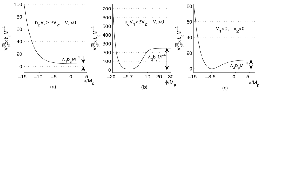
Figure 1: Three possible shapes of the effective potential $V_{eff}^{(0)}(\phi)$ in the models with $b_{g}V_{1}>V_{2}$:  Fig.(a)   $b_{g}V_{1}\geq 2V_{2}$ (in the graph $V_{1}=10M^{4}$ and $V_{2}=4b_{g}M^{4}$);  Fig.(b)   $b_{g}V_{1}<2V_{2}$ (in the graph $V_{1}=10M^{4}$ and $V_{2}=9.9b_{g}M^{4}$). The value of $V_{eff}^{(0)}$ in the minimum $\phi_{min}=-5.7M_{p}$ is larger than zero;  Fig.(c)   $V_{1}<0$, $V_{2}<0$ (in the graph $V_{1}=-30M^{4}$ and $V_{2}=-50b_{g}M^{4}$). $V_{eff}^{(0)}(\phi_{min})=0$ in the minimum $\phi_{min}=-8.5M_{p}$ . In all the cases here as well as in all solutions presented in this paper we choose $\alpha=0.2$.

So let us study spatially flat FRW cosmological models governed by the system of equations

$$\frac{\dot{a}^{2}}{a^{2}}=\frac{1}{3M_{p}^{2}}\rho$$ (30)

and (20)-(22) where one should set $\delta=0$.

In the fine tuned case under consideration, the constraint (16) yields

$$\zeta=\zeta(\phi,X;M)|_{\delta=0}\equiv b_{g}-\frac{2V_{2}}{V_{1}+M^{4}e^{-2\alpha\phi/M_{p}}},$$ (31)

The energy density and pressure take then the canonical form,

$$\rho|_{\delta=0}=\frac{1}{2}\dot{\phi}^{2}+V_{eff}^{(0)}(\phi);\qquad p|_{\delta=0}=\frac{1}{2}\dot{\phi}^{2}-V_{eff}^{(0)}(\phi),$$ (32)

where the effective potential of the scalar field $\phi$ results from Eq.(14)

$$V_{eff}^{(0)}(\phi)\equiv V_{eff}(\phi;\zeta,M)|_{\delta=0}=\frac{[V_{1}+M^{4}e^{-2\alpha\phi/M_{p}}]^{2}}{4[b_{g}\left(V_{1}+M^{4}e^{-2\alpha\phi/M_{p}}\right)-V_{2}]}$$ (33)

and the $\phi$-equation (22) is reduced to

$$\ddot{\phi}+3H\dot{\phi}+\frac{dV^{(0)}_{eff}}{d\phi}=0.$$ (34)

Notice that $V_{eff}^{(0)}(\phi)$ is non-negative for any $\phi$ provided

$$b_{g}V_{1}\geq V_{2},$$ (35)

that we will assume in this paper.

In the following three subsections we consider three different dilaton-gravity cosmological models determined by different choice of the parameters $V_{1}$ and $V_{2}$: one model with $V_{1}<0$ and two models with $V_{1}>0$. The appropriate three possible shapes of the effective potential $V_{eff}^{(0)}(\phi)$ are presented in Fig.1. A special case with the fine tuned condition $b_{g}V_{1}=V_{2}$ is discussed in Appendix B where we show that equality of the couplings to measures $\Phi$ and $\sqrt{-g}$ in the action (equality $b_{g}V_{1}=V_{2}$ is one of the conditions for this to happen) gives rise to a symmetric form of the effective potential.

IV.2 Model with $V_{1}<0$ and $V_{2}<0$

IV.2.1 Resolution of the Old Cosmological Constant Problem in TMT

The most remarkable feature of the effective potential (33) is that it is proportional to the square of $V_{1}+M^{4}e^{-2\alpha\phi/M_{p}}$ which is a straightforward consequence of our basic assumption that $L_{1}$ and $L_{2}$ are independent of the measure fields (see item 2 in Sec.II, Eq.(14) and the discussion after it). Due to this, as $V_{1}<0$ and $V_{2}<0$, the effective potential has a minimum where it equals zero automatically, without any further tuning of the parameters $V_{1}$ and $V_{2}$ (see also Fig.1c). This occurs in the process of evolution of the field $\phi$ at the value of $\phi=\phi_{0}$ where

$$V_{1}+M^{4}e^{-2\alpha\phi_{0}/M_{p}}=0.$$ (36)

This means that the universe evolves into the state with zero cosmological constant without any additional tuning of the parameters and initial conditions.

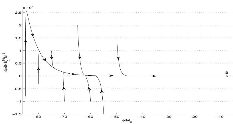
Figure 2: Phase portrait (plot of $\frac{d\phi}{dt}$ versus $\phi$) for the model with $V_{1}<0$ and $V_{2}<0$. All phase curves started with $|\phi|\gg M_{p}$ quickly approach the attractor long before entering the oscillatory regime. The region of the oscillatory regime is marked by point $B$. The oscillation spiral is not visible here because of the chosen scales along the axes.

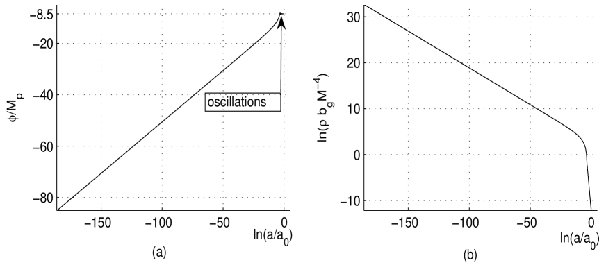
Figure 3: (a) Typical dependence of the field $\phi$ (fig. (a)) and the energy density $\rho$ (fig. (b)) upon $\ln(a/a_{0})$. Here and in all the graphs of this paper describing scale factor $a$ dependences, $a(t)$ is normalized such that at the end point of the described process $a(t_{end})=a_{0}$. In the model with $V_{1}<0$ the power law inflation ends with damped oscillations of $\phi$ around $\phi_{0}$ determined by Eq.(36). For the choice $V_{1}=-30M^{4}$ Eq.(36) gives $\phi_{0}=-8.5M_{p}$ . (b) The exit from the early inflation is accompanied with approaching zero of the energy density $\rho$. The graphs correspond to the evolution which starts from the initial values $\phi_{in}=-85M_{p}$, $\dot{\phi}_{in}=-8\cdot 10^{5}M^{2}/\sqrt{b_{g}}$.

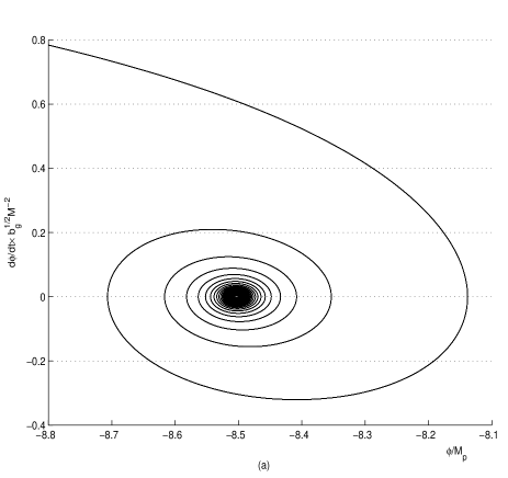
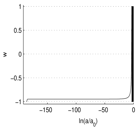
Figure 4: Fig.(a) zoom in on the oscillatory regime which marked by point B in Fig.2.   (b) Equation-of-state $w=p/\rho$ as function of the scale factor for the parameters and initial conditions as in Fig.3. Most of the time the expansion of the universe is a power law inflation with almost constant $w\approx-0.95$; $w$ oscillates between $-1$ and $1$ at the exit from inflation stage, i.e. as $\phi\rightarrow\phi_{0}$ and $\rho\rightarrow 0$.

To provide the global scale invariance (8), the prepotentials $V_{1}$ and $V_{2}$ enter in the action (9) with factor $e^{2\alpha\phi/M_{p}}$. However, if quantum effects (considered in the original frame) break the scale invariance of the action (9) via modification of existing prepotentials or by means of generation of other prepotentials with arbitrary $\phi$ dependence (and in particular a ”normal” cosmological constant term $\int\tilde{\Lambda}\sqrt{-g}d^{4}x$), this cannot change the result of TMT that the effective potential generated in the Einstein frame is proportional to a perfect square. Note that the assumption of scale invariance is not necessary for the effect of appearance of the perfect square in the effective potential in the Einstein frame and therefore for the described mechanism of disappearance of the cosmological constant, see Refs.GK2 -G1 .

If such type of the structure for the scalar field potential in a conventional (non TMT) model would be chosen ”by hand” it would be a sort of fine tuning. But in our TMT model it is not the starting point, it is rather a result obtained in the Einstein frame of TMT models with spontaneously broken shift symmetry (11).

At the first glance this effect contradicts the Weinberg’s no-go theoremWeinberg1 which states that there cannot exist a field theory model where the cosmological constant is zero without fine tuning. In Sec.VIIIB we will study in detail the manner our TMT model avoids this theorem.

IV.2.2 Cosmological Dynamics

As $M^{4}e^{-2\alpha\phi/M_{p}}\gg Max\left(|V_{1}|,|V_{2}|/b_{g}\right)$, the effective potential (33) behaves as the exponential potential $V_{eff}^{(0)}\approx\frac{1}{4b_{g}}M^{4}e^{-2\alpha\phi/M_{p}}$. So, as $\phi\ll-M_{p}$ the model describes the well studied power law inflation of the early universepower-law -Halliwell if $0<\alpha<1/\sqrt{2}$ :

$$a(t)=a_{in}\left(\frac{t}{t_{in}}\right)^{1/2\alpha^{2}},\qquad\phi(t)=\frac{M_{p}}{\alpha}ln\left(\frac{\alpha^{2}M^{2}t}{M_{p}\sqrt{b_{g}(3-2\alpha^{2})}}\right).$$ (37)

The only true integration constant in this exact analytic solutionLiddle is the initial value of the scale factor $a_{in}=a(t_{in})$ where $t_{in}>0$. The choice of $t_{in}$ determines both the initial value of $\phi_{in}=\phi(t_{in})$ and the initial value of $\dot{\phi}_{in}=\dot{\phi}(t_{in})$. Therefore the initial values $\phi_{in}$ and $\dot{\phi}_{in}$ cannot be chosen independently. This feature of the solutions (37) corresponds to the fact that in the phase plane $(\phi,\dot{\phi})$ there is only one phase curve representing these solutions and it plays the role of the attractorHalliwell for all other solutions with arbitrary initial values of $\phi_{in}$ and $\dot{\phi}_{in}$. Excluding time from $\phi(t)$ and $\dot{\phi}(t)$ we obtain the equation of the attractor in the phase plane:

$$\frac{\sqrt{b_{g}}}{M^{2}}\,\dot{\phi}=\frac{\alpha}{\sqrt{3-2\alpha^{2}}}e^{-\alpha\phi/M_{p}}.$$ (38)

In all points of the attractor (38) the ratio

$$n\equiv\frac{V_{eff}^{(0)}}{\dot{\phi}^{2}/2}=\frac{3}{2\alpha^{2}}-1$$ (39)

is constant and $n>2$ in the case of the power law inflation, i.e. if $\alpha<1/\sqrt{2}$. With our choice of $\alpha=0.2$, we have along the attractor (38) $n=36.5$ and the equation-of-state $w\approx-0.95$.

Note also that for the exact power law inflating solutions (37), $\dot{\phi}$ is always positive. Phase curves corresponding to different independent initial values $\phi_{in}$ and $\dot{\phi}_{in}$ (including negative $\dot{\phi}_{in}$) and obtained by means of numerical solutions are presented in Fig.2. One can see that their shapes are characterized by much steeper (almost vertical) approaching the attractor than the exponential shape of the decay of the attractor itself. Note that in Fig.2 we have presented only phase curves started from points $(\phi_{in},\dot{\phi}_{in})$ where $\frac{1}{2}\dot{\phi}_{in}^{2}\sim V_{eff}^{(0)}(\phi_{in})$. We have checked that the same very steep approach to the attractor is peculiar also to the phase curves started from points $(\phi_{in},\dot{\phi}_{in})$ where $\frac{1}{2}\dot{\phi}_{in}^{2}\gg V_{eff}^{(0)}(\phi_{in})$.

Further behavior of the solutions is qualitatively evident enough. With the choice $\alpha=0.2$, $V_{1}=-30M^{4}$ and $V_{2}=-50b_{g}M^{4}$, the results of numerical solutions are presented in Figs. 2, 3 and 4. Exit from the inflation regime starts as $\phi$ becomes close to $\phi_{0}$ determined by Eq.(36). Then the energy density starts to tend to zero very fast, Fig.3b. The numerical solutions show that for all phase curves corresponding to initial conditions with $\phi_{in}\ll-M_{p}$ and arbitrary $\dot{\phi}_{in}$, the exit from the inflation occurs when these phase curves practically coincide with the attractor. The process ends with oscillatory regime, Fig.4a, where $\phi$ performs damped oscillations around the minimum of the effective potential (see also Fig.1c).

IV.3 Model with $V_{1}>0$ and $b_{g}V_{1}>2V_{2}$: Early Power Law Inflation Ending With Small $\Lambda$ Driven Expansion

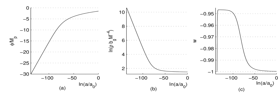
Figure 5: The values of $V_{1}$ and $V_{2}$ are as in Fig.1a. The graphs correspond to the initial conditions $\phi_{in}=-30M_{p}$, $\dot{\phi}_{in}=-5M^{2}b_{g}^{-1/2}$. The early universe evolution is governed by the almost exponential potential (see Fig.1a) providing the power low inflation ($w\approx-0.95$ interval in fig.(c)). After transition to the late time universe the scalar $\phi$ increases with the rate typical for a quintessence scenario. Later on the cosmological constant $\Lambda_{1}$ becomes a dominant component of the dark energy that is displayed by the infinite region where $w\approx-1$ in fig.(c).

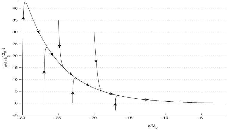
Figure 6: Phase portrait (plot of $\frac{d\phi}{dt}$ versus $\phi$) for the model with $b_{g}V_{1}>2V_{2}$. All trajectories approach the attractor which in its turn asymptotically (as $\phi\rightarrow\infty$) takes the form of the straight line $\dot{\phi}=0$.

In this model the effective potential (33) is a monotonically decreasing function of $\phi$ (see Fig.1a). As $\phi\ll-M_{p}$ the model describes the power law inflation (37), similar to what we discussed in the model of previous subsection.

Applying this model to the cosmology of the late time universe and assuming that the scalar field $\phi\rightarrow\infty$ as $t\rightarrow\infty$, it is convenient to represent the effective potential (33) in the form

$$V_{eff}^{(0)}(\phi)=\Lambda_{1}+V_{q-l}(\phi)\qquad\text{where}\qquad\Lambda_{1}=\Lambda|_{b_{g}V_{1}>2V_{2}},$$ (40)

with the definition

$$\Lambda=\frac{V_{1}^{2}}{4(b_{g}V_{1}-V_{2})}.$$ (41)

Here $\Lambda$ is the positive cosmological constant (see (35)) and

$$V^{(0)}_{q-l}(\phi)=\frac{(b_{g}V_{1}-2V_{2})V_{1}M^{4}e^{-2\alpha\phi/M_{p}}+(b_{g}V_{1}-V_{2})M^{8}e^{-4\alpha\phi/M_{p}}}{4(b_{g}V_{1}-V_{2})[b_{g}(V_{1}+M^{4}e^{-2\alpha\phi/M_{p}})-V_{2}]},$$ (42)

that is the evolution of the late time universe is governed both by the cosmological constant $\Lambda_{1}$ and by the quintessence-like potential $V^{(0)}_{q-l}(\phi)$.

Thus the effective potential (33) provides a possibility for a cosmological scenario which starts with a power law inflation and ends with a cosmological constant $\Lambda_{1}$. The smallness of $\Lambda_{1}$ may be achieved without fine tuning of dimensionfull parameters, that will be discussed in Sec.VIA. Such scenario may be treated as a generalized quintessential inflation type of scenario. Recall that the $\phi$-dependence of the effective potential (33) appears here only as the result of the spontaneous breakdown of the global scale symmetry.

Results of numerical solutions for such type of scenario are presented in Figs.5 and 6 ($V_{1}=10M^{4}$, $V_{2}=4b_{g}M^{4}$) The early universe evolution is governed by the almost exponential potential (see Fig.1a) providing the power low inflation ($w\approx-0.95$ interval in Fig.5c). The choice of $V_{1}$ and $V_{2}$ such that $b_{g}V_{1}\geq 2V_{2}$ provides a graceful exit from inflation with transition to the late time universe where the scalar $\phi$ increases with the rate typical for a quintessence scenario. Later on the cosmological constant $\Lambda_{1}$ becomes a dominant component of the dark energy that is displayed by the infinite region where $w\approx-1$ in Fig.5c. The phase portrait in Fig.3 shows that all the trajectories started with $|\phi|\gg M_{p}$ quickly approach the attractor which asymptotically (as $\phi\rightarrow\infty$) takes the form of the straight line $\dot{\phi}=0$. Qualitatively similar results are obtained also when $V_{1}$ is positive but $V_{2}$ is negative.

IV.4 Model with $V_{1}>0$ and $V_{2}<b_{g}V_{1}<2V_{2}$

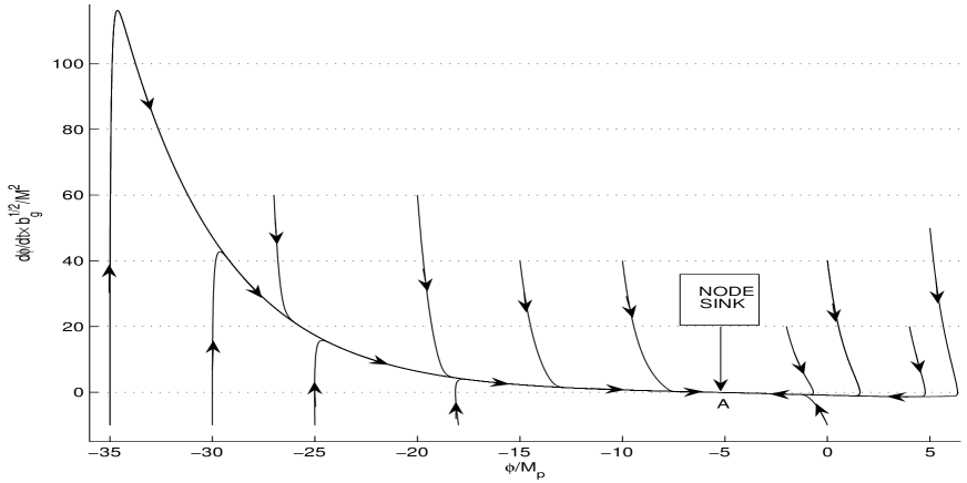
Figure 7: Phase portrait (plot of $\frac{d\phi}{dt}$ versus $\phi$) for the model with $V_{2}<b_{g}V_{1}<2V_{2}$ and $V_{1}>0$ (the parameters are chosen here as in Fig.1b ). Trajectories started anywhere in the phase plane in a finite time end up at the same point $A(-5.7,0)$ which is a node sink. There exist two attractors ending up at $A$, one from the left and other from the right. All phase curves starting with $|\phi|\gg M_{p}$ quickly approach these attractors.

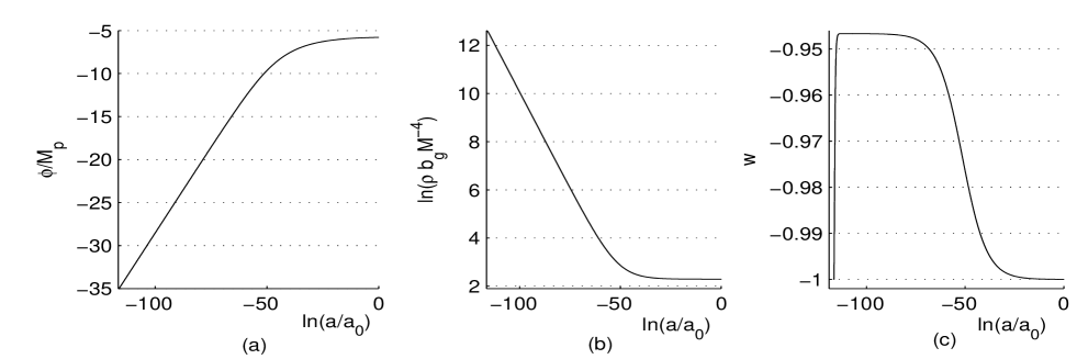
Figure 8: Cosmological dynamics in the model with $V_{2}<b_{g}V_{1}<2V_{2}$ and $V_{1}>0$: typical dependence of $\phi$ (Fig.(a)), the energy density $\rho$ (Fig.(b)) and the equation-of-state $w$ (Fig.(c)) upon $\ln(a/a_{0})$ where the scale factor $a(t)$ normalized as in Fig.3. The graphs correspond to the initial conditions $\phi_{in}=-35M_{p}$, $\dot{\phi}_{in}=-10b_{g}^{-1/2}M^{2}$. The early universe evolution is governed by an almost exponential potential (see Fig.1b) providing the power low inflation ($w\approx-0.95$ interval in Fig.(c)). After arriving the minimum of the potential at $\phi_{min}=-5.7M_{p}$ (see Fig.1b and the point $A(-5.7M_{p},0)$ of the phase plane in Fig.4) the scalar $\phi$ remains constant. At this stage the dynamics of the universe is governed by the constant energy density $\rho=V^{(0)}_{eff}(\phi_{min})$ (see the appropriate intervals $\rho=const$ in Fig.(b) and $w=-1$ in Fig.(c)).

In this case the effective potential (33) has the minimum (see Fig.1b)

$$V^{(0)}_{eff}(\phi_{min})=\frac{V_{2}}{b_{g}^{2}}\qquad\text{at}\qquad\phi=\phi_{min}=-\frac{M_{p}}{2\alpha}\ln\left(\frac{2V_{2}-b_{g}V_{1}}{b_{g}}\right).$$ (43)

For the choice of the parameters as in Fig.1b, i.e. $V_{1}=10M^{4}$ and $V_{2}=9.9b_{g}M^{4}$, the minimum is located at $\phi_{min}=-5.7M_{p}$. The character of the phase portrait one can see in Fig.7.

For the early universe as $\phi\ll-M_{p}$, similar to what we have seen in the models of the previous two subsections, the model implies the power law inflation. However, the phase portrait Fig.7 shows that now all solutions end up without oscillations at the minimum $\phi_{min}=-5.7M_{p}$ with $\frac{d\phi}{dt}=0$. In this final state of the scalar field $\phi$, the evolution of the universe is governed by the cosmological constant $V^{(0)}_{eff}(\phi_{min})$ determined by Eq.(43). For some details of the cosmological dynamics see Fig.8. The desirable smallness of $V^{(0)}_{eff}(\phi_{min})$ can be provided again without fine tuning of the dimensionfull parameters that will be discussed in Sec.VIA. The absence of appreciable oscillations in the minimum is explained by the following two reasons: a) the non-zero friction at the minimum determined by the cosmological constant $V^{(0)}_{eff}(\phi_{min})$; b) the shape of the potential near to minimum is too flat.

The described properties of the model are evident enough. Nevertheless we have presented them here because this model is a particular (fine tuned) case of an appropriate model with $\delta\neq 0$ studied in Sec.VII where we will demonstrate a possibility of states with $w<-1$ without any exotic contributions, like a phantom term, in the original action.

V TMT Cosmology With No Fine Tuning I:
Absence of the Initial Singularity of the Curvature and Inflationary Cosmology with Graceful Exit to $\Lambda=0$ Vacuum

V.1 General Analysis and Numerical Solutions

In the following three sections we return to the general case of our model (see Sec.III) with no fine tuning of the parameters $b_{g}$ and $b_{\phi}$, i.e. the parameter $\delta$, defined by Eq.(17), is non zero. Then the dynamics of the FRW cosmology is described by Eqs.(20)-(22) and (30). Let us start from the analysis of Eq.(22). The interesting feature of this equation is that each of the factors $Q_{i}(\phi,X)$   ($i=1,2,3$) can get to zero and this effect depends on the range of the parameter space chosen. This is the origin of drastic changes of the topology of the phase plane comparing with the fine tuned models of Sec.IV.

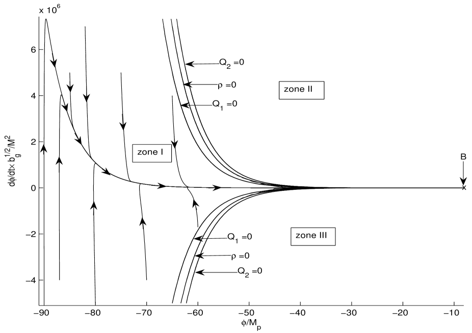
Figure 9: The phase portrait for the model with $\delta=0.1$, $\alpha=0.2$, $V_{1}=-30M^{4}$ and $V_{2}=-50b_{g}M^{4}$. All phase curves demonstrate the attractor behavior similar to that in the fine tuned case $\delta=0$, Fig.2. One can see that the attractor does not intersect the line $Q_{1}=0$, see also Fig.10. The location of the oscillatory regime marked by point $B$ is exactly the same as in the model with $\delta=0$. The essential difference consists in a novel topological structure: in the neighborhood of the line $Q_{1}=0$ all the phase curves exhibit a repulsive behavior from this line and therefore points of the line $Q_{1}=0$ are dynamically unachievable. Hence the phase curves cannot be continued infinitely to the past.

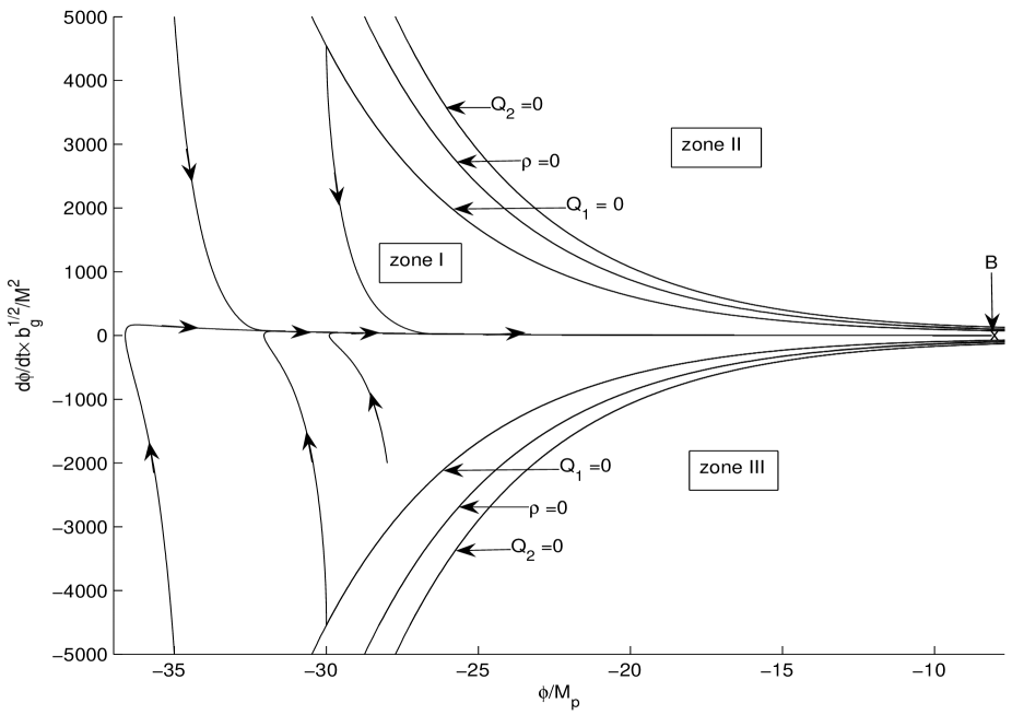
Figure 10: The same phase portrait as in Fig.9 but with more clear exhibition of the structure of the phase plane near to the point $B$.

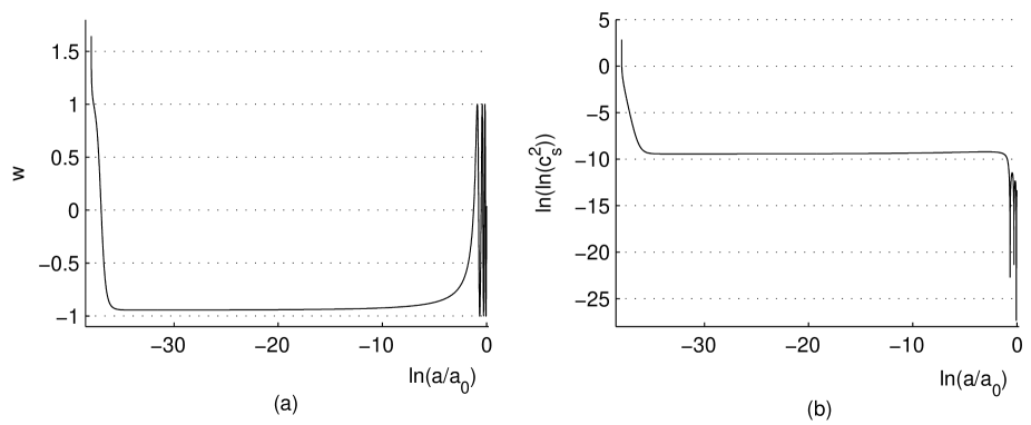
Figure 11: Typical scale factor dependence of the equation-of-state $w$ and the squared sound speed $c^{2}_{s}$ for the phase curves starting from points very close to the line $Q_{1}=0$ (in this figure - for $\phi_{in}=-30M_{p}$ and $\dot{\phi}_{in}=4540.7569b_{g}^{-1/2}M^{2}$). The squared sound speed in the starting point is $c^{2}_{s}\approx exp(exp(2.86))\approx 3.8\cdot 10^{7}$. It is not a problem to obtain more than 75 e-folds during the power law inflation (the region of $w\approx-0.95$ in Fig.(a)) just by choosing a larger absolute value $|\phi_{in}|$. We have chosen $\phi_{in}=-30M_{p}$ because this allows to show more details in these and subsequent graphs.

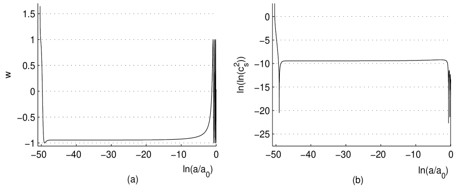
Figure 12: The same as in Fig.11 but for $\phi_{in}=-30M_{p}$ and $\dot{\phi}_{in}=-4540.7569b_{g}^{-1/2}M^{2}$. The squared sound speed in the starting point is also $c^{2}_{s}\approx exp(exp(2.86))\approx 3.8\cdot 10^{7}$.

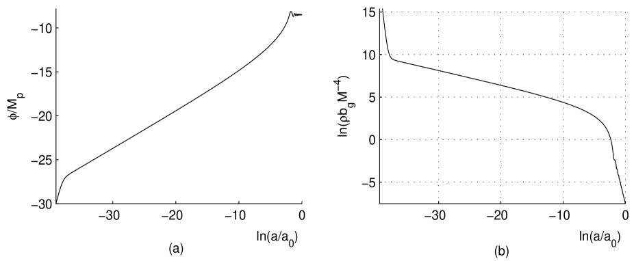
Figure 13: Typical scale factor dependence of $\phi$ and $\rho$ for the phase curves starting from points very close to the line $Q_{1}=0$ (in this figure - for $\phi_{in}=-30M_{p}$ and $\dot{\phi}_{in}=4540.7569b_{g}^{-1/2}M^{2}$).

For $Q_{1}\neq 0$, Eqs. (22), (30) result in the well known equationVikman

$$\ddot{\phi}+\frac{\sqrt{3\rho}}{M_{p}}c_{s}^{2}\dot{\phi}+\frac{\rho_{,\phi}}{\rho_{,X}}=0,$$ (44)

where $c_{s}$ is the effective sound speed of perturbationsGM

$$c_{s}^{2}=\frac{p_{,X}}{\rho_{,X}}=\frac{Q_{2}}{Q_{1}},$$ (45)

$$\frac{\rho_{,\phi}}{\rho_{,X}}=-\frac{\alpha}{M_{p}}\cdot\frac{Q_{3}}{Q_{1}}\cdot M^{4}e^{-2\alpha\phi/M_{p}};$$ (46)

$\rho$ and $p$ are defined by Eqs.(20), (21) and $Q_{i}$ $(i=1,2,3)$ - by Eqs.(24)-(26).

It follows from the definitions of $Q_{1}$ and $Q_{2}$ that $c_{s}^{2}>1$ when $Q_{1}>0$ and $X>0$ (that implies $Q_{2}>0$). Therefore in the cosmological FRW background, the sound speed of perturbations can be bigger than speed of light, . However $c_{s}^{2}<1$ when $Q_{1}<0$ and $Q_{2}<0$.

In the model with $V_{1}<0$ and $V_{2}<0$ (the fine tuned version of which has been studied in Sec.IVB), the structure of the phase plane is presented in Figs.9 and 10 for the following set of the parameters: $\alpha=0.2$, $\delta=0.1$, $V_{1}=-30$, $V_{2}=-50$. With such a choice of the parameters the following condition is satisfied

$$(b_{g}+b_{\phi})V_{1}-2V_{2}>0$$ (47)

that determines the structure of the phase plane. By the two branches of the line $Q_{1}=0$, the phase plane is divided into three large dynamically disconnected zones. In the most part of two of them (II and III), the energy density is negative ($\rho<0$). In the couple of regions between the lines $Q_{1}=0$ and $\rho=0$ that we refer for short as ($Q_{1}\rightarrow\rho$)-regions, $\rho>0$ but $Q_{1}<0$. Typical scale factor dependence of the equation-of-state $w$, the sound speed of perturbations $c_{s}^{2}$, the inflaton $\phi$ and the energy density $\rho$ are presented in Figs.11, 12 and 13. It is not a problem to obtain more than 75 e-folds during the power law inflation (the region of $w\approx-0.95$ in Fig.11a) just by choosing a larger absolute value $|\phi_{in}|$. We have chosen $\phi_{in}=-30M_{p}$ because this allows to show more details in these graphs.

The zone I of the phase plane (where $Q_{1}>0$, $\rho>0$ and $Q_{2}>0$) is of a great cosmological interest:

• Similar to what we have seen in the fine tuned model of Sec.IVB, all the phase curves start with very steep approach to an attractor. The nonlinearity in $X$ does not allow to obtain an exact analytic solution in the model under consideration and therefore we have no here the analytic equation of the attractor. But taking into account Eq.(39), it becomes evident that, with our choice of the parameters $\alpha$ and $\delta$, the emergence of the additional terms $\propto\delta X$ and $\propto\delta^{2}X^{2}$ in the model under consideration results in small enough corrections to the equation of the attractor in comparison with Eq.(38) of the fined tuned model of Sec.IVB. For our qualitative analysis below one can use Eq.(38) as a good approximation to the true attractor equation.

• Comparing the equation of the line $Q_{1}=0$, which for $\phi\ll-M_{p}$ can be written in the form

  $$\frac{\sqrt{b_{g}}}{M^{2}}\,\dot{\phi}=\pm\frac{1}{\delta}\sqrt{\frac{2}{3}(2-\delta)}\cdot e^{-\alpha\phi/M_{p}}+{\cal O}\left(\frac{V_{1}}{M^{4}}e^{\alpha\phi/M_{p}}\right),$$ (48)

  with the equation of the attractor which approximately coincides with Eq.(38), we see that the upper brunch of the line $Q_{1}=0$ has actually the same form of a decaying exponent as the attractor, but the factor in front of the exponent in Eq.(48) is about $10^{2}$ times bigger than in Eq.(38). The above analytic estimations are confirmed by the numerical solutions as one can see in Fig.9. This means that the attractor does not intersect the line $Q_{1}=0$. Therefore all the phase curves starting in zone I arrive at the attractor (of course asymptotically).

• In the neighborhood of the line $Q_{1}=0$ all the phase curves exhibit a repulsive behavior from this line. In other words, the shape of two branches of $Q_{1}=0$ do not allow a classical dynamical continuation of the phase curves backward in time without crossing the classical barrier formed by the line $Q_{1}=0$. This is true for all finite values of the initial conditions $\phi_{in}$, $\dot{\phi}_{in}$ in zone I.

• Similar to what we have seen already in the model with $\delta=0$ of Sec.IVB, the power law inflation ends with the graceful exit to a zero CC vacuum state without fine tuning.

• As one can see from Figs.11 and 12, the initial stage of evolution is very much different from the subsequent one, that is a power law inflation. This fact may have a relation to the results of the study of completeness of inflationary cosmological models in past directionsBGV .

• If the phase curves start from points $(\phi_{in},\dot{\phi}_{in})$ in zone I very close to the line $Q_{1}=0$ then the sound speed of perturbations has huge values at the beginning of the evolution, see Figs.11b and 12b. However in the power law inflation stage, $c_{s}$ is too close to the speed of light and appears to be unable to increase the tensor-to-scalar perturbation ratioGM , Mukh-Vik-JCAP .

In two regions between the lines $Q_{1}=0$ and $Q_{2}=0$ that we refer for short as ($Q_{1}\rightarrow Q_{2}$)-regions,, the squared sound speed of perturbations is negative, $c_{s}^{2}<0$. This means that on the right hand side of the classical barrier $Q_{1}=0$, the model is absolutely unstable. Moreover, this pure imaginary sound speed becomes infinite in the limit $Q_{1}\rightarrow 0-$. Thus the branches of the line $Q_{1}=0$ divide zone I (of the classical dynamics) from the ($Q_{1}\rightarrow Q_{2}$)-regions where the physical significance of the model is unclear. Note that the line $\rho=0$ divides the ($Q_{1}\rightarrow Q_{2}$)-regions into two subregions with opposite signs of the classical energy density.

Thus the structure of the phase plane yields a conclusion that the starting point of the classical history in the phase plane can be only in zone I and the line $Q_{1}=0$ is the limiting set of points where the classical history might begin. For any finite initial values of $\phi_{in}$ and $\dot{\phi}_{in}$ at the initial cosmic time $t_{in}$, the duration $t_{in}-t_{s}$ of the continuation of the evolution into the past up to the moment $t_{s}$ when the phase trajectory arrives the line $Q_{1}=0$, is finite.

V.2 Analysis of the Initial Singularity

Let us analyze what happens as $t\to t_{s}$ (and $Q_{1}(\phi,\dot{\phi})\to 0$) if this continuation to the past starts from a point in zone I of the phase plane with finite initial values $\phi_{in}$ and $\dot{\phi}_{in}$ . First note that the energy density $\rho_{s}=\rho(t_{s})$ and the pressure $p_{s}=p(t_{s})$ are finite in all the points of the line $Q_{1}=0$ with finite coordinates $\phi_{s}=\phi(t_{s})$, $\dot{\phi_{s}}=\dot{\phi}(t_{s})$, that it is easy to see from Eqs.(20), (21) and (24). The strong energy condition is satisfied in regions of zone I close to the line $Q_{1}=0$ including the line itself. In fact, for any unit time-like vector $t^{\mu}$ we have on the line $Q_{1}=0$

$$\left(T_{\mu\nu}^{eff}-\frac{1}{2}\tilde{g}_{\mu\nu}T^{eff}\right)t^{\mu}t^{\nu}=\frac{1}{2}(\rho_{s}+3p_{s})\approx\frac{2b_{\phi}}{(b_{g}-b_{\phi})^{2}}M^{4}e^{-2\alpha\phi_{s}/M_{p}}>0,$$ (49)

where $T_{\mu\nu}^{eff}$ is defined in Eq.(19), $T^{eff}\equiv\tilde{g}^{\mu\nu}T_{\mu\nu}^{eff}$ and we have taken into account our choice of the parameters ($b_{g}>0$, $b_{\phi}>0$ and Eq.(35)) and assumed that $M^{4}e^{-2\alpha\phi_{s}/M_{p}}\gg|V_{1}|$. This result is in the total agreement with the numerical solutions of the previous subsection. In particular, the described analytic approximation on the line $Q_{1}=0$ yields $w_{s}=p_{s}/\rho_{s}\approx 5/3$ which is in a very good agreement with the numerical results obtained in regions of zone I close enough to the line $Q_{1}=0$, see Figs.11a and 12a.

It follows from the Einstein equations (30) and

$$\frac{\ddot{a}}{a}=-\frac{1}{6M_{p}^{2}}(\rho+3p)$$ (50)

that the first and second time derivatives of the scale factor, $\dot{a}_{s}=\dot{a}(t_{s})$ and $\ddot{a}_{s}=\ddot{a}(t_{s})$, and therefore the curvature, are finite on the line $Q_{1}=0$. The time derivative of the energy density also approaches a finite value

$$\dot{\rho}_{s}=3\frac{\dot{a}_{s}}{a_{s}}(\rho_{s}+p_{s})<\infty$$ (51)

It is interesting to see how this result follows from the scalar field dynamics. Using Eqs.(20), (24) and (27) we obtain

$$\dot{\rho}=\rho,_{\phi}\cdot\dot{\phi}+\rho,_{X}\cdot\dot{X}=-\frac{\alpha}{2M_{p}}\cdot\frac{M^{4}e^{-2\alpha\phi/M_{p}}}{b_{g}(M^{4}e^{-2\alpha\phi/M_{p}}+V_{1})-V_{2}}\cdot Q_{3}+\frac{Q_{1}}{2[b_{g}(M^{4}e^{-2\alpha\phi/M_{p}}+V_{1})-V_{2}]}\cdot\dot{\phi}\ddot{\phi}$$ (52)

The first term in the r.h.s. of Eq.(52) is evidently finite on the line $Q_{1}=0$. To analyze the behavior of the second term in the r.h.s. of Eq.(52) one should note that the last two terms of Eq.(22) remain finite as $t\to t_{s}$ and $Q_{1}(\phi(t),\dot{\phi}(t))\to 0$. We infer from this that

$$|\ddot{\phi}|\to\infty$$ (53)

but in such a way that

$$Q_{1}\ddot{\phi}\to\text{finite value depending on}\,\phi_{s}\,\text{and}\,\dot{\phi}_{s}.$$ (54)

Therefore the second term in the r.h.s. of Eq.(52) has a finite limit too.

Similar manipulations for $\dot{p}$ give

$$\dot{p}=p,_{\phi}\cdot\dot{\phi}+p,_{X}\cdot\dot{X}$$ (55)

where again the first term is evidently finite on the line $Q_{1}=0$ but for the second term we have using Eq.(25 )

$$p,_{X}\cdot\dot{X}=\frac{Q_{2}}{2[b_{g}(M^{4}e^{-2\alpha\phi/M_{p}}+V_{1})-V_{2}]}\cdot\dot{\phi}\ddot{\phi}$$ (56)

Recall that $Q_{2}>0$ in zone I including the line $Q_{1}=0$. Moreover, the analysis of the phase curves in Figs.9 and 10 shows that if $\dot{\phi}_{in}>0$ than $\ddot{\phi}_{in}<0$ and vice versa. Thus we conclude that

$$\dot{p}\to-\infty\qquad as\qquad t\to t_{s}$$ (57)

It is now clear from Eq.(50) that the third time derivative of the scale factor is singular at $t=t_{s}$:

$$\frac{\dddot{a}}{a}\approx-\frac{\dot{p}}{2M_{p}^{2}}\to\infty\qquad as\qquad t\to t_{s}$$ (58)

Therefore although the scalar curvature

$$R=-6(\frac{\ddot{a}}{a}+\frac{\dot{a}^{2}}{a^{2}})$$ (59)

is finite as $t\to t_{s}$ but its time derivative is singular:

$$\dot{R}\approx-6\frac{\dddot{a}}{a}\to-\infty\qquad\text{as}\qquad t\to t_{s}$$ (60)

The regular behavior of $\dot{a}$ and $\ddot{a}$ together with singularity of $\dddot{a}$ implies that

$$a(t)\approx a_{s}+A(t-t_{s})^{n}\qquad\text{as}\qquad t\to t_{s},\qquad where\qquad 2<n<3$$ (61)

and $A>0$ is a constant. This type of singularity we discover here in the framework of the dynamical model is present in the classification of ”sudden” singularities given by BarrowBarrow1 on purely kinematic grounds.

We are going now to solve the equations of motion in order to find out the value of $n$ in Eq.(61). For this, as $t$ is very close to $t_{s}$ one can represent $\phi(t)$ and $\dot{\phi}(t)$ in the form $\phi(t)=\phi_{s}+\frac{M_{p}}{2\alpha}\chi$, $\dot{\phi}(t)=\dot{\phi}_{s}+\frac{M_{p}}{2\alpha}\dot{\chi}$ where $|\chi|\ll\frac{2\alpha}{M_{p}}|\phi_{s}|$ and $|\dot{\chi}|\ll\frac{2\alpha}{M_{p}}|\dot{\phi}_{s}|$. Then keeping in the $\phi$-equation (22) only leading terms as $t\to t_{s}$, we obtain

$$\dot{\chi}\cdot\ddot{\chi}\approx B,$$ (62)

where the constant $B$ is defined by

$$B=\frac{4\alpha^{2}}{\delta^{2}b_{g}^{2}M_{p}^{2}}\left[H_{s}Q_{2}^{(s)}-\frac{\alpha Q_{3}^{(s)}}{3M_{p}\dot{\phi}_{s}}M^{4}e^{-2\alpha\phi_{s}/M_{p}}\right],$$ (63)

$H_{s}$ is the Hubble parameter at $t=t_{s}$ and $Q_{i}^{(s)}=Q(\phi_{s},\dot{\phi}_{s})>0$,   $i=2,3$. Eq.(62) results in

$$\dot{\phi}=\dot{\phi}_{s}\pm\frac{M_{p}}{2\alpha}\sqrt{2B(t-t_{s})}$$ (64)

provided $B>0$. If we study the evolution starting from $\dot{\phi}_{in}<0$ then the nearest $\dot{\phi}_{s}<0$ and $B>0$ without any additional restrictions on the parameters. However if the evolution starts from $\dot{\phi}_{in}>0$ then the nearest $\dot{\phi}_{s}>0$ and one should test whether the condition $B>0$ implies additional restrictions on the parameters. Using Eqs.(20), (30), (25) and (26) one can show that for $\dot{\phi}_{s}>0$

$$B=\frac{8\alpha^{2}}{9\sqrt{6}\delta^{3}b_{g}^{4}\sqrt{b_{g}+b_{\phi}}}\cdot[\sqrt{6}(b_{g}+b_{\phi})(b_{g}^{2}+b_{\phi}^{2})-2\alpha b_{g}(b_{g}^{2}+b_{\phi}^{2}-b_{g}b_{\phi})]\frac{M^{6}}{M_{p}^{3}}e^{-3\alpha\phi_{s}/M_{p}}$$ (65)

Therefore $B>0$ if

$$\alpha<\sqrt{\frac{3}{2}}\cdot\frac{(b_{g}+b_{\phi})(b_{g}^{2}+b_{\phi}^{2})}{b_{g}(b_{g}^{2}+b_{\phi}^{2}-b_{g}b_{\phi})}$$ (66)

The inequality (66) provides that the condition $\alpha<1/\sqrt{2}<1$, we have assumed earlier for a power law inflation, confidently holds. Recall that our choice from the beginning (see Sec. III.A) was $b_{g}>0$ and $b_{\phi}>0$.

Solution (64) enable now to find out $n$ in Eq.(61). Using Eqs.(58), (55) and (56) we obtain the following singular behavior of $\dddot{a}$ as $t\to t_{s}$:

$$\frac{\dddot{a}}{a}=\frac{Q_{2}^{(s)}\sqrt{B}|\dot{\phi}_{s}|}{8\alpha\sqrt{2}M_{p}[b_{g}(M^{4}e^{-2\alpha\phi/M_{p}}+V_{1})-V_{2}]}\cdot\frac{1}{\sqrt{t-t_{s}}}$$ (67)

Therefore $n$ in Eq.(61) is $n=5/2$.

Finally we want to discuss possible scales of the energy when the initial conditions are close to the line $Q_{1}=0$. If $\phi_{in}\approx\phi_{s}\ll-M_{p}$ then approximately

$$\rho_{in}\approx\rho_{s}\approx\frac{(b_{g}+b_{\phi})^{2}}{12b_{g}(b_{g}-b_{\phi})^{2}}M^{4}e^{-2\alpha\phi_{s}/M_{p}}$$ (68)

Therefore depending on the parameters and initial conditions, the described mild singular initial behavior is possible for the energy densities close to the Planck scale as well as for the energy densities much lower the quantum Planck era. It is interesting that the singularity of the time derivative of the curvature on the line $Q_{1}=0$ is accompanied with singularity of the sound speed of perturbations $c_{s}^{2}$ which results directly from Eqs.(45), (54) and (64):

$$c_{s}^{2}=\frac{Q_{2}}{Q_{1}}\sim\ddot{\phi}\sim\frac{1}{\sqrt{t-t_{s}}}.$$ (69)

V.3 Describing the Initial Stage of the Classical Evolution in ”Natural” Time Coordinate

Recall that the reason of the repulsive behavior of the phase curves in two sides of the line $Q_{1}=0$ is that the line $Q_{1}=0$ is a continuous set of singular points of the scalar field $\phi$ equation (22) while all other equations are regular as $Q_{1}=0$. It is interesting that by a change of the time coordinate one can achieve a picture where all equations of motion remain regular in the limit when $Q_{1}(\phi,\dot{\phi})\rightarrow 0$ . To define such a natural time coordinate let us consider a solution with a certain initial conditions $a_{in}$, $\phi_{in}$, $\dot{\phi}_{in}$. Let the appropriate phase curve $C$ have equations $\phi=\phi(t),\,\dot{\phi}=\dot{\phi}(t)$. We want that when using the new time coordinate $\tau$, the first term in the scalar field equation (22) takes the form $d^{2}\phi/d\tau^{2}$. This may be achieved (up to a common constant factor $2|V_{2}|$ in front of all terms of the $\phi$-equation) by defining the new time coordinate $\tau$ as follows:

$$d\tau=\left(\frac{2|V_{2}|}{Q_{1}(\phi(t),\dot{\phi}(t))}\right)^{1/2}dt$$ (70)

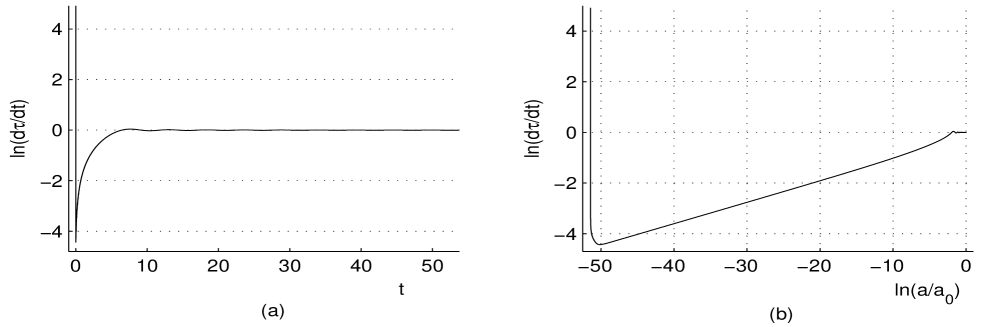
Figure 14: Typical cosmic time dependence, Fig.(a), and scale factor dependence, Fig.(b), of $\frac{d\tau}{dt}$ defined by Eq.(70) as the phase curves start from points very close to the line $Q_{1}=0$. In this figure, the initial conditions are as in Fig.12.

The $t$ and scale factor dependence of $d\tau/dt$ are presented in Fig.14. Note that the origin $t_{in}=0$ in Fig.14a is chosen just because this simplifies the numerical computations and it has no a real physical sense. After the exit from inflation, when $\phi(t)\rightarrow\phi_{0}$ (see Eq.(36)) and $\rho$ starts to fall to zero, the time coordinate $\tau$ tends to coincide with the cosmic time $t$: $d\tau/dt\rightarrow 1$. Fig.14a shows that the most of the time the coordinate $\tau$ practically coincides with the cosmic time $t$ and this happens after the exit from inflation, as one can conclude from Figs. 12 and 14b. But at the very beginning of the scenario, if the phase curve $C$ starts from a point very close to the line $Q_{1}=0$, $d\tau/dt$ is very big. In the limit $t_{in}\rightarrow t_{s}$ (where $t_{s}$ is defined in the beginning of the previous subsection), $d\tau/dt$ approaches infinity very fast such that for any $t_{1}>t_{in}$

$$\tau(t_{1})=\lim_{t_{in}\rightarrow t_{s}}\int_{t_{in}}^{t_{1}}\frac{d\tau}{dt}dt=\infty$$ (71)

By continuation of the classical solution to the past we inevitably arrive a regime where the appropriate phase curve becomes infinitely close to the line $Q_{1}=0$. If the classical evolution had started from this regime then the age of the universe will be infinite when it is measured in the natural time $\tau$. It is also interesting to see what kind of information one can obtain analytically about the behavior of the universe in this starting regime. For this let us rewrite the $\phi$-equation (22) in terms of the $\tau$ dependent $\phi$, $\dot{\phi}=Q_{1}^{-1/2}d\phi/d\tau$ and $H=\dot{a}/a=Q_{1}^{-1/2}d(\ln a)/d\tau$:

$$\frac{d^{2}\phi}{d\tau^{2}}-\left(\frac{1}{2}\frac{dQ_{1}}{d\tau}-3Q_{2}\frac{d\ln a}{d\tau}\right)\frac{1}{Q_{1}}\frac{d\phi}{d\tau}-\frac{\alpha}{2M_{p}|V_{2}|}Q_{3}M^{4}e^{-2\alpha\phi/M_{p}}=0.$$ (72)

As we know, the $\phi$-equation is regular in all points of zone I (excluding the line $Q_{1}=0$) both in terms of the cosmic time $t$ and the natural time $\tau$. Besides, the transformation (70) is also regular in zone I and it has a singularity only in points of the line $Q_{1}=0$. Since the first and the third terms in Eq.(72) are regular everywhere in zone I, the singular behavior of the factor $Q_{1}^{-1}$ in the second term as $Q_{1}\rightarrow 0$, has to be compensated by the expression in the brackets:

$$\frac{1}{2}\frac{dQ_{1}}{d\tau}-3Q_{2}\frac{d\ln a}{d\tau}\rightarrow 0\qquad\text{as}\qquad Q_{1}\rightarrow 0.$$ (73)

We are interested in the solution $a(\tau)$ corresponding to the interval of the phase curve very close to the line $Q_{1}=0$, i.e. for very small $t_{1}$ in Eq.(71). This allows to represent $Q_{2}$ in the form $Q_{2}=Q_{2}^{(0)}+{\cal O}(t_{1})$, where $Q_{2}^{(0)}$ is the value of $Q_{2}$ in the point of the line $Q_{1}=0$ nearest to the phase curve. It follows from this that in the starting regime

$$a\approx a_{in}\exp\left(\frac{Q_{1}}{6Q_{2}^{(0)}}\right),$$ (74)

where $a_{in}$ is the value of the scale factor in the beginning of the starting regime. Since according to Eq.(71) $Q_{1}$ remains extremely close to zero during indefinitely long time $\tau$, the scale factor also remains very close to $a_{in}$ for a very long time $\tau$. This may be compared with the picture addressed by the emergent universe modelsemergent where the scale factor also remains constant during indefinitely long time in the beginning. Another similar feature is that in Ref.emergent the starting regime can also be realized at an energy scale much lower the quantum Planck era. However, in contrast to the modelsemergent in our case there are no needs neither of a spatial curvature, nor of the fine tuning of the initial conditions.

VI TMT Cosmology With No Fine Tuning II:
Absence of the Initial Singularity of the Curvature and Inflationary Cosmology with Graceful Exit to a Small Cosmological Constant State

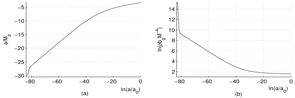
Figure 15: In the model with $\delta=0.1$, $\alpha=0.2$, $V_{1}=10M^{4}$ and $V_{2}=4b_{g}M^{4}$: (a) Typical scale factor dependence of the inflaton $\phi$ and (b) the energy density $\rho$ for the phase curves starting from points very close to the line $Q_{1}=0$ (in this figure - for $\phi_{in}=-30$, $\dot{\phi}_{in}=4540.52202M^{2}$).

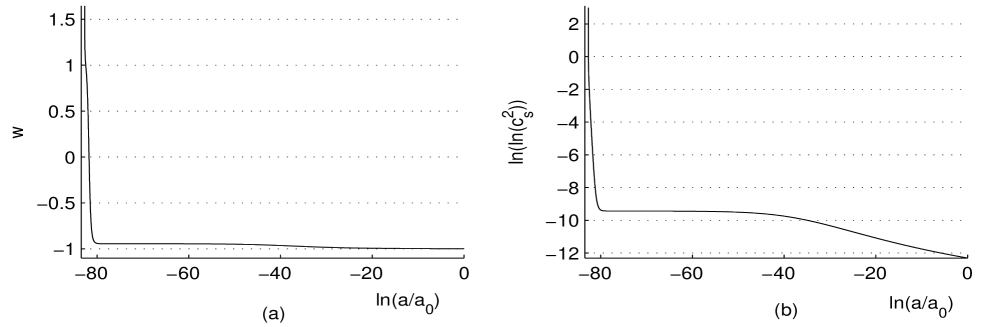
Figure 16: The same model and the same initial conditions as in Fig.15: (a) Typical scale factor dependence of $w$ and (b) the squared sound speed $c^{2}_{s}$ for the phase curves starting from points very close to the line $Q_{1}=0$.

With other choice of the parameters $V_{1}$ and $V_{2}$, but keeping the condition (47), one can realize a scenario where the pre-inflationary epoch and inflation practically coincide with those of the previous section but the exit from inflation and subsequent evolution are similar to those studied in Sec.IVC. We present here the results of numerical solutions for the model with $\delta=0.1$, $\alpha=0.2$, $V_{1}=10M^{4}$ and $V_{2}=4b_{g}M^{4}$. The structure of the phase plane, the behavior of the phase curves and the attractor are very similar to what we have seen in Figs.9 and 10, i.e zones I, II and III are present in the same manner, and for this reason we do not repeat the plane phase picture here. Therefore the same effects, namely the sudden singularity at $S_{1}=0$ and power law inflation present in this model as well. The only essential difference consists in the absence of the oscillatory regime labeled as the point $B$ in Figs.9 and 10. Now instead of this, all trajectories approach the attractor which in its turn asymptotically (as $\phi\rightarrow\infty$) takes the form of the straight line $\dot{\phi}=0$.

Typical scale factor dependence of the inflaton $\phi$, the energy density $\rho$, the equation-of-state $w$ and the sound speed of perturbations $c_{s}^{2}$ are presented in Figs.15 and 16. Their behavior in the very early universe is actually identical to that in the model of the previous section. Again, it is not a problem to obtain more than 75 e-folds during the power law inflation (the region of $w\approx-0.95$ in Fig.16a) just by choosing a larger absolute value $|\phi_{in}|$. We have chosen $\phi_{in}=-30M_{p}$ because this allows to show more details in these graphs. During the power low inflation and in the late universe the behavior of $\phi$, $\rho$ and $w$ is very similar to what we have seen in the model of Sec.IVC, see Fig.5. $c_{s}^{2}$ starting from a huge value decreases to a value slightly bigger than 1 and remains practically constant during the power low inflation; afterward it asymptotically approaches the value $c_{s}=1$.

VII TMT Cosmology With No Fine Tuning III: Superaccelerated Universe

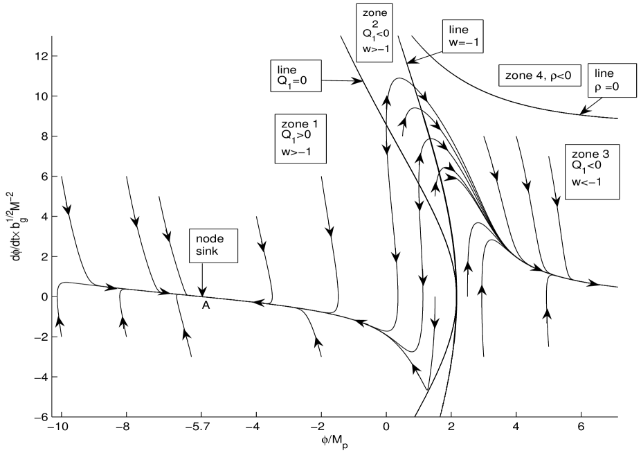
Figure 17: The phase portrait for the model with $\alpha=0.2$, $\delta=0.1$, $V_{1}=10M^{4}$ and $V_{2}=9.9b_{g}M^{4}$. The region with $\rho>0$ is divided into two dynamically disconnected regions by the line $Q_{1}(\phi,\dot{\phi})=0$. To the left of this line $Q_{1}>0$ (the appropriate zone we call zone 1) and to the right   $Q_{1}<0$. In zone 1, the phase portrait in the neighborhood of the node sink is similar to that of Sec.IVD. However the dynamical protection from initial singularities takes place here for the same reasons as those considered in Secs.V and VI. The $\rho>0$ region to the right of the line $Q_{1}(\phi,\dot{\phi})=0$ is divided into two zones (zone 2 and zone 3) by the line $Q_{2}=0$ (the latter coincides with the line where $w=-1$). In zone 2   $w>-1$ but $c_{s}^{2}<0$. In zone 3  $w<-1$ and $c_{s}^{2}>0$. Phase curves started in zone 2 cross the line $w=-1$. All phase curves in zone 3 exhibit processes with super-accelerating expansion of the universe. Besides all the phase curves in zone 3 demonstrate dynamical attractor behavior to the line which asymptotically, as $\phi\to\infty$, approaches the straight line $\dot{\phi}=0$.

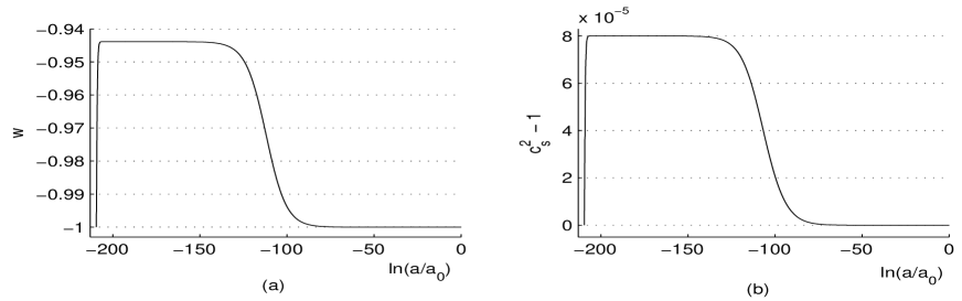
Figure 18: For the model with $\alpha=0.2$, $\delta=0.1$, $V_{1}=10M^{4}$ and $V_{2}=9.9b_{g}M^{4}$: typical scale factor dependence of the equation-of-state $w$ (Fig.(a)) and effective speed of sound for perturbations $c_{s}^{2}$ (Fig.(b)) for phase curves in zone 1 (in the figure the initial conditions are $\phi_{in}=-50M_{p}$, $\dot{\phi}_{in}=0$).

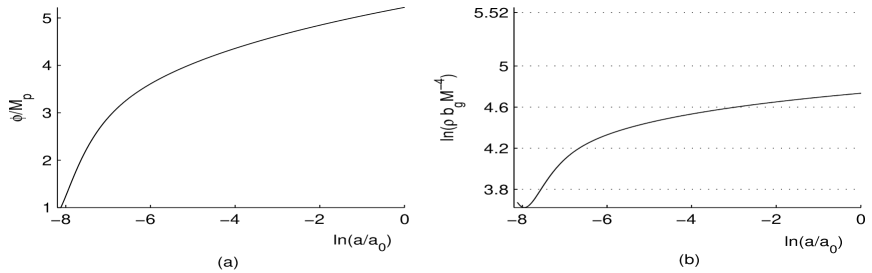
Figure 19: For the model with $\alpha=0.2$, $\delta=0.1$, $V_{1}=10M^{4}$ and $V_{2}=9.9b_{g}M^{4}$: typical scalar factor dependence of $\phi$ (Fig.(a)) and of the energy density $\rho$, defined by Eq.(20), (Fig(b)) in the regime corresponding to the phase curves started in zone 2. Both graphs correspond to the initial conditions $\phi_{in}=M_{p}$, $\dot{\phi}_{in}=5.7M^{2}/\sqrt{b_{g}}$; $\rho$ increases approaching asymptotically $\Lambda_{2}=\frac{M^{4}}{b_{g}}e^{5.52}$, where $\Lambda_{2}$ is the value of $\Lambda$ determined by Eq.(41); see also Fig.1b.

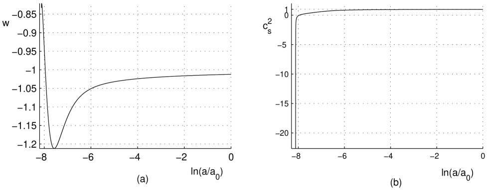
Figure 20: For the model with $\alpha=0.2$, $\delta=0.1$, $V_{1}=10M^{4}$ and $V_{2}=9.9b_{g}M^{4}$: typical scale factor dependence of the equation-of-state $w$ (Fig.(a)) and effective speed of sound for perturbations $c_{s}^{2}$ (Fig.(b)) for phase curves in zones 2 and 3 (in the figure the initial conditions are $\phi_{in}=M_{p}$, $\dot{\phi}_{in}=5.7M^{2}/\sqrt{b_{g}}$.

Equations $Q_{i}(\phi,\dot{\phi})=0$   ($i=1,2,3$)   determine lines in the phase plane $(\phi,\dot{\phi})$. In terms of a mechanical interpretation of Eq.(22), the change of the sign of $Q_{1}$ can be treated as the change of the mass of ”the particle”. Therefore one can think of situation where ”the particle” climbs up in the potential with acceleration. It turns out that when the scalar field is behaving in this way, the flat FRW universe may undergo a super-acceleration.

With simple algebra one can see that the following ”sign rule” holds for the equation-of-state $w=p/\rho$:

$$sign(w+1)=sign(Q_{2})$$ (75)

Therefore if in the one side from the line $Q_{2}(\phi,\dot{\phi})=0$   $w>-1$ then in the other side $w<-1$. To incorporate the region of the phase plane where $w<-1$ into the cosmological dynamics one should provide that the line $Q_{2}(\phi,\dot{\phi})=0$ lies in a dynamically permitted zone. As we have seen in Secs.V and VI, the condition (47) disposes the line $Q_{2}(\phi,\dot{\phi})=0$ in the physically unacceptable region where $\rho<0$. It turns out that if the opposite condition holds

$$(b_{g}+b_{\phi})V_{1}-2V_{2}<0$$ (76)

then the line $Q_{2}(\phi,\dot{\phi})=0$ may be in a dynamically permitted zone.

There are a lot of sets of parameters providing the $w<-1$ phase in the late universe. For example we are demonstrating here this effect with the following set of the parameters of the original action(9): $\alpha=0.2$, $V_{1}=10M^{4}$ and $V_{2}=9.9b_{g}M^{4}$ used in Sec.IVD but now we choose $\delta=0.1$ instead of $\delta=0$. The results of the numerical solution are presented in Figs.17-20.

The phase plane, Fig.17, is divided into two regions by the line $\rho=0$. The region $\rho>0$ is divided into two dynamically disconnected regions by the line $Q_{1}(\phi,\dot{\phi})=0$.

To the left of the line $Q_{1}(\phi,\dot{\phi})=0$ - zone 1 where $Q_{1}>0$. Comparing carefully the phase portrait in the zone 1 with that in Fig.7 of Sec.IVD, one can see an effect of $\delta\neq 0$ on the shape of phase trajectories. However the general structure of these two phase portraits is very similar. In particular, they have the same node sink $A(-5.7M_{p},0)$. At this point ”the force” equals zero since $Q_{3}|_{A}=0$. The value $\phi=-5.7M_{p}$ coincides with the position of the minimum of $V_{eff}^{(0)}(\phi)$ because in the limit $\dot{\phi}\rightarrow 0$ the role of the terms proportional to $\delta$ is negligible. Among trajectories converging to node $A$ there are also trajectories corresponding to a power low inflation of the early universe, which is just a generalization to the case $\delta\neq 0$ of the similar result discussed in Sec.IVD. For illustration we present some features of one of the solutions in Fig.18. Note that the same mechanism of the dynamical protection from the initial singularity we have discussed in Secs.V and VI, holds also here for solutions whose phase curves are located in zone 1.

In the region to the right of the line $Q_{1}(\phi,\dot{\phi})=0$, all phase curves approach the attractor which in its turn asymptotically (as $\phi\rightarrow\infty$) takes the form of the straight line $\dot{\phi}=0$. This region is divided into two zones by the line $Q_{2}(\phi,\dot{\phi})=0$. In all points of this line $w=-1$. In zone 2, i.e. between the lines $Q_{1}=0$ and $w=-1$, the equation-of-state $w>-1$ and the sound speed $c_{s}^{2}<0$. Therefore in zone 2 the model is absolutely unstable and has no any physical meaning. In zone 3, i.e. between the line $w=-1$ and the line $\rho=0$, the equation-of-state $w<-1$ and the sound speed $c_{s}^{2}>0$.

For a particular choice of the initial data $\phi_{in}=M_{p}$, $\dot{\phi}_{in}=9M^{4}/\sqrt{b_{g}}$, the features of the solution of the equations of motion are presented in Figs.19 and 20. The main features of the solution as we observe from the figures are the following: 1) $\phi$ slowly increases in time; 2) the energy density $\rho$ slowly increases approaching the constant $\Lambda=\Lambda_{2}$ defined by the same formula as in Eq.(41), see also Fig.1b; for the chosen parameters $\Lambda_{2}\approx\frac{M^{4}}{b_{g}}e^{5.52}$;  3) in zone 3 $w$ becomes less than $-1$ and after achieving a minimum $w\approx-1.2$ it then increases asymptotically approaching $-1$ from below.

Using the classification of Ref.Vikman of conditions for the dark energy to evolve from the state with $w>-1$ to the phantom state, we see that transition of the phase curves from zone 2 (where $w>-1$) to the phantom zone 3 (where $w<-1$) occurs under the conditions $p_{,X}=0$, $\rho_{,X}\neq 0$, $X\neq 0$. Qualitatively the same behavior one observes for all initial conditions $(\phi_{in},\dot{\phi}_{in})$ disposed in the zone 2. The question of constructing a realistic scenario where the dark energy can evolve from the power low inflation state disposed in zone 1 to the phantom zone 3 is beyond of the goal of this paper.

VIII Resolutions of the Cosmological Constant Problems and Connection Between TMT and Conventional Field Theories with Integration Measure $\sqrt{-g}$

VIII.1 The new cosmological constant problem

The smallness of the observable cosmological constant $\Lambda$ is known as the new cosmological constant problemWeinberg2 . In TMT, there are two ways to provide the observable order of magnitude of $\Lambda\sim(10^{-3}eV)^{4}$ by an appropriate choice of the parameters of the theory (see Eqs.(41) and (35)) but without fine tuning of the dimensionfull parameters.

VIII.1.1 Seesaw mechanism

If $V_{2}<0$ then there is no need for $V_{1}$ and $V_{2}$ to be small: it is enough that $b_{g}V_{1}<|V_{2}|$ and $V_{1}/|V_{2}|\ll 1$. This possibility is a kind of seesaw mechanismG1 ,seesaw ). For instance, if $V_{1}$ is determined by the energy scale of electroweak symmetry breaking $V_{1}\sim(10^{3}GeV)^{4}$ and $V_{2}$ is determined by the Planck scale $V_{2}\sim(10^{18}GeV)^{4}$ then $\Lambda_{1}\sim(10^{-3}eV)^{4}$. The range of the possible scale of the dimensionless parameter $b_{g}$ remains very broad.

VIII.1.2 The TMT correspondence principle and the smallness of $\Lambda$

Let us start from the notion that if $V_{2}>0$ or alternatively $V_{2}<0$ and $b_{g}V_{1}>|V_{2}|$ then $\Lambda\sim\frac{V_{1}}{b_{g}}$. Hence the second possibility to ensure the needed smallness of $\Lambda$ is to choose the dimensionless parameter $b_{g}>0$ to be a huge number. In this case the order of magnitudes of $V_{1}$ and $V_{2}$ could be either as in the above case of the seesaw mechanism or to be not too much different from each other (or even of the same order). For example, if $V_{1}\sim(10^{3}GeV)^{4}$ then for getting $\Lambda_{1}\sim(10^{-3}eV)^{4}$ one should assume that $b_{g}\sim 10^{60}$. It is important to stress that as it was explained in footnote 69, the huge value of $b_{g}$ can be equivalently regarded as an extremely small ($\sim 10^{-60}$) value of the coupling constant of the scalar curvature to the measure $\Phi$. Below we will use this value just for illustrative purposes.

Note that $b_{g}$ is the ratio of the coupling constants of the scalar curvature to the measures $\sqrt{-g}$ and $\Phi$ respectively in the fundamental action (9). The Lagrangians $L_{1}$ and $L_{2}$ have the same structure: both of them contain the scalar curvature, kinetic and pre-potential terms. It is natural to assume that the ratio of couplings of all the corresponding terms in $L_{1}$ and $L_{2}$ to the measures $\sqrt{-g}$ and $\Phi$ have the same or close orders of magnitude. This is why in Sec.III we have made an assumption that the dimensionless parameters $b_{g}$ and $b_{\phi}$ have close orders of magnitude. For the same reason we will also assume that $V_{2}/V_{1}\sim b_{g}\sim 10^{60}$. If this is the case then the huge value of $b_{g}$ can be treated as an indication that TMT implies a certain sort of the correspondence principle between TMT and conventional field theories (i.e theories with only the measure of integration $\sqrt{-g}$ in the action). In fact, using the notations of the general form of the TMT action (1) in the case of the action (9), one can conclude that the relation between the ”usual” (i.e. entering in the action with the usual measure $\sqrt{-g}$) Lagrangian density $L_{2}$ and the new one $L_{1}$ (entering in the action with the new measure $\Phi$) is roughly speaking $L_{2}\sim 10^{60}L_{1}$. In the case $\int L_{1}\Phi d^{4}x$ becomes negligible, the remaining term of the action $\int L_{2}\sqrt{-g}d^{4}x$ would describe GR instead of TMT. It seems to be very interesting that such a correspondence principle for the TMT action (1) may have a certain relation to the extreme smallness of the cosmological constant.

Appearance of a large dimensionless constant in particle field theory is usually associated with hierarchy of masses and/or interactions describing by different terms in the Lagrangian. The way large numbers can appear in the TMT action is absolutely different. It is easier to see this difference in the case of a fine tuned model, where $b_{g}=b_{\phi}$ and $b_{g}V_{1}=V_{2}$, see Appendix B. In such a case the Lagrangians $L_{1}$ and $L_{2}$ not only have the same type of terms but they are just proportional: $L_{2}=b_{g}L_{1}$. Therefore the nature of the huge value of $b_{g}$ differs here very much from the conventional hierarchy issue.

If such the ratio between $L_{1}$ and $L_{2}$ is actually realized, then taking into account the fact that $L_{1}$ and $L_{2}$ describe the same matter and gravity degrees of freedom in a very similar manner, the question arises why $L_{1}$ is not dynamically negligible in comparison with $L_{2}$. To answer this question we have to turn to the fundamental action (9) that it is convenient to rewrite in the following form

$$S= \int\sqrt{-g}d^{4}xe^{\alpha\phi/M_{p}}\left[-\frac{b_{g}}{\kappa}R(\Gamma,g)\left(\frac{\zeta}{b_{g}}+1\right)+\left(\frac{\zeta}{b_{g}}+\frac{b_{\phi}}{b_{g}}\right)\frac{b_{g}}{2}g^{\mu\nu}\phi_{,\mu}\phi_{,\nu}-e^{\alpha\phi/M_{p}}\left(\zeta\frac{V_{1}}{V_{2}}+1\right)V_{2}\right]$$ (77)

where one can see that the ratio $\zeta/b_{g}$ has an important dynamical role. Analyzing the constraint (16) and cosmological dynamics studied in Secs.IV-VI it is easy to see that the order of magnitude of the scalar field $\zeta\equiv\Phi/\sqrt{-g}$ is generically close to that of $b_{g}$ (recall that $b_{\phi}/b_{g}\sim 1$). In other words, it turns out that on the mass shell the ratio of the measures $\Phi/\sqrt{-g}$ generically compensates the smallness of $L_{1}/L_{2}$. Thus, similar terms ($R$-terms, kinetic terms and pre-potential terms) appearing in the action (9) with measures $\Phi$ and $\sqrt{-g}$ respectively, are both dynamically important in general.

In the light of this understanding of the general picture it is interesting to check the TMT dynamics in situations where $\zeta/b_{g}$ becomes very small. Let us start from the fine tuned model where $b_{g}V_{1}=2V_{2}$ and $b_{g}=b_{\phi}$ (recall that $b_{g}>0$ and we consider the case $V_{1}>0$). In this case it follows from the constraint (31) that

$$\frac{\zeta}{b_{g}}=\frac{M^{4}e^{-2\alpha\phi/M_{p}}}{V_{1}+M^{4}e^{-2\alpha\phi/M_{p}}},$$ (78)

Then the effective potential (33) (see also Eqs.(40)-(42)) reads

$$V_{eff}^{(0)}(\phi)=\frac{V_{2}}{b_{g}^{2}}+\frac{M^{8}e^{-4\alpha\phi/M_{p}}}{2b_{g}(V_{1}+2M^{4}e^{-2\alpha\phi/M_{p}})}.$$ (79)

In such a fine tuned model, $\zeta/b_{g}$ approaches zero asymptotically as $\phi\rightarrow\infty$ where the effective potential becomes flat. However when looking into the TMT action written in the form (77) we see that the asymptotic disappearance of $\zeta/b_{g}$ means that we deal with an asymptotic transition from TMT to a conventional field theory model with only measure of integration $\sqrt{-g}$ and only one Lagrangian density. In the limit $\zeta/b_{g}\rightarrow 0$, the transformation to the Einstein frame (10) takes the form $\tilde{g}_{\mu\nu}=b_{g}e^{\alpha\phi/M_{p}}g_{\mu\nu}$. Therefore in the Einstein frame, the limit of the action (77) as $\zeta/b_{g}\rightarrow 0$ is reduced to the following model:

$$S|_{\zeta=0,\,Eistein\,frame}=\int\sqrt{-\tilde{g}}d^{4}x\left[-\frac{1}{\kappa}R(\tilde{g})+\frac{1}{2}\tilde{g}^{\mu\nu}\phi_{,\mu}\phi_{,\nu}-\frac{1}{b_{g}^{2}}V_{2}\right].$$ (80)

It is easy to see that for example in the FRW universe, the asymptotic (as the scale factor $a(t)\rightarrow\infty$) behavior of the universe in the model (80) coincides with the appropriate asymptotic result of TMT model under consideration: both of them asymptotically describe the universe governed by the cosmological constant $V_{2}/b_{g}^{2}=V_{1}/2b_{g}$.

Similar conclusion is obtained in a model where $V_{2}<b_{g}V_{1}<2V_{2}$, i.e. with no fine tuning of the prepotentials, which have been studied in Sec.IVD. The only difference is that now $\zeta/b_{g}\rightarrow 0$ and $V_{eff}\rightarrow V_{2}/b_{g}^{2}\sim V_{1}/b_{g}$ as $\phi\rightarrow\phi_{min}$, see Eq.(43); in a small neighborhood of $\phi_{min}$ the TMT action presented in the Einstein frame looks like (80).

Note however that in the context of the k-essence model studied in Sec.VII where $\delta\neq 0$ and $V_{2}<b_{g}V_{1}<2V_{2}$, the asymptotic value of $\zeta$ in the late time universe ( as $\phi\rightarrow\infty$ and $X\rightarrow 0$ which is an asymptotic regime of the phantom behavior) is $|\zeta|\sim b_{g}$ but nevertheless the energy density tends to $\Lambda=\Lambda_{2}=\frac{V_{1}^{2}}{4(b_{g}V_{1}-V_{2})}\sim V_{1}/b_{g}$ as well (see Figs.1b and 19b).

Similar situation takes place in the model where $b_{g}V_{1}>2V_{2}$, studied in Secs.IVC and VI. The asymptotic value of $\zeta$ in the late time universe is again $\zeta\sim b_{g}$ and the energy density tends to $\Lambda=\Lambda_{1}=\frac{V_{1}^{2}}{4(b_{g}V_{1}-V_{2})}\sim V_{1}/b_{g}$ as well (see Figs.1a, 5b and 15b).

Thus in all the models, the huge value of $b_{g}$ can ensure the needed smallness of the dark energy density in the late time universe but it is not always realized due to the limit $\zeta/b_{g}\rightarrow 0$.

VIII.2 The Old Cosmological Constant Problem Is Solved in the Dynamical Regime where the Fundamental TMT Action Tends to a Limit Opposite to Conventional Field Theory (with only measure $\sqrt{-g}$).

As we have seen in Sec.IVB, in the model with $V_{1}<0$ and $V_{2}<0$, the old cosmological constant problem is resolved without fine tuning: the effective potential (33) is proportional to the square of $V_{1}+M^{4}e^{-2\alpha\phi/M_{p}}$, and $\phi=\phi_{0}$ where $V_{1}+M^{4}e^{-2\alpha\phi_{0}/M_{p}}=0$, is the minimum of the effective potential without any further tuning of the parameters and initial conditions. Now we want to analyze some of the essential differences we have in TMT as compared with the conditions of the Weinberg’s no-go theorem and show what are the reasons providing solution of the old CC problem in TMT. This has to be done when TMT is considered in the original frame since in the Einstein frame we observe only the results in the effective picture after some of the symmetries are broken.

• The basic assumption of the Weinberg’s theorem is that in the vacuum all the fields (metric tensor $g_{\mu\nu}$ and matter fields $\psi_{n}$) are constant. As it was pointed out by S.Weinberg in the reviewWeinberg1 , the Euler-Lagrange equations for such constant fields (with the action $\int{\cal L}\left(g_{\mu\nu},\psi_{n}\right)d^{4}x$) have the form

  $$\frac{\partial{\cal L}}{\partial g_{\mu\nu}}=0,$$ (81)

  $$\frac{\partial{\cal L}}{\partial\psi_{n}}=0$$ (82)

  and these equations constitute the basis for further Weinberg’s arguments. In particular, if $GL(4)$ symmetry

  $$g_{\mu\nu}\rightarrow A^{\alpha}_{\mu}A^{\beta}_{\nu}g_{\alpha\beta},\qquad\psi_{i}\rightarrow D_{ij}(A)\psi_{j}$$ (83)

  survives as a vestige of general covariance when all the fields are constrained to be constant, the Lagrangian ${\cal L}$ transforms as a density:

  $${\cal L}\rightarrow detA\cdot{\cal L}.$$ (84)

  Weinberg concludes that when Eq.(81) is satisfied then the unique form of ${\cal L}$ is

  $${\cal L}=c\sqrt{-g},$$ (85)

  where $c$ is independent of $g_{\mu\nu}$. As a matter of fact this means that for example in the case of a scalar matter field $\phi$ model considered by Weinberg in Sec.VI of the review Weinberg1 , $c$ is determined by the value of the scalar field $\phi$ potential as $\phi$ is a constant determined by Eq.(82).

  However, if for example one of the fields $\psi_{n}$ appears in ${\cal L}$ only via a term linear in space-time derivatives of this field then Eq.(82) turns out to be an identity, but instead the Euler-Lagrange equations take another form. This is what happens in TMT where the first term in the action (1) is linear in space-time derivatives of $A_{\alpha\beta\gamma}$ (when using the definition (3))(see also ). Then instead of Eq.(82) which appears to be an identity in this case, the Euler-Lagrange equations for $A_{\alpha\beta\gamma}$ look

  $$\partial_{\mu}\frac{\partial({\Phi L_{1}})}{\partial A_{\alpha\beta\gamma,\mu}}=0,$$ (86)

  which are nontrivial even for constant $A_{\alpha\beta\gamma}$, and resulting in Eq.(6). Note that $\Phi L_{1}$ is a scalar density and transforms exactly according to Eq.(84). Therefore generically (i.e. if $A_{\alpha\beta\gamma}$ are not constant while other fields are constant), the Lagrangian ${\cal L}$ satisfying (84) can have the following form

  $${\cal L}=c_{1}\Phi+c_{2}\sqrt{-g}$$ (87)

  where $c_{1}$ and $c_{2}$ are independent of $g_{\mu\nu}$ and $\Phi$. This is why the equation

  $$\partial{\cal L}/\partial\phi=T^{\mu}_{\mu}\sqrt{-g},$$ (88)

  where $T^{\mu}_{\mu}$ is the trace of the energy-momentum tensor, used by WeinbergWeinberg1 for all constant $g_{\mu\nu}$ and matter fields, is generically no longer valid.

• Let us now note that $\zeta=\zeta_{0}(\phi)$, Eq.(31), becomes singular

  $$|\zeta|\approx\frac{2|V_{2}|}{|V_{1}+M^{4}e^{-2\alpha\phi/M_{p}}|}\rightarrow\infty\qquad\text{as}\qquad\phi\rightarrow\phi_{0}.$$ (89)

  In this limit the effective potential (14) (see also Eq.(33)) behaves as

  $$V_{eff}\approx\frac{|V_{2}|}{\zeta^{2}}.$$ (90)

  Thus, disappearance of the cosmological constant occurs in the regime where $|\zeta|\rightarrow\infty$. In this limit, the dynamical role of the terms of the Lagrangian $L_{2}$ (coupled with the measure $\sqrt{-g}$) in the action (9) becomes negligible in comparison with the terms of the Lagrangian $L_{1}$ (see also the general form of the action (1)). A particular realization of this we observe in the behavior of $V_{eff}$, Eq.(90). It is evident that the limit of the TMT action (1) as $|\zeta|\rightarrow\infty$ is opposite to the conventional field theory (with only measure $\sqrt{-g}$) limit of the TMT action discussed in subsection VIIIA. From the point of view of TMT, this is the answer to the question why the old cosmological constant problem cannot be solved (without fine tuning) in theories with only the measure of integration $\sqrt{-g}$ in the action.

• Recall that one of the basic assumptions of the Weinberg’s no-go theorem is that all fields in the vacuum must be constant. This is also assumed for the metric tensor, components of which in the vacuum must be nonzero constants. However, this is not the case in the fundamental TMT action (9) defined in the original (non Einstein) frame if we ask what is the metric tensor $g_{\mu\nu}$ in the $\Lambda=0$ vacuum . To see this let us note that in the Einstein frame all the terms in the cosmological equations are regular. This means that the metric tensor in the Einstein frame $\tilde{g}_{\mu\nu}$ is always well defined, including the $\Lambda=0$ vacuum state $\phi=\phi_{0}$ where $\zeta$ is infinite. Taking this into account and using the transformation to the Einstein frame (10) we see that all components of the metric in the original frame $g_{\mu\nu}$ go to zero overall in space-time as $\phi$ approaches the $\Lambda=0$ vacuum state:

  $$g_{\mu\nu}\sim\frac{1}{\zeta}\sim V_{1}+M^{4}e^{-2\alpha\phi/M_{p}}\rightarrow 0\qquad(\mu,\nu=0,1,2,3)\qquad\text{as}\quad\phi\rightarrow\phi_{0}.$$ (91)

  This result shows that the Weinberg’s analysis based on the study of the trace of the energy-momentum tensor misses any sense in the case $g_{\mu\nu}=0$.

  The metric is an attribute of the space-time term. Hence disappearance of the metric $g_{\mu\nu}$ in the limit $\phi\rightarrow\phi_{0}$ means that the strict formulation of the TMT model (9) with $V_{1}<0$ and $V_{2}<0$ may require a new mathematical basis. A manifold which is not equipped with the metric (corresponding to the $\Lambda=0$ vacuum state) emerges as a certain limit of a sequence of space-times. Thus the model under consideration might be formulated not in a space-time manifold but rather by means of a set of space-time manifolds. A limiting point of a sequence of space-times is a ”vacuum space-time manifold” one of the differences of which from a regular space-time consists in the absence of the metric $g_{\mu\nu}$.

  It follows immediately from (91) that $\sqrt{-g}$ tends to zero like

  $$\sqrt{-g}\sim\frac{1}{\zeta^{2}}\sim\left(V_{1}+M^{4}e^{-2\alpha\phi/M_{p}}\right)^{2}\rightarrow 0\quad\text{as}\quad\phi\rightarrow\phi_{0}.$$ (92)

  Then the definition $\zeta\equiv\Phi/\sqrt{-g}$ implies that the integration measure $\Phi$ also tends to zero but rather like

  $$\Phi\sim\frac{1}{\zeta}\sim V_{1}+M^{4}e^{-2\alpha\phi/M_{p}}\rightarrow 0\quad\text{as}\quad\phi\rightarrow\phi_{0}.$$ (93)

  Thus both the measure $\Phi$ and the measure $\sqrt{-g}$ become degenerate in the $\Lambda=0$ vacuum state $\phi=\phi_{0}$. However $\sqrt{-g}$ tends to zero more rapidly than $\Phi$.

• As we have discussed in detail (see Secs.II, IIIB and Refs.GK2 ,GK3 ), with the original set of variables used in the fundamental TMT action it is very hard or may be even impossible to display the physical meaning of TMT models. One of the reasons is that in the framework of the postulated need to use the Palatini formalism, the original metric $g_{\mu\nu}$ and connection $\Gamma^{\alpha}_{\mu\nu}$ appearing in the fundamental TMT action describe a non-Riemannian space-time. The transformation to the Einstein frame (10) enables to see the physical meaning of TMT because the space-time becomes Riemannian in the Einstein frame. Now we see that the transformation to the Einstein frame (10) plays also the role of a regularization of the space-time metric: the singular behavior of the transformation (10) as $\phi\approx\phi_{0}$ compensates the disappearance of the original metric $g_{\mu\nu}$ in the vacuum $\phi=\phi_{0}$. As a result of this the metric in the Einstein frame $\tilde{g}_{\mu\nu}$ turns out to be well defined in all physical states including the $\Lambda=0$ vacuum state.

IX Discussion and Conclusion

IX.1 Differences of TMT from the standard field theory in curved space-time

The main idea of TMT is that the general form of the action $\int L\sqrt{-g}d^{4}x$ is not enough in order to account for some of the fundamental problems of particle physics and cosmology. The key difference of TMT from the conventional field theory in curved space-time consists in the hypothesisGK2 -GKatz that in addition to the term in the action with the volume element $\sqrt{-g}d^{4}x$ there should be one more term where the volume element is metric independent but rather it is determined either by four (in the 4-dimensional space-time) scalar fields $\varphi_{a}$ or by a three index potential $A_{\alpha\beta\gamma}$, see Eqs.(1)-(3). We would like to emphasize that including in the action of TMT the coupling of the Lagrangian density $L_{1}$ with the measure $\Phi$, we modify in general both the gravitational and matter sectors as compared with the standard field theory in curved space-time. Besides we made two more assumptions: the measure fields ($\varphi_{a}$ or $A_{\alpha\beta\gamma}$) appear only in the volume element; one should proceed in the first order formalism. These assumptions constitute all the modifications of the general structure of the theory we have made as compared with the conventional field theory where only the measure of integration $\sqrt{-g}$ is used in the action principle. In fact, the Lagrangian densities $L_{1}$ and $L_{2}$ studied in the present paper, contain only such terms which should be present in a conventional model with minimally coupled to gravity scalar field. In particular there is no need for the non-linear kinetic term as well as for the phantom type term in the fundamental Lagrangian densities $L_{1}$ and $L_{2}$ in order to obtain a super-acceleration phase at the late time universe.

After making use of the variational principle and formulating the resulting equations in the Einstein frame, we have seen that the effective action (28) represents a concrete realization of the $k$-essencek-essence obtained from first principles of TMT without any exotic terms in the fundamental Lagrangian densities.

IX.2 Short summary of results

IX.2.1 The classical pre-inflation epoch of very early universe: absence of initial singularity of the curvature.

As $\delta=0$, i.e. in the fine-tuned model, the dynamics of $\phi$ can be analyzed by means of its effective potential (33). As $\phi\ll-M_{p}$ the effective $\phi$ potential has the exponential form and it is proportional to the integration constant $M^{4}$. In other words, the effective potential governing the dynamics of the early universe results from the spontaneous breakdown of the global scale invariance (8) caused by the intrinsic feature of TMT (see Eqs. (5) and (94)). We have seen that independently of the values of the parameters $V_{1}$, $V_{2}$ and under very general initial conditions, solutions rapidly achieve a regime of the well explored power law inflation. In this fine-tuned case the initial singularity is present in the usual senseBorde-Vilenkin-PRL .

If $\delta\neq 0$, we deal with the intrinsically $k$-essence dynamics. Here solutions also rapidly achieve a regime of power law inflation. However the solutions describing the pre-inflationary stage cannot be continued into the past till the singularity of the curvature. The reason is that the specific structure of the phase plane (when $\delta\neq 0$) does not allow classical evolution for which the phase curve crosses the line $Q_{1}(\phi,\dot{\phi})=0$ (on this line $\ddot{\phi}$ becomes infinite). Independently of how close is the starting point to the border line $Q_{1}=0$ in zone I (where $Q_{1}>0$, see Figs. 9 and 10), duration of the cosmic time evolution from the start up to the transition to the regime of the power law inflation is finite. This result takes place for all finite initial conditions $\phi_{in}$, $\dot{\phi}_{in}$ in zone I. However the energy density $\rho$, pressure $p$, the first two derivatives of the scale factor $\dot{a}$ and $\ddot{a}$ (and therefore curvature) remain finite on the line $Q_{1}(\phi,\dot{\phi})=0$ while only $\dot{p}$ and $\dddot{a}$ (and therefore time derivative of the curvature) become singular. It is clear that this type of ”sudden” singularity studied by BarrowBarrow1 on purely kinematic grounds has no relation to the initial singularity theoremsBorde-Vilenkin-PRL . Note also that the strong energy condition holds on the line $Q_{1}(\phi,\dot{\phi})=0$.

It is worthwhile to pay attention to the fact that the sound speed $c_{s}^{2}$ tends to infinity as the starting point $(\phi_{in},\dot{\phi}_{in})$ approaches the line $Q_{1}(\phi,\dot{\phi})=0$. Therefore generation of any mode of scalar fluctuations in states extremely close to the line $Q_{1}=0$ requires extremely large energy. Thus the initial state formed in the close neighborhood of the line $Q_{1}=0$ must be practically the ground state. This allows to hope that the effect $c_{s}^{2}\to\infty$ could help to solve the problem of the initial conditions in inflationary cosmology.

IX.2.2 Graceful exit from inflation

In our toy model there are three regions of the parameters $V_{1}$ and $V_{2}$ and corresponding three shapes of the effective potentials, Fig.1. Consequently three different types of scenarios for exit from inflation can be realized (note that when the kinetic term $X$ becomes small, the terms where $\delta$ appears are negligible):

a) $V_{1}<0$ and $V_{2}<0$,   Sec.IVB. In this case the power law inflation ends with damped oscillations of $\phi$ approaching the point of the phase plane ($\phi=\phi_{0},\dot{\phi}=0$) where the vacuum energy $V_{eff}^{(0)}(\phi_{0})=0$. This occurs without fine tuning of the parameters and the initial conditions.

b) $V_{1}>0$ and $b_{g}V_{1}>2V_{2}$,   Sec.IVC. In this case the power law inflation monotonically transforms to the late time inflation asymptotically governed by the cosmological constant $\Lambda_{1}$.

c) $V_{2}<b_{g}V_{1}<2V_{2}$,   Sec.IVD. In this case the power law inflation ends without oscillations at the final value $\phi_{min}$, corresponding to the (non zero) minimum of the effective potential.

The model we have studied in this paper may be extended by including the Higgs field, as well as gauge fields and fermions. It turns out that the scalar sector of such an extended model enables a scenariohep-th/0603150 which resembles a hybrid inflationhybrid . These results will be presented in a future publication.

IX.2.3 Cosmological constant problems

1) The old cosmological constant problem. In Sec.IVB we have seen in details that if $V_{1}<0$ then, for a broad range of other parameters, the vacuum energy turns out to be zero without fine tuning. This effect is a direct consequence of the TMT structure which yields the following results: a) the effective scalar field potential generated in the Einstein frame is proportional to a perfect square of a $\phi$-depending expression, which gets zero at some value of $\phi$; b) one of the terms in this expression is proportional to the integration constant $\pm M^{4}$ the appearance of which is also the intrinsic feature of TMT. If such type of the structure for the scalar field potential in a conventional (non TMT) model would be chosen ”by hand” it would be a sort of fine tuning. Note that the spontaneously broken global scale invariance is not necessary to achieve this effectGK3 .

In Sec.VIIIB we have explained in details how this result avoids the well known no-go theorem by WeinbergWeinberg1 stating that generically in field theory one cannot achieve zero value of the potential in the minimum without fine tuning. It is interesting that the resolution of the old CC problem in the context of TMT happens in the regime where $\zeta\rightarrow\infty$. From the point of view of TMT, the latter is the answer to the question why the old cosmological constant problem cannot be solved (without fine tuning) in theories with only the measure of integration $\sqrt{-g}$ in the action.

2) The new cosmological constant problem. Interesting result following from the general structure of the scale invariant TMT model with $V_{1}>0$ is that the cosmological constant $\Lambda$, Eq.(41), is a ratio of quantities constructed from pre-potentials $V_{1}$, $V_{2}$ and the dimensionless parameter $b_{g}$. Such structure of $\Lambda$ allows to propose two ways (see Sec.VIIIA) for the resolution of the problem of the smallness of $\Lambda$ that should be $\Lambda\sim(10^{-3}eV)^{4}$:

a) The first way is a kind of a seesaw mechanismseesaw . For instance, if $V_{1}\sim(10^{3}GeV)^{4}$ and $V_{2}\sim(10^{18}GeV)^{4}$ then $\Lambda_{1}\sim(10^{-3}eV)^{4}$.

b) The second way is realized if the dimensionless parameters $b_{g}$, $b_{\phi}$ and $V_{2}/V_{1}$ of the action (9) are huge numbers of the close orders of magnitude. For example, if $V_{1}\sim(10^{3}GeV)^{4}$ then for getting $\Lambda\sim(10^{-3}eV)^{4}$ one should assume that $b_{g}\sim 10^{60}$. The latter means that the ratio of the Lagrangian density $L_{1}$ coming into the underlying action with the ’new’ measure $\Phi$, to the Lagrangian density $L_{2}$ coming with the ’usual’ measure $\sqrt{-g}$, is extremely small: $L_{1}/L_{2}\sim 10^{-60}$. Possibility of this idea means that the resolution of the new cosmological constant problem may have a certain relation to the correspondence principle between TMT and conventional field theories (see details in Sec.VIII.A.2).

IX.2.4 Super-acceleration phase of the Universe.

If no fine tuning of the parameters is made in the fundamental action, namely if $b_{g}\neq b_{\phi}$, then our TMT model has big enough regions in the parameter space where the super-acceleration phase in the late time universe becomes possible. The appropriate phantom dark energy asymptotically approaches a cosmological constant. However, in the framework of our model it is impossible to obtain a pure classical solution which connects the early universe power law inflation with the late time super-acceleration. This problem is apparently related with the toy character of our TMT model. First, possible dependence of $V_{1}$ and $V_{2}$ on the Higgs field has not been taken into account. Second, the role of the matter creation has been ignored: in TMT the fermionic matter generically contributes to the constraint equation for the scalar field $\zeta$ and so can effect the field $\phi$ dynamics as well. One can speculate that matter creation at the end of inflation may cause a ’phase transition’ from the structure of the phase plane of the type shown in Figs.9 and 10 to the structure as in Fig.17. Then without any fine tuning, a scenario involving a start from finite curvature, a power law inflation in the early universe and super-accelerated late universe with small asymptotic CC would be possible.

IX.3 What can we expect from quantization

In this paper we have studied only classical TMT and its possible effects in the context of cosmology. However quantization of TMT as well as influence of quantum effects on the processes explored in this paper may have a crucial role. We summarize here some ideas and speculations which gives us a hope that quantum effects can keep the main results of this paper.

Recall first two fundamental facts of TMT as a classical field theory: (a) The measure degrees of freedom appear in the equations of motion only via the scalar $\zeta$, Eq.(7); (b) The scalar $\zeta$ is determined (as a function of matter fields, in our toy model - as a function of $\phi$) by the constraint which is nothing but a consistency condition of the equations of motion (see Eqs.(94)-(96) in Appendix A and Eq.(16)). Therefore the constraint plays a key role in TMT. Note however that if we were ignore the gravity from the very beginning in the action (9) then instead of the constraint (96) we would obtain Eq.(94) (where one has to put zero the scalar curvature). In such a case we would deal with a different theory. This notion shows that the gravity and matter intertwined in TMT in a much more complicated manner than in GR. Hence introducing the new measure of integration $\Phi$ we have to expect that the quantization of TMT may be a complicated enough problem. Nevertheless we would like here to point out that in the light of the recently proposed idea of Ref.Giddings , the incorporation of four scalar fields $\varphi_{a}$ together with the scalar density $\Phi$, Eq.(2), (which in our case are the measure fields and the new measure of integration respectively), is a possible way to define local observables in the local quantum field theory approach to quantum gravity. We regard this result as an indication that the effective gravity $+$ matter field theory has to contain the new measure of integration $\Phi$ as it is in TMT.

The assumption that the measure fields $\varphi_{a}$ (or $A_{\alpha\beta\gamma}$) appear in the action (1) only via the measure of integration $\Phi$, has a key role in the TMT results and in particular for the resolution of the old cosmological constant problem. In principle one can think of breakdown of such a structure by quantum corrections. However, TMT possesses an infinite dimensional symmetry mentioned in item 2 of Sec.II which, as we hope, is able to protect this feature of the structure of the action from a deformation caused by quantum corrections. Another effect of quantum corrections is the possible appearance of a nonminimal coupling of the scalar field $\phi$ to gravity in the form like for example $\xi R\phi^{2}$. Proceeding in the first order formalism of TMT one can show that the nonminimal coupling can affect the k-essence dynamics but the mechanism for resolution of the old CC problem exhibited in this paper remains unchanged. This conclusion together with expected effect of quantum corrections on the scale invariance, including appearance of a ”normal” cosmological constant term $\int\tilde{\Lambda}\sqrt{-g}d^{4}x$ (see our discussion in the paragraph after Eq.(36)), allows us to hope that the quantization of the underlying TMT model (9) will not spoil the exhibited resolution of the old CC problem.

Quantization of TMT being a constrained system requires developing the Hamiltonian formulation of TMT. Preliminary consideration shows that the Einstein frame appears in the canonical formalism in a very natural manner. A systematic exploration of TMT in the canonical formalism will be a subject of forthcoming research.

IX.4 Possible quantum effects on the initial singularity related to the line $Q_{1}=0$

Possibility of the classical evolution of the universe to start from finite values of $\rho_{in}$, $p_{in}$ such that $\dot{a}_{in}$ and $\ddot{a}_{in}$ are finite and $Q_{1}(\phi_{in},\dot{\phi}_{in})\approx 0$, requires certain arguments addressed to explain how such an initial state could be formed.

One can think of the action (9) of the underlying model as a tree approximation of the entire TMT effective action at energies below the Planck scale. Then one can expect that the next terms in the expansion of the entire effective action will be like $R^{2}(\Gamma,g)$, $(g^{\mu\nu}\phi_{,\mu}\phi_{,\nu})^{2}$ etc. coupled both to the measure $\sqrt{-g}$ and to the measure $\Phi$. It is evident that in such more general TMT model formulated in the Einstein frame, the $X$ dependence of the matter Lagrangian density $p(\phi,X;M)$ in Eq.(28) may be very much different from that in Eq.(21). As a result of this the structure of the phase plane may change quantitatively in comparison with that of the model studied in the present paper. For example, it may be found that the new factor $Q_{1}(\phi,\dot{\phi};M)$ has no zeros. In such a case the effect of the initial singularity related to the line $Q_{1}=0$ vanishes. However this is only one of the possibilities. In the absence of a reliable knowledge about the entire effective action one can also expect, with not less grounds, that the changed structure of the phase plane still involves the line $Q_{1}=0$. So we return the problem formulated in the previous paragraph. At the qualitative level we can suggest the following two ideas.

1. As we have already mentioned after Eq.(68) the described initial state can be realized at the energy density close to the Planck scale. In this case, similar to the cosmological models in the framework of the standard Einstein gravity, there is a need to use the quantum gravity and therefore the singularity effects related to the line $Q_{1}=0$ are expected to be smoothed out.

2. If $\rho_{in}<\rho_{Planck}$, then quantum effects from the scalar field dynamics itself can play a crucial role in smoothing the singularity related to the line $Q_{1}=0$. Recall that $c_{s}^{2}<0$ in the regions between $Q_{1}=0$ and $\rho=0$ (where $Q_{1}<0$, see Figs.9 and 10), which means that from this side of the line $Q_{1}=0$ arbitrarily small scalar field fluctuation is amplified exponentially. Besides $c_{s}^{2}\to-\infty$ when approaching the line $Q_{1}=0$ from this side. Therefore we expect that the classical or quantum chaos in the regions with $Q_{1}<0$ should affect the classical dynamics on the other side of the border, i.e. in the close neighborhood of the line $Q_{1}=0$ in zone I. Moreover, this influence can work as a mechanism responsible for creation of our universe starting from an excitation in zone with $Q_{1}<0$.

X Acknowledgements

We acknowledge L. Amendola, S. Ansoldi, R. Barbieri, J. Bekenstein, A. Buchel, A. Dolgov, A. Feinstein, S.B. Giddings, V. Goldstein, P. Gondolo, A. Guth, B-L. Hu, P.Q. Hung, D. Kazanas, Y. Lyubarski, D. Marolf, D.G. McKeon, J. Morris, V. Miransky, H. Nielsen, Y.Jack Ng, H. Nishino, E. Nissimov, S. Pacheva, L. Parker, R. Peccei, M. Pietroni, S. Rajpoot, R. Rosenfeld, V. Rubakov, J. Senovilla, E. Spallucci, A. Vikman, A. Vilenkin, M. Visser, S. Wetterich, F. Wilczek and A. Zee for helpful conversations and communications on different stages of this research. Our special gratitude to L. Prigozhin for his help in the implementation of numerical solutions.

Appendix A Equations of motion in the original frame

Variation of the measure fields $\varphi_{a}$ with the condition $\Phi\neq 0$ leads, as we have already seen in Sec.II, to the equation $L_{1}=sM^{4}$ where $L_{1}$ is now defined, according to Eq. (1), as the part of the integrand of the action (9) coupled to the measure $\Phi$. Equation (5) in the context of the model (9) reads (with the choice $s=+1$):

$$\left[-\frac{1}{\kappa}R(\Gamma,g)+\frac{1}{2}g^{\mu\nu}\phi_{,\mu}\phi_{,\nu}\right]e^{\alpha\phi/M_{p}}-V_{1}e^{2\alpha\phi/M_{p}}=M^{4},$$ (94)

It can be noticed that the appearance of a nonzero integration constant $M^{4}$ spontaneously breaks the scale invariance (8).

Variation of the action (9) with respect to $g^{\mu\nu}$ yields

$$-\frac{1}{\kappa}(\zeta+b_{g})R_{\mu\nu}(\Gamma)+(\zeta+b_{\phi})\frac{1}{2}\phi_{,\mu}\phi_{,\nu}+\frac{1}{2}g_{\mu\nu}\left[\frac{b_{g}}{\kappa}R(\Gamma,g)-\frac{b_{\phi}}{2}g^{\alpha\beta}\phi_{,\alpha}\phi_{,\beta}+V_{2}e^{\alpha\phi/M_{p}}\right]=0.$$ (95)

We see that in contrast to field theory models with only the measure $\sqrt{-g}$, in TMT there are two independent equations containing curvature. Contracting Eq.(95) with $g^{\mu\nu}$ and solving Eq.(94) for $R(\Gamma,g)$ we obtain the following consistency condition of these two equations:

$$(\zeta-b_{g})\left(M^{4}e^{-\alpha\phi/M_{p}}+V_{1}e^{\alpha\phi/M_{p}}\right)+2V_{2}e^{\alpha\phi/M_{p}}+(b_{g}-b_{\phi})\frac{1}{2}g^{\mu\nu}\phi_{,\mu}\phi_{,\nu}=0,$$ (96)

that we will call the constraint in the original frame.

It follows from Eqs.(94) and (95) that

$$\frac{1}{\kappa}R_{\mu\nu}(\Gamma) = \frac{\zeta+b_{\phi}}{\zeta+b_{g}}\cdot\frac{1}{2}\phi_{,\mu}\phi_{,\nu}$$ (97)

$$- \frac{g_{\mu\nu}}{2(\zeta+b_{g})}\left[b_{g}M^{4}e^{-\alpha\phi/M_{p}}+(b_{g}V_{1}-V_{2})e^{\alpha\phi/M_{p}}-(b_{g}-b_{\phi})\frac{1}{2}g^{\alpha\beta}\phi_{,\alpha}\phi_{,\beta}\right]$$

The scalar field $\phi$ equation of motion in the original frame can be written in the form

$$\frac{1}{\sqrt{-g}}\partial_{\mu}\left[e^{\alpha\phi/M_{p}}(\zeta+b_{\phi})\sqrt{-g}g^{\mu\nu}\partial_{\nu}\phi\right]$$ (98)

$$- \frac{\alpha}{M_{p}}e^{\alpha\phi/M_{p}}\left[(\zeta+b_{g})M^{4}e^{-\alpha\phi/M_{p}}+[(b_{g}-\zeta)V_{1}-2V_{2}]e^{\alpha\phi/M_{p}}-(b_{g}-b_{\phi})\frac{1}{2}g^{\alpha\beta}\phi_{,\alpha}\phi_{,\beta}\right]=0$$

where Eq.(94) has been used.

Variation of the action (9) with respect to the connection degrees of freedom leads to the equations we have solved earlierGK3 . The result is

$$\Gamma^{\lambda}_{\mu\nu}=\{^{\lambda}_{\mu\nu}\}+\frac{1}{2}(\delta^{\alpha}_{\mu}\sigma,_{\nu}+\delta^{\alpha}_{\nu}\sigma,_{\mu}-\sigma,_{\beta}g_{\mu\nu}g^{\alpha\beta})$$ (99)

where $\{^{\lambda}_{\mu\nu}\}$ are the Christoffel’s connection coefficients of the metric $g_{\mu\nu}$ and

$$\sigma,_{\mu}\equiv\frac{\alpha}{M_{p}}\phi,_{\mu}+\frac{1}{\zeta+b_{g}}\zeta,_{\mu}$$ (100)

Appendix B Asymmetry between early and late time dynamics of the universe as result of asymmetry in the couplings to measures $\Phi$ and $\sqrt{-g}$ in the action.

The results obtained in Secs.IV and V depend very much on the choice of the parameters $V_{1}$, $V_{2}$ and $\delta$ in the action (9). Let us recall that the curvature term in the action (9) couples to the measure $\Phi+b_{g}\sqrt{-g}$ while the $\phi$ kinetic term couples to the measure $\Phi+b_{\phi}\sqrt{-g}$. This is the reason of $\delta\neq 0$. If we were choose the fine tuned condition $\delta=0$ then both the curvature term and the $\phi$ kinetic term would be coupled to the same measure $\Phi+b_{g}\sqrt{-g}$. One can also pay attention that depending on the choice of one of the alternative conditions $b_{g}V_{1}>2V_{2}$ or $b_{g}V_{1}<2V_{2}$ we realize different shapes of the effective potential if $b_{g}V_{1}>V_{2}$ (see Fig.1). And again, if instead we were choose the fine tuned condition $b_{g}V_{1}=V_{2}$ then the action would contain only one prepotential coupled to the measure $\Phi+b_{g}\sqrt{-g}$.

So, in order to avoid fine tunings we have introduced asymmetries in the couplings of the different terms in the Lagrangian densities $L_{1}$ and $L_{2}$ to measures $\Phi$ and $\sqrt{-g}$. In order to display the role of these asymmetries it is useful to consider what happens if such asymmetries are absent in the action at all. In other words we want to explore here the gravity+dilaton model where both $\delta=0$ and $b_{g}V_{1}=V_{2}$. In such a case the action contains only one Lagrangian density coupled to the measure $\Phi+b_{g}\sqrt{-g}$:

$$S=\int(\Phi+b_{g}\sqrt{-g})d^{4}xe^{\alpha\phi/M_{p}}\left(-\frac{1}{\kappa}R+\frac{1}{2}g^{\mu\nu}\phi_{,\mu}\phi_{,\nu}-Ve^{\alpha\phi/M_{p}}\right),$$ (101)

where $V=V_{1}=V_{2}/b_{g}$. An equivalent statement is that $L_{1}=b_{g}L_{2}$; it is an example of the very special class of the TMT models where $L_{1}$ is proportional to $L_{2}$.

To see the cosmological dynamics in this model one can use the results of Sec.IIIB. If we assume in addition $b_{g}>0$ and $V_{1}>0$, then after the shift $\phi\rightarrow\phi+\Delta\phi$ where $\Delta\phi=-{M_{p}}{2\alpha}\ln(V/M^{4})$ (which is not a shift symmetry in this case), the effective potential (33) takes the form

$$V_{eff}^{(symm)}(\phi)=\frac{V^{2}}{b_{g}M^{4}}\cosh^{2}(\alpha\phi/M_{p}).$$ (102)

In contrast to general cases ($b_{g}V_{1}\neq V_{2}$) this potential has no flat regions and it is symmetric around a certain point in the $\phi$-axis. This form of the potential (with an additional constant) has been used in a model of the early inflationBarrow .

Appendix C Some remarks on the measure fields independence of $L_{1}$ and $L_{2}$

Although we have assumed in the main text that $L_{1}$ and $L_{2}$ are $\varphi_{a}$ independent, a contribution equivalent to the term $\int f(\Phi/\sqrt{-g})\Phi d^{4}x$ can be effectively reproduced in the action (1) if a nondynamical field (Lagrange multipliers) is allowed in the action. For this purpose let us consider the contribution to the action of the form

$$S_{auxiliary}=\int[\sigma\Phi+l(\sigma)\sqrt{-g}]d^{4}x$$ (103)

where $\sigma$ is an auxiliary nondynamical field and $l(\sigma)$ is an analytic function. Varying $\sigma$ we obtain $dl/d\sigma\equiv l^{\prime}(\sigma)=-\Phi/\sqrt{-g}$ that can be solved for $\sigma$: $\sigma=l^{\prime-1}(-\Phi/\sqrt{-g})$ where $l^{\prime-1}$ is the inverse function of $l^{\prime}$. Inserting this solution for $\sigma$ back into the action (103) we obtain

$$S_{aux.integrated}=\int f(\Phi/\sqrt{-g})\Phi d^{4}x$$ (104)

where the auxiliary field has disappeared and

$$f(\Phi/\sqrt{-g})\equiv l^{\prime-1}(-\Phi/\sqrt{-g})+l(l^{\prime-1}(-\Phi/\sqrt{-g}))\frac{\sqrt{-g}}{\Phi}.$$ (105)

To see the difference between effect of this type of auxiliary fields as compared with a model where the $\sigma$ field is equipped with a kinetic term, let us consider two toy models including gravity and $\sigma$ field: one - without kinetic term

$$S_{toy}=\int\left[\left(-\frac{1}{\kappa}R+\sigma\right)\Phi+b\sigma^{2}\sqrt{-g}\right]d^{4}x$$ (106)

and the other - with a kinetic term

$$S_{toy,k}=\int\left[\left(-\frac{1}{\kappa}R+\sigma+\frac{1}{2}g^{\alpha\beta}\frac{\partial_{\alpha}\sigma\partial_{\beta}\sigma}{\sigma^{2}}\right)\Phi+b\sigma^{2}\sqrt{-g}\right]d^{4}x$$ (107)

where $b$ is a real constant. For both of them it is assumed the use of the first order formalism. The first model is invariant under local transformations $\Phi\rightarrow J\Phi$,   $g_{\mu\nu}\rightarrow Jg_{\mu\nu}$,   $\sigma\rightarrow J^{-1}\sigma$ where $J$ is an arbitrary space-time function while in the second model the same symmetry transformations hold only if $J$ is constant.

Variation of the measure fields $\varphi_{a}$ in the model (107) leads (if $\Phi\neq 0$) to

$$-\frac{1}{\kappa}R+\sigma+\frac{1}{2}g^{\alpha\beta}\frac{\partial_{\alpha}\sigma\partial_{\beta}\sigma}{\sigma^{2}}=M^{4},$$ (108)

where $M^{4}$ is the integration constant. On the other hand varying the action (107) with respect to $g^{\mu\nu}$ gives

$$\chi\left(-\frac{1}{\kappa}R_{\mu\nu}+\frac{1}{2}\frac{\partial_{\mu}\sigma\partial_{\nu}\sigma}{\sigma^{2}}\right)-\frac{1}{2}b\sigma^{2}g_{\mu\nu}=0,$$ (109)

where $\chi\equiv\frac{\Phi}{\sqrt{-g}}$. The corresponding equations in the model (106) are obtained from (108) and (109) by omitting the terms with gradients of $\sigma$. It follows from Eqs.(108) and (109) that

$$\frac{1}{\chi}=\frac{M^{4}-\sigma}{2b\sigma^{2}}$$ (110)

This result holds in both models.

In the model (106), variation of $\sigma$ results in $\frac{1}{\chi}=-\frac{1}{2b\sigma}$ which is consistent with Eq.(110) only if the integration constant $M=0$. This means that through the classical mechanism displayed in TMT, it is impossible to achieve spontaneous breakdown of the local scale invariance the first model possesses. This appears consistent with arguments by ElitzurElitzur concerning impossibility of a spontaneous breaking of a local symmetry without gauge fixing.

Transition to the Einstein frame where the space-time becomes Riemannian is implemented by means of the transformation $\tilde{g}_{\mu\nu}=\chi g_{\mu\nu}$. For the model (106) the gravitational equations in the Einstein frame read

$$\frac{1}{\kappa}G_{\mu\nu}(\tilde{g}_{\alpha\beta})=\frac{1}{8b}\tilde{g}_{\mu\nu}.$$ (111)

This means that the model (106) with auxiliary (nondynamical) field $\sigma$ intrinsically contains a constant vacuum energy.

In the model (107), where $\sigma$ appears as a dynamical field, the gravitational equations in the Einstein frame results from Eq.(109)

$$\frac{1}{\kappa}G_{\mu\nu}(\tilde{g}_{\alpha\beta})=\frac{(M^{4}-\sigma)^{2}}{8b\sigma^{2}}\tilde{g}_{\mu\nu}+\frac{1}{2}\left(\frac{\partial_{\mu}\sigma\partial_{\nu}\sigma}{\sigma^{2}}-\frac{1}{2}\tilde{g}_{\mu\nu}\tilde{g}^{\alpha\beta}\frac{\partial_{\alpha}\sigma\partial_{\beta}\sigma}{\sigma^{2}}\right).$$ (112)

It is convenient to rewrite this equation in terms of the scalar field $\ln\sigma\equiv\phi$:

$$\frac{2}{\kappa}G_{\mu\nu}(\tilde{g}_{\alpha\beta})=V_{eff}(\phi)\tilde{g}_{\mu\nu}+\frac{1}{2}\left(\partial_{\mu}\phi\partial_{\nu}\phi-\frac{1}{2}\tilde{g}_{\mu\nu}\tilde{g}^{\alpha\beta}\partial_{\alpha}\phi\partial_{\beta}\phi\right),\qquad\text{where}\qquad V_{eff}(\phi)=\frac{1}{4b\sigma^{2}}(M^{4}e^{-\phi}-1)^{2}.$$ (113)

The $\phi$-equation reads $\Box\phi+V_{eff}^{\prime}(\phi)=0$. Similar to the general discussion in the main text we see that if the $\sigma$ field is dynamical then TMT provides the vacuum with zero energy without fine tuning.

Hence the main difference between the TMT models with auxiliary and dynamical scalar fields consists in radically different results concerning the cosmological constant problem.

However it is very unlikely that a nondynamical scalar field will not acquire a kinetic term after quantum correctionsGross-Neveau . Then it becomes dynamical which restores the above results for the model (107). This is why we have ignored the rather formal possibility of introducing the nondynamical scalars into the fundamental action of the models studied in this paper.

Appendix D The model with $V_{1}=V_{2}=0$ and its relation to models with scaling solutionsTsujikawa

With the choice of the parameters $V_{1}=V_{2}=0$, the scalar field $\phi$ Lagrangian density (21) takes the form $p(\phi,X;M)=Xg(Y)$ where

$$Y=Xe^{2\alpha\phi/M_{p}}$$ (114)

$$g(Y)=\left[1-\frac{M^{4}}{4b_{g}Y}\left(1+\frac{\delta\cdot b_{g}}{M^{4}}Y\right)^{2}\right].$$ (115)

Such a model is a particular realization of the models studied in Ref.Tsujikawa , but recall that here it follows from first principles. It is very important that the factor $Q_{1}(\phi,X)$ in front of $\ddot{\phi}$ in the $\phi$-equation (22) is now

$$Q_{1}=(b_{g}+b_{\phi})M^{4}e^{-2\alpha\phi/M_{p}}-3\delta^{2}b_{g}^{2}X,$$ (116)

and the line $Q_{1}=0$ in the plane $(\phi,\dot{\phi})$ provides the same mechanism for the dynamical avoidance of the initial singularity we have studied in detail in Secs.V and VI. In the models considered in those sections, the role of nonzero $V_{1}$ and $V_{2}$ becomes negligible as $\phi\ll M_{p}$. Therefore the only essential difference of the model with $V_{1}=V_{2}=0$ from the models of Secs.V and VI is that the power law inflation ends with a graceful exit to a quintessence phase (with zero CC in contrast with the model of Sec.VI).

References

- (1) S. Weinberg, Rev. Mod. Phys. 61, 1 (1989).
- (2) S. Weinberg, astro-ph/0005265;
- (3) S.M.Carroll, Living Rev. Rel. 4, 1 (2001); J. Garriga, A. Vilenkin Phys.Rev.D64:023517,2001.
- (4) A. G. Riess et al., Astron. J. 116, 1009 (1998); S. Perlmutter et al., Astrophys. J. 517, 565 (1999); N. Bahcall, J.P. Ostriker, S.J. Perlmutter and P.J. Steinhardt, Science 284, 1481 (1999); D.N. Spergel, et al. [WMAP collaboration], Astrophys. J. Suppl. 148, 175 (2003); A. C. S. Readhead, et al. Astrophys. J. 609, 498 (2004); J. H. Goldstein et al., Astrophys.J. 599, 773-785 (2003); R. Rebolo, et al., astro-ph/0402466; M. Tegmark, et al. Phys.Rev. D69, 103501 (2004); E. Hawkins et al., Mon.Not.Roy.Astron.Soc. 346, 78 (2003); W. L. Freedman, et al., Astrophys.J. 553, 47 (2001); R. Daly, S.G. Djorgovski, Astrophys.J. 597, 9, (2003).
- (5) I. Zlatev, L Wang and P. Steinhardt, Phys. Rev. Lett. 82, 896 (1999).
- (6) V. Sahni, A.A. Starobinsky Int.J.Mod.Phys.D9:373-444,2000; P.J.E. Peebles and B. Ratra, Rev. Mod. Phys. 75, 559 (2003); T. Padmanabhan, Phys. Rep. 380, 235 (2003); N. Straumann, hep-ph/0604231; T. Padmanabhan, astro-ph/0603114.
- (7) U. Alam., V. Sahni and A.A. Starobinsky, JCAP 0406:008 (2004)
- (8) E.J. Copeland, M. Sami, S. Tsujikawa, Int.J.Mod.Phys. D15, 1753 (2006).
- (9) J.R. Ellis, astro-ph/0304183; J.R. Primack, Nucl.Phys.Proc.Suppl.124, 3 (2003) ; astro-ph/0205391
- (10) C. Wetterich, Nucl. Phys. B302, 668 (1988). B. Ratra and P.J.E. Peebles , Phys. Rev. D37, 3406 (1988); P.J.E. Peebles and B. Ratra, Astrophys. J. 325, L17 (1988). R. Caldwell, R. Dave and P. Steinhardt, Phys. Rev. Lett. 80, 1582 (1998); N. Weiss, Phys. Lett. B197, 42 (1987); Y. Fujii and T. Nishioka, Phys. Rev. D42, 361 (1990); M.S. Turner and M. White, Phys. Rev. D56, R4439 (1997); P. Ferreira and M.Joyce, Phys. Rev. Lett. 79, 4740 (1997); Phys. Rev. D58, 023503 (1998). E. Copeland, A. Liddle and D. Wands, Phys. Rev. D57, 4686 (1998); P. Steinhardt, L Wang and I. Zlatev, Phys. Rev. D59, 123504 (1999).
- (11) L. Amendola, Phys. Rev. D62, 043511 (2000); L Amendola and D. Tocchini-Valentini, Phys. Rev. D 64, 043509 (2001)
- (12) T. Chiba, T.Okabe and M Yamaguchi, Phys.Rev.D62 023511 (2000); C. Armendariz-Picon, V. Mukhanov and P.J. Steinhardt, Phys.Rev.Lett. 85 4438, 2000; Phys.Rev.D63 103510 (2001); T. Chiba, Phys.Rev.D66 063514 (2002).
- (13) J.K. Erickson, R.R. Caldwell, P.J. Steinhardt, C. Armendariz-Picon, V.F. Mukhanov, Phys.Rev.Lett. 88, 121301 (2002).
- (14) J.A.Casas, J. Garcia-Bellido and M. Quiros, Class. Quant. Grav. 9, 1371 (1992); G.W. Anderson and S.M. Carroll, astro-ph/9711288; D. Comelli, M. Pietroni and A. Riotto, Phys. Lett. B571, 115 (2003).
- (15) L.P. Chimento, A.S. Jakubi and D. Pavon, Phys. Rev. D62, 063508 (2000); W. Zimdahl, D. Schwarz, A. Balakin and D. Pavon Phys. Rev. D64, 063501 (2001); L.P. Chimento, A.S. Jakubi, D. Pavon and W. Zimdahl, Phys. Rev. D67,083513 (2003); A.A. Sen and S. Sen, Mod. Phys. Lett. A 16, 1303 (2001). D.J. Holden and D. Wands, Phys. Rev. D61, 043506 (2000); A.P. Billyard and A.A. Coley, Phys. Rev. D61, 083503 (2000); N. Bartolo and M. Pietroni, Phys. Rev. D61, 023518 (2000); M. Gasperini, Phys. Rev. D64, 043510 (2001); A. Albrecht, C.P. Burges, F. Ravndal and C. Skordis, astro-ph/0107573; L.P. Chimento, A.S. Jakubi and D. Pavon, Phys. Rev. D62, 063508 (2000); W. Zimdahl, D. Schwarz, A. Balakin and D. Pavon Phys. Rev. D64, 063501 (2001); L.P. Chimento, A.S. Jakubi, D. Pavon and W. Zimdahl, Phys. Rev. D67,083513 (2003); A.A. Sen and S. Sen, Mod. Phys. Lett. A16, 1303 (2001); G.R. Farrar and P.J.E. Peebles, astro-ph/0307316M; Axenides, K. Dimopoulos, JCAP 0407, 010,2004; M. Nishiyama, M. Morita, M. Morikawa, astro-ph/0403571; R. Catena, M. Pietroni and L. Scarabello, Phys.Rev. D70, 103526 (2004).
- (16) A.Y. Kamenshchik, U. Moschella and V. Pasquier, Phys. Lett. B511, 265 (2001); N. Bilic, G.B. Tupper and R.D. Viollier, Phys. Lett. B535, 17 (2002); M.C. Bento, O. Bertolami and A.A. Sen, Phys. Rev. D66, ? (2002);
- (17) R.R. Caldwell, Phys.Lett. B545, 23 (2002); G.W. Gibbons, hep-th/0302199; P. Singh, M. Sami, N. Dadhich, Phys.Rev. D68 023522 (2003); M. Sami, A. Toporensky, Mod.Phys.Lett. A19, 1509 (2004); P.F. Gonzalez-Diaz, Phys.Lett. B586 1 (2004); A. Vikman, Phys.Rev. D71, 023515 (2005); P.F. Gonzalez-Diaz, C.L. Siguenza Nucl.Phys. B697 363 2004; Wayne Hu, Phys.Rev. D71 047301 (2005); R.-G. Cai, A. Wang, JCAP 0503, 002 (2005); S. Nojiri, S. D. Odintsov, S. Tsujikawa , Phys.Rev. D71 063004 (2005); E. Elizalde, S. Nojiri, S.D. Odintsov, P. Wang , Phys.Rev. D71 103504 (2005); H. Stefancic, Phys.Rev. D71 124036 (2005); L. Amendola, S. Tsujikawa, M. Sami, Phys.Lett. B632, 155 (2006); I.Ya. Aref’eva, A.S. Koshelev, S.Yu. Vernov Phys.Rev. D72, 064017 (2005).
- (18) G.W. Gibbons, Phys. Lett. B537, 1 (2002); M. Fairbairn and M.H.G. Tytgat, Phys.Lett.B546, 1 (2002); S. Mukohyama, Phys. Rev. D66, 024009 (2002); A.V. Frolov, L. Kofman, A.A. Starobinsky, Phys.Lett. B545, 8 (2002); Y.-S. Piao, R.-G. Cai, X. Zhang and T.-Z. Zhang, Phys. Rev. D66, 121301 (2002); T. Padmanabhan and T.R. Chounhury, Phys. Rev. D66, 081301 (2002); A. Feinstein, Phys.Rev. D66, 063511 (2002).
- (19) A. Fuzfa and J.-M. Alimi, Phys.Rev.Lett. 97, 061301 (2006); Phys.Rev. D73, 023520 (2006); astro-ph/0702478.
- (20) L. Randall and R. Sundrum, Phys. Rev. Lett. 83, 4690 (1999); M. Gogberashvili, Int.J.Mod.Phys. D11, 635 (2002); T. Shiromizu, K. Maeda and M. Sasaki, Phys. Rev. D62, 024012 (2000); R. Maartens, D. Wands, B. Bassett and I. Heard, Phys. Rev. D62 041301 (2000); H. Collins and B. Holdom, Phys. Rev. D62, 105009 (2000); C. Deffayet, G. Dvali and G. Gabadadze, Phys. Rev. D65, 044023 (2002); V. Sahni and Y. Shtanov, JCAP 0311, 013 (2003).
- (21) S. Matarrese, C. Baccigalupi and F. Perrotta, Phys.Rev. D70 061301 (2004)
- (22) S. Capozziello, V.F. Cardone, S. Carloni and A. Troisi, Int.J.Mod.Phys. D12 1969 (2003); A. D. Dolgov and M. Kawasaki, Phys. Lett B573, 1 (2003); S.M.Carroll , A. De Felice , V. Duvvuri , D.A. Easson, M. Trodden and M.S. Turner, Phys.Rev. D71 063513 (2005).
- (23) M. Pietroni, Phys.Rev. D 67, 103523 (2003).
- (24) R. Penrose and S. W. Hawking, Proc. R. Soc. A314, 529 (1970); R. P. Geroch, Phys. Rev. Lett. 17, 445 (1966).
- (25) S. W. Hawking and G. F. R. Ellis, The Large Scale Structure of Space-time. Cambridge University Press, New York, 1973.
- (26) A. Borde, A. Vilenkin, Phys.Rev.Lett. 72, 3305 (1994); Int.J.Mod.Phys. D5, 813 (1996).
- (27) E.I. Guendelman and A.B. Kaganovich, Phys. Rev. D53, 7020 (1996); Mod. Phys. Lett. A12, 2421 (1997); Phys. Rev. D55, 5970 (1997); Mod. Phys. Lett. A12, 2421 (1997); Phys. Rev. D56, 3548 (1997); Mod. Phys. Lett. A13, 1583 (1998).
- (28) E.I. Guendelman and A.B. Kaganovich, Phys. Rev. D57, 7200 (1998).
- (29) E.I. Guendelman and A.B. Kaganovich, Phys. Rev. D60, 065004 (1999).
- (30) E.I. Guendelman, Mod. Phys. Lett. A14, 1043 (1999); Class. Quant. Grav. 17, 361 (2000); gr-qc/9906025; Mod. Phys. Lett. A14, 1397 (1999); gr-qc/9901067; hep-th/0106085; Found. Phys. 31, 1019 (2001);
- (31) A.B. Kaganovich, Phys. Rev. D63, 025022 (2001).
- (32) E.I. Guendelman and O. Katz, Class. Quant. Grav., 20, 1715 (2003).
- (33) E.I. Guendelman, Phys. Lett. B412, 42 (1997); E.I. Guendelman, gr-qc/0303048; E.I. Guendelman and E. Spallucci, hep-th/0311102.
- (34) E.I. Guendelman and A.B. Kaganovich, Int. J. Mod. Phys. A17, 417 (2002).
- (35) E.I. Guendelman and A.B. Kaganovich, Mod. Phys. Lett. A17, 1227 (2002).
- (36) E.I. Guendelman, A.B. Kaganovich, hep-th/0411188; Int.J.Mod.Phys. A21, 4373 (2006).
- (37) E.I. Guendelman, A.B. Kaganovich, in Paris 2005, Albert Einstein’s century, p.875, Paris, 2006; hep-th/0603229.
- (38) E.I. Guendelman, A.B. Kaganovich, hep-th/0603150.
- (39) F. Piazza, S. Tsujikawa, JCAP 0407, 004 (2004); S. Tsujikawa, M. Sami, Phys.Lett. B603, 113 (2004); L. Amendola, M. Quartin, S. Tsujikawa, I. Waga, Phys.Rev. D74, 023525 (2006).
- (40) E.I. Guendelman, Class.Quant.Grav. 17, 3673 (2000); E.I. Guendelman, Phys. Rev. D63, 046006 (2002); E.I. Guendelman, A.B. Kaganovich, E. Nissimov, S. Pacheva, Phys. Rev. D66, 046003 (2002); hep-th/0210062; hep-th/0304269; E.I. Guendelman, A. Kaganovich, E. Nissimov, S. Pacheva, Phys.Rev. D72, 086011 (2005).
- (41) T.D. Lee, Phys.Lett., B122, 217 (1983)
- (42) M. Reuter, J.-M. Schwindt, JHEP 0701, 049 (2007).
- (43) S.B. Giddings, D. Marolf, J.B. Hartle, Phys.Rev. D74, 064018 (2006).
- (44) H. Nishino, S. Rajpoot, Mod.Phys.Lett. A21, 127 (2006).
- (45) V. F. Mukhanov and A. Vikman, JCAP 0602:004,2006; A. Vikman, astro-ph/0606033.
- (46) C. Armendariz-Picon, T. Damour and V. F. Mukhanov, Phys.Lett. B458, 209 (1999).
- (47) L.F. Abbott, M.B. Wise, Nucl.Phys. B244, 541 (1984); F. Lucchin, S. Matarrese, Phys.Rev. D32, 1316 (1985); J.D. Barrow, Phys.Lett. B187, 12 (1987); J. Yokoyama, Kei-ichi Maeda, Phys.Lett. B207, 31 (1988); V. Muller, H.J. Schmidt, A.A. Starobinsky, Class.Quant.Grav. 7, 1163 (1990); B. Ratra, Phys.Rev. D45, 1913 (1992).
- (48) A.R. Liddle, Phys.Lett. B220, 502 (1989).
- (49) J.J. Halliwell, Phys. Lett. B185, 341 (1987).
- (50) J. Garriga and V. F. Mukhanov, Phys.Lett. B458, 219 (1999).
- (51) A. Vikman, Phys.Rev. D71, 023515 (2005).
- (52) E. Babichev, V. F. Mukhanov and A. Vikman, JHEP, 0609, 061 (2006).
- (53) J.-P. Bruneton, gr-qc/0607055.
- (54) J.D. Barrow, Class.Quant.Grav. 21, L79 (2004); ibid. 21, 5619 (2004).
- (55) G. F.R. Ellis, Roy Maartens, Class.Quant.Grav. 21, 223 (2004); G. F.R. Ellis, J. Murugan, C. G. Tsagas, ibid. 21, 233 (2004); D. J. Mulryne, R. Tavakol, J. E. Lidsey , G. F.R. Ellis, Phys.Rev. D71, 123512 (2005).
- (56) A. Borde, A. H. Guth and A. Vilenkin, Phys.Rev.Lett. 90, 151301 (2003).
- (57) A. Borde, Phys.Rev. D55, 7615 (1997); A. Borde, M. Trodden, T. Vachaspati, Phys.Rev. D59, 043513 (1999).
- (58) N. Arkani-Hamed, L.J. Hall, C.F. Kolda, H.Murayama, Phys.Rev.Lett. 85, 4434 (2000).
- (59) J. Martin, R. Brandenberger, Phys.Rev. D68, 063513 (2003); R. Brandenberger, hep-th/0701111.
- (60) A.D. Linde, Phys.Rev. D49, 748 (1994).
- (61) J.B. Barrow, Phys. Rev. D49, 3055 (1994).
- (62) S. Elitzur Phys.Rev. D12, 3978 (1975).
- (63) D.J. Gross, A. Neveu, Phys.Rev. D10, 3235 (1974).