Cosmological model with Born-Infeld type scalar field

The non-abelian generalization of the Born-Infeld non-linear lagrangian is extended to the non-commutative geometry of matrices on a manifold. In this case not only the usual $SU(n)$ gauge fields appear, but also a natural generalization of the multiplet of scalar Higgs fields, with the double-well potential as a first approximation.

The matrix realization of non-commutative geometry provides a natural framework in which the notion of a determinant can be easily generalized and used as the lowest-order term in a gravitational lagrangian of a new kind. As a result, we obtain a Born-Infeld-like lagrangian as a root of sufficiently high order of a combination of metric, gauge potentials and the scalar field interactions.

We then analyze the behavior of cosmological models based on this lagrangian. It leads to primordial inflation with varying speed, with possibility of early deceleration ruled by the relative strength of the Higgs field.

1 Introduction

1.1 The origin of the Born-Infeld lagrangian

Among numerous cosmological models using scalar field as a source of primordial cosmic energy and the subsequent inflation there is usually no limit on the field strength: as a matter of fact, the scalar field $\Phi$ can take on arbitrarily high values. This is true in particular for the simplest model with $V(\phi)=\lambda\phi^{2}\left(\phi^{2}\,-\,\gamma^{2}\right)$ “double well” potential. However, one may point out that principles of quantum field theory, when combined with General Relativity, should lead to the existence of a cut-off for any field’s value, because at certain intensity the very notion of space and time will not be valid anymore. More precisely, it is because Heisenberg’s uncertainty principle induces a spontaneous birth of black holes, when applied to the gravitational field.

This is why it seems reasonable to investigate theories in which such a cut-off is incorporated from the very beginning. First such attempt concerned exclusively the electric field, whose infinite value at $r\rightarrow 0$ in the Coulomb law should be avoided in order to keep the energy finite.

To this purpose, G. Mie [1] introduced the notion of maximal field strength, ${\bf E}_{0}$, in order to make it impossible for any electric field to go beyond this value. He modified Maxwell’s theory by introducing the following non-linear lagrangian density for pure electric field:

$${\cal{L}}=\sqrt{1-\frac{{\bf E}^{2}}{{\bf E}_{0}^{2}}}\,.$$ (1)

Although the non-linear theory derived from this lagrangian enabled Mie to obtain a non-singular, finite energy solution, it was clear that such a lagrangian can not represent a Lorentz-invariant theory, especially that from the beginning there was no magnetic field contribution at all. This is why Born and Infeld [2] introduced a Lorentz-invariant lagrangian density (when constructed on a pseudo-Riemannian manifold, it is also invariant under diffeomorphisms), defined as follows:

$${\cal{L}}_{BI}(g,F)={L_{BI}(g,F)}\sqrt{|g|}=\beta^{2}\Biggl{(}\sqrt{|\det(g_{\mu\nu})|}-\sqrt{|\det(g_{\mu\nu}+\beta^{-1}\,F_{\mu\nu}\,)\,|}\Biggr{)}$$

$$=\beta^{2}\Biggl{(}1-\sqrt{1+\frac{1}{\beta^{2}}({\bf B}^{2}-{\bf E}^{2})-\frac{1}{\beta^{4}}({\bf E}\cdot{\bf B})^{2}}\Biggr{)}\sqrt{|g|}\,.$$ (2)

The constant $\beta$ appears for dimensional reasons and plays the role of the upper limit of the electric field in Mie’s non-linear electrodynamics. Defining

$$P=\frac{1}{4}\,F_{\mu\nu}\,F^{\mu\nu}\,\ \ {\rm and}\,\ \ \,S=\frac{1}{4}\,F_{\mu\nu}\,{\tilde{F}}^{\mu\nu}\,,\ \ {\rm with}\,\ \ \,{\tilde{F}}^{\mu\nu}=\frac{1}{2}\,\,\epsilon^{\mu\nu\lambda\rho}\,F_{\lambda\rho}$$

the Born-Infeld lagrangian can be recast in a simple form:

$${\cal L}_{BI}=\beta^{2}\,\biggl{[}1-\sqrt{1+2P-S^{2}}\biggr{]}$$ (3)

The idea of a non-abelian generalization of Born-Infeld theory lagrangian has been in the air already at the end of the seventies. Hagiwara has discussed various possibilities in [3], however, he did not try to find soliton-like solutions. In 1997 Tseytlin [4] argued in favour of the symmetrized trace prescription which reproduced in the first 4 orders the string effective action for gauge potential. Finally Park [5] introduced yet another non-abelian generalization and investigated qualitative behavior of instanton-like solutions.

It is interesting to note that the non-commutative generalizations of geometry of the space-time lead quite naturally to this class of lagrangians.

1.2 Arguments in favour of non-commutative geometry

Simultaneous consideration of the two most important new physical theories of this century, General Relativity and Quantum Mechanics, have not yet produced a common tool for the description of the nature of space-time at the microscopic level. The General Relativity develops our knowledge about global properties of space and time at very large distances, and raises questions concerning the global topology of the Universe.
The methods of Differential Geometry, the best adapted mathematical language of this theory, are very different from the methods of Quantum Physics, in which one studies the properties of the algebra of observables, considering the state vectors, as well as geometric points and trajectories, as artefacts and secondary notions. This approach has been inspired by the works of John von Neumann [9], and has much in common with the non-commutative geometry, where the very notion of a point loses its meaning.

There are several well-known arguments in favour of the point of view according to which the dynamical interplay between Quantum Theory and Gravitation should lead to a non-commutative version of space-time. Let us recall the most frequently cited ones:      * A semi-classical argument that involves the black hole creation at very small distances: as a matter of fact, if General Relativity remains valid at the Planck scale, then any localization of events should become impossible at the distances of the order of ${\lambda}_{P}=\sqrt{\frac{\hbar G}{c^{3}}}$. Indeed, according to quantum mechanical principles, to localize an event in space-time within the radius $\Delta\,x^{\mu}\sim a$, one needs to employ energies of the order of $a^{-1}$. When $a$ becomes very small, the creation of mini black holes becomes possible, thus excluding from the observation that portion of the space-time and making further localization meaningless. Therefore, the localization is possible only if we impose the following limitation on the time interval:

$$\Delta\,x^{0}\,(\Sigma\,\Delta\,x^{k})\,\geq{\lambda}^{2}_{P}\,\ \ \,{\rm and}\,\ \ \,\ \ \Delta\,x^{k}\,\Delta\,x^{m}\geq{\lambda}^{2}_{P}.$$ (4)

in order to avoid the black hole creation at the microscopic level.      ** The topology of the space-time should be sensitive to the states of the fields which are in presence - and vice versa, quantum evolution of any field, including gravity, should take into account all possible field configurations, also corresponding to the fields existing in space-times with radically different topologies (a creation of a black hole is but the simplest example; one should also take into account other “exotic” configurations, such as multiple Einstein-Rosen bridges (the so-called “wormholes”), leading in the limit of great $N$ to the space-time foam).
Now, as any quantum measurement process may also lead to topological modifications, again the coordinates of an event found before and after any measurement can not be compared anymore because they might refer to uncompatible coordinate patches in different local maps. As a result, quantum measures of coordinates themselves become non-commutative, and the algebra of functions on the space-time, supposed to contain also all possible local coordinates, must be replaced by its non-commutative extension, better adapted to describe the space-time foam.      *** Since the coordinates $x^{\mu}$ are endowed with a length scale, the metric must enter at certain stage in order to measure it. After quantization, the components of the tensor $g_{\mu\nu}$ become a set of dynamical fields, whose behavior is determined by the propagators and, at least at the lowest perturbative level, by two-point correlation functions. As any other field, the components of the metric tensor will display quantum fluctuations, making impossible precise measurements of distances, and therefore, any precise definition of coordinates. Let us now consider possible consequences of the above assumptions.

2 The Non-commutative Born-Infeld lagrangian

2.1 Non-Commutative Einstein-Hilbert lagrangian

Let us assume therefore that at the Planck scale not only the positions and momenta do not commute anymore, but also the coordinates themselves should belong to a non-commutative algebra. As a direct consequence, all functions of coordinates that served to describe various geometrical quantities should also belong to this algebra, although some of them can belong to its center and commute between themselves.

The non-commutativity of coordinates means also that the notion of distance between two points of space-time can not remain symmetric: if the quantum indetermination principle applies to the measurements of positions, then there is no guarantee that the distance mesured first from a point $A$ to its neighbor $B$ will remain strictly the same when we try to measure next the distance from $B$ to $A$. This amounts to the introduction of a non-symmetric metric tensor, $g_{ij}\neq g_{ji}$. In his efforts to create a general field theory unifying gravity with other fields Einstein considered such a possibility in his late years, but without quantum theoretical motivation, and his investigations remained purely classical.

Now, combining two direct consequences of non-commutative character of space-time coordinates and their functions leads quite naturally to the following general form of the metric tensor:

$$g_{ij}=g^{0}_{ij}+{\hat{G}_{ij}}+f^{0}_{ij}+{\hat{F}_{ij}},$$ (5)

In this formula we have separated the commutative and non-commutative parts, as well as the symmetric and antisymmetric parts: the terms $g^{0}_{ij}$ and $f^{0}_{ij}$ are supposed to belong to the center of our hypothetic non-commutative algebra replacing the usual algebra of smooth functions of coordinates, with $g^{0}_{ij}=g^{0}_{ij}$ and $f^{0}_{ij}=-f^{0}_{ji}$. The terms denoted by capital letters correspond to the non-commutative operators with similar symmetry properties of their tensor indices,

$${\hat{G}}_{ij}={\hat{G}}_{ji}\,\ \ {\rm and}\,\ \ {\hat{F}}_{ij}=-{\hat{F}}_{ji}.$$ (6)

Assuming that both non-standard effects, the asymmetry of the metric tensor and the non-commutative character of its components are coming from the same quantum source whose manifestations become detectable only on Planck’s scale, it is natural to assume that the commutative part of $g_{ij}$ is symmetric, whether the skew-symmetric part is also a genuine non-commutative operator. This leads us to the conclusion that it is enough to keep only two terms in the expression 5:

$$g_{ij}=g^{0}_{ij}+{\hat{F}_{ij}},$$ (7)

Here $g^{0}_{ij}$ also belongs to the non-commutative algebra of operators, but it remains in its center and should commute with everything else. Having this point made clear, we shall drop the distinctive upper signs and use the simplified notation $g_{ij}+F_{ij}$, remembering the particular character of each term.

Thus the quantum theoretical arguments lead us naturally to the generalized form of metric that served as the basic ingredient in the Born-Infeld generalization of electromagnetic lagrangian.

The generalized metric tensor should be now used in order to produce a new variational principle defining the dynamical behavior of fields. We should follow the usual scheme which consists in constructing the series of invariants of metric tensor starting from the lowest order which is the volume element. In classical differential geometry one has:

$$\delta S=\delta\int\,\biggl{[}\Lambda\,\sqrt{g}+\frac{1}{G}\,R\,\sqrt{g}+\gamma\,(R^{ijkm}R_{ijkm}-4R^{i}jR_{i}j+R^{2})\,\sqrt{g}+...\biggr{]}$$ (8)

where $g$ denotes the determinant of $g_{ij}$ so that $\sqrt{g}$ defines the volume element in local basis; $R$ is the Riemann scalar, the next term is the Gauss-Bonnet invariant, and so forth. The coefficients $\Lambda$, $1/G$ and $\gamma$ define the relative strength of each contribution. We see now that the first term in the integrand has the form of the Born-Infeld lagrangian, and is probably a good candidate for Planckian generalization of Einstein’s cosmological term. Taking into account the relative strengths of known classical fields, it is clear that the skew-symmetric tensor $F_{ij}$ appearing in the generalized metric does not describe the classical electromagnetic field, but rather the quantum field effects responsible for the early behavior of the Universe right after the Big-Bang.

As in the Kaluza-Klein type theories, one can also expect the contribution of the $F$-field coming from the next term containing the Riemann scalar; however, they enter only through their first and second derivatives, as all other componenets of the metric tensor, therefore they will alter only the derivative part of the lagrangian, and not the scalar potential part found in the cosmological term.

In what follows, we shall expose in a concise way, on the example of the simplest finite non-commutative algebra, which is the algebra of complex $n\times n$ matrices, how almost all the notions of usual differential geometry can be extended to the non-commutative case. We shall also show how the gauge theories and the analogs of the fibre bundle spaces and Kaluza-Klein geometries can be generalized in the non-commutative setting. The finite version of non-commutative geometry is also the best adapted for the generalization of the determinant of metric tensor needed for the construction of the Born-Infeld lagrangian.

2.2 The Non-Commutative Matrix Geometry

We shall generalize now the non-commutative Maxwell theory developed in [16] in order to obtain a Born-Infeld like theory. Let us resume the notations and language of the theory. We consider the algebra $\mathcal{A}=C^{\infty}(V)\otimes M_{n}(\ {C})$ with the “vector fields” spanned by the derivations of $C^{\infty}(V)$ and inner derivations of $M_{n}({\bf C})$. The differential algebra is generated by the basis of linear 1-forms acting on the derivations. In order to construct a gauge theory, we must consider a finite projective module over $\mathcal{A}$. By analogy with the Maxwell theory, we will consider the simplest one, i.e. the free module of rank $1$ over $\mathcal{A}$, which can be identified with $\mathcal{A}$ itself. Then one defines a gauge by the choice of a unitary element $e$ of $\mathcal{A}$, satisfying $h(e,e)=1$, with $h$ an hermitian structure on $\mathcal{A}$. Then any element of $\mathcal{A}$ can be written in the form $em$ with $m\in\mathcal{A}$ and a connection on $\mathcal{A}$ is a map:

$$\nabla:\mathcal{A}\to\Omega^{1}(\mathcal{A}),\ \,e\ m\mapsto(\nabla e)\ m+e\ dm$$ (9)

In the gauge $e$, the connection can be completly characterized by an element $\omega$ of $\Omega^{1}(\mathcal{A})$:

$$\nabla e=e\ \omega\ .$$

One can also decompose $\omega$ in vertical and horizontal parts:

$$\omega=\omega_{h}+\omega_{v}\,\ \ \,{\rm with}\,\ \ \,\omega_{h}=A,\ \ \ \omega_{v}=\theta+\phi$$ (10)

Here $A$ is like the Yang-Mills connection, whereas $\theta$ is the canonical 1-form of the matrix algebra, and plays the role of a preferred origin in the affine space of vertical connections. It satisfies the equation:

$$d\theta+\theta^{2}=0$$

Then $\phi$ is a tensorial form and can be identified with scalar field multiplet.

Choosing a local basis of derivations of $\mathcal{A}$: $\{e_{\mu},e_{a}\}$, where for convenience $e_{\mu}$ are outer derivations of $C^{\infty}(V)$, and $e_{a}=ad(\lambda_{a})$, with $\{\lambda_{a}\}$ a basis of anti-hermitian matrices of $M_{n}({\bf C})$, are inner derivations.
The dual basis will be denoted by $\{\theta^{\mu},\theta^{a}\}$. In this particular basis, we have:

$$A=A_{\mu}\theta^{\mu}\ ,\ \theta=-\lambda_{a}\theta^{a}\ ,\ \phi=\phi_{a}\theta^{a}$$

If we choose the connection to be anti-hermitian, we can write $\phi=\phi_{a}^{b}\lambda_{b}\theta^{a}$. The curvature tensor associated with $\omega$ is :

$$\Omega=d\omega+\omega^{2}$$

we can also define the field strength:

$$F =dA+A^{2}\ .$$

Then by "dimensional reduction" one can identify:

$$\Omega_{\mu\nu} =F_{\mu\nu} \Omega_{\mu a} =D_{\mu}\phi_{a}$$

$$\Omega_{a\mu} =-D_{\mu}\phi_{a} \Omega_{ab} =[\phi_{a},\phi_{b}]-C_{ab}^{c}\phi_{c}$$

where $C_{ab}^{c}$ are the constant structure in the $\{\lambda_{a}\}$ basis.

A gauge transformation is performed by the choice of a unitary element $U$ of $M_{n}({\bf C})$, satisfying $h(eU,eU)=1$. Then in the gauge $e^{\prime}=eU$

$$\omega^{\prime} =U^{-1}\omega U+U^{-1}dU$$

$\theta$ is invariant under gauge transformations, then

$$A^{\prime}=U^{-1}AU+U^{-1}dU,\ \phi^{\prime}=U^{-1}\phi U$$

2.3 The non-commutative version of the Born-Infeld lagrangian

In this section, we will essentially recall the non-commutative generalization of the Born-Infeld lagrangian proposed in [6]. By analogy with the abelian case, we want the lagrangian to satisfy the following properties: 1) One should find the usual NC Yang-Mills-Higgs theory in the limit $\beta\to\infty$ 2) The (non-abelian) analogue of the “electric” field strength should be bounded from above when the “magnetic” components vanish. (To satisfy this particular constraint, we must ensure that the polynomial expression under the root sign should start with terms $1-\beta^{-2}(E^{a})^{2}+...$ when $B^{a}=0$ ) 3) The action should be invariant under the action of the automorphisms of $\mathcal{A}$ (it includes diffeomorphisms and gauge transformations). 4) The action must be real. This enables us to introduce the following generalization of the Born-Infeld lagrangian density for a non-commutative gauge field:

$$\sqrt{\det|g|}-\{|\det({\bf 1}\otimes g+J\otimes\hat{\Omega}|\}^{1/4n}$$ (11)

and $\hat{\Omega}=\Omega_{\alpha\beta}\hat{L^{\alpha\beta}}$ with $\hat{L^{\alpha\beta}}$ the generators of the fundamental representation of $SO(4+n^{2}-1)$, $\Omega_{\alpha\beta}$ are the components of the curvature defined in previous section, and then are anti-hermitian elements of $M(n,{\bf C})$. In the expression above, $J$ denotes a unitary $2\times 2$ matrix satisfying $J^{2}=-{\bf 1}_{2}$, thus introducing a quasi-complex structure.This extra doubling of tensor space is necessary in order to ensure that the resulting lagrangian is real. At the same time, it raises the degree of the polynomial under the root up to $4n$. We are left with the root of order $4n$, so that the invariance of our action under the space-time diffeomorphism is preserve.
Let us recall a few arguments in favour of this construction:
The simplest way to generalize the Born-Infeld action principle in the framework of the non-commutative matrix geometry seems at first glance the substitution of real numbers by corresponding hermitian operators, like in quantum mechanics. Then one would arrive at the following expression:

$$\left\{\begin{array}[]{lcl}iF_{\mu\nu}&\leftrightsquigarrow&F_{\mu\nu}^{a}\otimes T_{a}\\ g_{\mu\nu}&\leftrightsquigarrow&g_{\mu\nu}\otimes{\bf 1}_{n}\ ,\\ \end{array}\right.$$ (12)

where ${\bf 1}_{n}$ and $iT_{a}$ are $n\times n$ hermitian matrices. What remains now to make the generalization complete, is to extend the notion of determinant taken over the space-time indeces in the usual case, i.e. the determinant of a $4\times 4$ matrix, to a notion of determinant taken in the tensor product of derivations and matrix indeces of the algebra $\mathcal{A}$. Then one would replace the objects in (2) following the procedures in (12) but it leads to a complex lagrangian. In order to avoid this problem, it is necessary to start from an other form of the usual Born-Infeld lagrangian:

$$S_{BI}[F,g]=\int_{{\bf R}^{4}}\beta^{2}\left(\sqrt{|g|}-\left|det_{C}\left({\bf 1}_{2}\otimes g_{\mu\nu}+\beta^{-1}\,\hat{J}\otimes iF_{\mu\nu}\,\right)\,\right|^{\frac{1}{4}}\right)d^{4}x\ ,$$ (13)

where $\hat{J}$ is a $2\times 2$ unitary matrix whose square is equal to $-{\bf 1}_{2}$. With the correspondence displayed in (12), we arrive at the action principle displayed in (11) which satisfies all the requirements we asked for, 1), 2), 3) and 4).

The lagrangian in (11) contains the contribution of two types of fields: the classical Yang-Mills potential, $A=A_{\mu}\theta^{\mu}$, corresponding to the usual space-time components of the connection one-form, and the scalar multiplet coming from its matrix components $\phi=\phi_{a}\theta^{a}=\phi_{a}^{b}\lambda_{b}\theta^{a}$. In the case when $\phi=0$, this lagrangian coincide with the one studied in [7]. For cosmological considerations, we willrestrict ourselves to a qualitative analysis of the case when the space time components of $\Omega$ do vanish $F_{\mu\nu}=0$, leaving only the contribution of scalar multiplet degrees of freedom.

2.4 The reduced lagrangian for scalar fields

Let us recall the notations which will be used in the subsequent calculations. The basis of matrix representation of the $SU(2)$-algebra is chosen as follows:

$$\lambda_{a}=-i\sigma_{a}\,\ \ \,\ \ \lambda_{a}\lambda_{b}=-\delta_{ab}+\sum_{c}\epsilon_{abc}\lambda_{c}\,\ \ \,\ \ [\lambda_{a},\lambda_{b}]=C_{ab}^{c}=2\epsilon_{abc}\lambda_{c}$$ (14)

Now we have to evaluate the determinant of the following matrix:

$$\begin{vmatrix}1&iD\hat{\phi}\\ -iD\hat{\phi}&1+i\hat{H}\end{vmatrix}$$ (15)

where

$$\hat{H}=\left\{\hat{\Omega}_{ab}\right\}_{{a,b=1,2,3}}\ ,\ D\hat{\phi}=\left\{D_{\mu}\hat{\phi}_{a}\right\}_{{a=1,2,3\mu=0,1,2,3}}$$ (16)

From now on, we choose the simplest ansatz with one scalar field only:

$$\phi=\varphi\ \theta$$

After some algebra, we get the following result:

$$L=1-\left\{1+6(D\varphi)^{2}+9(D\varphi)^{4}+16\varphi^{2}(\varphi-1)^{2}\right\}^{\frac{1}{4}}\sqrt{1+4\varphi^{2}(\varphi-1)^{2}}$$ (17)

In [7] we have introduced a new non-abelian generalization of the Born-Infeld lagrangian, and found a family of non-singular soliton-like solutions, using ’t Hooft’s ansatz for the $SU(2)$ gauge potential. In [6], we have generalized this approach in order to include scalar multiplets arising naturally in the non-commutative geometry of matrix valued functions. In the case when all degrees of freedom are reduced to a single scalar field $\varphi$, we have investigated homogeneous time dependent solutions. As expected, the regular trajectories in the phase space $(\varphi,\dot{\varphi})$ turn out to be comprised in a finite domain, thus confirming the existence of a finite bound on field strength. This particular behavior of the Born-Infeld like scalar field makes us believe that it can be used in the framework of cosmological models on a footing similar to the so called inflaton field.

This lagrangian will become the first ingredient for the cosmological model we want to introduce. The next termin the lagrangian will be the usual Riemann scalar term providing the minimal interaction with the scalar Born-Infeld field through covariant derivatives and through the direct coupling with the symmetric part of metric tensor and interactions with the Yang-Mills fields.

3 Non-commutrative Born-Infeld cosmology

3.1 General considerations

The study of Born-Infeld lagrangians both in the abelian [9] and the non-abelian [10] case or as condensates [12] has been widely developed in the last few years in relation with string theory, where Born-Infeld type lagrangians appear in a natural way [13, 14]. Incidentally, scalar fields can be introduced in diffent ways in this context by considering the so-called Dirac-Born-Infeld (DBI) action wich could be relate to the usual Born-Infeld action by $T$-duality and dimensional reduction. Then the action we are considering can be seen as a non-commutative matrix DBI action.

It has been argued that the $U(1)$ case shows the problem of the axial symmetry induced by the electromagnetic field $F_{\mu\nu}$ which forbids homogeneous space-time solutions. On the other side in the framework of a non-abelian gauge theory spherical symmetry can be restored and a cosmological model in the standard FRW metric can be analyzed [14, 10]. In this case some interesting results have been obtained. In fact it has been demonstrated that this kind of lagrangian can furnish an inflationary scheme [10] or provide a theoretical framework to the phantom field models [12] introduced in several theoretical attempts to explain the dark energy [18, 19, 20, 21].
The introduction of a scalar multiplet, reduced to one [6], inside the $SU(2)$ gauge group, goes in this direction, so that in the following we will consider a standard FRW metric as the gravitational framework of our cosmological model. One may think that this kind of scalar field could drive the first stages of the evolution of the universe.

The most widely accepted scheme is to consider a scalar field rolling down in its potential well slowly enough to provide a cosmological constant like term in a first phase, driving an exponential expansion. In a second phase the scalar field decays in a true vacuum configuration oscillating coherently around the minimum of its potential and transferring its energy to the standard matter fields (reheating). Many approaches have been proposed in time (old inflation, new inflation, [27], chaotic inflation [28], see [29] for a review) also with completely different mechanism (Starobinsky scalaron [30]).
The Born-Infeld scalar field may be interpreted just as an effective bosonic field condensate and not a fundamental field.

In our model we shall consider minimal coupling with gravity, obtained by adding the usual Einstein-Hibert lagrangian of gravitational field, and by replacing in Euler-Lagrange equations all derivatives by their covariant counterparts. The lagrangian density will be

$${\cal{L}}={\cal{L}}_{ncbi}(\phi,\partial_{\mu}\phi,g_{\mu\nu})+\frac{1}{4\pi G}{R}\,.$$ (18)

The Born-Infeld type scalar field lagrangian ${\cal{L}}_{ncbi}$ contains two parameters: the maximal value of the field strength $\beta$ and the characteristic mass $\gamma$ of the scalar field. Together with Newton’s constant $G$, our problem will contain 3 explicit parameters with dimension of mass. By letting $G\to 0$ the gravitational interaction is decoupled and we recover the model of scalar Born-Infeld field studied recently in [6]. We can also recover the usual $\phi^{4}$ theory when the parameter $\beta$ tends to infinity. In what follows, a systematic study of the dependence of the cosmological model on the three aforementioned parameters will be presented.

3.2 Cosmological model with Born-Infeld scalar field

The lagrangian (17) can be write after a rescaling of the scalar field:

$${\cal{L}}_{ncbi}=\beta^{2}\left\{1-\left[\left(1-{\beta}^{-2}{\dot{\phi}}^{2}(t)\right)^{2}+\frac{16}{9}{\beta}^{-2}\left(-\sqrt{3}\gamma+\phi(t)\right)^{2}\right]^{1/4}\right.$$

$$\left.\sqrt{1+\frac{4}{9}\beta^{-2}\left(-\sqrt{3}\gamma+\phi(t)\right)^{2}\phi^{2}(t)}\right\}$$ (19)

where the parameter $\beta$ is the analog of the BI cutoff for the non linear electromagnetic theory while $\gamma$ gives account of the mass-shell of the scalar field and depends from the non commutative algebra considered for the gauge group. It is obvious that such a model contains in itself the $\phi^{4}$ theory so we expect to obtain a standard behavior when the Born-Infeld parameter $\beta$ tends to infinity. To implement this scheme in presence of gravity, the minimal coupling with the Hilbert-Einstein lagrangian can be considered, with the action given in the Eq.(18). It reads explicitly as follows:

$${\cal{A}}=\int d^{4}x\,\,\,\sqrt{-g}\frac{1}{{m_{Pl}}^{2}}R+\beta^{2}\left(1-\left(1+\Upsilon[\dot{\phi}(t),\phi(t)]\right)^{1/4}\sqrt{1+\frac{4}{9}\Pi^{2}[\phi(t)]}\right)\,.$$ (20)

The two functions $\Upsilon[\dot{\phi}(t),\phi(t)]$ and $\Pi[\phi(t)]$ are defined as follows:

$$\Upsilon[\dot{\phi}(t),\phi(t)]\, = \,\left((1-\beta^{-2}\dot{\phi}^{2}(t))^{2}+\frac{16}{9}\Pi^{2}[(\phi(t)]\right)$$ (21)

$$\Pi[\phi(t)] = \beta^{-1}\phi(t)(\phi(t)-\sqrt{3}\gamma)\,.$$ (22)

Varying (20) with respect to the metric we get two cosmological equations:

$$\frac{\dot{a}^{2}(t)}{a^{2}(t)}\,+\,\frac{k}{a^{2}(t)}=\frac{1}{3}\frac{\beta^{2}}{m_{Pl}^{2}}\left\{\beta^{-2}{\dot{\phi}^{2}(t)}(1-\beta^{-2}{\dot{\phi}^{2}(t)})\Upsilon^{-\frac{3}{4}}[\dot{\phi}(t),\phi(t)]\left(1+\frac{4}{9}\,\Pi^{2}[\phi(t)]\right)^{1/2}+\right.$$

$$\left.{\Upsilon^{\frac{1}{4}}[\dot{\phi}(t),\phi(t)]}\left(1+\frac{4}{9}\,\Pi^{2}[\phi(t)]\right)^{1/2}-1\right\}\,,$$ (23)

which is the energy equation (Friedmannn equation) and

$$2\frac{\ddot{a}(t)}{a(t)}\,+\,\frac{\dot{a}^{2}(t)}{a^{2}(t)}\,+\,\frac{k}{a^{2}(t)}=-\frac{\beta^{2}}{m_{Pl}^{2}}\left\{1-\Upsilon^{\frac{1}{4}}[\dot{\phi}(t),\phi(t)]\right\},$$ (24)

which is the pressure equation.

The third equation is obtained varying the lagrangian with respect to the scalar field. It can be shown that it coincides with the conservation equation for the energy momentum tensor, namely the Bianchi identity [31]. We have:

$$\ddot{\phi}(t)\left(1+\frac{4}{9}\Pi^{2}[\phi(t)]\right)\left\{\left(1-\beta^{-2}\dot{\phi}^{2}(t)\right)^{2}+\frac{16}{9}\Pi^{2}[\phi(t)]\left(1-3\beta^{-2}\dot{\phi}^{2}(t)\right)\right\}+$$

$$+\frac{4}{9}\phi(t)(\phi(t)-\sqrt{3}\gamma)(2\phi(t)-\sqrt{3}\gamma)\left(\Upsilon[\dot{\phi}(t),\phi(t)]\right)\times$$ (25)

$$\times\left(3-\beta^{-2}\dot{\phi}^{2}(t)+\frac{8}{3}\Pi^{2}[\phi(t)]\right)-6\beta^{-2}\dot{\phi}^{2}(t)\left(1-\beta^{-2}\dot{\phi}^{2}(t)\right)\left(1+\frac{4}{9}\Pi^{2}[\phi(t)]\right)+$$

$$+3\frac{\dot{a}(t)}{a(t)}\,\dot{\phi}(t)\left(1+\frac{4}{9}\Pi^{2}[\phi(t)]\right)\left(1-\beta^{-2}\dot{\phi}^{2}(t)\right)\left(1-2\beta^{-2}\dot{\phi}^{2}(t)+\beta^{-4}\dot{\phi}^{4}(t)+\frac{16}{9}\Pi^{2}[\phi(t)]\right)\,.$$

From the lagrangian or directly from the cosmological Eq.(23) and Eq.(24) we find that the Higgs-type scalar field is characterized by its energy density and the pressure term:

$$\rho_{ncbi}=\beta^{2}\left\{\beta^{-2}{\dot{\phi}^{2}(t)}(1-\beta^{-2}{\dot{\phi}^{2}(t)})\Upsilon^{-\frac{3}{4}}[\dot{\phi}(t),\phi(t)]\left(1+\frac{4}{9}\,\Pi^{2}[\phi(t)]\right)^{2}+{\Upsilon^{\frac{1}{4}}[\dot{\phi}(t),\phi(t)]}-1\right\}\,,$$ (26)

$$p_{ncbi}=\beta^{2}\left\{1-\Upsilon^{\frac{1}{4}}[\dot{\phi}(t),\phi(t)]\right\}\,,$$ (27)

which allows us to write the barotropic factor as well

$$w_{ncbi}=\frac{\rho_{ncbi}}{p_{ncbi}}\,.$$ (28)

At the first sight the system appears quite complex. This is why, as a first step in what follows, we will perform a qualitative analysis of the model through numerical study of the solutions. In this way it will be possible to get significant conclusions about the dynamics of the system and its cosmological interpretation.

3.3 The Born-Infeld relaxed limit

We have seen that in the general case the NCBI lagrangian (19) is characterized by means of two parameters like in the standard Higgs theory. However in this case their origin is strictly connected with the non-abelian character of the gauge field and with the Born-Infeld model itself.

One of these parameters, namely $\gamma$, comes from the non abelian character of the Yang-Mills theory and it is connected with the scaling of the non commutative algebra. [7, 6]. On the other side, the parameter $\beta$ arises in relation to the choice of a Born-Infeld type lagrangian for the gauge theory [14]. It acts as the Born-Infeld typical threshold for the field intensity. The two parameters have different dimensions. In our formalism the NC Yang-Mills gauge field $\Omega_{\mu\nu}$ which also contains the scalar field [7, 6] has the dimensions of $[cm]^{-1}$ as the scalar field itself and $\gamma$. This result indicates that one can consider $\gamma$ as a mass-shell parameter of the scalar field imitating the typical mass parameter of the Higgs field. Regarding $\beta$ it is easy to check that (19) it has to be $[cm]^{-2}$.

Now, to compare with the linear limit of the NCBI lagrangian, we can develop it in series of $\beta$. As expected, the NCBI model shows, in the linear limit, a typical Higgs behavior with a “top hat" potential:

$${\cal L}_{ncbi}^{\beta\rightarrow{\infty}}=\frac{1}{2}\dot{\phi}^{2}(t)-\sqrt{2}\phi^{2}(t)\left(\frac{\sqrt{3}}{3}\phi^{2}(t)-\gamma\right)^{2}+o[\frac{1}{\beta}]^{2}\,\,.$$ (29)

The shape of the potential depends only on the coefficient $\gamma$, which sets of the mass of the scalar field. Of course the analogy with the Higgs field is not complete because of the Born-Infeld linear limit has no coupling constant to compare with the usual Higgs sector. The different choices of the values of parameters $\beta$ and $\gamma$ will generate not only a whole spetrum of inflationary behaviors of our model, but will also create a possibility for the acceleration as well.

4 The phase space study

4.1 Preliminary Considerations

The field equations of the NCBI model appear extremely complicated and there is little hope to solve them analytically. But qualitative analysis can be performed instead. To do this we should analyze the phase space of the system considering simultaneous evolution of the scale factor and of the scalar field. We assume a flat space-time ($k=0$ in Eq. (23)-(24)), since more and more results coming from the CMBR observations seem to confirm the spatially flat model. It also seems that this assumption is well supported by other astrophysical data. After the COBE results of 1992 [24] other new data have been obtained in the last years. The balloon-based experiments [25] and the 2003 the WMAP satellite provided stringent estimates of the last scattering surface anisotropies indicating that the actual spatial curvature is very close to zero.

A few more considerations will enable us to better understand the physical properties of the NCBI model. Let us start with the analysis of the peculiarities of the NCBI fluid. Looking at the definitions of $\rho_{ncbi}$ and $p_{ncbi}$ (26), (27) we can observe that the relation between these quantities can be recast in a more significant form:

$$p_{ncbi}\,=\,\rho_{ncbi}^{c}-\rho_{ncbi}\,,$$ (30)

introducing a sort of critical $\rho_{ncbi}^{c}$ energy density of the model defined as:

$$\rho_{ncbi}^{c}\,=\,\beta^{2}\left\{\beta^{-2}{\dot{\phi}^{2}(t)}(1-\beta^{-2}{\dot{\phi}^{2}(t)})\Upsilon^{-\frac{3}{4}}[\dot{\phi},\phi]\left(1+\frac{4}{9}\,\Pi^{2}[\phi]\right)^{\frac{1}{2}}\right\}\,.$$ (31)

Now, combining with the energy density, the relation (30) can be written as follows:

$$p_{ncbi}\,=\,\left(w_{ncbi}^{crit}-1\right)\rho_{ncbi}\,,$$ (32)

with $w_{ncbi}^{crit}\,=\,\frac{\rho_{ncbi}^{c}}{\rho_{ncbi}}$. This definition defines the properties of the NCBI fluid.

One checks easily that the energy density can take on negative values which will lead to the so-called ghost solutions. Taking into account the regions of the phase space $\{\phi,\dot{\phi}\}$ where the energy density has only positive values we can deduce the conditions on the equation of state of the fluid in relation to the value of $w_{ncbi}^{crit}$. In fact, depending on the sign of this quantity, we shall get different situations as shown in the following table 1:

$w_{ncbi}^{crit}$	$w_{ncbi}$	Cosmological behavior	$\dot{\phi}$
$>\,0$	$]-1\,,\ 0\,[$	Inflaton-like	$]-\,\beta\,,\ \beta\,[$
$0$	$-1$	Cosmological constant-like	$\beta$
$<\,0$	$<-1$	Phantom-like	$]-\infty\,,\ -\beta\,[\,\bigcup\,]\,\beta\,,\ +\infty[$

Table 1: The cosmological behavior depending on the equation of state of the fluid.

These results can be easily recovered looking to the definition (32). In the last column are given the constraints on the scalar field defining the different behaviors. From the definition of $\rho_{ncbi}^{c}$ it is easy to observe that the sign of this term and then as a consequence, the positivity energy density, of $w_{ncbi}^{crit}$ is ruled by the term $(1-\beta^{-2}{\dot{\phi}^{2}(t)})$. As a consequence, the Inflaton-like rate, the Phantom effect and the cosmological constant-like behavior are obtained if respectively $\dot{\phi}$ is between $-\beta$ and $\beta$, when this quantity is out of this interval or if $\dot{\phi}$ is equal to the NCBI parameter itself.

Let us now discuss the behavior of this model with respect to the various Energy Conditions. Again, it will be possible to provide only qualitative and numerical calculations, but they will allow us to deduce some interesting properties of the model. We know that Energy Conditions can take on several forms. Each of them will define different regions in the phase space of the scalar field.

The positivity of the energy density parameter is important since it prevents the system from possible vacuum instability and rules out the ghost-type solutions. Imposing such a condition selects a particular region in the phase space, see Fig. 1. Moreover, the Weak Energy Condition $\rho_{ncbi}\,\geq\,0$ and $\rho_{ncbi}\,+\,p_{ncbi}\geq\,0$, is strictly related to the dynamics of the field since the second relation directly affects the value of $w_{ncbi}$ and rules out supraluminal solutions.

The Dominant Energy Condition and the Strong Energy Condition determine some areas of the scalar field phase space $\{\phi,\,\dot{\phi}\}$ within which these conditions are satisfied, see Fig. 2. In particular the values of $\phi\,,\ \dot{\phi}$ violating the Strong Energy Conditions lead to accelerating solutions.

The results are plotted in Fig. 1 and Fig. 2 for a particular choice of values of parameters $\beta$ and $\gamma$, but these plots can be easily generalized to other values of this quantities yielding similar or slightly different shapes. The results obtained from the imposition of the Strong Energy Condition are interesting, too. In such a case the positive value regions are defined around certain values of the scalar field, with large areas outside where this condition is violated. This implies that in order to achieve accelerated regime in the later stages the scalar field does not necessarily need any fine tuning of initial conditions.

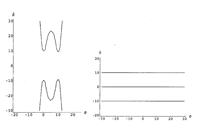
Figure 1: This graph shows the allowed region in the plane $\{\phi(t),\ \dot{\phi}(t)\}$ defined by the Weak Energy Condition. The plot is obtained in the case of $m_{pl}\,=\,10$, $\beta\,=\,10^{-1}m_{pl}$ and $\gamma\,\sim\,m_{pl}$. The left part shows the energy density curve, the regions inside the curve correpond to negative values, which become positive outside. The right panel shows the condition $\rho_{ncbi}+p_{ncbi}\,>\,0$, which are positive between the two straight lines and negative outside. The $\dot{\phi}\,=\,0$ line gives a cosmological constant behavior as implied by the Eq. (31).

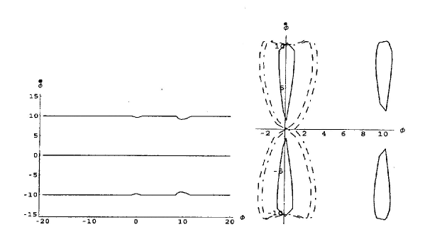
Figure 2: The plot showing the domain in the phase space satisfying the Dominant Energy Condition (left) and the Strong Energy Condition (right). The plot corresponds to the choice of $m_{pl}\,=\,10$, $\beta\,=\,10^{-1}m_{pl}$. The left graphic is not influenced by the choice of different values for the parameter $\gamma$ if $\beta$ is set.h e Strong Energy Condition modifies the contour plots. The three different curves in the right part refer to: $\gamma\,\sim\,m_{pl}$ (solid), $\gamma\,\sim\,10^{-1}m_{pl}$ (dashed) and and $\gamma\,\sim\,10^{-2}m_{pl}$ (dot-dashed). The inner regions correspond to positive energy values while the external ones are negative and provide suitable initial condition for accelerating dynamics.

4.2 Critical points

Let us now investigate the dynamical properties of the NCBI scalar field. In terms of relevant variables only, the system evolves in a four dimensional space ($a(t),\dot{a}(t),\phi,\dot{\phi}(t)$) which can be reduced to a three-dimensional set. In fact, in a spatially flat case it is possible to introduce the Hubble parameter as an independent variable and to study the three-dimensional phase space ($H,\phi,\dot{\phi}$) (here and in the following we neglect the explicit time dependence of dynamical variables). Furthermore, the Friedmann equation provides a surface in this three dimensional space, implying that the relevant dynamics can be followed on this two-dimensional surface.

However, due to the complexity of the model, it is impossible to get an explicit expression of both $H$ and $\dot{\phi}$. To overcome this problem, a reasonable approach is to solve the field equations numerically and to reconstruct the phase space curves for several values of parameters.

The first thing to do while performing a qualitative study is to find the critical points of the system. The critical points of the scalar field can be obtained by solving Eq.(25) with $\dot{\phi}=0\,\,\text{and}\,\,\ddot{\phi}(t)=0$, they are obtained the three values $\phi=0,\ \gamma\sqrt{3}/2\ \text{or}\ \gamma\sqrt{3}$. On the other side, the critical points of the full system are obtained considering also the other field equations. From the cosmological point of view they correspond to de Sitter solutions with constant scalar field. The general situation can be summarized as follows:

$$\left(H,\phi\right)\,=\,\left\{\begin{array}[]{lr}\ (0,0)\ \ \ \ \ \ \ \ \ \ \mbox{Minkowski}\,,\\ \\ \left(\left(\frac{1}{3}\frac{\beta^{2}}{m^{2}_{Pl}}\left(\left(1+\beta^{-2}\gamma^{4}\right)^{\frac{1}{2}}\left(1+\frac{\beta^{-2}\gamma^{4}}{4}\right)^{\frac{1}{4}}\right)-1\right)^{\frac{1}{2}},\frac{\gamma\sqrt{3}}{2}\right)\ \ \mbox{de Sitter}\,,\\ \\ \ \left(0,\gamma\sqrt{3}\right)\ \ \ \ \ \ \ \,\mbox{Minkowski}\,.\end{array}\right.$$ (38)

The first and the third fixed points correspond to trivial Minkowski spaces [32]. In fact from the definition of the energy density (26) and pressure (27) we see that in these cases both do vanish. In other words there is no source for dynamics and the system reduces to a Minkowski space-time.

The second fixed point is a typical de Sitter solution with the equation of state for a scalar field of the cosmological constant type. The energy density is different from zero and provides a source for the exponential expansion:

$$\rho_{ncbi}^{deSitter}={\beta^{2}}\left\{\left(1+\beta^{-2}\gamma^{4}\right)^{1/2}\left(1+\frac{\beta^{-2}\gamma^{4}}{4}\right)^{1/4}-1\right\}.$$ (39)

As we will see later, in our model this solution is no more an attractor in the usual sense. In fact, there are some values of the parameters for which phase trajectories deviate from the de Sitter solution even if the initial conditions are taken very close to this fixed point. This result does not agree with the the No-Hair Theorem [34] which holds for general cosmological models containing scalar field, as demonstrated in [32] both with a minimal and a non-minimal coupling cases. Similar results concerning the dynamics of a Born-Infeld scalar field system have been recently obtained in [33].

The interpretation of the scalar field fixed points becomes obvious with the Born-Infeld relaxed limit analyzed in the previous section. It is easy to check that the two values $\phi(t)=(0,\sqrt{3}\gamma)$ correspond to the true vacuum configuration of the top hat potential in Eq.(29) while $\phi(t)=\sqrt{3}/2\gamma$ corresponds to the unstable “false vacuum" state. In what follows, we shall sometimes refer to these states as with the usual double-well Higgs potential. Let us now analyze the stability of the fixed points. We can rewrite the NCBI lagrangian (19) in a new form and rescale the scalar field by substituting $\phi\rightarrow\sqrt{3}\phi$:

$${\cal{L}}_{ncbi} =\beta\left[1-{\left({\left(1-\frac{3\,{\dot{\phi}}^{2}}{{\beta}^{2}}\right)}^{2}+\frac{16\,{\phi}^{2}\,{\left(-\gamma+\phi\right)}^{2}}{{\beta}^{2}}\right)}^{\frac{1}{4}}\left(1+\frac{4\,{\phi}^{2}\,{\left(-\gamma+\phi\right)}^{2}}{{\beta}^{2}}\right)^{\frac{1}{2}}\right]$$

In the vicinity of singular points we observe behaviors similar to those of a scalar field minimally coupled to gravity [35], with energy density given by:

$$\rho=b(\frac{1}{2}\dot{\phi}^{2}+\frac{1}{2}m^{2}\phi^{2})+\rho_{0}\,.$$ (40)

For each fixed point, the parameters $m^{2}$ and $\rho_{0}$ should be expressed in terms of the parameters $\beta$ and $\gamma$ (the parameter $b$ is not relevant for the stability analysis). We just saw that for the “Born-Infeld scalar field” there are the three fixed points (38), which in terms of the scalar field variables $\phi,\dot{\phi}$ are given by $(\phi=0,\ \dot{\phi}=0)$, $(\phi=\gamma,\ \dot{\phi}=0)$ and $(\phi=\frac{\gamma}{2},\ \dot{\phi}=0)$.

Now, linearizing the equations of motion around these fixed points and evaluating the corresponding Jacobian matrices, we infer the exact character of each singular point [36]. For the two asymptotic Minkowskian solutions, that is at the points $(\phi=0,\ \dot{\phi}=0)$ and $(\phi=\gamma,\ \dot{\phi}=0)$, we find that

$$m^{2}=4\gamma^{2}\ \ \ \ \ \ \ \ \ \rho_{0}=0\,.$$ (41)

which corresponds to a stable point with eigenvalues in the $(\phi,\ \dot{\phi})$ plane: $\lambda_{{\pm}}=\pm i2\gamma$, both complex. In the case of the point $(\phi=\frac{\gamma}{2},\ \dot{\phi}=0)$ we find

$$m^{2}\,=\,-2\gamma^{2}\frac{(1+\displaystyle\frac{\gamma^{4}}{2\beta^{2}})}{(1+\displaystyle\frac{\gamma^{4}}{4\beta^{2}})}\,\ \ \,\ \ \rho_{0}\,=\,\left(1+\frac{\gamma^{4}}{\beta^{2}}\right)^{\frac{1}{4}}\sqrt{1+\frac{\gamma^{4}}{4\beta^{2}}}-\,1\,.$$ (42)

Hence, because $m^{2}$ is negative, it corresponds to an unstable point, and the eigenvalues in the plane $(\phi,u)$ are:

$$\lambda_{+}\,=\,\displaystyle\frac{3H_{0}}{2}(\sqrt{1-\frac{4m^{2}}{9H_{0}^{2}}}-1)>0\,\ \ \,\ \ \lambda_{-}\,=\,-\displaystyle\frac{3H_{0}}{2}(1-\sqrt{1-\frac{4m^{2}}{9H_{0}^{2}}})<0$$ (43)

with $H_{0}=\sqrt{\frac{\kappa^{2}}{3}\rho_{0}}$. In terms of $\beta$ and $\gamma$, the eigenvalues take on the following form:

$$\lambda_{+}\,=\,\frac{3}{2\sqrt{6}}\,{\sqrt{-2+{\left(1+\frac{{\gamma}^{4}}{{\beta}^{2}}\right)}^{\frac{1}{4}}\,{\sqrt{4+\frac{{\gamma}^{4}}{{\beta}^{2}}}}}}\ \times\\ \left(-1+\,{\sqrt{1+\frac{32\,{\gamma}^{2}\,\left(2\,{\beta}^{2}+{\gamma}^{4}\right)}{3\,\left(4\,{\beta}^{2}+{\gamma}^{4}\right)\,\left(-2+{\left(1+\frac{{\gamma}^{4}}{{\beta}^{2}}\right)}^{\frac{1}{4}}\,{\sqrt{4+\frac{{\gamma}^{4}}{{\beta}^{2}}}}\right)}}}\right)$$ (44)

$$\lambda_{-}\,=\,\frac{-3}{2\sqrt{6}}{\sqrt{-2+{\left(1+\frac{{\gamma}^{4}}{{\beta}^{2}}\right)}^{\frac{1}{4}}\,{\sqrt{4+\frac{{\gamma}^{4}}{{\beta}^{2}}}}}}\,\times\\ \left(1+{\sqrt{1+\frac{32\,{\gamma}^{2}\,\left(2\,{\beta}^{2}+{\gamma}^{4}\right)}{3\,\left(4\,{\beta}^{2}+{\gamma}^{4}\right)\,\left(-2+{\left(1+\frac{{\gamma}^{4}}{{\beta}^{2}}\right)}^{\frac{1}{4}}\,{\sqrt{4+\frac{{\gamma}^{4}}{{\beta}^{2}}}}\right)}}}\right)$$ (45)

The most interesting feature for the stability study is the sign of $\lambda_{+}$ and $\lambda_{-}$ which is not easy to determine. However, after the expansion in powers of $\beta$ for $\lambda_{\pm}$ these expressions are considerably simplified:

$$\lambda_{+}\,=\,\displaystyle\sqrt{2}\gamma-\frac{3}{4}\sqrt{\frac{\gamma^{4}}{2\beta^{2}}}+o(\frac{1}{\beta^{2}})\,\ \ \,\\ \,\lambda_{-}\,=\,-\displaystyle\sqrt{2}\gamma-\frac{3}{4}\sqrt{\frac{\gamma^{4}}{2\beta^{2}}}+o(\frac{1}{\beta^{2}})\,.$$ (46)

4.3 Numerical Analysis

Our dynamical system is characterized by three parameters $\beta,\ \gamma,\ m_{Pl}$, which in the case of flat space geometry determine it completely. However it is obvious that only two of them are independent. To perform the numerical analysis we have considered $\beta,\gamma$ in terms of the normalized Planck mass. In order to explore a dimensionally uniform parameter space we consider $1/\beta,1/\gamma^{2},1/m^{2}_{Pl}$ .

The parameters $\beta$ and $\gamma$ cannot take on arbitrary values if we have to satisfy the following physical requirements:

• the characteristic Born-Infeld parameter cannot be higher than the squared Planck length, i.e. $\beta\lesssim{m^{2}_{Pl}}$;

• the mass parameter also can not be greater than the Planck mass, i.e. $\gamma^{2}\lesssim{m^{2}_{Pl}}$.

Taking into account these constraints we have explored the space of the parameters considering a domain ranging from fractions of the Planck constant to its entire value. To perform a numerical analysis we have fixed the value of $m_{Pl}$ at 10, so that the essential features of the phase space behavior can be clearly displayed. To give a picture of the results we have considered $\beta\in[10^{-2}m^{2}_{Pl}\,,m^{2}_{Pl}]$ (namely with $m_{Pl}=10$, $1/\beta\in[10^{-2},1]$) and $\gamma\in[10^{-2}m_{Pl}\,,m_{Pl}]$ ($1/\gamma^{2}\in[10^{-2},100]$).

The definition of the lagrangian and the field equations impose some natural constraints in the phase space $\{\phi\ ,\dot{\phi}\}$. The lagrangian (19) contains an even root term, this means that the term under the root must be positive. Indeed it is as it is a sum of two squared terms. Let us look at the field equations. The Friedmannn equation (23), in the spatially flat case we are considering, implies the positivity of energy density $\rho_{ncbi}\geq{0}$. This gives the first constraint on the phase space of the scalar field as we already saw in Fig.1. Let us also note that there are no divergences in the definition of the energy density and that it remains always finite.

Considering now the pressure equation (24) we observe that the only constraint is again the positivity of the function under root, but it leads to the same constraints as those imposed by the lagrangian itself.

The analysis of the scalar field equation (25) is more complex. Here we observe that if the function multiplying the $\ddot{\phi}(t)$ term is zero than the term $\ddot{\phi}(t)$ can become divergent. This implies, as in the case without gravity [6], that there exists a characteristic curve in the phase space where the solutions for the scalar field become divergent in a finite time. This problem can be cured if all other terms in the equation simultaneously vanish. This allows $\ddot{\phi}(t)$ to remain finite and provides some crossing points in the phase space on the separatrix were the system can go beyond this curve. The singular curve ’separatrix) is given by the following relation:

$$\left(1+\frac{4}{9}\Pi^{2}[\phi(t)]\right)\left\{\left(1-\beta^{-2}\dot{\phi}^{2}(t)\right)^{2}+\frac{16}{9}\Pi^{2}[\phi(t)]\left(1-3\beta^{-2}\dot{\phi}^{2}(t)\right)\right\}=0\,.$$ (47)

Now, comparing with the pure Higgs field case studied in [6] there is an obvious and important difference. The presence of gravity, which induces the new constraint $\rho_{ncbi}\geq 0$ implies the absence of crossing points over the divergence curve.

With the allowed regions thus defined, the following step is to plot the characteristic curves generated by the scalar field equation. The cosmological evolution of the model and the scale factor behavior are driven by the scalar field dynamics.

At this point we are ready to perform a numerical study of the system. In the following we will present the results for three combinations of parameters expressed in terms of the Planck mass:

Case: $\beta=m^{2}_{Pl}$.
The system displays similar phase trajectories for all values of mass parameter (we plot the case $\gamma\sim m_{Pl}$ and $\gamma\sim 10^{-1}m_{Pl}$). The scalar field shows a spiralling behavior ending up in one of the two stable fixed points.

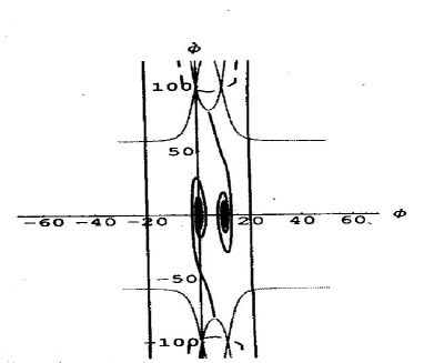
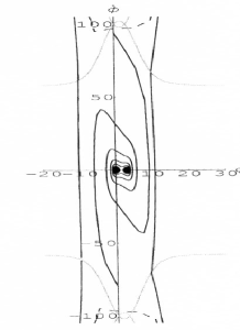
Figure 3: Phase space of the scalar field in the case $\beta=m^{2}_{Pl}$ with $\gamma\sim m_{Pl}$ and $\gamma\sim 10^{-1}m_{Pl}$. The dashed curve is the constraint obtained by the Weak Energy Condition (as yet seen in Fig.1), while the lighter one is the characteristic curve due to the scalar field equation. We show only some characteristic curves since for other initial conditions the shape is analogous.

The time evolution on phase trajectories is from left to right. For smaller values of $\gamma$ the allowed region around the fixed points becomes narrower. This is understandable because the mass parameter in the standard $\phi^{4}(t)$ theory controls the width of the potential. One obvious difference with the case analyzed in [6] is the spiraling behavior. This effect is due to the presence of a friction term in the scalar field equation coming from the gravitational interaction. The pure Born-Infeld regime is recovered when one increases the values of the Planck mass (equivalent with a decrease of gravitational coupling) and fixes the other parameters. On the other side if one increases the $\beta$ parameter the effect is to widen the allowed domain along the $\dot{\phi}(t)$ direction. This transforms the system into the standard Higgs case in presence of gravity obtained in the relaxed limit (18).

A particular result visible in Fig.(3) is that the physically significant dynamics is constrained to a very small region around the fixed points. All the trajectories with different initial conditions intersect the singular curve in a finite time. This entails a singular behavior for the scale factor thus excluding such solutions. It is easy to find the cases in which it is possible to get inflationary behavior. In general (see Tab.2) non-linearities combined with a small enough mass parameter make the scalar field roll down too quickly, never attaining a slow rolling regime. This implies that the scale factor follows a power law regime since the beginning.

This conclusion results from examining the slow rolling parameter $\varepsilon=-\frac{\dot{H}(t)}{H^{2}(t)}$ [29]. It is well known that this parameter should be significatively smaller than 1 throughout all the inflationary expansion.
In the cases $\gamma\sim\,m_{Pl}$, $\gamma\sim\,10^{-1}m_{Pl}$ and $\gamma\sim\,10^{-1}m_{Pl}$ with a slow rolling-type initial condition from the top of the unstable fixed point, it is possible to get inflationary evolution with the right power law phase transition at a given stage.
Case: $\beta=m^{2}_{Pl}/10$.
We examine the plot with $\gamma$ of the same order of the Planck mass. This plot is quite interesting since it is clear that the two stable fixed points define two separate regions between which there are no trajectories. The other cases with smaller values of the mass parameter recall quite similar shapes to the previous case.

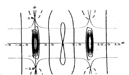
Figure 4: Phase space of the scalar field in the case $\beta=,m^{2}_{Pl}/10$ with $\gamma\sim\,m_{Pl}$. The dashed curve is the constraint imposed by the Friedmann equation, while the thinner one is due to the scalar field equation. We limit the number of solutions plotted to make the results clearly visible.

Around the two fixed points there are stable spiralling solutions. The trajectories starting from the unstable fixed point hit the singular curve in a finite time. They describe closed lines broken by the characteristic curve. If the initial velocity is small enough, the scalar field remains in the unstable critical point for a long time and then it joins again the characteristic curve in finite time since the remaining part of the phase space is forbidden. This provides an infinite inflationary solution of cosmological constant type. It is obvious that in this case the de Sitter solution is no more an attractor. The initial conditions taken close enough to the unstable fixed point instead of providing inflationary de Sitter like solutions give power law trajectories which never collapse into the stable vacuum state intersecting the $\ddot{\phi}=\infty$ curve instead.

In other cases the behavior is similar to the previous case with $\beta=m^{2}_{Pl}$. Again no inflation is observed, and the slow rolling parameter $\varepsilon$ is always greater than one. On the other side the phase space obtained with $\gamma=10^{-1}m_{Pl}$ provides the physical condition ensuring inflation and it remains similar to the one shown in Fig.(3). All possible cosmological behaviors of the model are given in Tab.(2), also for the values of parameters not considered in the plots.

$m_{Pl}=10$	$\beta\rightarrow{10m^{2}_{Pl}}$	$m^{2}_{Pl}$	$10^{-1}m^{2}_{Pl}$	$10^{-2}m^{2}_{Pl}$	$10^{-3}m^{2}_{Pl}$	$10^{-4}m^{2}_{Pl}$	$10^{-5}m^{2}_{Pl}$
$\gamma\rightarrow{m_{Pl}}/\sqrt{3}$	$-$	$+$	$+$	$+$	$+$	$-$	$-$
$m_{Pl}10^{-1}/\sqrt{3}$	$-$	$+$	$+$	$+$	$+$	$+$	$-$
$m_{Pl}10^{-2}/\sqrt{3}$	$-$	$+$	$-$	$-$	$-$	$-$	$-$
$m_{Pl}10^{-3}/\sqrt{3}$	$-$	$-$	$-$	$-$	$-$	$-$	$-$
$m_{Pl}10^{-4}/\sqrt{3}$	$-$	$-$	$-$	$-$	$-$	$-$	$-$
$m_{Pl}10^{-5}/\sqrt{3}$	$-$	$-$	$-$	$-$	$-$	$-$	$-$
$m_{Pl}10^{-6}/\sqrt{3}$	$-$	$-$	$-$	$-$	$-$	$-$	$-$

Table 2: A summary of the capability of providing inflation for the NCBI cosmological model. The combination of parameters allowing inflation are indicated with a sign $+$, the wrong ones whit a $-$. It is obvious that this model can provide inflation only if the mass of the scalar field is close the Planck mass. With small values of $\beta$ we get the strong BI regime, it appears that in this case only some particular configuration of parameters allow inflation.

We have tested also the amount of inflation provided by the NCBI model. Via numerical evaluation of $\phi(t)$ it was possible to calculate the winding number of trajectoriy by means of the relation

$$N\equiv\,\ln\frac{a(t_{end})}{a(t_{initial})}=\int_{t_{i}}^{t_{e}}H\,dt\,.$$ (48)

We see that the NCBI scalar model can generate the right amount of inflation (more than 60), if proper slow rolling conditions are imposed. The expansion rate of this model is lower than the one obtained with the corresponding Born-Infeld relaxed lagrangian (29).

Case: $\beta=10^{-2}m^{2}_{Pl}$.
This case represents the strong Born-Infeld limit in relation to the small value of the Born-Infeld parameter. The shape of the phase space is similar to the ones proposed before, with the big feature that the allowed region is strongly constrained. From the cosmological point of view the behavior is quite the same of the case with $\beta=10^{-1}m^{2}_{Pl}$. In relation to the variation of $\gamma$ is possible to obtain inflation only for some condition of the mass parameter. In Fig.5 we show two cases, again the solution $\gamma=10^{-1}m_{Pl}$ shows a particular behavior as in precedence, the following cosmological properties are similar to the previous case. Another interesting phenomena appears even in the second plot when the mass-shell of the scalar field is close to the Planck scale. In such a case the wrapping of the phase lines evolves moving around both the two static fixed points while the stationary configuration is achieved ending in one of this points in relation to the initial condition without any particular rule, see Fig.6. This happens for initial conditions which are chosen for all the three fixed points with several values of the velocity $\dot{\phi}$.
Interesting plots are shown in Fig.7. In this case a configuration of the parameters is chosen in such a way that the gravitational coupling happens to be relaxed while the BI coupling is strong. The net effect is that the spiralling behavior around stable fixed points in the left plot of Fig.5 is more similar to the one proposed in [6]. Closed trajectories shown in absence of gravity are no more possible due to the friction term and are transformed into spirals. No significant differences are found with the variation of the mass parameter.

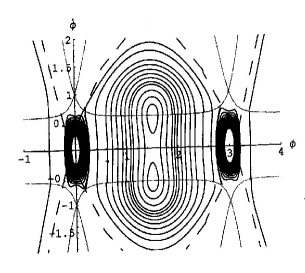
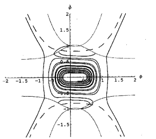
Figure 5: Phase space of the scalar field in the case $\beta=m^{2}_{Pl}/100$ with $\gamma=10^{-1}m_{Pl}$ and $\gamma=10^{-2}m_{Pl}$. In the second plot the region in the middle of the curve trajectories (small values of $\dot{\phi}$, left in white) has been plotted in detail in figure 6. It is obvious a behavior similar to the one found in [6] affected by the spiraling shape of the trajectories due to the gravitational interaction.

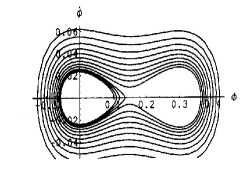
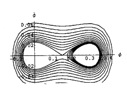
Figure 6: The detail of the previous plot, it is showed how the wrapping of the solutions in proximity of the critical points changes in relation to the initial conditions, left side $\phi\,=\,0,\ \dot{\phi}\,=\,0.16$ and right $\phi\,=\,0,\ \dot{\phi}\,=\,0.18$. This behavior is alternated, for $\dot{\phi}\,=\,0.36$ the solutions converges to $\phi\,=\,0$ while for $\phi\,=\,0.6$ again versus $\phi\,=\,0.33$.

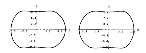
Figure 7: The phase portrait in the case of low gravitational coupling. A strong similarity is found with the results of [6]. The gravitational interactions break the steady state configuration of solutions; the thickness of the line is due to the very slow spiralling of the trajectory.

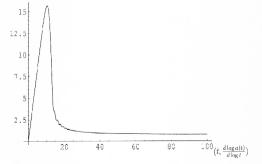
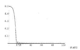
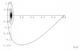
Figure 8: The simultaneous evolution of the Hubble parameter and of the scalar BI field. The last graph is the phase space plot of $\phi,\dot{\phi}$; the trajectory is spiralling towards the singular point.

The simultaneous evolution of the cosmological scale factor $a(t)$ (through its logarithmic derivative with respect to $\ln t$) and of the scalar field $\phi$ is displayed in Fig. 8:

5 Discussion and conclusions

In this paper we propose the cosmological analysis of a NCBI model obtained from the matrix realization of a non-commutative geometry. This study represents the gravity coupled generalization of a model proposed in [6]. To determine the cosmological properties of the model and its physical relevance in this sense we have investigated numerically the NCBI scalar field dynamics constructing its phase space characteristic curves. The cosmological results, in relation to several values of the parameters, are summarized in Tab.(2).

It is possible to observe that there are different behaviors, but in any case inflation can be recovered when the mass of the scalar field is close to the Planck mass. A relevant difference with the $\phi^{4}(t)$ limit, is that the obtained amount of inflation is smaller, although enough to solve the several shortcomings of the standard cosmological models.

The scalar field shows a phase space which is similar to the standard case, without a BI cut-off, if $\beta$ is big in comparison to the other parameters. In the other cases the dynamics develops inside a constrained region around the critical points. However, the bounded regions distinctive of the Born-Infeld free theory [6] are lost because of the presence of the cosmological friction term. A shape similar to the pure BI case can be observed in Fig. 7, but it is obvious a slow spiralling rate of the trajectories as a slowly decaying in the stable vacuum minima.

The most important difference with the standard case is that in the BI realm all the dynamics is always constrained inside a well defined region. This is a persisting feature which can be found in all phase space plots. Since for a strong BI coupling the physically significant region is very reduced both in the velocity and in the scalar field values, this means that such a framework possesses an intrinsic condition that the scalar field should move starting only near the critical points. This is more obvious when the Born-Infeld parameter is small. All other initial conditions will provide trajectories which will intersect the singular line in a finite time leading to physically meaningless solutions. In some sense this approach contains in itself a particular choice of initial conditions without any fine tuning procedure.

In order to decide whether the scalar NCBI model is a viable approach of inflation, still a large amount of work is needed, above all with respect to the observational predictions of the model. It should be interesting to verify whether such a model can represent a good candidate for the quintessential inflation [37]. It is interesting to ask if the high non-linearity of the NCBI approach can preserve safe contributes even in the late time epoch able to generate a driving force for the new accelerating phase of cosmic expansion. These questions remain beyond the scope of the present paper.

Acknowledgment A. T. is very grateful for the hospitality at the Laboratoires de Physique Theorique des Liquides of the University Paris VI Pierre et Marie Curie where this work has been substantially developed.

References

- [1] Mie G., Annalen der Physik 37 (1912) 551.
- [2] Born M., Infeld L., Proc. Roy. Soc. Lond. A 144 425-451 (1934).
- [3] Hagiwara T., J. Phys. A 14 3059 (1981)
- [4] Tseytlin A.A., Nucl. Phys. B 501, 41-52 (1997).
- [5] Park J.H., Phys. Lett. B 458, 471-476, (1999).
- [6] Sérié E., Masson T., Kerner R., Phys. Rev. D, (2004).
- [7] Sérié E., Masson T., Kerner R., Phys. Rev. D 68, 125003, (2003).
- [8] Sérié E., PhD thesis, Université Paris 6, 2005.
- [9] Garcia-Salcedo R., Breton N., Int. Journ. Mod. Phys. A 15, 27, 4341 (2000).
- [10] Galtsov et al., Phys. Rev. D 65, 084007 (2002).
- [11] Meng X. H., Wang P., Class. Quant. Grav. 21, L101 (2004).
- [12] Elizalde E., Lindsey J.E., Nojiri S., Odintsov S., Phys.Lett. B 574, 1 (2003).
- [13] Tseytlin A.A., contribution to Yuri Golfand memorial volume, arXiv:preprint hep-th/9908105.
- [14] Kerner R., Barbosa A.L., Galtsov D.V., Proceedings of XXXVII Karpacz Winter School edited in the Proceedings Series of American Mathematical Society, editors J. Lukierski and J. Rembielinski, arXiv: preprint hep-th/0108026.
- [15] Dubois-Violette M., Kerner R., Madore J., J. Math. Phys. 31, 323, (1990).
- [16] Dubois-Violette M., Kerner R., Madore J., J. Math. Phys. 31, 331, (1990).
- [17] Dubois-Violette M., Kerner R., Madore J., Phys.Lett. B B217 , 485 (1989)
- [18] Peebles P.J.E., Rev.Mod.Phys. 75, 559 (2003).
- [19] Bento M.C., Bertolami O., Sen A.A., Phys. Rev. D 66, 043507 (2002); Bento M.C., Bertolami O., Sen A.A., Phys. Rev. D 67, 063003 (2003).
- [20] Shani V., Proceedings of the Second Aegean Summer School on the Early Universe, Syros, Greece (2003), arXiv:astro-ph/0403324.
- [21] N. Bilic, G. B. Tupper and R. D. Viollier, Phys. Lett. B 535, 17 (2002), astro-ph/0111325.
- [22] Guth A., Phys. Rev. D 23, 347 (1981); Phys.Lett.B 108, 389 (1982).
- [23] de Vega H.J., “Early cosmology and fundamental physics,” pre-print arXiv:astro-ph/0307477; Cao F.J., de Vega H.J., Sanchez N.G., arXiv:astro-ph/0406168.
- [24] Smoot G.F., et al., Astrophys. J. 396, L1 (1992).
- [25] de Bernardis P., et al., (BOOMERaNG collaboration), Nature 404, 955 (2000); Balbi A., et al., (MAXIMA Collaboration), Astrophys. J. 558, L145-L146 (2001);
- [26] Spergel D.N., et al., Astrophys. J. Suppl. 148, 175 (2003); C.L. Bennett et al., Astrophys. J. Suppl. 148, 1 (2003).
- [27] Liddle A., proceedings of ICTP summer school in high-energy physics, 1998, arXiv: astro-ph/9901124.
- [28] Linde A., Phys. Lett. B 129, 177, (1983).
- [29] Riotto A., Lectures for the "ICTP Summer School on Astroparticle Physics and Cosmology", Trieste, (2002) arXIv: preprint hep-ph/0210162.
- [30] Starobinsky A.A., Phys.Lett. B91, 99 (1980).
- [31] de Ritis R., C. Rubano C., Scudellaro P., Nuovo Cim. B 108, 1243 (1993). (2003); Verde L. et al., ApJS, 148, 195 (2003).
- [32] Gunzig, Faraoni et al. Class. Quantum Grav. 17, 1783-1814, (2000).
- [33] Novello M., Makler M., Werneck L.S., Romero C.A., arXiv: astro-ph/0501643.
- [34] Kolb E.W., Turner M.S., The Early Universe, Addison Wesley Publishing Company, Redwood City (1988).
- [35] Belinski V.A., Khalatnikov I.M., Grishchuk L.P., Zeldovich Y.B., Phys. Lett. B 155, 232 (1985).
- [36] Wainwright J., Ellis G.F.R., Dynamical System in Cosmology, Cambridge Univ. Press, Cambridge, (1997).
- [37] Dimopoulos K., Valle J.W.F., Astropart. Phys. 18, 287 (2002).