Thick Domain Walls in AdS Black Hole Spacetimes

Abstract

Equations of motion for a real self-gravitating scalar field in the background of a black hole with negative cosmological constant were solved numerically. We obtain a sequence of static axisymmetric solutions representing thick domain wall cosmological black hole systems, depending on the mass of black hole, cosmological parameter and the parameter binding black hole mass with the width of the domain wall. For the case of extremal cosmological black hole the expulsion of scalar field from the black hole strongly depends on it.

I Introduction

The early Universe and the phase transitions there provide signs of the high-energy phenomena which are beyond the range of contemporary accelerators  Vilenkin and Shellard (1994). Such topological defects as cosmic strings attracted a great interests and were widely studied in literature. Black hole cosmic string configurations studies revealed the evidences that cosmic string could thread it or could be expelled from black hole. In the case of extreme Reissner-Nordström (RN) black holes it was found that there was a range of the black hole parameters for which the expulsion of the vortex took place Dowker et al. (1992); Achúcarro et al. (1995); Chamblin et al. (1998a, b); Bonjour and Gregory (1998); Bonjour et al. (1999). In dilaton gravity theory being the low-energy limit of the string theory it was also justified Moderski and Rogatko (1998a, b, 1999); Santos and Gregory (2000) that a vortex could be treated by the remote observer as a hair on the black hole. Moreover, extreme dilaton black hole always expel the Higgs field, one has to do with the so-called Meissner effect. The problem of vortices in de Sitter background was analyzed in Ref. Ghezelbash and Mann (2002a), while the behaviour of Abelian Higgs vortex solutions in Schwarzschild anti de Sitter (AdS), Kerr, Kerr-AdS and Reissner-Nordström AdS (RN-AdS) was studied in Refs. Dehghani et al. (2002); Ghezelbash and Mann (2002b). The vortex solution for Abelian Higgs field equations in the background of four-dimensional black string was considered in Ref. Dehghani and Jalali (2002).

The idea that the Universe is embedded in higher-dimensional spacetime acquires much attention. The resurgence is motivated by the possibility of resolving the hierarchy problem Randall and Sundrum (1999a, b), i.e., the difference in magnitudes of the Planck scale and the electroweak scales. Also the most promising candidate for a unified theory of Nature, superstring theory predicts the existence of the so-called D-branes which renew in turn the idea of brane worlds. From this theory point of view the model of brane world stems from the idea presented by Horava and Witten Hořava and Witten (1996a, b). Namely, the strong coupling limit of $E_{8}\times E_{8}$ heterotic string theory at low energy is described by eleven-dimensional supergravity with eleventh dimension compactified on an orbifold with $Z_{2}$ symmetry. The two boundaries of spacetime are ten-dimensional planes, to which gauge theories are confined. Next Witten (1996); Lukas et al. (1999a, b) it was argued that six of the eleven dimensions could be consistently compactified and in the limit spacetime looked five-dimensional with four-dimensional boundary brane.

The studies of the interplay between black holes and domain walls (branes) acquire more attention. The problem of stability of a Nambu-Goto membrane in RN-dS spacetime was studied in Higaki et al. (2001). The gravitationally interacting system of a thick domain wall and Schwarschild black hole was considered in Morisawa et al. (2000, 2003). Emparan et al. Emparan et al. (2001) elaborated the problem of a black hole on a topological domain wall.

In Rogatko (2001) the dilaton black hole-domain wall system was studied analytically and it was revealed that for the extremal dilaton black hole one had to do with the expulsion of the scalar field from the black hole (the so-called Meissner effect). The numerical studies of domain wall in the spacetime of dilaton black hole was considered in Ref. Moderski and Rogatko (2003), where the thickness of the domain wall and a potential of the scalar field $\varphi^{4}$ and sine-Gordon were taken into account. In the case of a real self-interacting scalar field in the background of RN solution it was found that in the extremal case there was a parameter depending on black hole mass and the width of the domain wall which constituted the upper limit for the expulsion to occur Moderski and Rogatko (2004). Dynamics of domain walls intersecting black holes, taking into account the evolution of the system during the separation was elaborated in Flachi et al. (2006).

The importance of introducing the cosmological into considerations comes not only from the theoretical point of view but also for the observational results of our Universe. Small cosmological constant may be an alternative to the dark energy in explanation the observed a type Ia suprenova acceleration. On the other hand, as far as a negative cosmological constant is concerned a tremendous interest has focused on issues related to the AdS spacetime. One of them is the AdS/CFT (conformal field theory) correspondence which states that conformal field theories in d-dimension $R_{d}$ are described in terms of supergravity or string theory on the product spacetime consisting with asymptotically $AdS_{d+1}$ and compact manifold, providing that there are relations between data on the boundary $R_{d}$ of the $AdS_{d+1}$ and the data in the bulk $AdS_{d+1}$ Maldacena (1998); Witten (1998a, b).

Our paper will be devoted to the behaviour of the AdS black hole thick domain wall system. A domain wall will be simulated by a self-interacting scalar field. We shall numerically analyze the behaviour of scalar fields for various value of cosmological parameter. The brief outline of our paper is the following. The next section is devoted to the basic equations of the considered problem. In Sec. III-IV we presented the boundary conditions of the problem as well as the numerical analysis of the equations of motion for the two cases of potentials with discrete sets of minima. Namely, we shall analyze the $\varphi^{4}$ and sine-Gordon potentials. The conclusions and discussions will be presented in Sec. V.

II The basic equations of the problem

In our paper we shall consider a spherically symmetric static black hole with negative cosmological constant. The metric of which is written as follows:

$$ds^{2}=-\left(1-{2M\over r}+{Q\over r^{2}}-{\Lambda\over 3}r^{2}\right)dt^{2}+{dr^{2}\over{\left(1-{2M\over r}+{Q\over r^{2}}-{\Lambda\over 3}r^{2}\right)}}+r^{2}(d\theta^{2}+\sin^{2}\theta d\varphi^{2}),$$ (1)

where we define $\Lambda={-3\over l^{2}}$ and $Q$ is the charge of the considered black hole. In what follows we shall denote by $V(r)=1-{2M\over r}+{Q\over r^{2}}-{\Lambda\over 3}r^{2}$. The condition $V(r)=0$ is a quadratic algebraic equation for $r$. As was mentioned in Romans (1992) the standard closed-form for the above mentioned four roots is rather lengthy and not especially illuminating. In what follows the AdS black hole spacetime will be the background metric on which one solves the domain wall Eqs. of motion. The domain wall will be simulated by a self-interacting scalar field.

A general matter Lagrangian with real Higgs field and the symmetry breaking potential of the form will be taken into account

$${\cal L}_{dw}=-{1\over 2}\nabla_{\mu}\varphi\nabla^{\mu}\varphi-U(\varphi),$$ (2)

where by $\varphi$ we have denoted the real Higgs field, while by $U(\varphi)$ the symmetry breaking potential having a discrete set of degenerate minima. The energy-momentum tensor for the domain wall yields

$$T_{ij}(\varphi)=-{1\over 2}g_{ij}\nabla_{m}\varphi\nabla^{m}\varphi-U(\varphi)g_{ij}+\nabla_{i}\varphi\nabla_{j}\varphi.$$ (3)

For the convenience we scale out parameters via transformation $X={\varphi/\eta}$ and $\epsilon=8\pi G\eta^{2}$. The parameter $\epsilon$ represents the gravitational strength and is connected with the gravitational interaction of the Higgs field. Defining $V(X)={U(\varphi)\over V_{F}}$, where $V_{F}=\lambda\eta^{4}$ we arrive at the following expression:

$$8\pi G{\cal L}_{dw}=-{\epsilon\over w^{2}}\bigg{[}w^{2}{\nabla_{\mu}X\nabla^{\mu}X\over 2}+V(X)\bigg{]},$$ (4)

where $w=\sqrt{{\epsilon\over 8\pi GV_{F}}}$ represents the inverse mass of the scalar after symmetry breaking, which also characterize the width of the wall defect within the theory under consideration. Having in mind (4) the equations for $X$ field may be written as follows:

$$\nabla_{\mu}\nabla^{\mu}X-{1\over w^{2}}{\partial V\over\partial X}=0.$$ (5)

In our considerations we take into account for two cases of potentials with a discrete set of degenerate minima, namely

the $\varphi^{4}$ potential described by the following equation:

$$U_{1}(\varphi)={\lambda\over 4}(\varphi^{2}-\eta^{2})^{2},$$ (6)

and the sine-Gordon potential of the form

$$U_{2}(\varphi)=\lambda\eta^{4}\left[1+\cos(\varphi/\eta)\right].$$ (7)

III The boundary conditions

In the background of the black hole spacetime the equation of motion for the scalar field $X$ implies

$${1\over r^{2}}\partial_{r}\bigg{[}\big{(}r^{2}-2Mr+Q^{2}-{\Lambda\over 3}r^{4}\big{)}\partial_{r}X\bigg{]}+{1\over r^{2}\sin\theta}\partial_{\theta}\bigg{[}\sin\theta\partial_{\theta}X\bigg{]}={1\over w^{2}}{\partial V\over\partial X}.$$ (8)

Consequently, having in mind relation (3) one can define the following quantity for the scalar field $\varphi$:

$$\tilde{E}={T_{t}{}{}^{t}\over{\lambda}\eta^{4}}=\bigg{[}-{1\over 2}\big{(}X_{,r}\big{)}^{2}\bigg{(}1-{2M\over r}+{Q\over r^{2}}-{\Lambda\over 3}r^{2}\bigg{)}-{1\over 2}\big{(}X_{,\theta}\big{)}^{2}{1\over r^{2}}\bigg{]}{w^{2}}-V(X).$$ (9)

As we have to do with non-asymptotically flat spacetime it cannot be interpreted as an energy density of scalar field. On the horizon of the black hole one has the following boundary conditions:

$$V^{\prime}(r_{BH})\partial_{r}X\mid_{r=r_{BH}}=-{1\over r_{BH}^{2}\sin\theta}\partial_{\theta}\bigg{[}\sin\theta\partial_{\theta}X\bigg{]}+{1\over w^{2}}{\partial V\over\partial X}.$$ (10)

As in Refs. Moderski and Rogatko (2003, 2004) we shall restrict our investigations to the case when the core of the domain wall is located in the equatorial plane, i.e., $\theta=\pi/2$. One ought also to impose the Dirichlet boundary conditions at the equatorial plane as follows:

$$X\mid_{\theta={\pi\over 2}}=0,$$ (11)

and the regularity condition for scalar field on the symmetry axis requiring the Neumann boundary condition on $z$-axis in the form as

$${\partial X\over\partial\theta}\mid_{\theta=0}=0.$$ (12)

In order to find the solution of the problem our first task will be to establish the asymptotically behaviour of the scalar field at the large distances. Further it will be necessary to find the numerical solution of its equation of motion.

In this case at large distances from the horizon we demand that the black hole domain wall solution ought to be solution of the domain wall in AdS or dS spacetime. Defining the metric as follows:

$$ds^{2}=-\bigg{(}1+{kr^{2}\over l^{2}}\bigg{)}dt^{2}+{dr^{2}\over\bigg{(}1+{kr^{2}\over l^{2}}\bigg{)}}+r^{2}(d\theta^{2}+\sin^{2}\theta d\varphi^{2}),$$ (13)

where $k=-1$ we have for AdS spacetime, on the other hand $k=1$ is responsible for dS one, the equation of motion for the scalar field $X$ yields

$$\bigg{(}1+{kr^{2}\over l^{2}}\bigg{)}\partial_{r}^{2}X+{2\over r}\bigg{(}1+{2kr^{2}\over l^{2}}\bigg{)}\partial_{r}X+{1\over r^{2}}\partial_{\theta}^{2}X+{1\over r^{2}}\cot\theta~{}\partial_{\theta}X-{1\over w^{2}}{\partial V\over\partial X}=0.$$ (14)

As in Ref. Ghezelbash and Mann (2002a) we set $\rho=r\cos\theta$ and the scalar field $X$ is a function of $\rho$. By virtue of this equations of motion may be written in the form as

$$\bigg{(}1+{k\rho^{2}\over l^{2}}\bigg{)}X_{,\rho\rho}+{4k\rho\over l^{2}}X_{,\rho}-{1\over w^{2}}{\partial V\over\partial X}=0.$$ (15)

Let us solve the equation for the potential $V(X)={1\over 4}(X^{2}-1)^{2}$. The analitycal solution of Eq. (15) is not known, but we shall search for the solution for magnitude of scalar field $X(\rho)$ at constant large distances, i.e., for $\rho\rightarrow\infty$. It follows in particular that $X(\rho\rightarrow\infty)=1=X_{0}$. Equation (15) is approximately satisfied by $X_{0}\simeq 1$, where $X_{0}$ is the minimum of the potential. Denoting fluctuations about this minimum by $\psi(\rho)$ we have the following:

$$X(\rho)=X_{0}+\psi(\rho).$$ (16)

It can be verified by expanding the scalar field $X$ in the equation of motion that it reduces to the form

$$k\rho^{2}\psi_{,\rho\rho}+4k\rho\psi_{,\rho}+{l^{2}\over w^{2}}\psi=0.$$ (17)

In deriving Eq. (17) one has neglected terms of order of unity in coefficients in first and second terms with respect to the terms involving derivatives of scalar field connected with ${\rho^{2}\over l^{2}}$.

Thus, Eq. (17) for large $\rho\rightarrow\infty$ has the approximate solution in the form of

$$X(\rho)\simeq X_{0}\bigg{[}1-\bigg{(}{\rho\over\rho_{0}}\bigg{)}^{{-3+\sqrt{9-4\beta}\over 2}}\bigg{]},$$ (18)

where $\beta={l^{2}/w^{2}k}$, in our case $\beta<0$. The same procedure applied to the sine-Gordon potential $V(X)=1+\cos X$ case reveals the following relation:

$$X(\rho)\simeq X_{0}\bigg{[}1-\bigg{(}{\rho\over\rho_{0}}\bigg{)}^{-2+\sqrt{4-\beta}}\bigg{]}.$$ (19)

IV Numerical calculations

IV.1 Cosmological AdS black hole – $\phi^{4}$ potential

Having laid out for our considerations, we proceed to describe the numerical analysis of the problem. First, we convert to equation of motion (8) to the form more suitable for finite differencing, namely one has the following:

$$\partial_{r}\left[\left(r^{2}-2Mr+Q^{2}+\frac{1}{l^{2}}r^{4}\right)\partial_{r}X\right]\frac{1}{\sin\theta}\partial_{\theta}\left(\sin\theta\partial_{\theta}X\right)-\frac{r^{2}}{w^{2}}X\left(X^{2}-1\right)=0,$$ (20)

or making the differentiation with respect to $r$ coordinate lead us to

$$\left(r^{2}-2Mr+Q^{2}+\frac{1}{l^{2}}r^{4}\right)\partial_{rr}X+2\left(r-M+\frac{2}{l^{2}}r^{3}\right)\partial_{r}X$$ (21)

$$+\partial_{\theta\theta}X+\frac{1}{\tan\theta}\partial_{\theta}X-\frac{r^{2}}{w^{2}}X\left(X^{2}-1\right)=0.$$

Next, we define the quantities

$$a\equiv r^{2}-2Mr+Q^{2}+\frac{1}{l^{2}}r^{4},~{}~{}~{}~{}~{}~{}~{}b\equiv r-M+\frac{2}{l^{2}}r^{3}.$$ (22)

It enables us to rewrite Eq. (IV.1) in the form as follows:

$$a\partial_{rr}X+2b\partial_{r}X+\partial_{\theta\theta}X+\frac{1}{\tan\theta}\partial_{\theta}X-\frac{r^{2}}{w^{2}}X\left(X^{2}-1\right)=0.$$ (23)

Using the notation from our previous work Moderski and Rogatko (2003) Eq. (23) can be rewritten in the finite differences form. It implies

$$a\frac{X_{+0}-2X_{00}+X_{-0}}{(\Delta r)^{2}}+2b\frac{X_{+0}-X_{-0}}{2\Delta r}$$ (24)

$$+\frac{X_{0+}-2X_{00}+X_{0-}}{(\Delta\theta)^{2}}+\frac{1}{\tan\theta}\frac{X_{0+}-X_{0-}}{2\Delta\theta}-\frac{r^{2}}{w^{2}}X_{00}\left(X_{00}^{2}-1\right)=0,$$

or it can be rewritten in a more suitable form for our considerations. Consequently, Eq. (IV.1) yields the result that:

$$\left[\frac{a}{(\Delta r)^{2}}+\frac{b}{\Delta r}\right]X_{+0}+\left[\frac{a}{(\Delta r)^{2}}-\frac{b}{\Delta r}\right]X_{-0}+\left[\frac{1}{(\Delta\theta)^{2}}+\frac{1}{2\Delta\theta\tan\theta}\right]X_{0+}$$ (25)

$$+\left[\frac{1}{(\Delta\theta)^{2}}-\frac{1}{2\Delta\theta\tan\theta}\right]X_{0-}+\left[-\frac{2a}{(\Delta r)^{2}}-\frac{2}{(\Delta\theta)^{2}}-\frac{r^{2}}{w^{2}}(X_{00}^{2}-1)\right]X_{00}=0.$$

We solve the equation (IV.1) using simultaneously over-relaxation (SOR) method Press et al. (1992). A general form of the second-order elliptic equation, finite differenced, yields

$$Ax_{+0}+Bx_{-0}+Cx_{0+}+Dx_{0-}+Ex_{00}=F.$$ (26)

Equation (IV.1) can be brought to the form of relation (26) with the following coefficients for the SOR method for our problem:

$$A=\frac{a}{(\Delta r)^{2}}+\frac{b}{\Delta r},$$ (27)

$$B=\frac{a}{(\Delta r)^{2}}-\frac{b}{\Delta r},$$ (28)

$$C=\frac{1}{(\Delta\theta)^{2}}+\frac{1}{2\Delta\theta\tan\theta_{k}},$$ (29)

$$D=\frac{1}{(\Delta\theta)^{2}}-\frac{1}{2\Delta\theta\tan\theta_{k}},$$ (30)

$$E=-\frac{2}{(\Delta r)^{2}}-\frac{2}{(\Delta\theta)^{2}}-\frac{r^{2}}{w^{2}}(X_{00}^{2}-1)$$ (31)

$$F=0.$$ (32)

IV.1.1 Boundary condition on the event horizon of black hole

On the event horizon of the black hole under consideration $a=0$ and it can be verified that equation of motion (8) takes the form

$$2\left(r_{EH}-M+\frac{2}{l^{2}}r_{EH}^{3}\right)\partial_{r}X|_{r=r_{EH}}+\partial_{\theta\theta}X+\frac{1}{\tan\theta}\partial_{\theta}X-\frac{r_{EH}^{2}}{w^{2}}X\left(X^{2}-1\right)=0,$$ (33)

which yields the finite difference equation for our problem

$$2b_{EH}\frac{X_{+0}-X_{00}}{\Delta r}+\frac{X_{0+}-2X_{00}+X_{0-}}{(\Delta\theta)^{2}}+\frac{1}{\tan\theta}\frac{X_{0+}-X_{0-}}{2\Delta\theta}-\frac{r_{EH}^{2}}{w^{2}}X_{00}\left(X_{00}^{2}-1\right)=0.$$ (34)

It can seen that by virtue of relation (34) one obtains the following:

$$\frac{2b_{EH}}{\Delta r}X_{+0}+\left[\frac{1}{2\Delta\theta\tan\theta}\right]X_{0+}+\left[\frac{1}{(\Delta\theta)^{2}}-\frac{1}{2\Delta\theta\tan\theta}\right]X_{0-}+$$ (35)

$$\left[-\frac{2a}{(\Delta r)^{2}}-\frac{2}{(\Delta\theta)^{2}}-\frac{r_{EH}^{2}}{w^{2}}(X_{00}^{2}-1)\right]X_{00}=0,$$

where we have denoted by $b_{EH}$ the following expression:

$$b_{EH}\equiv r_{EH}-M+\frac{2}{l^{2}}r_{EH}^{3}.$$ (36)

Now, the coefficients for the SOR method are as follows:

$$A_{0}=\frac{2b_{EH}}{\Delta r},$$ (37)

$$B_{0}=0,$$ (38)

$$C_{0}=\frac{1}{(\Delta\theta)^{2}}+\frac{1}{2\Delta\theta\tan\theta}$$ (39)

$$D_{0}=\frac{1}{(\Delta\theta)^{2}}-\frac{1}{2\Delta\theta\tan\theta},$$ (40)

$$E_{0}=-\frac{2b_{EH}}{\Delta r}-\frac{2}{(\Delta\theta)^{2}}-\frac{r_{EH}^{2}}{w^{2}}(X_{00}^{2}-1),$$ (41)

$$F_{0}=0.$$ (42)

IV.1.2 Extremal black hole

For the extremal black hole both $a=0$ and $b=0$ on the event horizon of the black hole. The field equation on the horizon decouples from the rest of the space and takes the form

$$\partial_{\theta\theta}X+\frac{1}{\tan\theta}\partial_{\theta}X-\alpha X\left(X^{2}-1\right)=0,$$ (43)

where $\alpha\equiv r_{EH}^{2}/w^{2}$.

As was shown in Ref. Moderski and Rogatko (2004) for $\alpha<2$ we have a field expulsion from the extremal RN black hole and one can set $X=0$ as a boundary condition on the event horizon. For $\alpha>2$ equation (43) must be solved prior to the calculation for the rest of the grid. For the case of the extremal black hole we shall adopt two point boundary relaxation method Press et al. (1992).

IV.2 Cosmological AdS black hole – Sine-Gordon potential

For the sine-Gordon potential the only difference in the SOR method are the $E$ and $F$ coefficients, which in this case take the form

$$E=-\frac{2a}{(\Delta r)^{2}}-\frac{2}{(\Delta\theta)^{2}},$$ (44)

$$F=-\frac{r^{2}}{w^{2}}\sin X_{00}.$$ (45)

On the other hand, on the event horizon we have the following coefficients:

$$E_{0}=-\frac{2b_{EH}}{(\Delta r)^{2}}-\frac{2}{(\Delta\theta)^{2}},$$ (46)

$$F_{0}=-\frac{r_{EH}^{2}}{w^{2}}\sin X_{00}.$$ (47)

IV.3 Anti-Nariai black holes

Now we pay attention to the anti-Nariai black holes. The metric can be obtained by Ginsparg-Perry procedure Ginsparg and Perry (1983) from near-extreme AdS black hole. The AdS black hole that generates anti-Nariai one is of hyperbolic type. The anti-Nariai solution can be get when the the black hole horizon approaches the cosmological horizon. Its line element may be written in the form as Dias and Lemos (2003)

$$ds^{2}=-N(R)dT^{2}+{dR^{2}\over N(R)}+{{\cal R}}_{0}^{2}(d\theta^{2}+\sinh\theta^{2}d\phi^{2}),$$ (48)

where $N(R)=-1+{K_{0}\over{{\cal R}}_{0}^{2}}R^{2}$, and

$$\Lambda=-{1+K_{0}\over 2{{\cal R}}_{0}^{2}},\qquad q^{2}={K_{0}-1\over 2}{{\cal R}}_{0}^{2}.$$ (49)

For anti-Nariai case one has to replace the definitions (22) and (36) with

$$a\equiv R_{0}^{2}N(R),\qquad b\equiv R_{0}^{2}N^{\prime}(R),$$ (50)

and

$$b_{EH}\equiv R_{0}^{2}N^{\prime}(R_{EH}).$$ (51)

Then the SOR coefficient are the same as in the previous case with only one exception of

$$E=-\frac{2}{(\Delta r)^{2}}-\frac{2}{(\Delta\theta)^{2}}-\frac{R_{0}^{2}}{w^{2}}(X_{00}^{2}-1),\qquad E_{0}=-\frac{2b_{EH}}{\Delta r}-\frac{2}{(\Delta\theta)^{2}}-\frac{R_{0}^{2}}{w^{2}}(X_{00}^{2}-1),$$ (52)

for $\phi^{4}$ potential, and

$$F=F_{0}=-\frac{R_{0}^{2}}{w^{2}}\sin X_{00},$$ (53)

for sine-Gordon potential. To conclude this section, we comment briefly on results of our numerical investigations. First we have studied the behaviour of the black hole domain wall system due to changes of cosmological parameter. Next we pay special attention to extreme black holes and domain walls. These systems are of special interests because of the possibility of expulsion of the scalar field from the black hole (the so-called Meissner effetct). Namely, Figure 1 represents the results of numerical integrations of equations of motion for the AdS black hole with $\phi^{4}$-potential and the mass $M=1.0$, whereas the cosmological parameter $l=1$. The width of the domain wall was taken to be $w=1$. We depicted the values of the scalar field $X$ and the quantity $E={T_{t}{}{}^{t}\over{\lambda}\eta^{4}}$. In Figs. 2-4 we take into account the growth of the cosmological parameter. Namely, in Fig. 2 we have $l=2$, while in Fig. 3 one has $l=5$ and in Fig. 4 $l=10$. The remaining parameters are the same as in Fig. 1.

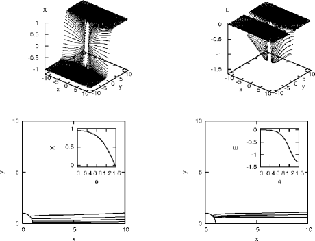
Figure 1: The field X (left panels) and the quantity E (right panels) for the $\phi^{4}$ potential and the cosmological AdS black hole. Isolines on bottom panels are drawn for $0.2$, $0.4$, $0.6$ and $0.8$ for the field X and for $-0.1$, $-0.2$, $-0.3$ and $-0.4$ for the energy. Inlets in bottom plots show the value of the fields on the black hole horizon. Black hole has $M=1.0$, $Q=0.1$, $l=1.0$ and the domain width is $w=1.0$.

Figure 2: Same as Fig. 1, but for $l=2.0$

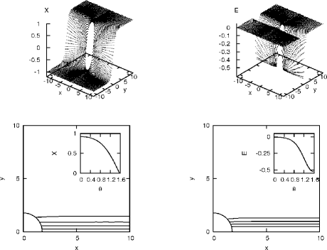
Figure 3: Same as Fig. 1, but for $l=5.0$

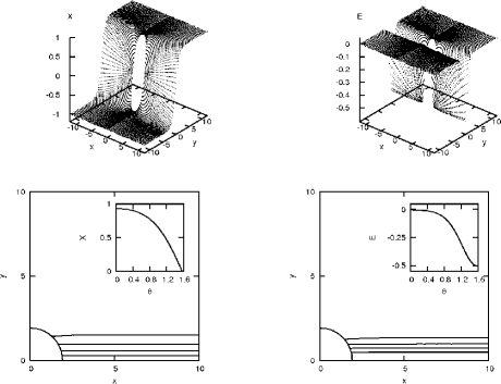
Figure 4: Same as Fig. 1, but for $l=10.0$

Figures 5-8 depict the solutions of equations of motion for scalar field $X$ and show changes of $E$, for AdS black hole with sine-Gordon potential. The mass of the black hole under consideration one has equal to $M=1.0$ and the cosmological parameters are chosen respectively to be $1$, $2$, $5$ and $10$. The width of the domain wall was taken to be $1$.

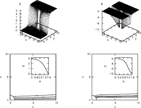
Figure 5: The field X (left panels) and the quantity E (right panels) for the sine-Gordon potential and the cosmological AdS black hole. Isolines on bottom panels are drawn for $0.2\pi$, $0.4\pi$, $0.6\pi$ and $0.8\pi$ for the field X and for $-0.5$, $-1.5$, $-2.5$ and $-3.5$ for the energy. Inlets in bottom plots show the value of the fields on the black hole horizon. Black hole has $M=1.0$, $Q=0.0$, $l=1.0$ and the domain width is $w=1.0$.

Figure 6: Same as Fig. 5, but for $l=2.0$

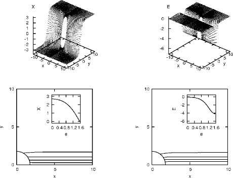
Figure 7: Same as Fig. 5, but for $l=5.0$

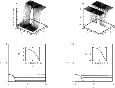
Figure 8: Same as Fig. 5, but for $l=10.0$

On the other hand, Figures 9-10 show the behaviour of the scalar field $X$ on the black hole axis both for $\phi^{4}$ and sine-Gordon potentials.

Figure 9: Values of the field X on the black hole axis for $l=1,2,3,5,10$ – solid curves from left to right, respectively. Dashed line represents the solution for $l=\inf$. Rest of the parameters are the same as in Figure 1.

Figure 10: Same as Fig. 9, but for sine-Gordon potential.

Figure 11 presents values of the ratio $Q^{2}/M^{2}$ for which the black hole under considerations becomes extreme. We consider it as a function of the cosmological parameter $l$ and plots are made for different values of the black hole masses, i.e., $M=1,~{}10,~{}100,~{}1000$.

Figure 11: $Q^{2}/M^{2}$ as a function of the cosmological parameter $l$ for extreme black hole. The curves are for $M=1,10,100,1000$, from left to right.

In Figs. 12-15 we plotted the values of $X$ and the parameter $E$ for extremal black holes. It revealed that the field expulsion takes place only when the value of $\alpha$ parameter is smaller than $2.0$. The same situation we ancountered in the case of RN black holes Moderski and Rogatko (2004). On the contrary, in the case of extremal dilaton black hole domain wall system one gets always expulsion of the scalar field Rogatko (2001); Moderski and Rogatko (2003). It was revealed that the simplest generalization of Einstein-Maxwell theory by adding a massless dilaton field dramatically changes the structure and properties of extremal black holes. Figure 12 depicts the value of the scalar field $X$ and $E$ for $\alpha\sim 0.6$ and for $\phi^{4}$-potential. In Fig. 13 we change the value of $\alpha$. Now it is equal to $6.6$. The results depicted in Figs. 14-15 are valid for sine-Gordon potential and $\alpha=0.6$ and $6.6$, respectively.

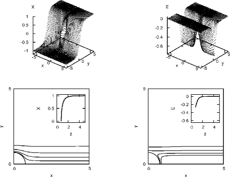
Figure 12: The field X (left panels) and E (right panels) for the $\phi^{4}$ potential and the extremal cosmological AdS black hole. Isolines on bottom panels are drawn for $0.2$, $0.4$, $0.6$ and $0.8$ for the field X and for $-0.5$, $-1.5$, $-2.5$ and $-3.5$ for E. Inlets in bottom plots show the value of the fields on the black hole horizon. Black hole has $M=1.0$, the cosmological parameter $l=1.0$ and $\alpha\approx 0.6$.

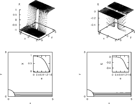
Figure 13: Same as Fig. 12, but for $\alpha\approx 6.6$.

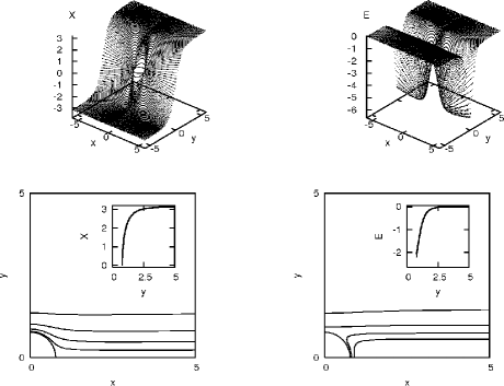
Figure 14: Same as Fig. 12, but for sine-Gordon potential.

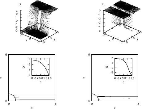
Figure 15: Same as Fig. 14, but for $\alpha\approx 6.6$.

In Figs. 16-17 we show the $X$ and $E$ values for anti-Nariai black hole with $R_{0}=1$ and $K_{0}=1/2$ both for $\phi^{4}$ and sine-Gordon potentials. In Ref. Rogatko (2004) the charged Nariai and anti-Nariai domain wall systems were studied. Due to the complication of equations of motion the simple arguments concerning the problem of expulsion of scalar field were given. However, the present analysis reveals the fact that there is no expulsion for the anti-Nariai case. Nevertheless, in the vicinity of the event horizon one obtains very small value of the field $X$.

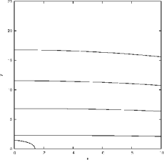
Figure 16: X field configuration for anti-Nariai black hole $R_{0}=1.0$ and $K_{0}=1/2$ for $\phi^{4}$ potential. Left panel shows the value of the field, and right panel presents $0.2,0.4,0.6,0.8$ contours.

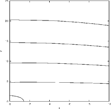
Figure 17: Same as Fig. 16, but for sine-Gordon potential. Contours on the right panel are for $0.2\pi,0.4\pi,0.6\pi,0.8\pi$.

V Conclusions

Our considerations were devoted to studies of AdS black hole domain wall system. As in our previous works Moderski and Rogatko (2003, 2004) the domain wall’s equations of motion were built from a self-interacting real scalar field with a symmetry breaking potential having a discrete set of degenerate minima. In our considerations we took into account two kinds of potentials, i.e., $\phi^{4}$ and sine-Gordon potential. We used in numerical analysis simultaneously over-relaxation method Press et al. (1992) to solve equations of motion for scalar field $X$ fulfilling the certain conditions on the black hole event horizon. The solutions of equations of motion depended on the parameter $w=1/\sqrt{{\lambda}}\eta$ which was responsible for the domain wall thickness and the cosmological parameter $l$. We paid a special attention to extreme black hole solutions. As in the case of RN domain wall systems studied in Ref. Moderski and Rogatko (2004) the expulsion of scalar fields from AdS black hole is dependent on the parameter $\alpha={r_{EH}^{2}/w^{2}}$. The expulsion takes place when $\alpha<2$, while for $\alpha>2$ the domain wall can penetrate the extremal black hole. We confront the numerical studies of anti-Nariai black hole domain wall system to our very simple analytical analysis of the problem. Contrary to simple analytical arguments given in Ref. Rogatko (2004) we revealed that numerical studies contradicts this suggestion. There is no expulsion of scalar field in this case.