Quantum Nature of the Big Bang: Improved dynamics

Abstract

An improved Hamiltonian constraint operator is introduced in loop quantum cosmology. Quantum dynamics of the spatially flat, isotropic model with a massless scalar field is then studied in detail using analytical and numerical methods. The scalar field continues to serve as ‘emergent time’, the big bang is again replaced by a quantum bounce, and quantum evolution remains deterministic across the deep Planck regime. However, while with the Hamiltonian constraint used so far in loop quantum cosmology the quantum bounce can occur even at low matter densities, with the new Hamiltonian constraint it occurs only at a Planck-scale density. Thus, the new quantum dynamics retains the attractive features of current evolutions in loop quantum cosmology but, at the same time, cures their main weakness.

I Introduction

The spatially flat, isotropic model was recently investigated in detail in the setting of loop quantum cosmology (LQC) aps2 . (For a brief summary of results, see aps1 .) That investigation introduced a conceptual framework and analytical and numerical tools to construct the physical sector of the quantum theory. These methods enabled one to systematically explore the effects of quantum geometry both on the gravitational and matter sectors and to extend the previous results in LQC.

If the only matter source is a massless scalar field, every classical solution has a singularity which, furthermore, persists in the Wheeler-DeWitt theory. Therefore, to bring out effects which can be unambiguously attributed to the quantum nature of geometry underlying LQC, this model was analyzed in detail in aps1 ; aps2 . The analysis led to the following results: i) the scalar field was shown to serve as an internal clock, thereby providing a detailed realization of the ‘emergent time’ idea; ii) the physical Hilbert space, Dirac observables and semi-classical states were constructed rigorously; and, iii) the Hamiltonian constraint was solved numerically to show that in the backward evolution of states which are semi-classical at late times, the big bang is replaced by a quantum bounce. Furthermore, thanks to the non-perturbative, background independent methods, unlike in other approaches the quantum evolution is deterministic across the deep Planck regime.

These results are attractive and add to the growing evidence mb1 ; abl ; mbrev suggesting that the quantum geometry effects of loop quantum gravity (LQG) hold a key to many long standing questions. Control over the physical sector of the theory and availability of numerical methods also enabled to us to analyze the physics of the bounce in greater detail than could be done in previous investigations. These details enriched our understanding of both the semi-classical and deep Planck regimes. However, they also brought out a serious limitation of the framework: the critical value $\rho_{\mathrm{crit}}$ of the matter density at which the bounce occurs can be made arbitrarily small by increasing the momentum $p_{\phi}$ of the scalar field (which is a constant of motion). Now, large values of $p_{\phi}$ are permissible and even preferred for semi-classical considerations at late times. Since it is physically unreasonable to expect quantum corrections to significantly modify classical predictions at low matter densities, this limitation is a serious drawback. Indications of such problems had appeared also in some of the earlier results based on effective equations (see, e.g., dh2 ; mbrev ). However, since the approximations inherent to effective equations break down in the deep Planck regime, one did not have an a priori reason to believe that these were consequences of the underlying quantum equations of LQC, rather than artifacts of approximation schemes. The analysis of aps2 unambiguously showed that the problem lies with the quantum equations themselves. Thus, while the quantum evolution predicted by the existing LQC constraint operator has a number of attractive features, it has one major weakness. A key question then is whether one can change the definition of the constraint operator in a subtle way so that this problem is overcome, but the attractive features of the evolution are all preserved.

As reported in aps2 ; aps1 , the answer is in the affirmative. The purpose of this paper is to justify this assertion by providing the detailed construction of the new Hamiltonian constraint and analyzing the resulting quantum dynamics. We will find that the required change is in fact physically well motivated and conceptually quite compelling.

The main ideas can be summarized as follows. Recall that, to obtain the expression of the quantum constraint, one has to first introduce an operator representing curvature of the gravitational connection. Now, a key feature of LQC —inherited directly from full loop quantum gravity (LQG)— is that while there are well defined quantum analogs of holonomies, there is no operator corresponding to the connection itself alrev ; crbook ; ttbook . Thus, one is naturally led to define the curvature operator in terms of holonomies. In the classical theory, curvature can be expressed as a limit of the holonomies around a loop as the area enclosed by the loop shrinks to zero. In quantum geometry, however, one can not continuously shrink the loop to zero area; there is a smallest non-zero area eigenvalue, or an ‘area gap’ $\Delta$ rs ; almmt ; al5 . The physical idea then is to incorporate the existence of the mass gap $\Delta$ abl in the limiting procedure. However, in the existing definition of the quantum constraint, this physical idea was mathematically implemented in a rather indirect manner. Initially, it was meant to be only a first step to gain a qualitative understanding of dynamics within LQC. Nonetheless, as more and more physically appealing features of this dynamics were discovered, the constraint operator obtained by this procedure was taken more and more seriously and constituted the basis of a number of approximation schemes and effective descriptions.

The new Hamiltonian constraint introduced in this paper is based on the same principles but the curvature operator is now constructed by a more direct implementation of the underlying physical ideas. The structure of the final constraint operator does change significantly but, when suitably recast, its form is actually somewhat simpler. Furthermore, it has additional conceptually attractive features. For example, its Wheeler-DeWitt (WDW) limit naturally comes with the ‘covariant factor ordering’ of that theory. Once the new constraint is introduced, we apply analytical and numerical methods of aps2 to extract physical predictions from the theory. Specifically, we will build the physical Hilbert space ${\cal H}_{\rm phy}$ from solutions to the new quantum constraint, introduce on it a complete family of Dirac observables, construct suitable families of states which are semi-classical at ‘late times’ (e.g., ‘now’), and numerically evolve them back in time. As in aps2 , we will find that in this backward evolution, the big bang is again replaced by the quantum bounce. Qualitative features of the evolution are very similar to those observed in aps2 , except that the big bounce occurs precisely when the matter density enters the Planck regime, irrespective of the value of $p_{\phi}$ and other initial conditions.

To summarize, the Hamiltonian constraint will be improved by implementing the physical idea of abl in a more satisfactory manner. The resulting dynamics will retain the attractive features of the older quantum evolution but free it from its main drawback. This rather delicate interplay between physics and mathematics is both interesting and instructive. We wish to emphasize however that the present procedure still retains a basic limitation of the existing treatments: the Hamiltonian constraint is not systematically derived from the full theory. Indeed, this important task can not yet be undertaken because there is no unambiguous Hamiltonian constraint in the full theory which can serve as the natural starting point for a systematic reduction.

The organization of this paper parallels that of aps2 and we use the same notation. We direct the reader to that paper for motivations as well as further technical details. In Section II we introduce the new Hamiltonian constraint operator. In Section III we discuss the WDW  theory that results when one ignores the effects of quantum geometry. As in aps2 , we find that the singularity is not resolved in that limit. In Section IV we return to LQC and construct the physical sector of the theory. Quantum states which are semi-classical at ‘late times’ are then numerically evolved backwards in Section V. We find that the classical big bang is replaced by a quantum bounce which occurs when the matter is compressed enough to acquire a density of the Planck scale. Thus, in the deep Planck regime, quantum geometry has the effect of making gravity strongly repulsive. A key virtue of the new constraint operator is that these effects are completely negligible when the matter density is significantly smaller than the Planck density. Section VI summarizes the main results and briefly discusses possible extensions. While our detailed analysis is restricted to a specific and rather simple model, the key ideas behind the construction of the new constraint operator can be applied much more generally. This is illustrated in Appendix A where we allow for the presence of a cosmological constant. (Other models will be discussed also by other authors in forthcoming papers.) Appendix B discusses conceptual issues that are especially relevant to approximation schemes used in constructing effective equations.

A brief overview of LQG emphasizing these developments in LQC can be found in aaparis .

II The improved Constraint Operator

This section is divided into three parts. In the first two we introduce the key new elements and in the third we put them together to construct the new Hamiltonian constraint operator.

II.1 Strategy

Let us first collect the required background material and notation. (For details, see abl ; aps2 .) In a systematic Hamiltonian treatment of spatially flat, isotropic models, one has to first introduce an elementary cell ${\cal V}$ and restricts all integrations to this cell. Fix a fiducial flat metric ${}^{o}\!q_{ab}$ and denote by $V_{o}$ the volume of the elementary cell ${\cal V}$ in this geometry. The gravitational phase space variables —the connections $A_{a}^{i}$ and the density weighted triads $E^{a}_{i}$— can be expressed as:

$$A_{a}^{i}=c\,V_{o}^{-\frac{1}{3}}{}^{o}\!\omega_{a}^{i},\quad{\rm and}\quad E^{a}_{i}=p\,V_{o}^{-\frac{2}{3}}\sqrt{q_{o}}\,\,{}^{o}\!e^{a}_{i}$$ (1)

where $({}^{o}\!\omega_{a}^{i},{}^{o}\!e^{a}_{i})$ are a set of orthonormal co-triads and triads compatible with ${}^{o}\!q_{ab}$ and adapted to the edges of the elementary cell ${\cal V}$. Thus, the symmetry reduced gravitational phase space is only 2-dimensional, coordinatized by the pair $(c,p)$. Thanks to the availability of the fiducial cell ${\cal V}$, the coordinates $(c,p)$ are insensitive to the choice of the fiducial metric, i.e., remain unchanged under the rescaling ${}^{o}\!q_{ab}\rightarrow\alpha^{2}{}^{o}\!q_{ab}$. The fundamental Poisson bracket is given by:

$$\{c,\,p\}=\frac{8\pi G\gamma}{3}$$ (2)

where $\gamma$ is the Barbero-Immirzi parameter. The gravitational part of the Hamiltonian constraint can be written as:

$$C_{\mathrm{grav}}=-\gamma^{-2}\int_{\cal V}d^{3}x\,\varepsilon_{ijk}\,e^{-1}E^{ai}E^{bj}\,\,F_{ab}^{k}=-\frac{6}{\gamma^{2}}\,c^{2}\sqrt{p}$$ (3)

where $e:=\sqrt{|\mathrm{det}E|}$.

In quantum theory, following Dirac, one first constructs a kinematical description. The Hilbert space ${\cal H}_{\rm kin}^{\rm grav}$ is the space $L^{2}(\mathbb{R}_{\rm Bohr},d\mu_{\rm Bohr})$ of square integrable functions on the Bohr compactification of the real line. To specify states concretely, it is convenient to work with the representation in which the operator $\hat{p}$ is diagonal. Eigenstates of $\hat{p}$ are labelled by a real number $\mu$ and satisfy the orthonormality relation:

$${\langle\mu_{1}\,|\,\mu_{2}\rangle}=\delta_{{\mu_{1}},\,{\mu_{2}}}\,.$$ (4)

Since the right side is the Kronecker delta rather than the Dirac delta distribution, a typical state in ${\cal H}_{\rm kin}^{\rm grav}$ can be expressed as a countable sum; $|\Psi\rangle=\sum_{n}c^{(n)}|\mu_{n}\rangle$ where $c^{(n)}$ are complex coefficients and the inner product is given by

$$\langle\Psi_{1}|\Psi_{2}\rangle=\sum_{n}\,\bar{c}_{1}^{(n)}\,c_{2}^{(n)}~{}.$$ (5)

The fundamental operators are $\hat{p}$ and $\widehat{\exp i\lambda(c/2)}$:

$$\hat{p}\,|\mu\rangle=\frac{8\pi\gamma{\ell}_{\rm Pl}^{2}}{6}\,\mu\,|\mu\rangle\quad{\rm and}\quad\widehat{\exp{\frac{i\lambda c}{2}}}\,|\mu\rangle=|\mu+\lambda\rangle$$ (6)

where $\lambda$ is any real number. Since the holonomy $h_{k}^{(\lambda)}$ of the gravitational connection $A_{a}^{i}$ along a line segment $\lambda\,{}^{o}\!e^{a}_{k}$ is given by:

$${h^{(\lambda)}_{k}}=\cos{\scriptstyle\frac{\lambda c}{2}}\,\mathbb{I}+2\sin{\scriptstyle\frac{\lambda c}{2}}\,\tau_{k}$$ (7)

the corresponding holonomy operator has the action:

$$\hat{h}^{(\lambda)}_{k}\,|\mu\rangle=\frac{1}{2}\,\left(|\mu+\lambda\rangle+|\mu-\lambda\rangle\right)\mathbb{I}+\frac{1}{i}\,\left(|\mu+\lambda\rangle-|\mu-\lambda\rangle\right)\tau_{k}~{}.$$ (8)

However, just as there is no operator corresponding to the connection itself in full LQG almmt ; alrev ; crbook ; ttbook , there is no operator $\hat{c}$ on ${\cal H}_{\rm kin}^{\rm grav}$ afw ; abl .

To describe quantum dynamics, we have to first introduce a well-defined operator on ${\cal H}_{\rm kin}^{\rm grav}$ representing the Hamiltonian constraint $C_{\rm grav}$. Since there is no operator corresponding to $c$ itself, we return to the integral expression of the constraint from the full LQG:

$$C_{\mathrm{grav}}=-\gamma^{-2}\int_{\cal V}d^{3}x\,\varepsilon_{ijk}\,e^{-1}E^{ai}E^{bj}\,F_{ab}^{i}~{}.$$ (9)

For passage to quantum theory, we first need to express this classical constraint in terms of the elementary variables $p$ and $h_{k}^{(\lambda)}$ which have unambiguous quantum analogs. As in the full theory tt ; ttbook , the term involving triads can be written as

$$\varepsilon_{ijk}\,e^{-1}\,E^{aj}E^{bk}\,=\,\sum_{k}\frac{({\rm sgn}\,p)}{2\pi\gamma G\lambda\,V_{o}^{\frac{1}{3}}}\,\,{}^{o}\!\varepsilon^{abc}\,\,{}^{o}\!\omega^{k}_{c}\,\,{\rm Tr\,}\left(h_{k}^{(\lambda)}\,\{h_{k}^{(\lambda)}{}^{-1},V\}\,\tau_{i}\right)$$ (10)

where $V=|p|^{3/2}$ is the volume of elementary cell ${\cal V}$ in the physical metric determined by $p$ and the holonomy $h_{k}^{(\lambda)}$ is evaluated along the segment $\lambda\,{}^{o}\!e^{a}_{k}$ (i.e., a segment of oriented length $\lambda$ along the $k$th edge of the elementary cell ${\cal V}$). Note that this identity holds for any choice $\lambda$, even when it is allowed to be a function of $p$. Let us allow for this possibility and fix the appropriate $\lambda$ at the end.

For the field strength $F_{ab}^{i}$, we use the standard strategy employed in gauge theories. Consider a square $\Box_{ij}$ in the $i$-$j$ plane spanned by a face of the elementary cell, each of whose sides has length $\lambda V_{o}^{1/3}$ with respect to the fiducial metric ${}^{o}\!q_{ab}$. Then, ‘the $ab$ component’ of the curvature is given by:

$$F_{ab}^{k}\,=\,-2\,\lim_{Ar_{\Box}\rightarrow 0}\,\,{\rm Tr\,}\,\left(\frac{h^{(\lambda)}_{\Box_{ij}}-1}{\lambda^{2}V_{o}^{2/3}}\right)\,\,\tau^{k}\,{}^{o}\!\omega^{i}_{a}\,\,{}^{o}\!\omega^{j}_{b}\,.$$ (11)

Here $Ar_{\Box}$ is the area of the square under consideration, and the holonomy $h^{(\mu_{o})}_{\Box_{ij}}$ around the square $\Box_{ij}$ is just the product of holonomies (7) along the four edges of $\Box_{ij}$:

$$h^{(\lambda)}_{\Box_{ij}}=h_{i}^{(\lambda)}h_{j}^{(\lambda)}(h_{i}^{(\lambda)})^{-1}(h_{j}^{(\lambda)})^{-1}\,.$$ (12)

Combining Eqs. (10) and (11), $C_{\mathrm{grav}}$ can be written as

$$C_{\mathrm{grav}} = \lim_{Ar_{\square}\rightarrow 0}C_{\mathrm{grav}}^{(\lambda)}\quad\mathrm{where}$$

$$C_{\mathrm{grav}}^{(\lambda)} = -\frac{4\,\mathrm{sgn}(p)}{8\pi\gamma^{3}\lambda^{3}G}\,\sum_{ijk}\,\varepsilon^{ijk}\,\mathrm{Tr}\left(h_{i}^{(\lambda)}h_{j}^{(\lambda)}(h_{i}^{(\lambda)})^{-1}(h_{j}^{(\lambda)})^{-1}h_{k}^{(\lambda)}\{(h_{k}^{(\lambda)})^{-1},\,V\}\right)$$ (13)

$$= \sin\lambda c\left[-\,\frac{4}{8\pi G\gamma^{3}}\frac{{\rm sgn}(p)}{\lambda^{3}}\,\sum_{k}{\rm Tr\,}\tau_{k}h_{k}^{(\lambda)}\,\{(h_{k}^{(\lambda)})^{-1},\,V\}\right]\sin\lambda c$$

where in the last step we have used a symmetric ordering of the three terms for later convenience. Since the constraint is now expressed in terms of elementary variables which have unambiguous quantum analogs, it is straightforward to write down the quantum operator $\hat{C}_{\mathrm{grav}}^{(\lambda)}$. However, the limit $Ar_{\Box}\rightarrow 0$ of this operator does not exist. This is not accidental; had the limit existed, there would be a well-defined local operator corresponding to the curvature $F_{ab}^{i}$ and we know that even in full LQG, while holonomy operators are well defined, there are no local operators representing connections and curvatures. This feature is intimately intertwined with the quantum nature of Riemannian geometry of LQG. The viewpoint in LQC is that the failure of the limit to exist is a reminder that there is an underlying quantum geometry where eigenvalues of the area operator are discrete, whence there is a smallest non-zero eigenvalue, $\Delta$, i.e., an area gap. Thus, quantum geometry is telling us that, on physical grounds, it is inappropriate to let $Ar_{\Box}$ go to zero; the ‘correct’ procedure must take into account the existence of the area gap.

Up to this stage, we have followed the standard LQC reasoning, first introduced in abl . The difference comes in the implementation of the above idea. The viewpoint we now adopt is that since quantization of area refers to physical geometries, we should shrink the loop $\Box_{ij}$ till the area enclosed by it, as measured by the physical metric $q_{ab}$, reaches the value $\Delta$. Since the physical area of faces of the elementary cell is $|p|$ and since each side of $\Box_{ij}$ is $\lambda$ times the edge of the elementary cell, we are led to choose for $\lambda$ a specific function $\bar{\mu}(p)$, given by

$$\bar{\mu}^{2}\,\,|p|\,=\,\Delta\,\equiv\,(2\sqrt{3}\pi\gamma)\,{\ell}_{\rm Pl}^{2}$$ (14)

While $\bar{\mu}$ is a non-trivial function on the phase space, its analog $\mu_{o}$ in the existing LQC treatments was required to be a constant. Technically, this contrast turns out to be important. If we write the quantum constraint using the $|\mu\rangle$ basis, the constraint operator of abl ; aps2 is a difference operator with uniform step size, given by $4\mu_{o}$. In this basis the action of the new quantum constraint would be again given by a difference operator, but the step size now depends on the state $|\mu\rangle$ it operates on. This difference turns out to be subtle enough to remove the major weakness of the current LQC constraint operator, while retaining its physically desirable features. Conceptually, the new strategy has important ramifications for the fundamental curvature operator. In both treatments, it is non-local. However, while the non-local operator used in the existing literature depends only on the connection, the non-local operator introduced here depends both on the connection and the geometry. In the classical limit, effects of quantum geometry are negligible and the classical limits of both operators yield the standard expression of the curvature $F_{ab}$.

Finally, some heuristics involving full LQG can be used rather effectively to bring out the physical difference between the two strategies. In the sector of full LQG consisting of a small but a finite neighborhood of homogeneous isotropic cosmologies, one should be able to carry out partial gauge fixing, enabling one to speak of 3-metrics (rather than their equivalence classes under diffeomorphisms). Let us consider quantum geometry states based on graphs and for simplicity focus on the fixed fiducial cell. Then, one would expect that, as the scale factor $a$ grows, the number $N$ of vertices in the graph contained in the fiducial cell would grow as $N=K_{o}a^{3}$ for some constant $K_{o}$. In the Hamiltonian constraint of full LQG, the operator $F_{ab}$ would have to be evaluated at these vertices. A natural procedure is to introduce an ‘elementary cube’ around each vertex and calculate the holonomy around the faces of that cube. Since the number $N$ of elementary cubes contained in the fiducial cell increases as $a$ grows, the area of their faces, as measured by the fixed fiducial metric would decrease as $Ar_{\rm ele}^{o}\sim(1/N)^{2/3}\sim 1/|p|$. Hence, as measured by the fiducial metric, the length of each edge of the face around which the holonomy is evaluated would go as $1/\sqrt{|p|}$ — i.e. precisely as $\bar{\mu}$. Thus the functional dependence of $\bar{\mu}$ on $\mu$ can be thought of as the remnant left behind by the sector of the full theory of interest to cosmology, on the mini-superspace considered in this paper. Fixing the edge length to be $\mu_{o}$, i.e., making it state independent, amounts to ignoring the ‘creation of new vertices’ that one expects to accompany the expansion of the universe. These considerations complement ideas recently advocated by Bojowald to incorporate inhomogeneities in LQC boj-pc .

II.2 The operator $\widehat{\exp i(\bar{\mu}c/2)}$

Having fixed $\lambda$ to be the specific function $\bar{\mu}(p)$, we are now led to write the expression of the quantum constraint by replacing $\lambda$ in the right side of (II.1) by $\bar{\mu}$, the holonomies and the volume functions by corresponding operators, and the Poisson bracket by $1/i\hbar$ times the commutator. However, to carry out this task, we first need to define the operators $\widehat{\cos(\bar{\mu}c/2)}$ and $\widehat{\sin(\bar{\mu}c/2)}$, i.e. the operator $\widehat{\exp i(\bar{\mu}c/2)}$. This task is a somewhat subtle because i) there is no operator corresponding to $c$ and hence to $\bar{\mu}c$, and, ii) since $\bar{\mu}$ is a function of $p$, ${\exp i(\bar{\mu}c/2)}$ can not be expressed as a function of the ‘elementary variables’ —$p$ and $\exp i(kc/2)$ where $k$ is a constant.

However, in this task we are aided by geometric considerations. Let us begin with states $\tilde{\Psi}(\mu)$ in the Schrödinger Hilbert space, $L^{2}(\mathbb{R},d\mu)$. For any real constant $k$ we have:

$$\widehat{e^{i\frac{kc}{2}}}\,\tilde{\Psi}(\mu)\,=\,\tilde{\Psi}(\mu+k)\,\equiv\,e^{k\frac{\textrm{d}}{\textrm{d}\mu}}\,\tilde{\Psi}(\mu)\,.$$ (15)

Thus, the action of the operator is to drag the state along the vector field $k\frac{\textrm{d}}{\textrm{d}\mu}$. Now, the 1-parameter family of diffeomorphisms generated by the vector field $\textrm{d}/\textrm{d}\mu$ has a well-defined action also on the Hilbert space ${\cal H}_{\rm kin}^{\rm grav}$ now under consideration. Therefore, Eq (15) holds also for states $\tilde{\Psi}(\mu)$ in ${\cal H}_{\rm kin}^{\rm grav}$ provided $\exp k\textrm{d}/\textrm{d}\mu$ is interpreted simply as the operator that drags the state a unit affine parameter distance along the vector field $k\frac{\textrm{d}}{\textrm{d}\mu}$. This suggests that it is natural to set

$$\widehat{e^{i\frac{\bar{\mu}c}{2}}}\,\tilde{\Psi}(\mu)=e^{\bar{\mu}\frac{\textrm{d}}{\textrm{d}\mu}}\,\tilde{\Psi}(\mu)$$ (16)

so the right side would be the image of $\tilde{\Psi}$ under the finite diffeomorphism obtained by moving a unit affine parameter distance along the integral curve of the vector field $\xi=\bar{\mu}\frac{\textrm{d}}{\textrm{d}\mu}$. The affine parameter $v$ along this vector field is given by:

$$v=K\,{\rm sgn}(\mu)\,|\mu|^{\frac{3}{2}},\quad{\rm where}\quad K=\frac{2\sqrt{2}}{3\sqrt{3\sqrt{3}}}$$ (17)

Although the geometrical meaning of this action of $\widehat{\exp i(\bar{\mu}c/2)}$ is simple, since $v$ is a rather complicated function of $\mu$, its expression in the $\mu$-representation is complicated:

$$\widehat{e^{i\frac{\bar{\mu}c}{2}}}\,\tilde{\Psi}(\mu)=\tilde{\Psi}({\rm sgn}(\tilde{\mu})\mid\tilde{\mu}\mid^{\frac{2}{3}}),\quad{\rm where}\quad\tilde{\mu}={\rm sgn}(\mu)\,|\mu|^{\frac{3}{2}}+\frac{1}{K}\,$$ (18)

However, it is well-defined because $v(\mu)$ is an invertible (and $C^{1}$) function of $\mu$. Furthermore, for $\mu\gg 1$, the action reduces to the form

$$\widehat{e^{i\frac{\bar{\mu}c}{2}}}\,\tilde{\Psi}(\mu)\approx\tilde{\Psi}(\mu+\bar{\mu})$$ (19)

familiar from the ‘standard’ LQG analysis where $\bar{\mu}$ is replaced by a constant $\mu_{o}$ (see Eq (15)). However, as is clear from the exact expression (18), this form with a ‘simple displacement’ of the argument is highly inaccurate for small $\mu$.

The complicated action of $\widehat{\exp i(\bar{\mu}c/2)}$ just reflects the fact that the variable $\mu$ determined by eigenvalues of $\hat{p}$ is not well-adapted to the vector field $\xi$. Let us therefore change the basis $|\mu\rangle$ to $|v\rangle$. This basis is more directly adapted to the volume operator $\hat{V}$ (associated with the elementary cell ${\cal V}$):

$$\hat{V}|v\rangle=(\frac{8\pi\gamma}{6})^{\frac{3}{2}}\,\frac{|v|}{K}\,{\ell}_{\rm Pl}^{3}\,|v\rangle$$ (20)

(It follows from (17) that, like $\mu$, $v$ is dimensionless.) These kets also constitute an orthonormal basis in ${\cal H}_{\rm kin}^{\rm grav}$: ${\langle v_{1}\,|\,v_{2}\rangle}=\delta_{v_{1},\,v_{2}}$. The two bases are of course closely related because $\hat{V}$ and $\hat{p}$ are just functions of one another. In terms of representations, we can simply set $\Psi(v)=\tilde{\Psi}(\mu)$. In the $v$-representation, the action of $\widehat{\exp i(\bar{\mu}c/2)}$ is extremely simple :

$$\widehat{e^{i\frac{\bar{\mu}c}{2}}}\,\Psi(v)=\Psi(v+1)$$ (21)

Therefore, in what follows we will use the $v$ representation. Many of the expressions obtained using the new constraint will then have a form rather similar to those obtained in abl ; aps2 . But it is important to keep in mind that while those expressions were written in the $\mu$ representation, the ones in this paper are written in the $v$-representation. This difference is a key reason why the present Hamiltonian constraint is free of the drawback of the one used in the literature so far.

Note that the operator $\widehat{\exp i(\bar{\mu}c/2)}$ is unitary. We can extend the definition in the obvious manner: By setting

$$\widehat{e^{ik\frac{\bar{\mu}c}{2}}}\,\Psi(v)=\Psi(v+k)$$ (22)

for any constant $k$, we obtain a unitary representation on ${\cal H}_{\rm kin}^{\rm grav}$ of the 1-parameter group of diffeomorphisms generated by the vector field $\xi$. On the classical phase space, the function $\bar{\mu}c/2$ generates a 1-parameter family of (finite) canonical transformations. It is precisely the lift to the phase space of the 1-parameter group of diffeomorphisms on the $p$ or $\mu$ space, generated by the vector field $\bar{\mu}\textrm{d}/\textrm{d}\mu$. The action of $\widehat{\exp i(\bar{\mu}c/2)}$ simply promotes this relation to the quantum theory.

Remark: While the geometric interpretation of the action of $\widehat{\exp i(\bar{\mu}c/2)}$ makes its definition quite natural, one might nonetheless ask for the relation between our factor ordering and that normally used. We will now argue that the choice we have specified in fact originates in ordinary quantum mechanics.

Consider 1-d Schrödinger quantum mechanics, where states $\tilde{\Psi}(x)$ are generally taken to be functions in $L^{2}(\mathbb{R},\textrm{d}x)$. Consider a function $f(x)p$ on the classical phase space. The canonical transformation it generates is again the lift to the phase space of the diffeomorphism generated by the vector field $\xi=f(x)\frac{\textrm{d}}{\textrm{d}x}$ on the configuration space (i.e., the x-axis). One would expect that this geometric action would be carried over also to quantum theory. Is this in fact the case? In the textbook treatments one does not take into account such geometric considerations but constructs a self-adjoint operator $\widehat{(fp)}:=(\hbar/2i)\,(f\,\frac{\textrm{d}}{\textrm{d}x}+\frac{\textrm{d}}{\textrm{d}x}\,f)$ using a symmetric ordering. Its action $\widehat{(fp)}\tilde{\Psi}=(\hbar/i)\,(f\,\frac{\textrm{d}}{\textrm{d}x}\tilde{\Psi}+\frac{1}{2}\,\frac{\textrm{d}}{\textrm{d}x}\,f\,\tilde{\Psi})$ does not correspond to the Lie-derivative of $\tilde{\Psi}$ with respect to the vector field $\xi$, which is captured just in the first term. (The second term, $\frac{1}{2}\,\frac{\textrm{d}}{\textrm{d}x}\,f\,\tilde{\Psi}$, multiplies $\tilde{\Psi}$ by the divergence of the vector field $\xi$, i.e., by the Lie-derivative of the Lebesgue measure with respect to $\xi$.) Hence, the action of the 1-parameter group of unitary transformations $\hat{U}(\lambda):=\exp i\widehat{(fp)}$ on wave functions $\tilde{\Psi}(x)$ is different from that of the diffeomorphisms generated by $\xi$. However, this is simply because the Lebesgue measure $\textrm{d}x$ fails to be invariant under the diffeomorphism.

Let us represent quantum states by densities $\Psi$ of weight 1/2 —or, more precisely, half-forms— so that the scalar product is given simply by $(\Psi_{1},\Psi_{2})=\int_{\mathbb{R}}\bar{\Psi}_{1}\,\Psi_{2}$ without the need of a measure. (Thus, $\bar{\tilde{\Psi}}_{1}\tilde{\Psi}_{2}\textrm{d}x\sim\bar{\Psi}_{1}\Psi_{2}$. For details, see, e.g., nmjw .) On these half forms, the action of $\widehat{(fp)}$ is precisely that of a Lie derivative; $\widehat{(fp)}\,\Psi=(\hbar/i)\,{\cal L}_{\xi}\Psi$. Therefore, the action of the unitary transformation $U(\lambda)$ is given by:

$$\hat{U}(\lambda)\Psi(v)\,=\,\Psi(v+\lambda\hbar)$$

where $v$ is the affine parameter of the vector field $\xi$ on $\mathbb{R}$. Thus, the initial geometric expectation is indeed realized if one proceeds with the standard factor ordering from Schrödinger quantum mechanics, but represents states by half forms. In the polymer representation the measure is invariant under the action of any diffeomorphism on the $\mu$-axis. Hence the additional ‘divergence term’ is unnecessary. In this sense, states in ${\cal H}_{\rm kin}^{\rm grav}$ are analogs of densities of weight 1/2 —or, half forms— in the Schrödinger representation.

II.3 Expression of the constraint operator

We can now collect the results of the last two sub-sections to obtain the quantum constraint operator starting from the classical expression (II.1). We have:

$$\hat{C}_{\mathrm{grav}} = \,\sin(\bar{\mu}c)\,\,\bigg{[}\frac{24i\,\mathrm{sgn}(\mu)}{8\pi\gamma^{3}\bar{\mu}^{3}{\ell}_{\rm Pl}^{2}}\,\left(\sin\left(\frac{\bar{\mu}c}{2}\right)\hat{V}\cos\left(\frac{\bar{\mu}c}{2}\right)-\cos\left(\frac{\bar{\mu}c}{2}\right)\hat{V}\sin\left(\frac{\bar{\mu}c}{2}\right)\right)\bigg{]}\sin(\bar{\mu}c)$$ (23)

$$=: \sin(\bar{\mu}c)\,\hat{A}\,\sin(\bar{\mu}c)$$

where, for clarity of visualization, we have suppressed hats over the operators $\sin(\bar{\mu}c/2),\cos(\bar{\mu}c/2)$ and $\mathrm{sgn}(\mu)/\bar{\mu}^{3}$. Let us focus on the operator $\hat{A}$ first. Some care is needed in its evaluation because, while all other operators in this expression are densely defined, $\mathrm{sgn}(\mu)$ is unambiguously defined only on those states $\Phi(v)$ whose support excludes the point $v=0$. However, a straightforward calculation shows that

$$\frac{24i}{8\pi\gamma^{3}\bar{\mu}^{3}{\ell}_{\rm Pl}^{2}} \left(\sin\left(\frac{\bar{\mu}c}{2}\right)\hat{V}\cos\left(\frac{\bar{\mu}c}{2}\right)-\cos\left(\frac{\bar{\mu}c}{2}\right)\hat{V}\sin\left(\frac{\bar{\mu}c}{2}\right)\right)\,\Psi(v)\,$$ (24)

$$=\, -\frac{27K}{4}\,\sqrt{\frac{8\pi}{6}}\,\frac{{\ell}_{\rm Pl}}{\gamma^{3/2}}\,|v|\,\,\,\big{[}|v-1|-|v+1|\big{]}\,\,\,\Psi(v)~{}.$$

(The expression in round brackets (containing the trignometric functions and $\hat{V}$) is already diagonal in the $|v\rangle$ basis. Hence there is no factor ordering problem between this part of the operator and the pre-factor involving $1/|\bar{\mu}|^{3}$.) Since the right hand side vanishes at $v=0$, it is in the domain of $\mathrm{sgn}(\mu)$, whence $\hat{A}$ is well defined and given by

$$\hat{A}\,\Psi(v)\,=\,-\frac{27K}{4}\,\sqrt{\frac{8\pi}{6}}\,\frac{{\ell}_{\rm Pl}}{\gamma^{3/2}}\,|v|\,\,\,\big{|}|v-1|-|v+1|\big{|}\,\,\,\Psi(v)~{}.$$ (25)

Thus, $|v\rangle$ is an eigenket of $\hat{A}$. Since the eigenvalues of $\hat{A}$ are real and negative, it is a negative definite self-adjoint operator on ${\cal H}_{\rm kin}^{\rm grav}$. The form of $\hat{C}_{\rm grav}$ in (23) immediately implies that it is also self-adjoint and negative definite on ${\cal H}_{\rm kin}^{\rm grav}$. Its action is given by:

$$\hat{C}_{\mathrm{grav}}\,\Psi(v)=f_{+}(v)\,\Psi(v+4)+f_{o}(v)\,\Psi(v)+f_{-}(v)\,\Psi(v-4)$$ (26)

with

$$f_{+}(v) = \frac{27}{16}\,\sqrt{\frac{8\pi}{6}}\,\frac{K{\ell}_{\rm Pl}}{\gamma^{3/2}}\,|v+2|\,\,\,\big{|}|v+1|-|v+3|\big{|}$$

$$f_{-}(v) = f_{+}(v-4)$$

$$f_{o}(v) = -f_{+}(v)-f_{-}(v)~{}.$$ (27)

Thus, the new gravitational constraint is again a difference operator. However, whereas the operator used so far in the literature involves steps which are constant ($4\mu_{o}$) in magnitude in the eigenvalues of $\hat{p}$, the new constraint involves steps which are constant in eigenvalues of the volume operator $\hat{V}$. In the $|\mu\rangle$ basis these steps vary, becoming smaller for large $\mu$. Note also that although $\bar{\mu}$ diverges at $v=0$, individual operators entering the constraint —and hence the full constraint operator itself— are well-defined on the state $|v=0\rangle$.

Finally, to write the complete constraint operator we also need the matter part of the constraint. For the massless scalar field, in the classical theory it is given by:

$$C_{\rm matt}=8\pi G\,\,|p|^{-\frac{3}{2}}\,p_{\phi}^{2}$$ (28)

Thus, as usual, the non-trivial part in the passage to quantum theory is the function $|p|^{-3/2}$. However, as with the co-triad operator (10), this can be used by the method introduced by Thiemann in the full theory tt ; ttbook . In this quantization, there are two ambiguities mb-amb ; mbrev , labelled by an half integer $j$ and a real number $\ell$ in the range $0<\ell<1$. As in aps2 , following the general considerations in kv ; ap , we will set $j=1/2$. For $\ell$, a general selection criterion is not available and values $\ell=1/2$ and $\ell=3/4$ have been used varyingly in the literature. Qualitative features of our results do not depend on this choice. Since $\ell=1/2$ makes expressions simpler and since we used $\ell=3/4$ in aps2 , for simplicity and variety we will set $\ell=1/2$ in this paper. Then, the point of departure is the identity

$$|p|^{-\frac{1}{2}}={\mathrm{sgn}(p)}\,\bigg{[}\frac{4}{8\pi{\ell}_{\rm Pl}^{2}\gamma\bar{\mu}}{{\rm Tr\,}}\,\sum_{k}\,\tau^{k}\,h_{k}^{(\bar{\mu})}\{h_{k}^{(\bar{\mu})-1},\,V^{1/3}\}\bigg{]}$$ (29)

on the classical phase space. In the LQC literature, this identity is generally used with a constant $\mu_{o}$ in place of $\bar{\mu}$. However, since volume depends only on $p$, in the Poisson bracket only the derivative with respect to $c$ of the holonomy appears. Therefore, the identity continues to hold although $\bar{\mu}$ is a function of $\mu$.

Again in the passage to quantum theory, some care is needed because of the presence of $\mathrm{sgn}(p)$ on the right side. However, again the image of the operator defined by the expression in the square brackets is in the domain of $\mathrm{sgn}(p)$, whence the total operator on the right side is densely defined:

$$\widehat{|p|^{-\frac{1}{2}}}\,\Psi(v)=\frac{3}{2}\left(\frac{6}{8\pi\gamma{\ell}_{\rm Pl}^{2}}\right)^{1/2}\,K^{1/3}\,|v|^{1/3}\,\big{|}\,|v+1|^{1/3}-|v-1|^{1/3}\,\big{|}\,\,\Psi(v)$$ (30)

For $|v|\gg 1$, the eigenvalue is given by $(6/8\pi\gamma{\ell}_{\rm Pl}^{2})^{1/2}\,{\rm sgn}(\mu)\,|\mu|^{-1/2}\,(1+O(1/|\mu|^{4}))\sim{\rm sgn}(p)\,|p|^{-1/2}$, whence the classical behavior is recovered. However, the operator is well-behaved on the ket $|v=0\rangle$; in fact, as is usual in LQC it is an eigenvector and the eigenvalue vanishes.

Since $\widehat{1/{\sqrt{|p|}}}$ is a well-defined, self-adjoint operator, we can take its cube to obtain the action of $\widehat{1/|p|^{3/2}}$. It is diagonal in the $v$ representation, with action:

$$\widehat{{|p|^{-\frac{3}{2}}}}\Psi(v)=\left(\frac{6}{8\pi\gamma{\ell}_{\rm Pl}^{2}}\right)^{3/2}\,B(v)\,\Psi(v)$$ (31)

where

$$B(v)=\left(\frac{3}{2}\right)^{3}\,K\,\,|v|\,\bigg{|}|v+1|^{1/3}-|v-1|^{1/3}\bigg{|}^{3}$$ (32)

Collecting these results we can express the total constraint

$$\hat{C}\,\Psi(v)=\left(\hat{C}_{\rm grav}+\hat{C}_{\rm matt}\right)\,\Psi(v)=0\,,$$ (33)

as follows:

$$\partial^{2}_{\phi}\Psi(v,\phi) = [B(v)]^{-1}\,\left(C^{+}(v)\,\Psi(v+4,\phi)+C^{o}(v)\,\Psi(v,\phi)+C^{-}(v)\,\Psi(v-4,\phi)\right)$$ (34)

$$=: -\Theta\,\Psi(v,\phi)~{}$$

where the coefficients $C^{\pm}(v)$ and $C^{o}(V)$ are given by:

$$C^{+}(v) = \frac{3\pi KG}{8}\,|v+2|\,\,\,\big{|}|v+1|-|v+3|\big{|}$$

$$C^{-}(v) = C^{+}(v-4)$$

$$C^{o}(v) = -C^{+}(v)-C^{-}(v)~{}.$$ (35)

This is the Hamiltonian constraint we will work with in the remainder of the paper. As discussed in aps2 , the form of this constraint is similar to that of a massless Klein-Gordon field in a static space-time, with $\phi$ playing the role of time and the difference operator $\Theta$ of the spatial Laplace-type operator. Hence, the scalar field $\phi$ can again be used as ‘emergent time’ in the quantum theory. We will examine the operator $\Theta$ in some detail in sections IV and V. Finally, in the above construction we made a factor ordering choice, the most significant of which is to write the gravitational part of the constraint as $\sin\bar{\mu}c\hat{A}\sin\bar{\mu}c$ by splitting the $\sin^{2}\bar{\mu}c$ term wk (see (II.1) and (23)). Since $\hat{A}$ is self-adjoint and negative definite (and $\sin\bar{\mu}c$ is self-adjoint), this ordering directly endows the same properties on the gravitational constraint $\hat{C}_{\rm grav}$. However, there are other possibilities which may well be better suited in more complicated models. For the model under consideration, we considered one other natural candidate in aps2 and found that the main results were not affected by the change. Therefore we did not use other factor orderings in the numerical simulations with the new constraint.

III The Wheeler-DeWitt theory

In this section we will discuss the WDW  limit of LQC in which effects specific to quantum geometry in the difference equation (34) are ignored. Although this limiting theory is straightforward, we present it in some detail because it provides a simpler and more familiar setting for constructing the physical Hilbert space, Dirac observables and semi-classical states and because this discussion will enable us to compare and contrast the WDW  theory with LQC in detail.

The section is divided into two parts. In the first we obtain the WDW  limit of (34) and its general solution. In the second we construct the physical sector of the theory, using the scalar field $\phi$ as emergent time and show that the big bang singularity is not resolved in the WDW  limit.

III.1 The WDW  constraint and its general solution

To obtain the WDW  limit of (34) we will follow the same procedure that we used in aps2 . In particular, since the geometrodynamical description is insensitive to the choice of triad orientation —i.e., to the sign of $v$— we will restrict ourselves to wave functions $\Psi(v)$ which are symmetric under $v\rightarrow-v$. As in aps2 , the WDW  analogs of the LQC quantities will be written with an underbar.

Let us begin by setting:

$$\chi(v):=\left(|v|\,\,\big{|}|v-1|-|v+1|\big{|}\,\right)\,\,\left(\Psi(v+2)-\Psi(v-2)\right)\,,$$ (36)

so that the gravitational part (26) of the Hamiltonian constraint can be written as

$$\hat{C}_{\rm grav}^{\bar{\mu}}\,\Psi(v)=\frac{27K{\ell}_{\rm Pl}}{16}\,\sqrt{\frac{8\pi}{6\gamma^{3}}}\,\,[\chi(v+2)-\chi(v-2)]\,.$$ (37)

To obtain the WDW  limit, let us assume $|v|\gg 1$ and $\Psi(v)$ is smooth. Then, we have:

$$\hat{C}_{\rm grav}^{\bar{\mu}}\,\Psi(v)=54K{\ell}_{\rm Pl}\,\sqrt{\frac{8\pi}{6\gamma^{3}}}\,\,\frac{\textrm{d}}{\textrm{d}v}(|v|\frac{\textrm{d}\Psi(v)}{\textrm{d}v})+O(v^{n-3}\frac{\textrm{d}^{n}\Psi}{\textrm{d}v^{n}})$$ (38)

where $n\geq 3$. Thus, if we restrict ourselves to wave functions $\Psi$ which are slowly varying in the sense that the second term on the right hand side is negligible compared to the first, we obtain the WDW  limit of the gravitational part of the constraint:

$$\hat{C}_{\rm grav}^{\rm wdw}\Psi(v)=54K{\ell}_{\rm Pl}\,\sqrt{\frac{8\pi}{6\gamma^{3}}}\,\,\frac{\textrm{d}}{\textrm{d}v}\left(|v|\frac{\textrm{d}\Psi(v)}{\textrm{d}v}\right).$$ (39)

This approximation is not uniform because the terms which are neglected depend on $\Psi$. We will show at the end that these assumptions are realized in a self-consistent manner on semi-classical states of interest. For now we only note that $\hat{C}_{\rm grav}^{\rm wdw}$ is self-adjoint and negative definite on the kinematic Hilbert space ${\cal H}_{\rm kin}^{\rm wdw}=L^{2}(\mathbb{R},dv)$ of the WDW  theory.

Finally, recall that the full constraint is given by

$$\hat{C}=\hat{C}_{\rm grav}+8\pi G\,\left(\frac{6}{8\pi\gamma{\ell}_{\rm Pl}^{2}}\right)^{3/2}\,B(v)\hat{p}_{\phi}^{2}$$ (40)

where the function $B(v)$ is defined in (32). This function is well-approximated by $\underline{B}(v):=K|v|^{-1}$ for $|v|\gg 1$. Hence, the WDW  limit of the full constraint is given by:

$$\partial^{2}_{\phi}\,\,\underline{\Psi}(v,\phi) = {12\pi G}\,\,v\partial_{v}\big{(}v\partial_{v}\,\underline{\Psi}(v,\phi)\big{)}$$ (41)

$$=: -\underline{\Theta}\,\,\underline{\Psi}(v,\phi)$$

The operator $\underline{\Theta}$ commutes with the ‘parity’ operator $\Pi$ which flips the triad orientation: $\Pi\,\underline{\Psi}(v)=\underline{\Psi}(-v)$. Hence it preserves the space of wave functions under consideration, namely the eigenspace of $\Pi$ with eigenvalue $+1$.

Note that if, as is in geometrodynamics, we were to represent quantum states as functions $\tilde{\underline{\Psi}}(a,\phi)$, the operator $\underline{\Theta}$ would have the action: $\underline{\Theta}\,\tilde{\underline{\Psi}}=(4\pi G/3)\,(a\partial/\partial a)(a\partial/\partial a)(\tilde{\underline{\Psi}})$. Now, in geometrodynamics, the classical constraint has the form $G^{AB}p_{A}p_{B}=0$ where $G^{AB}$ is the DeWitt metric on the 2-dimensional configuration space spanned by the pair $(a,\phi)$. In quantum theory, the natural choice of factor ordering is to use the Laplace-Beltrami operator of $G^{AB}$ ag . Then, the WDW  equation has the form: $\partial_{\phi}^{2}\tilde{\underline{\Psi}}=(4\pi G/3)\,(a\partial/\partial a)(a\partial/\partial a)\tilde{\underline{\Psi}}$ ck , which is precisely our equation (41). Thus the WDW  limit of the current, ‘improved’ Hamiltonian constraint, automatically yields the ‘natural’ factor ordering of the WDW  theory. This provides an indirect support for the factor ordering in LQC that led us to (34).

Since the form of the WDW  limit is symmetric in $\phi$ and $v$ we could use either the volume of the universe or the scalar field as the ‘emergent time’ and the other variable as the true dynamical degree of freedom. However, as noted in aps1 ; aps2 , in the (k=1) closed model, $\phi$ is better suited as the time variable. More importantly, the form of the LQC constraint (34) is such that it would be technically difficult to regard $v$ as time beyond the WDW  limit. Therefore, we will regard $\phi$ as time so that the dynamics is described by the evolution of the volume of the universe with respect to this emergent time, $\phi$. As emphasized in aps2 , it is not essential to make a specific choice of an ‘emergent time’; one can construct the physical sector of the theory without making a choice. However, choosing $\phi$ as time provides a heuristic understanding of the intermediate stages of the procedure and lets us interpret the final results in the language of the more familiar notion of ‘evolution’ rather than in terms of a ‘frozen formalism’.

The form of the WDW  equation (41) is very simple; if we set $x\!=\!\ln v$, the WDW  constraint assumes the form of a massless Klein Gordon equation in the flat space spanned by $x$ and $\phi$. However, to bring out similarities and contrasts between this WDW  theory and the LQC description presented in sections IV and V, we will use the same steps as the ones used there.

Let us first note that the operator $\underline{\Theta}$ is positive definite and self-adjoint on the Hilbert space $L^{2}_{s}(\mathbb{R},K^{-1}\underline{B}(v)\textrm{d}v)$ where the subscript $s$ denotes the restriction to the symmetric eigenspace of $\Pi$. Its eigenfunctions $\underline{e}_{k}$ with eigenvalue $\omega^{2}(\geq 0)$ are 2-fold degenerate on this Hilbert space. Therefore, they can be labelled by a real number $k$:

$$\underline{e}_{k}(v):=\frac{1}{\sqrt{2\pi}}\,e^{ik\ln|v|}$$ (42)

where $k$ is related to $\omega$ via $\omega=\sqrt{12\pi G}|k|$. On $L^{2}_{s}(\mathbb{R},K^{-1}\underline{B}(v)\textrm{d}v)$, they form an orthonormal basis: $(e_{k},e_{k}^{\prime})=\delta(k,k^{\prime})$. A general solution to (41) with initial data in the Schwartz space of rapidly decreasing functions can be written as

$$\underline{\Psi}(v,\phi)=\int_{-\infty}^{\infty}\,\textrm{d}k\,\tilde{\Psi}_{+}(k)\,\underline{e}_{k}(v)e^{i\omega\phi}+\tilde{\Psi}_{-}(k)\,\bar{\underline{e}}_{k}(v)e^{-i\omega\phi}\,$$ (43)

for some $\tilde{\Psi}_{\pm}(k)$ also in the Schwartz space. Following the terminology generally used in the Klein-Gordon theory, the solution will be said to be ‘incoming’ (‘contracting’) if $\tilde{\Psi}_{\pm}(k)$ have support only on the positive half of the $k$ axis and ‘outgoing’ or (‘expanding’) if they have support only on the negative half of the $k$ axis. If $\tilde{\Psi}_{-}(k)$ vanishes, the solution will be said to be of positive frequency and if $\tilde{\Psi}_{+}(k)$ vanishes it will be said to be of negative frequency.

As usual, the positive and negative frequency solutions satisfy first order ‘evolution’ equations, obtained by taking a square-root of the constraint (41):

$$\mp i\,\partial_{\phi}\underline{\Psi}(v,\phi)=\sqrt{\underline{\Theta}}\,\underline{\Psi}(v,\phi)\,.$$ (44)

If $f(v)$ is the initial data for these equations at ‘time $\phi=\phi_{o}$’, the solutions are given by:

$$\underline{\Psi}_{\pm}(v,\phi)=e^{\pm i\sqrt{\underline{\Theta}}\,\,(\phi-\phi_{o})}\,\,f(v)$$ (45)

III.2 Physics of the WDW  theory

Solutions (43) to the WDW  equation are not normalizable in ${\cal H}_{\rm kin}^{\rm wdw}$ (because zero is in the continuous part of the spectrum of the WDW  operator). Our first task is to endow the space of these physical states with a Hilbert space structure. There are several possible avenues. As in aps2 , we will begin with one that is somewhat heuristic but has direct physical motivation. The idea aabook ; at is to introduce operators corresponding to a complete set of Dirac observables and select the required inner product by demanding that they be self-adjoint. In the classical theory, since $p_{\phi}$ is a constant of motion, it is a Dirac observable. While $v$ is not a constant of motion, on each dynamical trajectory $v(\phi)$ is a monotonic function of $\phi$, whence $v\mid_{\phi=\phi_{o}}$ is a Dirac observable for any fixed $\phi_{o}$. These form a complete set and it is straightforward to write the corresponding quantum operators. However, because we are interested only in states $\Psi(v,\phi)$ which are symmetric under $v\rightarrow-v$, it suffices to consider $|v|_{\phi_{o}}$ in place of $v|_{\phi_{o}}$. Now, since $\hat{p}_{\phi}$ commutes with the WDW  operator in (41), given a (symmetric) solution $\underline{\Psi}(v,\phi)$ to (41),

$$\hat{p}_{\phi}\,\underline{\Psi}(v,\phi):=-i\hbar\frac{\partial\underline{\Psi}}{\partial\phi}$$ (46)

is again a (symmetric) solution. So, we can just retain this definition of $\hat{p}_{\phi}$ from ${\cal H}_{\rm kin}^{\rm wdw}$. The Schrödinger type evolutions (45) enable us to define the other Dirac observable $|\hat{v}|_{\phi_{o}}$: Given a (symmetric) solution $\underline{\Psi}(v,\phi)$ to (41), we can first decompose it into positive and negative frequency parts $\underline{\Psi}_{\pm}(v,\phi)$, freeze them at $\phi=\phi_{o}$, multiply this ‘initial datum’ by $|v|$ and evolve via (45):

$${|\hat{v}|_{\phi_{o}}}\,\underline{\Psi}(v,\,\phi)=e^{i\sqrt{\underline{\Theta}}\,\,(\phi-\phi_{o})}\,|v|\,\underline{\Psi}_{+}(v,\,\phi_{o})+e^{-i\sqrt{\underline{\Theta}}\,\,(\phi-\phi_{o})}\,|v|\,\underline{\Psi}_{-}(v,\,\phi_{o})$$ (47)

The result is again a (symmetric) solution to the WDW  equation (41). Furthermore, both these operators preserve the positive and negative frequency subspaces. Since they constitute a complete family of Dirac observables, we have superselection. In quantum theory we can restrict ourselves to one superselected sector. In what follows, for definiteness we will focus on the positive frequency sector and, from now on, drop the suffix $+$.

We now seek an inner product on the space of positive frequency solutions $\underline{\Psi}(v,\phi)$ to (45) (invariant under the $v$ reflection) which makes $\hat{p}_{\phi}$ and $|\hat{v}|_{\phi_{o}}$ self-adjoint. Each of these solutions is completely determined by its initial datum $\underline{\Psi}(v,\phi_{o})$ and the Dirac observables have the following action on the datum:

$${|\hat{v}|_{\phi_{o}}}\,\underline{\Psi}(v,\phi)=|v|\,\underline{\Psi}(v,\phi_{o}),\quad{\rm and}\quad\hat{p}_{\phi}\,\underline{\Psi}(v,\phi_{o})=\hbar\sqrt{\underline{\Theta}}\,\,\underline{\Psi}(v,\phi_{o})\,.$$ (48)

Therefore, it follows that (modulo an overall rescaling,) the unique inner product which will make these operators self-adjoint is just:

$$\langle\underline{\Psi}_{1}\,|\underline{\Psi}_{2}\,\rangle_{\rm phy}=\int_{\phi=\phi_{o}}\!\!dv\,\underline{B}(v)\,\bar{\underline{\Psi}}_{1}(v,\phi)\,\underline{\Psi}_{2}(v,\phi)$$ (49)

(see e.g. aabook ; at ). Note that the inner product is conserved, i.e., is independent of the choice of the ‘instant’ $\phi=\phi_{o}$. Thus, the physical Hilbert space ${\cal H}_{\rm phy}^{\rm wdw}$ is the space of positive frequency wave functions $\underline{\Psi}(v,\phi)$ which are symmetric under the $v$ reflection and have a finite norm, defined by (49). The procedure has already provided us with a representation of our complete set of Dirac observables on this ${\cal H}_{\rm phy}^{\rm wdw}$:

$${|\hat{v}|_{\phi_{o}}}\,\,\underline{\Psi}(v,\phi)=e^{i\sqrt{\underline{\Theta}}\,\,(\phi-\phi_{o})}\,|v|\,\underline{\Psi}(v,\phi_{o}),\quad{\rm and}\quad\hat{p}_{\phi}\,\underline{\Psi}(v,\phi)=\hbar\sqrt{\underline{\Theta}}\,\underline{\Psi}(v,\phi)\,.$$ (50)

Arguments of aps2 can be repeated to show that the same representation of the algebra of Dirac observables can be obtained by the group averaging method dm ; hm2 which is mathematically more stream-lined.

Finally, using the physical Hilbert space and this complete set of Dirac observables we can now introduce semi-classical states and study their evolution. Let us fix an ‘instant of time’ $\phi=\phi_{o}$ and construct a semi-classical state which is peaked at $p_{\phi}=p_{\phi}^{\star}$ and $v|_{\phi_{o}}=v^{\star}$. Since we would like the peak to be at a point that represents a large classical universe, we are led to choose $v^{\star}\gg 1$ and (in the natural classical units $c$=$G$=1)   $p_{\phi}^{\star}\gg\hbar$. In the closed ($k\!=\!1$) models for example, the second condition is necessary to ensure that the universe expands out to a size much larger than the Planck scale. At ‘time’ $\phi=\phi_{o}$, consider the state

$$\underline{\Psi}(v,\phi_{o})=\int_{-\infty}^{\infty}dk\,\,\tilde{\Psi}(k)\,\,\underline{e}_{k}(v)\,e^{i\omega\,(\phi_{o}-\phi^{\star})},\quad{\rm where}\,\,\tilde{\Psi}(k)=e^{-\frac{(k-k^{\star})^{2}}{2\sigma^{2}}}\,.$$ (51)

Here $k^{\star}=-p_{\phi}^{\star}/\sqrt{12\pi G\hbar^{2}}$ and $\phi^{\star}=-\ln|v^{\star}|/\sqrt{1/12\pi G}\,+\phi_{o}$. It is easy to evaluate the integral in the approximation $\omega=-\sqrt{12\pi G}\,k$ —which is justified because $\tilde{\Psi}(k)$ is sharply peaked at $k^{\star}$ and $k^{\star}\ll-1$— and calculate mean values of the Dirac observables and their fluctuations. One finds that, as required, at $\phi=\phi_{o}$ the state is sharply peaked at values $v^{\star},p_{\phi}^{\star}$. The above construction is closely related to that of coherent states in non-relativistic quantum mechanics. The main difference is that the observables of interest are not $v$ and its conjugate momentum but rather $v$ and $p_{\phi}$ —the momentum conjugate to ‘time’, i.e., the analog of the Hamiltonian in non-relativistic quantum mechanics.

We can now ask for the evolution of this state. Does it remain peaked at the classical trajectory defined by $p_{\phi}=p_{\phi}^{\star}$ and passing through $v=v^{\star}$ at $\phi=\phi_{o}$? This question is easy to answer because (45) implies that the (positive frequency) solution to $\underline{\Psi}(v,\phi)$ (41) defined by the initial data (51) is obtained simply by replacing $\phi_{o}$ by $\phi$ in (51)! Since $\sigma$, the measure of dispersion in (51), does not depend on $\phi$, it follows that $\underline{\Psi}(v,\phi)$ continues to be peaked at a trajectory

$$\phi=\sqrt{\frac{1}{12\pi G}}\,\,\ln{\frac{|v|}{|v^{\star}|}}+\phi_{o}\,$$ (52)

which is precisely the classical solution of interest. This is precisely what one would hope during the epoch in which the universe is large. However, the property holds also in the Planck regime and, in the backward evolution, the semi-classical state simply follows the classical trajectory into the big-bang singularity. (Had we worked with positive $k^{\star}$, we would have obtained a contracting solution and then the forward evolution would have followed the classical trajectory into the big-crunch singularity.) In this sense, the WDW  evolution does not resolve the classical singularity.

We will show in sections IV and V that the situation is very different in LQC. This can occur because the WDW  equation is a good approximation to the discrete equation only for large $v$. Furthermore, as noted before, the approximation is not uniform but depends on the state: in arriving at the WDW  equation from LQC we had to neglect $\Psi$ dependent terms of the form $O(v^{n-3}\frac{\textrm{d}^{n}\Psi}{\textrm{d}v^{n}})$ for $n\geq 3$. For semi-classical states considered above, this implies that the approximation is excellent for $v\gg k^{\star}$ but becomes inadequate when the peak of the wave function lies at a value of $v$ comparable to $k^{\star}$. Then, the LQC evolution departs sharply from the WDW  evolution. We will find that, rather than following the classical trajectory into the big bang singularity, the peak now exhibits a bounce. Since large values of $k^{\star}$ are classically preferred, the value of $v$ at the bounce can be quite large. However, as remarked in Sec. I, we will find that the matter density at the bounce point is comparable to the Planck density, independent of the value of $k^{\star}$.

Remark: In the above discussion for simplicity we restricted ourselves to eigenfunctions $\underline{e}_{k}(v)$ which are symmetric under $v\,\rightarrow\,-v$ from the beginning. Had we dropped this requirement, we would have found that there is a 4-fold (rather than 2-fold) degeneracy in the eigenfunctions of $\underline{\Theta}$. Indeed, if $\theta(v)$ is the step function ($\theta(v)=0$ if $v<0$ and $\,=1$ if $v>0$), then $\theta(v)\underline{e}_{|k|},\,\theta(v)\underline{e}_{-|k|},\,\theta(-v)\underline{e}_{|k|},\,\theta(-v)\underline{e}_{-|k|}$ are all continuous functions of $v$ which satisfy the eigenvalue equation (in the distributional sense) with eigenvalue $\omega^{2}=12\pi G\,k^{2}$. This fact will be relevant in the next section.

IV Analytical issues in Loop quantum cosmology

We will now analyze the model using LQC. Since the form of the LQC ‘evolution equation’ is very similar to that of the WDW  theory, we will be able to construct the physical Hilbert space and Dirac observables following the ideas introduced in section III.2.

IV.1 Emergent time and the general solution to the LQC Hamiltonian constraint

Recall that the LQG Hamiltonian constraint is given by Eq (34):

$$\partial^{2}_{\phi}\Psi(v,\phi) = [B(v)]^{-1}\,\left(C^{+}(v)\,\Psi(v+4,\phi)+C^{o}(v)\,\Psi(v,\phi)+C^{-}(v)\,\Psi(v-4,\phi)\right)$$ (53)

$$=: -\Theta\,\Psi(v,\phi)~{}$$

where the coefficients $C^{\pm},C^{o}$ are given by (II.3). Since the operator $\Theta$ acts only on the argument $v$ of $\Psi(v,\phi)$, we have a neat separation of variables. The form of the constraint now suggests that it is natural to regard $\phi$ as emergent time. To implement this idea, let us introduce an appropriate kinematical Hilbert space for both geometry and the scalar field: ${\cal H}_{\rm kin}^{\rm total}:=L^{2}(\mathbb{R}_{\rm Bohr},B(v)\textrm{d}\mu_{\rm Bohr})\otimes L^{2}(\mathbb{R},\textrm{d}\phi)$. Since $\phi$ is to be thought of as ‘time’ and $v$ as the genuine, physical degree of freedom which evolves with respect to this ‘time’, we chose the standard Schrödinger representation for $\phi$ but the ‘polymer representation’ for $v$ to correctly incorporate the quantum geometry effects. This is a conservative approach in that the results will directly reveal the manifestations of quantum geometry. Had we chosen a non-standard representation for the scalar field, these effects would have been mixed with those arising from an unusual representation of ‘time evolution’ and, furthermore, comparison with the WDW  theory would have become more complicated. (However, the use of a ‘polymer representation’ for $\phi$ may become necessary to treat inhomogeneities in an adequate fashion.)

The form of (34) is the same as that of the WDW  constraint (41) and $\Theta$ is again a positive self-adjoint operator, now on $L^{2}(\mathbb{R}_{\rm Bohr},B(v)\textrm{d}\mu_{\rm Bohr})$. The main difference is that while the WDW  $\underline{\Theta}$ is a differential operator, the LQC $\Theta$ is a difference operator. This gives rise to certain technically important distinctions. For, now the space of physical states —i.e. of appropriate solutions to the constraint equation— is naturally divided into sectors each of which is preserved by the ‘evolution’ and by the action of our Dirac observables. Thus, there is super-selection. Let $\mathcal{L}_{|\varepsilon|}$ denote the ‘lattice’ of points $\{|\varepsilon|+4n,\,n\in\mathbb{Z}\}$ on the $v$-axis, $\mathcal{L}_{-|\varepsilon|}$ the ‘lattice’ of points $\{-|\varepsilon|+4n,\,n\in\mathbb{Z}\}$ and let $\mathcal{L}_{\varepsilon}=\mathcal{L}_{|\varepsilon|}\cup\mathcal{L}_{-|\varepsilon|}$ where as usual $\mathbb{Z}$ denotes the set of integers. Let ${\cal H}_{|\varepsilon|}^{\rm grav},{\cal H}_{-|\varepsilon|}^{\rm grav}$ and ${\cal H}_{\varepsilon}^{\rm grav}$ denote the subspaces of $L^{2}(\mathbb{R}_{\rm Bohr},B(v)\textrm{d}\mu_{\rm Bohr})$ with states whose support is restricted to lattices $\mathcal{L}_{|\varepsilon|},\mathcal{L}_{-|\varepsilon|}$ and $\mathcal{L}_{\varepsilon}$. Each of these three subspaces is mapped to itself by $\Theta$ which is self-adjoint and positive definite on all three Hilbert spaces.

However, since ${\cal H}_{|\varepsilon|}^{\rm grav}$ and ${\cal H}_{-|\varepsilon|}^{\rm grav}$ are mapped to each other by the parity operator $\Pi$, only ${\cal H}_{\varepsilon}^{\rm grav}$ is left invariant by $\Pi$. Now, because $\Pi$ reverses the triad orientation, it represents a large gauge transformation. In gauge theories, we have to restrict ourselves to sectors, each consisting of an eigenspace of the group of large gauge transformations. (In QCD in particular this leads to the $\theta$ sectors.) The group generated by $\Pi$ is just $\mathbb{Z}_{2}$, whence there are only two eigenspaces, with eigenvalues $\pm 1$. Since there are no fermions in our theory, there are no parity violating processes whence we are led to choose the symmetric sector with eigenvalue $+1$. Thus, we are primarily interested in the symmetric subspace of ${\cal H}_{\varepsilon}^{\rm grav}$; the other two Hilbert spaces will be useful only in the intermediate stages of our discussion.

Our first task is to explore properties of the operator $\Theta$. Since it is self-adjoint and positive definite, its spectrum is non-negative. Therefore, as in the WDW  theory, we will denote its eigenvalues by $\omega^{2}$. Let us first consider a generic $\varepsilon$, i.e., not equal to $0$ or $2$, so that the lattices $\mathcal{L}_{\pm|\varepsilon|}$ are distinct. On each of the two Hilbert spaces ${\cal H}_{\pm|\varepsilon|}^{\rm grav}$, we can solve for the eigenvalue equation $\Theta\,e_{\omega}(v)=\omega^{2}\,e_{\omega}(v)$, i.e.,

$$C^{+}(v)e_{\omega}(v+4)+C^{o}(v)e_{\omega}(v)+C^{-}(v)e_{\omega}(v-4)=\omega^{2}B(v)e_{\omega}(v)\,$$ (54)

Since this equation has the form of a recursion relation and since the coefficients $C^{\pm}(v)$ never vanish on the ‘lattices’ under consideration, it follows that we will obtain an eigenfunction by freely specifying, say, $\Psi(v^{\star})$ and $\Psi(v^{\star}+4)$ for any $v^{\star}$ on the lattice ${\cal L}_{|\varepsilon|}$ or ${\cal L}_{-|\varepsilon|}$. Hence the eigenfunctions are 2-fold degenerate on each of ${\cal H}_{|\varepsilon|}^{\rm grav}$ and ${\cal H}_{-|\varepsilon|}^{\rm grav}$. On ${\cal H}_{\varepsilon}^{\rm grav}$, therefore, the eigenfunctions are 4-fold degenerate as in the WDW  theory. Consequently ${\cal H}_{\varepsilon}^{\rm grav}$ admits an orthonormal basis $e_{\omega}^{I}$ where the degeneracy index $I$ ranges from $1$ to $4$, such that

$$\langle e_{\omega}^{I}|e_{\omega^{\prime}}^{I^{\prime}}\rangle\,\,=\,\,\delta_{I,I^{\prime}}\,\delta(\omega,\,\omega^{\prime}).$$ (55)

(The Hilbert space ${\cal H}_{\varepsilon}^{\rm grav}$ is separable and the spectrum is equipped with the standard topology of the real line. Therefore we have the Dirac distribution $\delta(\omega,\,\omega^{\prime})$ rather than the Kronecker delta $\delta_{\omega,\,\omega^{\prime}}$.) As usual, every element $\Psi(v)$ of ${\cal H}_{\varepsilon}^{\rm grav}$ can be expanded as:

$$\Psi(v)=\int_{0}^{\infty}d\omega\,\tilde{\Psi}_{I}(\omega)e^{I}_{\omega}(v)\quad{\rm where}\,\,\,\,\tilde{\Psi}_{I}(\omega)\,=\,\langle e^{I}_{\omega}|\Psi\rangle\,,$$ (56)

The numerical analysis of section V and comparison with the WDW  theory are facilitated by making a convenient choice of this basis in ${\cal H}_{\varepsilon}^{\rm grav}$, i.e., by picking specific vectors from each 4 dimensional eigenspace spanned by $e^{I}_{\omega}(v)$. To do so, note first that, as one might expect, every eigenvector $e_{\omega}^{I}(v)$ has the property that it approaches specific eigenvectors of the WDW  differential operator $\underline{\Theta}$ as $v\rightarrow\pm\infty$. (The precise rate of approach is discussed in section V.1.) The idea is to use this fact to synchronize the basis in LQC with that in the WDW  theory. However, in general the two limiting WDW  eigenfunctions are distinct. Indeed, because of the nature of the WDW  operator $\underline{\Theta}$, its eigenvectors can be chosen to vanish on the entire negative (or positive) $v$-axis; their behavior on the two half lines is uncorrelated. (See the remark at the end of section III.2.) Eigenvectors of the LQC operator $\Theta$ on the other hand are rigid; their values at any two lattice points determine their values on the entire lattice $\mathcal{L}_{\pm|\varepsilon|}$. Therefore, the synchronization can be done only at one end and we choose to do so at $v=\infty$. As in the WDW  theory, let us introduce a real variable $k$ satisfying $\omega^{2}=(12\pi G)k^{2}$ and use $k$ in place of $\omega$ to label the orthonormal basis. Then the basis of interest will be the following:

i) Denote by $e_{-|k|}^{\pm}(v)$ the basis vector in ${\cal H}_{\pm|\varepsilon|}^{\rm grav}$ with eigenvalue $\omega^{2}$, which is proportional to the WDW  $\underline{e}_{-|k|}(v)$ in the limit $v\rightarrow\infty$; (i.e., it has only ‘outgoing’ or ‘expanding’ component in this limit);
ii) Denote by $e_{|k|}^{\pm}(v)$ the basis vector in ${\cal H}_{\pm|\varepsilon|}^{\rm grav}$ with eigenvalue $\omega^{2}$ which is orthogonal to $e_{-|k|}^{\pm}(v)$. (Since eigenvectors are 2-fold degenerate in each of ${\cal H}_{\pm|\varepsilon|}^{\rm grav}$, the vector $e_{|k|}^{\pm}(v)$ is uniquely determined up to a multiplicative phase factor.)

We thus have an orthonormal basis $e_{k}^{\pm}$ in ${\cal H}_{\varepsilon}^{\rm grav}$ with $k\in\mathbb{R}$: $\langle e_{k}^{\pm}|e_{k^{\prime}}^{\pm}\rangle=\delta(k,k^{\prime})$, and $\langle e_{k}^{+}|e_{k^{\prime}}^{-}\rangle=0$. The four eigenvectors with eigenvalue $\omega^{2}$ are now $e^{+}_{|k|},e^{+}_{-|k|}$ which have support on the ‘lattice’ $\mathcal{L}_{|\varepsilon|}$, and $e^{-}_{|k|},e^{-}_{-|k|}$ which have support on the ‘lattice’ $\mathcal{L}_{-|\varepsilon|}$. As we will see in section V.1, this basis is well-suited for numerical analysis.

Since physical states use only the symmetric sector of ${\cal H}_{\varepsilon}$, in this analytic discussion we will be interested only in the symmetric combinations

$$e^{(s)}_{k}(v)=\frac{1}{{2}}\,\left(e^{+}_{k}(v)+e^{+}_{k}(-v)+e^{-}_{k}(v)+e^{-}_{k}(-v)\right)$$ (57)

of the basis vectors which are invariant under $\Pi$. Any symmetric element $\Psi(v)$ of ${\cal H}_{\varepsilon}^{\rm grav}$ can be expanded as

$$\Psi(v)=\int_{-\infty}^{\infty}dk\,\,\tilde{\Psi}(k)\,\,e^{(s)}_{k}(v)$$ (58)

We can now write down the general symmetric solution to the quantum constraint (34) with initial data in ${\cal H}_{\varepsilon}^{\rm grav}$ :

$$\Psi(v,\phi)=\int_{-\infty}^{\infty}dk\,\,[\tilde{\Psi}_{+}(k)e^{(s)}_{k}(v)e^{i\omega\phi}+\tilde{\Psi}_{-}(k)\bar{e}^{(s)}_{k}(v)e^{-i\omega\phi}]$$ (59)

where $\tilde{\Psi}_{\pm}(k)$ are in $L^{2}(\mathbb{R},dk)$. As $v\rightarrow\pm\infty$, these approach solutions (43) to the WDW  equation. However, the approach is not uniform in the Hilbert space but varies from solution to solution. As mentioned in section III.2, the LQC solutions to (34) which are semi-classical at late times can start departing from the WDW  solutions for relatively large values of $v$ (more precisely, at $v\sim k$).

As in the WDW  theory, if $\Psi_{-}(k)$ vanishes, we will say that the solution is of positive frequency and if $\Psi_{+}(k)$ vanishes we will say it is of negative frequency. Thus, every solution to (34) admits a natural positive and negative frequency decomposition. The positive (respectively negative) frequency solutions satisfy a Schrödinger type first order differential equation in $\phi$:

$$\mp i\frac{\partial\Psi_{\pm}}{\partial\phi}=\sqrt{\Theta}\Psi_{\pm}$$ (60)

but with a Hamiltonian $\sqrt{\Theta}$ (which is non-local in $v$). Therefore the solutions with initial datum $\Psi(v,\phi_{o})=f_{\pm}(v)$ are given by:

$$\Psi_{\pm}(v,\phi)\,=\,e^{\pm i\sqrt{\Theta}\,\,(\phi-\phi_{o})}\,f_{\pm}(v,\phi)$$ (61)

So far, we considered a generic $\varepsilon$. We will conclude by summarizing the situation in the special cases, $\varepsilon=0$ and $\varepsilon=2$. In these cases, differences arise because the individual lattices are invariant under the reflection $v\rightarrow-v$, i.e., the lattices $\mathcal{L}_{|\varepsilon|}$ and $\mathcal{L}_{-|\varepsilon|}$ coincide. As before, there is a 2-fold degeneracy in the eigenvectors of $\Theta$ on any one lattice. For concreteness, let us label the Hilbert spaces ${\cal H}_{|\varepsilon|}^{\rm grav}$ and choose the basis vectors $e_{k}^{+}(v)$, with $k\in\mathbb{R}$ as above. Now, symmetrization can be performed on each of these Hilbert spaces by itself. So, we have:

$$e_{k}^{(s)}(v)=\frac{1}{\sqrt{2}}\,(e^{+}_{k}(v)+e^{+}_{k}(-v))$$ (62)

However, the vector $e_{|k|}^{(s)}(v)$ coincides with the vector $e_{-|k|}^{(s)}(v)$ so there is only one symmetric eigenvector per eigenvalue. This is not surprising: the original degeneracy was 2-fold (rather than 4-fold) and so there is one symmetric and one anti-symmetric eigenvector per eigenvalue. Nonetheless, it is worth noting that there is a precise sense in which the Hilbert space of symmetric states is only ‘half as big’ in these exceptional cases as they are for a generic $\varepsilon$.

For $\varepsilon=2$, there is a further subtlety because $C^{+}$ vanishes at $v=-2$ and $C^{-}$ vanishes at $v=2$. Thus, in this case, as in the WDW  theory, there is a decoupling and the knowledge of the eigenfunction $e^{+}_{k}(v)$ on the positive $v$-axis does not suffice to determine it on the negative $v$ axis and vice-versa. However, the degeneracy of the eigenvectors does not increase but remains 2-fold because the (34) now introduces two new constraints: $C^{\pm}(\pm 2)e^{+}_{k}(\pm 6)=[\omega^{2}B(\pm 2)-C^{o}(\pm 2)]e^{+}_{k}(\pm 2)=0$. Conceptually, this difference is not significant; there is again a single symmetric eigenfunction for each eigenvalue.

IV.2 The Physical sector

Results of section IV.1 show that while the LQC operator $\Theta$ differs from the WDW  operator $\underline{\Theta}$ in interesting ways, the structural form of the two Hamiltonian constraint equations is the same. Therefore, apart from the issue of superselection sectors, introduction of the Dirac observables and determination of the inner product either by demanding that the Dirac observables be self-adjoint or by carrying out group averaging is completely analogous in the two cases. Therefore, we will not repeat the discussion of section III.2 but only summarize the final structure.

The sector of the physical Hilbert space ${\cal H}_{\rm phy}^{\varepsilon}$ labelled by $\varepsilon\in[0,\,2]$ consists of positive frequency solutions $\Psi(v,\phi)$ to (60) with initial data $\Psi(v,\phi_{o})$ in the symmetric sector of ${\cal H}^{\varepsilon}_{\rm grav}$. Eq. (59) implies that they have the explicit expression in terms of our eigenvectors $e^{(s)}_{k}(v)$

$$\Psi(v,\phi)=\int_{-\infty}^{\infty}dk\,\tilde{\Psi}(k)\,e^{(s)}_{k}(v)\,e^{i\omega\phi}\,\,,$$ (63)

where, as before, $\omega^{2}=12\pi Gk^{2}$ and $e^{(s)}_{k}(v)$ is given by (57) and (62). By choosing appropriate functions $\tilde{\Psi}(k)$, this expression will be evaluated in section V.1 using Fast Fourier Transforms. The resulting $\Psi(v,\phi)$ will provide, numerically, quantum states which are semi-classical for large $v$. The physical inner product is given by

$$\langle\Psi_{1}|\Psi_{2}\rangle_{\varepsilon}\,\,=\sum_{v\in\{\pm|\varepsilon|+4n;\,n\in\mathbb{Z}\}}\,\,B(v)\bar{\Psi}_{1}(v,\phi_{o})\,\Psi_{2}(v,\phi_{o})$$ (64)

for any $\phi_{o}$. The action of the Dirac observables is independent of $\varepsilon$, and has the same form as in the WDW  theory:

$${|\hat{v}|_{\phi_{o}}}\,\Psi(v,\phi)=e^{i\sqrt{{\Theta}}\,\,(\phi-\phi_{o})}\,|v|\,\Psi(v,\phi_{o}),\quad{\rm and}\quad\hat{p}_{\phi}\Psi(v,\phi)=-\,i\hbar\,\frac{\partial\Psi(v,\phi)}{\partial\phi}\,.$$ (65)

The kinematical Hilbert space ${\cal H}_{\rm kin}^{\rm total}$ is non-separable but, because of super-selection, each physical sector ${\cal H}_{\rm phy}^{\varepsilon}$ is separable. Eigenvalues of the Dirac observable ${|\hat{v}|_{\phi_{o}}}$ constitute a discrete subset of the real line in each sector. The set of these eigenvalues in distinct sectors is distinct. Therefore which sector actually occurs is a question that can be in principle answered experimentally, provided one has access to microscopic measurements which can distinguish between values of the scale factor which differ by $\sim 1.3{\ell}_{\rm Pl}$. This will not be feasible in the foreseeable future. Of greater practical interest are the coarse-grained measurements, where the coarse graining occurs at significantly greater scales. For these measurements, different sectors would be indistinguishable and one could work with any one.

Remark: The procedure used in this section is quite general in the sense that it is applicable for a large class of systems. In this sense, the physical Hilbert spaces ${\cal H}_{\rm phy}^{\varepsilon}$ constructed here are natural. However, using the special structures available in this model, one can also construct an inequivalent representation which is closer to that used in the WDW  theory. The main results on the bounce also hold in that representation. See Appendix C of aps2 .

V LQC: Numerical issues

In this section, we will find physical semi-classical states in LQC and analyze their properties numerically. This section is divided into three parts. In the first we study eigenfunctions $e^{\pm}_{k}(\mu)$ of $\Theta$ and introduce a method of constructing a ‘general’ physical state by direct evaluation of the right side of (63). In the second part we solve the initial value problem starting from initial data at $\phi=\phi_{o}$, thereby obtaining a ‘general’ solution to the difference equation (53). In the third we summarize the main results. Readers who are not interested in the details of simulations can go directly to the third subsection.

A large number of simulations were performed within each of the approaches by varying the parameters in the initial data and working with different lattices ${\cal L}_{\varepsilon}$ introduced in Sec. IV. They show the robustness of final results. To avoid making the paper excessively long, we will only show illustrative plots.

V.1 Eigenfunctions of the $\Theta$ operator, direct evaluation of the integral representation of the state

Here we will establish properties of the general eigenfunctions $e_{\omega}(v)$ of $\Theta$ introduced in section IV.1, briefly present the method of explicit calculation of eigenfunctions in the symmetric sector and construct semiclassical states through direct evaluation of their integral representation given by (59). This method is an exact analog of the one used in aps2 and plays only an auxiliary role, namely to incorporate the lattice ${\cal L}_{\varepsilon=0}$ which is difficult to handle by the evolution method described in Sec. V.2. Therefore our discussion will be brief.

Let us choose a lattice, say $\mathcal{L}_{|\varepsilon|}$. Consider an eigenfunction $\underline{e}_{\omega}(v)$ of $\hat{C}_{\text{grav}}^{\text{WDW}}$, i.e. a solution to $\underline{\Theta}\underline{e}_{\omega}(v)=\omega^{2}\underline{e}_{\omega}(v)$. Since the left side of this equation approaches $(\hat{C}_{\text{grav}}^{WDW\,\,})\underline{e}_{\omega}|_{\mathcal{L}_{|\varepsilon|}}$ as $|v|\to\infty$ one expects every solution $e_{\omega}(v)$ to (54) to converge to some WDW  eigenfunction $\underline{e}_{\omega}(v)$ in this limit. This expectation was verified numerically, following the same procedure as the one used in aps2 . Numerical simulations also provided the rate of approach: for any $e_{\omega}(v)$ there exist eigenfunctions $\underline{e}_{\omega,+}(v)$, $\underline{e}_{\omega,-}(v)$ of $\hat{C}_{\text{grav}}^{\text{WDW}}$ (corresponding to the same eigenvalue $\omega^{2}$) such that:

$$e_{\omega}(v)\ =\begin{cases}\underline{e}_{\omega,\,+}(v)+O\left(\frac{1}{v^{2}}\right)\ ,&\text{for }v>0\ ,\\ \underline{e}_{\omega,\,-}(v)+O\left(\frac{1}{v^{2}}\right)\ ,&\text{for }v<0\ .\end{cases}$$ (66)

An example of $e_{\omega}(v)$ and its approach to $\underline{e}_{\omega,+}(v)$ for large positive $v$ is presented in fig. 1.

Figure 1: Eigenfunction $e_{\omega}(v)$ of $\Theta$ (denoted by $+$) for $\varepsilon=0$ and $\omega=20$ is compared with eigenfunction $\underline{e}_{\omega}(v)$ of the $\underline{\Theta}$ operator in WDW  theory (solid line). At large $v$ both eigenfunctions approach each other, however they differ at small $v$.

Each eigenfunction $\underline{e}_{\omega}(v)$ can be expressed as the combination of basis functions $\underline{e}_{k}(v)$ defined via Eq.(42):

$$e_{\omega}(v) \xrightarrow{v\gg 1}A\,\underline{e}_{|k|}(v)+B\,\underline{e}_{-|k|}(v), e_{\omega}(v) \xrightarrow{v\ll-1}C\,\underline{e}_{|k|}(v)+D\,\underline{e}_{-|k|}(v)$$ (67)

Since the eigenfunctions $e_{\omega}(v)$ of $\Theta$ are determined on the entire lattice $\mathcal{L}_{|\varepsilon|}$ by their values on (at most) two points, the WDW limits for positive and negative $v$ are not independent. Thus, the coefficients $C,D$ are uniquely determined by values of $A,B$ (and vice versa).

The property (66) allows us to construct a basis $e_{k}^{(s)}(v)$ for the physical (symmetric) sector following step by step the procedure presented in aps2 :

1. One first constructs the basis functions $e^{\pm}_{-|k|}(v)$ (supported on $\mathcal{L}_{\pm|\varepsilon|}$ respectively) by solving (54) on domains $\mathcal{L}_{\pm|\varepsilon|}\cap[-v^{\star}_{\pm},v^{\star}_{\pm}]$ for some fixed, large, positive $v^{\star}_{\pm}\in\mathcal{L}_{\pm|\varepsilon|}$. The initial conditions are specified by demanding that the values of $e^{\pm}_{-|k|}(v)$ agree with those of $\underline{e}^{\pm}(v)$ at $v=v_{\pm}^{\star},v_{\pm}^{\star}+4$. As in the case studied in aps2 , eigenfunctions are enormously amplified on the negative $v$ side and their limits for $v\ll-1$ are the combinations $C\underline{e}_{|k|}+D\underline{e}_{-|k|}$ of WDW basis functions with coefficients of almost equal absolute value i.e., $|C^{\pm}|\approx|D^{\pm}|$.

2. Next, the functions $e^{\pm}_{-|k|}(v)$ are used to calculate symmetric eigenfunctions $e^{(s)}_{-|k|}(v)$ via (57). Again their behavior is dominated by properties of $e^{\pm}_{-|k|}(v)$ for $v<0$. In particular their limit for large $v$ is composed of incoming $(k>0)$ and outgoing $(k<0)$ WDW eigenfunctions. The coefficients of decomposition with respect to the basis defined by (42) have almost equal absolute value for $\varepsilon\neq 0,2$:

   $$e^{(s)}_{-|k|}\mid_{\mathcal{L}_{\pm|\varepsilon|}}\xrightarrow{v\to\infty}z^{\pm}(e^{i\alpha^{\pm}}\underline{e}_{|k|}+e^{-i\alpha^{\pm}}\underline{e}_{-|k|})\ ,$$ (68)

   where $z^{\pm}$ are some complex constants satisfying $|z^{+}|\approx|z^{-}|$, while the phases $\alpha^{\pm}$ are functions of $\varepsilon$ and $\omega$. For $\varepsilon=0$ and $\varepsilon=2$, $|z^{+}|=|z^{-}|$ and $\alpha^{+}=\alpha^{-}$.

These numerically constructed symmetric eigenfunctions can be now used to build the semiclassical states, using (63). Our aim is to construct a state sharply peaked at a phase space point lying on a classical trajectory of the expanding universe at late times. The form of the physical inner product and the expression of general physical state given by (63) provides a natural choice of $\tilde{\Psi}(k)$:

$$\tilde{\Psi}(k):=e^{-\frac{(k-k^{\star})^{2}}{2\sigma^{2}}}e^{-i\omega\phi^{\star}}$$ (69)

where $\sigma$ is a suitable small spread. The resulting physical state $\Psi(v,\phi)$ is peaked at $p_{\phi}=p_{\phi}^{\star}=-\sqrt{12\pi G\hbar^{2}}k$. The value $v^{\star}$ of the Dirac observable $\widehat{|v|_{\phi_{o}}}$ at which the state will be peaked at $\phi=\phi_{o}$ is determined by $\phi^{\star}$. To obtain a semiclassical state at late times we have to choose large value of $p_{\phi}:p_{\phi}^{\star}\gg\hbar$ (in units c=G=1). Thus we need to select $k^{\star}\ll-1$. The resulting $\tilde{\Psi}(k)$ has such a small amplitude for $k>0$ that without loss of numerical precision it can there be set to zero. Therefore the explicit form of $e^{s}_{|k|}$ is not needed.

Using expression (69) in (63) we obtain final form of the wave function:

$$\Psi(v,\phi)\ =\ \int_{0}^{\infty}\,dk\,e^{-\frac{(k-k^{\star})^{2}}{2\sigma^{2}}}\,e^{(s)}_{k}(v)\,e^{i\omega(k)(\phi-\phi^{\star})}\ .$$ (70)

In order to calculate the integral we select a set of $k^{\prime}s$ uniformly distributed within the interval $[k^{\star}-10\sigma,k^{\star}+10\sigma]$, compute the eigenfunctions $e^{s}_{-|k|}(v)$ for all $k$ in this set and in the chosen finite domain in $v$, and finally evaluate the integral (70) using Fast Fourier Transform. Numerical simulations were performed with various values of $p_{\phi}^{\star}$ ranging between $100$ and $1000$. Typical number of points constituting the interval $k$ ranged from $2048$ to $4096$.

V.2 Evolution

As we discussed in Sec. IV, the quantum constraint equation can be cast in the form of a Klein-Gordon equation in a static spacetime with $\phi$ playing the role of time. It is then natural to consider the evolution in terms of the initial value problem in $\phi$. Since $\Theta$ is a discrete operator in $v$, the quantum evolution reduces to solving a system of coupled, ordinary, 2nd order differential equations.

To solve the quantum constraint and determine the evolution of the state $\Psi(v,\phi)$ numerically, we have to first specify the domain of integration. It was chosen to be $|v-\varepsilon|\leq 4N$ where $1\ll N\in\mathbb{N}$ is an integer, such that the initial (and, as the evolution shows, also subsequent) wave function is negligibly small at the boundary. Nonetheless, since this domain is finite we have specify boundary conditions. We recall that for $|v|\gg 1$ the difference equation can be very well approximated by the WDW equation. In particular the fundamental equation $i\partial_{\phi}\Psi=\sqrt{\Theta}\Psi$ can be approximated by $\partial_{\phi}\Psi=(\sqrt{12\pi G})v\partial_{v}\Psi$. To ensure deterministic evolution, the wave packets $\Psi(v,\phi)$ were required to leave (rather than enter) the domain of integration. The resulting equation at the boundary was again discretized, taking the form:

$$\partial_{\phi}\Psi(v,\phi)=s\,\sqrt{3\pi G/4}\left(|v|-2\right)\,\left(\Psi(v,\phi)-\Psi(v-4\,\mathrm{sgn}(v),\phi)\right)~{}.$$ (71)

Returning to the problem of evolution on the entire domain the initial data $\Psi|_{\phi_{o}}$, $\partial_{\phi}\Psi|_{\phi_{o}}$ at $\phi=\phi_{o}$ were chosen to be the same as those of the WDW Gaussian semiclassical state (51) corresponding to a large expanding universe, peaked at $p_{\phi}=p_{\phi}^{\star}$ and $v|_{\phi_{o}}=v^{\star}\gg 1$. Note that eigenfunctions of the quantum constraint $e^{s}_{-|k|}(v)$ approach a linear combination of eigenfunctions of WDW constraint for $|v|\gg 1$ (Eq.(68)). Thus in order to keep the properties of the initial state specified at $|v|\gg 1$ as close as possible to those of the solution $\Psi(v,\phi)$ of the $\Theta$ operator at large values of $|v|$, each of the basis functions $\underline{e}_{-|k|}$ was rotated by a phase $e^{-i\alpha_{\pm}(k,\varepsilon)}$. The phase was found numerically by method analogous to the one used in aps2 . After its values were determined for variety of different $k$, the function of the form

$$\alpha^{+}(k)=A\ln(Bk+C)+D$$ (72)

(where $A,B,C,D$ are real constants) was fitted to them. As the 0th and 1st order of its expansion in $k$ corresponds respectively to a constant phase and the shift of origin in $\phi$ these terms were subtracted from $\alpha^{+}$. The resulting WDW solution then took the form:

$$\underline{\Psi}(v,\phi)=\int dk\,e^{-\frac{(k-k^{*})^{2}}{2\sigma^{2}}}\,e^{-i\alpha^{+}{}^{\prime}}\,\underline{e}_{-|k|}(v)\,e^{i\omega(k)(\phi-\phi^{\star})}\ ,$$ (73)

where

$$\alpha^{+}{}^{\prime}(k) :=\alpha^{+}(k)-\alpha^{+}(0)-k\partial_{k}\alpha^{+}(k)|_{0}\ , \phi^{\star} :=\phi_{o}-\sqrt{1/12\pi G}\ln|v^{\star}|\ .$$ (74)

The right side of (73) and its derivative w.r.t $\phi$ were calculated numerically to obtain the desired initial data.

This initial data was then evolved using fourth order adaptive Runge-Kutta method. To estimate the numerical errors due to discretization in $\phi$ the profiles $\Psi|_{\phi}$ calculated for different step sizes were compared. As the measure of the ‘distance’ between them we used the norm

$$\|f\|(\phi)\ :=\ \sup_{|v_{i}-\varepsilon|\leq N}|f(v_{i},\phi)|\ .$$ (75)

The step sizes were refined until the distance between the results $\Psi_{\Delta\phi},\Psi_{\Delta\phi/2}$ of integration, with step size $\Delta\phi$ and $\Delta\phi/2$ respectively, satisfied the inequality

$$\|\Psi_{\Delta\phi}-\Psi_{\Delta\phi/2}\|\leq\|\Psi_{\Delta\phi/2}\|\,(\Delta\phi)\,\,{\delta}$$ (76)

for a pre-specified, small ${\delta}$. An example of behavior of the distance for particular calculation is presented on fig. 2. They show that the numerical errors manifest themselves mainly in phases. The differences between the absolute values of the wave function profiles are approximately one order of magnitude smaller. Thus the expectation values and dispersions of observables $\widehat{|v|_{\phi}}$ are determined with much better precision than $\Psi$ itself.

Figure 2: Error functions $\|\Psi_{(M)}-\Psi\|/\|\Psi\|$ (upper curve) and $\||\Psi_{(M)}|-|\Psi|\|/\|\Psi\|$ (lower curve) are plotted as a function of time steps. Here $\Psi_{(M)}$ refers to final profile of wave function for a simulation with $M$ time steps. $\Psi$ is the limit of final profile as $1/M\rightarrow 0$ calculated via polynomial extrapolation. In both cases, the evolution began at $\phi=0$ and the final profile is evaluated at $\phi=-1.35$.

Numerical simulations were performed using 10 different values of $p_{\phi}^{\star}$ which ranged between $10^{3}$ and $2\times 10^{4}$. The value of $v$ at which the state peaks was always chosen to be greater than $2.5p_{\phi}^{\star}$. We chose 8 different $\varepsilon$ sectors, with $\varepsilon$ values uniformly distributed in the interval between 0 an 2, excluding 0. The values of dispersions $\sigma/k^{\star}$ varied from $1.7\%$ to $11\%$ depending on the value of $p_{\phi}^{\star}$.

The resulting wave functions $\Psi(v,\phi)$ of the exact theory were finally used to calculate the expectation values $\left<\widehat{p_{\phi}}\right>$, $\left<\widehat{|v|_{\phi}}\right>$ of observables defined by (65). Using the inner product $\left<\Psi|\Psi\right>_{\varepsilon}$ given by (64), their explicit expressions are given by

$$\left<\Psi\left|\widehat{|v|_{\phi}}\right|\Psi\right> =\left<\Psi|\Psi\right>_{\varepsilon}^{-1}\sum_{v\in\mathcal{L}_{\varepsilon,N}}B(v)|v||\Psi(v,\phi)|^{2}$$ (77a)

$$\left<\Psi\left|\widehat{p_{\phi}}\right|\Psi\right> =\left<\Psi|\Psi\right>_{\varepsilon}^{-1}\sum_{v\in\mathcal{L}_{\varepsilon,N}}B(v)\bar{\Psi}(v,\phi)(-i\hbar)\partial_{\phi}\Psi(v,\phi)$$ (77b)

where $\mathcal{L}_{\varepsilon,N}:=\{v=\pm\varepsilon+4n;-N\leq n\leq N\}$

The dispersions

$$\left<\Delta\widehat{p_{\phi}}\right>^{2} =\left<\widehat{p_{\phi}^{2}}\right>-\left<\widehat{p_{\phi}}\right>^{2}$$ (78a)

$$\left<\Delta\widehat{|v|_{\phi}}\right> =\left<\widehat{v^{2}_{\phi}}\right>-\left<\widehat{|v|_{\phi}}\right>^{2}$$ (78b)

were also calculated.

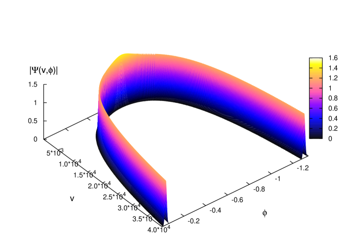
Figure 3: The absolute value of the wave function obtained by evolving an initial data using the method of $\phi$ evolution. For clarity of visualization, only the values of $|\Psi|$ greater than $10^{-4}$ are shown. Being a physical state, $\Psi$ is symmetric under $v\rightarrow-v$. In this simulation, the parameters were: $\varepsilon=2$, $p_{\phi}^{\star}=5\times 10^{3}$, and $\Delta p_{\phi}/p_{\phi}^{\star}=0.025$.

Figure 4: The expectation values (and dispersions) of $\widehat{|v|_{\phi}}$ are plotted for the wave function in Fig. 3 and compared with expanding and contracting classical trajectories.

Figure 5: Plot of the behavior of relative dispersion $\Delta|v|/|v|$ as function of $\phi$. The upper and lower curves correspond to $\Delta p_{\phi}/p_{\phi}^{\star}=0.025$ and $\Delta p_{\phi}/p_{\phi}^{\star}=0.018$ respectively. As can be seen $\Delta|v|/|v|$ is asymptotically a constant for both expanding and contracting branches.

Figure 6: Plot of the behavior of $\langle\rho_{\phi}\rangle$ (points with error bars) and its absolute dispersion (which for clarity is multiplied by 50 and is shown by solid curve). Value of $p_{\phi}^{\star}=10,000$ and $\Delta p_{\phi}/p_{\phi}^{\star}=0.018$.

V.3 Results

Results of various numerical simulations can be summarized as follows:

1. The states remain sharply peaked throughout the evolution. Their norms are preserved under the ‘$\phi$-evolution’, providing a consistency check on the numerics.

2. The classical trajectory provides a good approximation to the expectation values of Dirac observables when the energy density $\rho$ of the scalar field is small compared to a critical energy density $\rho_{\mathrm{crit}}$. However, when this value is reached, the expectation values cease to be peaked at the classical solution. Instead of following the classical trajectory into the big-bang singularity as in the case of the WDW  dynamics, the LQC state undergoes a quantum bounce. The numerical value of $\rho_{\mathrm{crit}}$ was the same in all simulations, given by $\rho_{\mathrm{crit}}\approx 0.82\rho_{\rm Pl}\equiv 0.82/G^{2}\hbar$. A physical understanding of this phenomenon can be obtained from the modified Friedmann equations which incorporate the leading corrections due to quantum geometry effects (see Appendix B.1). These effective equations also provide an analytical expression $\rho_{\mathrm{crit}}=3/(16\pi^{2}\gamma^{3}G^{2}\hbar)$ of the critical density whose numerical value agrees with that found in the simulations of the exact LQC dynamics.

3. On further backward evolution $\rho$ decreases. When it becomes small compared to $\rho_{\mathrm{crit}}$, the state again becomes sharply peaked on a classical solution which has the same value of $\langle\hat{p}_{\phi}\rangle$, but which is contracting in the future. Thus, the quantum geometry effects lead to a resolution of the big bang singularity. Furthermore, the state becomes semi-classical also in the distant past, and the pre and post big-bang branches are joined by a ‘quantum bridge’ by the deterministic evolution of LQC. So long as the initial state at late times is chosen to be semi-classical, this scenario, including the value of $\rho_{\mathrm{crit}}$, is robust. An example of the result of numerical simulation is shown in Fig. 3. The comparison between the classical trajectories and quantum evolution is presented in Fig. 4.

4. In order to better understand the behavior of energy density during quantum evolution we independently analyzed the evolution of expectation values of the energy density operator, defined as $\hat{\rho}_{\phi}=\widehat{p_{\phi}^{2}/2\,p^{3}|_{\phi}}$. Results were consistent with those reported above. We found that in all quantum solutions $\langle\hat{\rho}_{\phi}\rangle$ is bounded above by $\rho_{\mathrm{crit}}\approx 0.82\rho_{\mathrm{Pl}}$. An example of the behavior of the expectation values of $\hat{\rho}_{\phi}$ is presented in Fig. 6.

5. In the regime where quantum gravity modifications to the classical dynamics are negligible, the relative dispersions of Dirac observables were found to remain constant and equal on both sides of the bounce point (see Fig. 5). Thus both semiclassical branches, before and after the bounce, are equally coherent. Close to the bounce point the value of relative dispersion of $\widehat{|v|_{\phi}}$ decreases reaching minimal value exactly at the bounce point. However, this decrease does not imply increased coherence in the large density region. Indeed using the property that states remain sharply peaked, we can find $\Delta\phi$ from $\Delta v/v$ and estimate the uncertainty product $\Delta\phi\Delta p_{\phi}$. While the product remains roughly constant before and after the bounce, it has a small increase near the bounce point.

   Behavior of the dispersion $\Delta\rho_{\phi}$ is shown in Fig. 6. Its value grows in the classical regime in the expanding phase but becomes very small near the bounce point. After the bounce, dispersion again increases, before decreasing in the classical contracting phase. This peculiar variation in $\Delta\rho_{\phi}$ near the quantum bounce can be qualitatively understood using effective theory discussed in Appendix B. It has its origin in the phenomena of super-inflation — i.e. the phase in which $\dot{H}>0$ where $H\equiv\dot{a}/a$ is the Hubble rate— which occurs in the regime $\rho_{\mathrm{crit}}>\rho>\rho_{\mathrm{crit}}/2$ singh:2006a . However, since some of the assumptions that underlie the current derivation of the effective equations are generally violated in the Planck regime, this ‘unreasonable efficacy’ of the effective equations remains somewhat mysterious.

VI Discussion

This is the second in a series of detailed papers whose goal is to develop a comprehensive LQG framework to systematically investigate the physics of the Planck regime near the big bang. In aps2 we analyzed the homogeneous isotropic model with a massless scalar field by introducing several new techniques to construct the physical sector of the theory. We established that, thanks to the quantum geometry effects which distinguish LQC from the WDW  theory, in the backward evolution of states which are semi-classical at late times, the big bang is replaced by a quantum bounce. That investigation was based on the quantum Hamiltonian constraint that has been used in the LQC literature for the last three years. We were able to analyze the physical sector of the theory in detail and firmly establish that, although the quantum evolution dictated by that constraint has several desirable features, it also has a serious flaw: quantum effects can dominate and significantly modify classical predictions even when the matter density (and curvatures) are low aps2 ; dh2 . In this paper we showed that a physically motivated modification of the quantum Hamiltonian constraint overcomes this weakness while preserving the attractive features of the older evolution. Indeed, a key strength of this work is that several features of the present simulations are qualitatively similar to those of aps2 . Finally, in both works, detailed numerical analysis of dynamics was restricted to those quantum states which are semi-classical at late times. Within the model, these states best represent our physical universe and our discussion of the quantum bounce refers only to these states, although evolution is well defined and unitary on the full physical Hilbert space.

We deliberately followed the same organization as aps2 to bring out the (similarities and) differences between the two quantum evolutions. Physically the differences are critically important but mathematically they are rather subtle. This is just as one would expect of an improvement that cures a significant limitation while retaining the strengths of the older method. In Appendix A we outline the inclusion of the cosmological constant. Again, while the previous quantum evolution shows certain departures from the classical theory even when the space-time curvature is low dh2 , the quantum evolution generated by the new Hamiltonian constraint is free of this drawback. Now the departures occur only in the deep Planck regime near the big bang (or the big crunch) and lead to a replacement of the classical singularity by a quantum bounce.

Models discussed so far are too simple to be physically realistic. However, the methods introduced are rather general. In particular, as indicated at the end of section II.1, the ‘$\bar{\mu}$-strategy’ incorporates certain key features of full LQG. Hence, results obtained in this paper provide concrete indications of how quantum geometry can lead to subtle yet important departures from the classical theory by making gravity repulsive in the deep Planck regime. Glimpses of new physics that may emerge were presented in the last section of aps2 . We direct the reader to that paper also for a detailed discussion of numerical analysis, physical ramifications of results and comparisons with other approaches that also feature emergent time and/or quantum bounce.

Finally, as emphasized in section I, a key limitation of the present work is that the theory is not obtained through a systematic symmetry reduction of full LQG. This is inevitable at present because our understanding of the full quantum dynamics of LQG is still very incomplete. The overall framework is constructed by following strategies developed in full LQG. However, an important difference arose in the introduction of the Hamiltonian constraint operator because our mini-superspace reduction is carried out by gauge fixing and is therefore not diffeomorphism invariant. As a result, in the last step we had to use some physical considerations and borrow the expression of the area gap $\Delta$ from the full theory. The strategy in LQC is to begin with simple models and work one’s way up by incorporating the lessons learned along the way. Improved dynamics discussed in this paper is an interesting example of such lessons. Considerable work is now in progress, also by several others, to extend the present analysis to more complicated models that will include anisotropies as well as inhomogeneities.

Acknowledgments: We would like to thank Martin Bojowald, Frank Herrmann and especially Kevin Vandersloot for discussions. This work was supported in part by the NSF grants PHY-0354932 and PHY-0456913, the Alexander von Humboldt Foundation, the Krammers Chair program of the University of Utrecht and the Eberly research funds of Penn State.

Appendix A Non-zero cosmological constant

In this appendix we will investigate the dynamics of the universe with a massless scalar field and a cosmological constant $\Lambda$. Our goal is only to test whether the quantum bounce scenario is robust and if the $\bar{\mu}$-evolution is free of the undesirable features of the $\mu_{o}$-evolution, such as departures from the classical theory at low values of total energy densities dh2 . Therefore the numerical simulations are not as refined as in the main body of the paper. A more systematic and detailed analysis will appear elsewhere.

A negative $\Lambda$ leads to a classical recollapse of the universe when total energy density, including the ‘vacuum energy density’ due to $\Lambda$, vanishes. If a quantum bounce exists in this model then it can lead to a cyclic model of the universe. A positive $\Lambda$ is favored by current observations. For completeness we will discuss both the cases and ask whether general features of the $\Lambda=0$ analysis persist.

The classical Hamiltonian constraint is of the form

$$C_{\Lambda}\ =\ -\frac{6}{\gamma^{2}}c^{2}\sqrt{p}+2\,\Lambda\,|p|^{\frac{3}{2}}+8\pi G|p|^{-\frac{3}{2}}p_{\phi}^{2}\ .$$ (79)

From Hamilton’s equations it is easy to see that the momentum $p_{\phi}$ is again a constant of motion and the scalar field $\phi$ is a monotonic function of time. Hence it is well suited to play the role of emergent time in the quantum theory.

The quantization procedure and the construction of the physical Hilbert space (and observables) for the case $\Lambda\neq 0$ is completely analogous to that in the model with $\Lambda=0$. The quantum Hamiltonian constraint it gives is similar in its form to (53)

$$\partial_{\phi}^{2}\Psi(v,\phi)\ =\ -\Theta_{\Lambda}\Psi(v,\phi)\ :=\ -\left[\Theta-\frac{16\pi^{2}\gamma^{3}{\ell}_{\rm Pl}^{4}}{27K\hbar}[B(v)]^{-1}\Lambda v\right]\Psi(v,\phi)\ ,$$ (80)

where $\Theta_{\Lambda}$ is a self-adjoint operator and $K$ is a constant defined in (17). For $\Lambda>0$ it fails to be positive definite on $\mathcal{H}_{\text{kin}}$. However, since the operator $\partial_{\phi}^{2}$ on the left side of (80) is negative definite, only the projection of $\Theta_{\Lambda}$ on its positive eigenspace is relevant for solutions to the constraint. We can therefore repeat the procedure of section IV.2, decompose the solutions into positive and negative frequency parts, and construct the physical inner product and observables. The expectation values of $\widehat{|v|_{\phi}}$, $\widehat{p_{\phi}}$ and their dispersions at an instant $\phi$ are again given by (77) and (78) respectively, where as the norm of the wave function can be calculated via (64).

The next step is to construct states which are sharply peaked at late times and compare the behavior of the expectation values of observables with classical trajectories. The particular properties of the model differ for $\Lambda<0$ and $\Lambda>0$. Therefore they have to be handled with different methods and we do so separately in sections A.1 ($\Lambda<0$) and A.2 ($\Lambda>0$).

A.1 Negative Cosmological Constant

The classical equations of motion imply that $v(\phi)$ satisfies the following differential equation:

$$\left(\frac{\partial_{\phi}v}{v}\right)^{2}\ =\ 12\pi G+\frac{(4\pi\gamma)^{3}}{(3K)^{2}}v^{2}\frac{\Lambda}{p^{2}_{\phi}}\ .$$ (81)

When the cosmological constant is negative the solution to this equation takes the form

$$v(\phi)\ =\ \sqrt{12\pi G}\frac{3K}{(4\pi\gamma{\ell}_{\rm Pl}^{2})^{3/2}}\frac{p_{\phi}}{\sqrt{|\Lambda|}}|\cosh(\sqrt{12\pi G}(\phi-\phi_{o}))^{-1}|\ .$$ (82)

Thus, the universe originates at the big bang singularity (for $\phi=-\infty$), expands until the recollapse point (at $\phi=\phi_{o}$) where the total energy density (due to the scalar field and the cosmological constant) drops to zero and then contracts, reaching the big crunch singularity at $\phi=+\infty$.

To determine the quantum evolution we apply the method specified in section V.2, that is:

1. We first choose on the $v$ axis the domain $\mathcal{L}_{\varepsilon}\cap[-v_{b},v_{b}]$, where $\mathcal{L}_{\varepsilon}$ is a lattice defined in section IV.1 for some $\varepsilon\neq 0$, and $v_{b}\gg 1$.

2. Next, we specify the initial data, $\Psi(v,\phi_{o})$, $\partial_{\phi}\Psi(v,\phi)|_{\phi_{o}}$, peaked at a phase space point representing an expanding, large classical universe.

3. We evolve this data backward, solving (80) numerically as in section V.2.

4. Finally we calculate the expectation values and their dispersions using (77) and (78)

Figure 7: The expectation values (and dispersions) of $\widehat{|v|_{\phi}}$ for the model with negative cosmological constant are compared with classical trajectories. In this simulation, the parameters were: $\varepsilon=2$, $p_{\phi}^{\star}=5\times 10^{3}$, and $\Lambda=-3.6\times 10^{-3}$, $\Delta p_{\phi}/p_{\phi}^{\star}=0.034$.

We specified the initial state by choosing a Gaussian in $(\mu,c)$ peaked at $\mu^{\star}=K^{-\frac{2}{3}}(v^{\star})^{\frac{2}{3}}$ (see (17)) and $c^{\star}(\mu^{\star},p^{\star}_{\phi})$, and its time derivative by using the classical trajectory. (Thus, we follow ‘method I’ of section V.B.2 of aps2 ). As discussed there, while this method is not as optimal as the one used in main body of this paper, it has the advantage that it does not require the knowledge about properties of the eigenfuncions of $\Theta_{\Lambda}$. The exact forms of these initial profiles were the following:

$$\Psi(v,\phi)|_{\phi_{o}} =|v|^{\frac{1}{2}}e^{-\frac{(\mu(v)-\mu^{\star})^{2}}{2\sigma^{2}}}e^{-\frac{i}{2}(\mu(v)-\mu^{\star})c^{\star}}$$ (83a)

$$\partial_{\phi}\Psi(v,\phi)|_{\phi_{o}} =\ \Psi(v,\phi_{o})\frac{\gamma\beta^{2}}{2p_{\phi}}\left[\frac{i\mu(v)}{3}\left(-\Lambda{\mu^{*}}^{2}+\frac{8\pi Gp_{\phi}^{2}}{\beta^{3}\mu^{*}}\right)+i{\mu^{*}}^{3}\Lambda+\frac{4(\mu(v)-{\mu^{*}}){\mu^{*}}^{2}c^{*}}{\beta\gamma^{2}\sigma^{2}}\right]\ .$$ (83b)

where $\beta:=4\pi\gamma{\ell}_{\rm Pl}^{2}/3$.

Because the domain of integration in numerical simulations is compact in $v$, we have to provide the boundary conditions. Unlike for $\Lambda=0$ however the size of classical universe is bounded by a maximum value $v_{\rm max}$. Therefore, it suffices to choose $v_{b}$ such that the classical recollapse point is well within the domain and set the ‘mirror boundary conditions’: $\Psi=\partial_{\phi}\Psi=0$. In numerical simulations $v_{b}$ was chosen to satisfy the inequality $v_{b}\geq 1.2\,v_{\rm max}$ to make sure that the recollapse occurs due to dynamics and is not an artifact of the boundary conditions.

An example of the result of simulation is presented in fig. 7. The state remains sharply peaked throughout the evolution. The expectation values follow classical trajectory corresponding to the expansion phase till the total energy density

$$\rho_{\text{tot}}=\rho_{\phi}+\rho_{\Lambda},\quad{\rm where}\quad\rho_{\Lambda}:=(8\pi G)^{-1}\Lambda\,,$$ (84)

becomes comparable to $\rho_{\mathrm{crit}}$. At $\rho_{\text{tot}}=\rho_{\mathrm{crit}}$ the universe bounces due to repulsive effects of quantum geometry, and follows contracting phase of classical trajectory. The agreement with classical trajectory remains good through the classical recollapse and expansion phase preceding it, until the energy density becomes large again. Then again a bounce is observed. In effect the evolution is periodic: each ‘cycle’ of classical evolution is connected through quantum bridge with previous/next cycle. Both the Big Bang and Big Crunch singularities are resolved and replaced by quantum bounces. The behavior of fluctuations of Dirac observables is also periodic in the sense that the spread at a given point of the trajectory and after full cycle are the same. Thus, in the fully quantum evolution of LQC, semi-classical states do not loose coherence in evolution from one cycle to another.

A.2 Positive Cosmological Constant

In the case when cosmological constant is positive, classical trajectories, i.e., solutions to (81), take the form

$$v(\phi)\ =\ \sqrt{12\pi G}\frac{3K}{(4\pi\gamma{\ell}_{\rm Pl}^{2})^{3/2}}\frac{p_{\phi}}{\sqrt{|\Lambda|}}|\sinh(\sqrt{12\pi G}(\phi-\phi_{o}))^{-1}|\ .$$ (85)

As for $\Lambda=0$ we have then two types of trajectories. In one the universe starts from a big bang singularity, expands and reaches infinite value of $v$ for finite $\phi=\phi_{o}$. In the other the universe contracts from the infinite volume state (at a finite $\phi=\phi_{o}$) and reaches the big crunch singularity.

The equation (81) implies in particular that in the region where energy density of scalar field is small with respect to vacuum energy density $\rho_{\Lambda}$, the speed $\partial_{\phi}v$ of a wave packet following classical trajectory is proportional to $v^{2}$. This feature, and the fact that to specify proper boundary conditions for evolution in $\phi$ we need to know an explicit form of the square root of the Wheeler-DeWitt limit of the positive part of $\Theta_{\Lambda}$, makes the application of the evolution method numerically difficult. Therefore for the construction of semiclassical states we used the method of direct evaluation of the integral representation of $\Psi(v,\phi)$ specified in section V.1. Thus,

1. We first calculate the symmetric eigenfunctions $e_{k}^{s}(v)$ of the $|\Theta_{\Lambda}|$ operator.

2. Next, we construct the Gaussian state peaked at some $k^{\star}$ and with spread $\sigma$ (see Eq. (70)).

3. Finally, we evaluate the integral (70) using fast Fourier transform and calculate the expectation values.

The exact application of this method requires the normalization of $e^{s}_{k}(v)$ with respect to the inner product given by (64). However, our goal here is only to test robustness of the quantum bounce in presence of a cosmological constant. Therefore, we will not construct semi-classical states which minimize uncertainties but work just with states which are reasonably sharply peaked. Then, it is enough to use for basis eigenfunctions $e^{\prime}{}^{s}_{k}(v):=C(k)e^{s}_{k}(v)$ where $C(k)$ changes slowly with $k$, remaining approximately constant within interval $[k^{\star}-3\sigma,k^{\star}+3\sigma]$. To construct such functions we first observe that, for large $v$, $e^{s}_{k}(v)$ show oscillatory behavior and the absolute values of their extremas decrease as $|v|$ increases and set the ‘normalization’ by requiring equality of maximas closest to the large $v^{\star}$ chosen initially.

An example of the result of simulation is presented in figure 8. The state indeed is sharply peaked. As in the case $\Lambda=0$, the expectation values of $\widehat{|v|_{\phi}}$ again reproduce the picture of two semiclassical regions, one contracting and the other expanding, connected by a quantum bounce. The total energy density (defined via (84)) at the bounce point equals $\rho_{\mathrm{crit}}$. Unlike in the $\Lambda=0$ case however the universe shrinks from $v=\infty$, bounces and again re-expands to $v=\infty$, all within a compact interval of $\phi$.

Figure 8: The expectation values (and dispersions) of $\widehat{|v|_{\phi}}$ for the model with positive cosmological constant are compared with classical trajectories. In this simulation, the parameters were: $\varepsilon=2$, $p_{\phi}^{\star}=1.6\times 10^{3}$, and $\Lambda=4.1\times 10^{-2}$. Horizontal dashed lines denote asymptotic values of $\phi$ for which $v\to\infty$.

To summarize, in both cases ($\Lambda>0$ and $\Lambda<0$):

1. Classical singularity is replaced by a quantum bounce, which occurs when $\rho_{\text{tot}}=\rho_{\phi}+\rho_{\Lambda}=\rho_{\mathrm{crit}}$. The critical value of energy density was found numerically to be equal to $0.82\rho_{\mathrm{Pl}}$. Thus, the value of $\rho_{\mathrm{crit}}$ is independent of the value of cosmological constant. Analysis of the modified Friedmann equation on the lines of Appendix B yields the same expression, $\rho_{\mathrm{crit}}=\sqrt{3}/(16\pi^{2}\gamma^{3}G^{2}\hbar)$, of the critical density.

2. In the dynamics dictated by the Hamiltonian constraint used so far in literature, a deviation from the classical behavior resulting in a recollapse occurs at low energy density scales, when cosmological constant dominates dh2 . The improved dynamics presented in this work is free of this physically undesirable feature. More generally, the new dynamics reproduces the standard Friedmann dynamics when $\rho\ll\rho_{\mathrm{crit}}$.

Appendix B Some conceptual issues

B.1 Effective dynamics

An effective description of quantum dynamics can be obtained by applying geometric methods to quantum mechanics, where the Hilbert space is treated as an infinite dimensional phase space which has a structure of a fiber bundle (see, e.g., as ; jw ). The base space of this bundle is the classical phase space and fibers are the states with same expectation values of the operators for the corresponding canonically conjugate phase space variables. Using coherent states we can attempt to find horizontal sections which are preserved under the quantum evolution up to some desired accuracy, and can thus obtain an effective Hamiltonian which incorporates the leading quantum corrections to the classical dynamics.

Let us consider the $\Lambda=0$ case as in the main body of the paper. Then, for LQC, this procedure leads to an effective Hamiltonian with leading order terms as vt :

$${\cal H}_{\mathrm{eff}}=\frac{C_{\rm eff}}{16\pi G}=-\frac{3}{8\pi G\gamma^{2}\bar{\mu}^{2}}|p|^{\frac{1}{2}}\,\sin^{2}(\bar{\mu}c)+\frac{1}{2}\,B(p)\,{p_{\phi}^{2}}~{}.$$ (86)

Here $B(p)$ denotes the eigenvalue of $\widehat{1/|p|^{3/2}}$ operator given by (31). Modifications to the dynamics due to behavior of $B(p)$ become significant for $|v|\sim 1$. For $|v|\gg 1$, $B(p)$ quickly approaches the classical value $|p|^{-3/2}$, proportional to $1/|v|$ and the rate of approach is given by

$$B(p)=\left(\frac{6}{8\pi\gamma{\ell}_{\rm Pl}^{2}}\right)^{3/2}\,\frac{K}{|v|}\left(1+\frac{5}{9}\,\frac{1}{|v|^{2}}+O\left(\frac{1}{|v|^{4}}\right)\right)~{}.$$ (87)

Neglecting the higher order quantum corrections to $B(p)$ we can obtain the Hamilton’s equation for $v$ and $\phi$:

$$\dot{v}=\{v,\,{\cal H}_{\mathrm{eff}}\}=-\frac{8\pi\gamma G}{3}\,\frac{\partial{\cal H}_{\mathrm{eff}}}{\partial c}=\frac{2|v|^{1/3}}{\gamma\bar{\mu}K}\,\left(\frac{8\pi\gamma{\ell}_{\rm Pl}^{2}}{6}\right)^{1/2}\,\sin(\bar{\mu}c)\,\cos(\bar{\mu}c)~{}.$$ (88)

and

$$\dot{\phi}=\{\phi,{\cal H}_{\mathrm{eff}}\}=\left(\frac{8\pi\gamma{\ell}_{\rm Pl}^{2}}{6}\right)^{-3/2}\,K\,\frac{p_{\phi}}{|v|}\,.$$ (89)

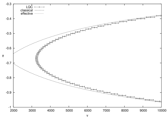
Figure 9: A comparison of the quantum dynamics represented by the expectation values and dispersions of $\widehat{|v|_{\phi}}$ (points with error bars), the effective dynamics (dotted curve) and the classical dynamics (dashed curve) is presented near the bounce point. The effective dynamics provides a good approximation to the underlying quantum theory. The values of parameters were $p_{\phi}=10000$ and $\varepsilon=2$.

The modified Friedmann equation can be obtained from the vanishing of the Hamiltonian constraint (86):

$$\sin^{2}(\bar{\mu}c)=\frac{8\pi\gamma^{2}\bar{\mu}^{2}G}{6\,|p|^{2}}\,p_{\phi}^{2}\,,$$ (90)

and using Eq.(88). It turns out to be

$$H^{2}\equiv\frac{\dot{v}^{2}}{9v^{2}}=\frac{8\pi G}{3}\,\rho\left(1-\frac{\rho}{\rho_{\mathrm{crit}}}\right),\quad{\rm where}\quad\rho_{\mathrm{crit}}=\frac{\sqrt{3}}{16\pi^{2}\gamma^{3}G^{2}\hbar}~{},$$ (91)

with $\rho=p_{\phi}^{2}/2|p|^{3}$. Quantum geometry effects thus lead to $\rho^{2}$ modification of the Friedmann equation at the scales when $\rho$ becomes comparable to $\rho_{\mathrm{crit}}$. The Hubble parameter vanishes when energy density becomes equal to the critical value $\rho_{\mathrm{crit}}$ and the universe bounces from the expanding (contracting) branch to the contracting (expanding) branch. Further, $\rho/\rho_{\mathrm{crit}}$ term becomes negligible for $\rho\ll\rho_{\mathrm{crit}}$ and Eq. (91) reduces to the standard Friedmann equation; there are no departures from classical general relativity in the low curvature regime. Detailed phenomenological investigations of the effective theory obtained from the improved quantum constraint confirm that unnatural effects of the old quantization are cured in the improved quantization imp_pheno .

To compare effective dynamics with the exact quantum evolution in Sec. V.2, it is useful to combine (88) and (89) to obtain:

$$\frac{dv}{d\phi}=\sqrt{12\pi G}\,\left(1-\frac{\rho}{\rho_{\mathrm{crit}}}\right)^{1/2}\,v~{}.$$ (92)

Trajectories obtained from this equation are plotted in Fig.9 and compared with the expectation values of $\widehat{|v|_{\phi}}$ and the classical dynamics. As can be seen, the effective dynamics provides an excellent approximation to the underlying quantum dynamics.

Remark: The modified field equations (91) and (92) can be interpreted as saying that the effective Newton’s constant is given by $G_{\rm eff}=G(1-{\rho}/{\rho_{\mathrm{crit}}})$, where $G$ is the low energy Newton’s constant and $\rho_{\mathrm{crit}}\approx 0.82\rho_{\rm Pl}$. Now, the renormalization group analysis based on Euclidean quantum gravity mr strongly suggests the existence of a non-trivial fixed point at which the theory becomes asymptotically free. The behavior of $G_{\rm eff}$ in LQC is in qualitative agreement with that picture.

B.2 Subtleties associated with $k=0$ cosmologies

To write the space-time metric in the standard FRW form, $g_{ab}=-\nabla_{a}t\nabla_{b}t+a^{2}(t)q^{o}_{ab}$, one needs a fiducial, Riemannian 3-metric $q^{o}_{ab}$ of constant curvature $k$. Clearly, under a rescaling $q^{o}_{ab}\rightarrow\alpha^{2}q^{o}_{ab}$, the scale factor $a(t)$ scales as $a(t)\rightarrow\alpha^{-1}a(t)$. As is well-known, while this rescaling freedom can be eliminated in the $k=\pm 1$ cases by requiring that $q^{o}_{ab}$ be the unit 3-sphere or unit 3-hyperboloid metric, in the $k=0$ case there is no natural way to select a unique $q^{o}_{ab}$ whence the scale factor $a(t)$ by itself does not have a direct physical meaning. This feature introduces certain subtleties in the Hamiltonian framework in the $k=0$ case. The purpose of this appendix is to summarize them and correct certain misconceptions that have permeated in some of the LQG literature.

The Hamiltonian framework has more information than that contained in the equations of motion. In particular the symplectic structure can be regarded as the imprint left by the quantum theory on the classical framework. To define the correct symplectic structure and Hamiltonian in the non-compact, homogeneous context, one has to introduce a fiducial cell $\mathcal{V}$ and restrict all integrations to it. In the $k=-1$ case, one can fix $\mathcal{V}$ to have unit volume with respect to the unit hyperboloid metric. In the $k=0$ case, such a simple prescription is not available. However, once $\mathcal{V}$ is chosen, its presence can be used to make the canonical variables, the symplectic structure and the Hamiltonian insensitive to the choice of the fiducial metric $q^{o}_{ab}$ abl . This was the procedure followed in aps2 as well as in the present paper. For each choice of $\mathcal{V}$ we obtain a physical theory. In that theory, one can make well-defined predictions. However, since in the $k=0$ case there is no physical procedure to fix the fiducial cell, we now have a new ‘gauge freedom’ $\mathcal{V}\rightarrow\lambda^{3}\mathcal{V}$. Under this rescaling the theory changes. Only those quantities which are insensitive to this rescaling can be regarded as physical.

Recall that in the quantum theory $\hat{V}\equiv|\hat{p}|^{3/2}$ is the volume operator associated with the fiducial cell $\mathcal{V}$. Thus, $|\mu\rangle$ (respectively $|v\rangle$) is an eigenstate of quantum geometry in which the volume of $\mathcal{V}$ is $|p|^{3/2}\equiv(8\pi\gamma/6)^{3/2}\,|\mu|^{3/2}\,{\ell}_{\rm Pl}^{3}$ (respectively $(8\pi\gamma/6)^{3/2}\,(3\sqrt{3\sqrt{3}}/2\sqrt{2})\,v\,{\ell}_{\rm Pl}^{3}$). Now, in the quantum theory based on the cell $\mathcal{V}$, $|1/p|^{3/2}$ ceases to be a good approximation to the eigenvalues of the inverse volume operator $\widehat{1/V}$ for $\mu<\mu_{\star}$, for a well-defined real number $\mu_{\star}$ (which makes no reference to the size fiducial cell $\mathcal{V}$). Therefore one sometimes finds statements in the LQC literature to the effect that the quantum geometry effects become important when $\mu<\mu_{\star}$. However, physically this would mean that the quantum geometry effects become important when the physical volume of $\mathcal{V}$ is less that $|p_{\star}|^{3/2}$. Clearly, since the fiducial cell cannot be fixed unambiguously in the $k=0$ case, unlike in the $k=\pm 1$ cases, this tempting suggestion has no invariant meaning. Put differently, from a space-time perspective, one can begin with a quadruplet $(q_{ab},\phi;\,\dot{q}_{ab},\dot{\phi})$ representing the initial data at late times for an expanding universe, consider a semi-classical quantum state which is sharply peaked about this configuration and ask when, in the backward quantum evolution, there are significant departures from the classical trajectory. The answer to this physical question cannot depend on the choice of the fiducial cell used in the construction of quantum theory. Therefore, in the $k=0$ case, the answer that this happens at $p=p_{\star}$ is not viable. Similarly, in the analysis of the quantum bounce, the value of $p_{\rm crit}$ (or $v_{\rm crit}$) at which the bounce occurs has only mathematical meaning within the theory based on a specific $\mathcal{V}$. From a space-time perspective, this is not surprising: it is well-known that the value of the scale factor at which something specific happens is tied to the choice of fiducial metric and therefore has no invariant meaning.

On the other hand, in the classical theory the matter density $\rho$ has direct physical meaning also in the $k=0$ case from both the space-time and the phase space perspectives. In the space-time perspective, it is given by $\rho=(\dot{\phi})^{2}/2$ and makes no reference to the fiducial metric. From the phase space perspective it is given by $\rho=p_{\phi}^{2}/2|p|^{3}$ and is insensitive to the choice of $\mathcal{V}$ because under the rescaling $\mathcal{V}\rightarrow\lambda^{3}\mathcal{V}$,  $p_{\phi}\rightarrow\lambda^{3}p_{\phi}$ and $|p|\rightarrow\lambda^{2}|p|$. Therefore it is physically meaningful to ask if there is a critical value of density $\rho_{\mathrm{crit}}$ at which the classical theory becomes inadequate. Numerical simulations show that the LQC dynamics used in the literature yields $\rho_{\mathrm{crit}}=k|p_{\rm crit}|=k^{\prime}/(p_{\phi})$, where $k$ and $k^{\prime}$ are constants that do not depend on $\mathcal{V}$ and $p_{\rm crit}$ refers to the value of $p$ of at the bounce point. The physical meaning of $|p|$ and $p_{\phi}\equiv\dot{\phi}\,|p|^{3/2}$ depends on the choice of $\mathcal{V}$. Since $\rho$ itself is gauge invariant, i.e., is independent of the choice of the fiducial metric $q^{o}_{ab}$ or the fiducial cell $\mathcal{V}$, there is a conceptual mismatch. By contrast, the quantum dynamics presented in this paper leads to $\rho_{\mathrm{crit}}\approx 0.82\rho_{\rm Pl}$ for any state which is semi-classical at late times; in particular, $\rho_{\mathrm{crit}}$ makes no reference to the fiducial cell $\mathcal{V}$.

To summarize, whether one works with geometrodynamics or path integrals or LQG, the introduction of a fiducial cell $\mathcal{V}$ is essential in quantization of spatially non-compact homogeneous models. $\mathcal{V}$ can be used to remove the reference to the fiducial metric $q^{o}_{ab}$ from the theory. However, its presence introduces a new ‘gauge’ freedom and one has to exercise due care in the physical interpretation of the theory. If we have two theories, the first based on a fiducial cell $\mathcal{V}_{1}$ and the second on $\mathcal{V}_{2}=\lambda^{3}\mathcal{V}_{1}$, the state $|\mu\rangle$ (or $|v\rangle$) of the first theory is physically the same as the state $|\lambda^{2}\mu\rangle$ (respectively $|\lambda^{3}v\rangle$) of the second theory. Using this equivalence, one has to ensure that the final physical results are independent of the choice of the initial fiducial cell.

We will conclude with the discussion of a subtlety. Fix a fiducial cell $\mathcal{V}$ and consider the resulting quantum theory. Then, for $v<v_{\star}$ the inverse volume corrections become important and the functional form of $\rho(p_{\phi},p)$ is significantly different from the classical relation $\rho=p_{\phi}^{2}/2p^{3}$. Therefore, if a trajectory were to enter this region, the quantum corrected $\rho$ along it does not increase and may never reach the critical value $\rho_{\mathrm{crit}}$. Then the argument for a quantum bounce would break down. But a detailed analytical and numerical examination shows that this could happen only if the assumption $p_{\phi}\gg\hbar$ (in c=G=1 units) is violated. In a state which is peaked at such a small $p_{\phi}$, the uncertainty in the Dirac observables becomes comparable to the values of the observables themselves, whence the state can not be regarded as semi-classical. Such a state falls outside both the detailed quantum evolution studied in the main body of the paper and the realm of effective equations developed in Appendix B.1.

References

- (1) A. Ashtekar, T. Pawlowski and P. Singh, Quantum nature of the big bang: An analytical and numerical investigation I, Phys. Rev. D, at press, arXiv:gr-qc/0604013.
- (2) A. Ashtekar, T. Pawlowski and P. Singh, Quantum nature of the big bang, Phys. Rev. Lett. 96, 141301 (2006), arXiv:gr-qc/0602086.
- (3) M. Bojowald, Absence of singularity in loop quantum cosmology, Phys. Rev. Lett. 86, 5227-5230 (2001), arXiv:gr-qc/0102069, Isotropic loop quantum cosmology, Class. Quantum. Grav. 19, 2717-2741 (2002), arXiv:gr-qc/0202077.
- (4) A. Ashtekar, M. Bojowald, J. Lewandowski, Mathematical structure of loop quantum cosmology, Adv. Theo. Math. Phys. 7, 233-268 (2003), gr-qc/0304074.
- (5) M. Bojowald, Loop quantum cosmology, Liv. Rev. Rel. 8, 11 (2005), arXiv:gr-qc/0601085.
-
(6)
K. Banerjee, G. Date, Discreteness corrections to the
effective Hamiltonian of isotropic loop quantum cosmology, Class.
Quant. Grav. 22 (2005) 2017, arXiv:gr-qc/0501102;
K. Noui, A. Perez, K. Vandersloot, On the Physical Hilbert Space of Loop Quantum Cosmology, Phys. Rev. D 71 (2005) 044025, gr-qc/0411039. - (7) A. Ashtekar and J. Lewandowski, Background independent quantum gravity: A status report, Class. Quant. Grav. 21, R53-R152 (2004), arXiv:gr-qc/0404018.
- (8) C. Rovelli Quantum Gravity, (CUP, Cambridge, 2004).
- (9) T. Thiemann, Introduction to Modern Canonical Quantum General Relativity (CUP, Cambridge, at press).
- (10) A. Ashtekar, J. Lewandowski, D. Marolf, J. Mourão and T. Thiemann, Quantization of diffeomorphism invariant theories of connections with local degrees of freedom Jour. Math. Phys. 36 6456–6493 (1995), arXiv:gr-qc/9504018.
- (11) C. Rovelli and L. Smolin Discreteness of area and volume in quantum gravity Nucl. Phys. B442 593–622 (1995); Erratum: Nucl. Phys. B456 753, (1996) gr-qc/9411005.
- (12) A. Ashtekar and J. Lewandowski, Quantum theory of geometry I: Area operators, Class. Quant. Grav. 14 A55–A81 (1997), arXiv:gr-qc/9602046.
- (13) A. Ashtekar, Geometry, gravity and the quantum, in the Proceedings of the Einstein Century Conference, edited by J-M Alimi et al, (AIP, New York, in Press), arXiv:gr-qc/0605011.
- (14) A. Ashtekar, S. Fairhurst and J. Willis, Quantum gravity, shadow states, and quantum mechanics, Class. Quantum Grav. 20, 1031-1062 (2003), arXiv:gr-qc/0207106.
-
(15)
Thiemann, T. Anomaly-free formulation of
non-perturbative, four-dimensional Lorentzian quantum gravity,
Phys. Lett. B380, 257–264 (1998),
gr-qc/9606088,
Quantum spin dynamics (QSD), Class. Quant. Grav. 15 839–873 (1998), gr-qc/9606089,
QSD V : Quantum gravity as the natural regulator of matter quantum field theories, Class. Quant. Grav. 15, 1281–1314 (1998), gr-qc/9705019. - (16) M. Bojowald, Personal Communication (2006).
- (17) N. M. J Woodhouse, Geometric Quantization, (Oxford UP, Oxford, 1997).
- (18) M. Bojowald, Quantization ambiguities in isotropic quantum geometry, Class. Quant. Grav. 19, 5113 (2002), gr-qc/0206053.
-
(19)
K. Vandersloot, On the Hamiltonian constraint of loop
quantum cosmology, Phys. Rev. D71 103506 (2005),
gr-qc/0502082;
Ph.D. Dissertation, submitted to The Pennsylvania State University (2006). - (20) A. Perez, On the regularization ambiguities in loop quantum gravity, Phys.Rev. D 73 (2006) 044007, arXiv:gr-qc/0509118.
- (21) W. Kaminski, personal communication to AA (November 2005).
- (22) A. Ashtekar and R. Geroch, Quantum theory of gravitation, Rep. Prog. Phys. 37, 1211-1256 (1974).
- (23) C. Kiefer, Wave packets in minisuperspace, Phys. Rev. Rev. D38, 1761-1772 (1988).
- (24) A. Ashtekar, Lectures on non-perturbative canonical gravity, Notes prepared in collaboration with R. S. Tate (World Scientific, Singapore, 1991), Chapter 10.
- (25) A. Ashtekar and R. S. Tate, An algebraic extension of Dirac quantization: Examples, Jour. Math. Phys. 35 6434–6470 (1994).
-
(26)
D. Marolf, Refined algebraic quantization:
Systems with a single constraint arXives:gr-qc/9508015;
Quantum observables and recollapsing dynamics, Class. Quant. Grav. 12 (1995) 1199-1220 arXiv:gr-qc:9404053
Observables and a Hilbert space for Bianchi IX, Class. Quant. Grav. 12 (1995) 1441-1454 arXiv:gr-qc:9409049
Almost ideal clocks in quantum cosmology: A brief derivation of time, Class. Quant. Grav. 12 (1995) 2469-2486 arXiv:gr-qc:9412016. - (27) J. B. Hartle and D. Marolf, Comparing formulations of generalized quantum mechanics for reparametrization-invariant systems, Phys. Rev. D56, 6247-6257 (1997) arXiv:gr-qc:9703021.
- (28) P. Singh, Loop cosmological dynamics and dualities with Randall-Sundrum braneworlds, Phys. Rev. D73 063508 (2006), arXiv:gr-qc/0603043.
- (29) A. Ashtekar and T. Schilling, Geometrical formulation of quantum mechanics, In: On Einstein’s path, A. Harvery, ed (Springer-Verlag, New York, 1998); arXiv:gr-qc/9706069. T. Schilling, Geometry of quantum mechanics, Ph.D. Dissertation, Penn State (1996), http://cgpg.gravity.psu.edu/archives/thesis/index.shtml
- (30) J. Willis, On the low energy ramifications and a mathematical extension of loop quantum gravity, Ph.D. Dissertation, The Pennsylvania State University (2004); A. Ashtekar, M. Bojowald and J. Willis, Corrections to Friedmann equations induced by quantum geometry, IGPG preprint (2004).
- (31) V. Taveras, IGPG preprint (2006).
- (32) P. Singh, K. Vandersloot, G. V. Vereshchagin, Non-Singular Bouncing Universes in Loop Quantum Cosmology, Phys. Rev. D74 043510 (2006); arXiv:gr-qc/0606032.
- (33) M. Reuter and F. Saueressig, From big bang to asymptotic de Sitter: Complete cosmologies in a quantum gravity framework, JCAP 0509, 012 (2005), hep-th/0507167.