Positioning with stationary emitters
in a two-dimensional space-time

Abstract

The basic elements of the relativistic positioning systems in a two-dimensional space-time have been introduced in a previous work [Phys. Rev. D 73, 084017 (2006)] where geodesic positioning systems, constituted by two geodesic emitters, have been considered in a flat space-time. Here, we want to show in what precise senses positioning systems allow to make relativistic gravimetry. For this purpose, we consider stationary positioning systems, constituted by two uniformly accelerated emitters separated by a constant distance, in two different situations: absence of gravitational field (Minkowski plane) and presence of a gravitational mass (Schwarzschild plane). The physical coordinate system constituted by the electromagnetic signals broadcasting the proper time of the emitters are the so called emission coordinates, and we show that, in such emission coordinates, the trajectories of the emitters in both situations, absence and presence of a gravitational field, are identical. The interesting point is that, in spite of this fact, particular additional information on the system or on the user allows not only to distinguish both space-times, but also to complete the dynamical description of emitters and user and even to measure the mass of the gravitational field. The precise information under which these dynamical and gravimetric results may be obtained is carefully pointed out.

I Introduction

A relativistic positioning system is defined by four clocks $\gamma_{i}$ (emitters) in arbitrary motion broadcasting their proper times $\tau^{i}$ in some region of a (four-dimensional) space-time cfm-a ; coll-1 . The future light cones of the points $\gamma_{i}(\tau^{i})$ constitute coordinate hypersurfaces $\tau^{i}=constant$ of a coordinate system for that region. Indeed, at every event of the domain, four of these cones broadcasting the times $\tau^{i}$ intersect, endowing thus the event with the emission coordinates $\{\tau^{i}\}:$ the four proper time signals received by any observer at the event from the four clocks.

As a location system (i.e. as a physical realization of a mathematical coordinate system) coll-1 ; coll-3 , the above positioning system presents interesting qualities and, among them, those of being generic, (gravity-)free and immediate. This fact has been pointed out elsewhere cfm-a ; coll-1 ; coll-2 ; coll-3 and some explicit results have been recently obtained for the generic four-dimensional case coll-pozo-1 ; coll-pozo-2 ; pozo .

A full development of the theory for this generic case requires a hard task and a previous training on simple and particular situations. In cfm-a we have presented a two-dimensional approach to relativistic positioning systems introducing the basic features that define them. We have obtained the explicit relation between emission coordinates and any given null coordinate system wherein the proper time trajectories of the emitters are known. We have also developed in detail the positioning system defined in flat space-time by geodesic emitters. Finally, we have shown that, in arbitrary two-dimensional space-times, the data that a user obtains from the positioning system determine the gravitational field and its gradient along the emitters and user world lines.

This two-dimensional approach has the advantage of allowing the use of precise and explicit diagrams which improve the qualitative comprehension of general four-dimensional positioning systems. Moreover, two-dimensional scenarios admit simple and explicit analytic results. These advantages encourage us in proposing and solving new two-dimensional problems, many of them already suggested in a natural way by the results presented in cfm-a .

In the present work we want to detect the possibility of making relativistic gravimetry or, more generally, the possibility of obtaining the dynamics of the emitters and/or of the user, as well as the detection of the absence or presence of a gravitational field and its measure. This possibility is here examined by means of a (non geodesic) stationary positioning system, that is to say a positioning system whose emitters are uniformly accelerated and the radar distance from each one to the other is constant. Such a stationary positioning system is constructed in two different scenarios: Minkowski and Schwarzschild planes.

In both scenarios, and for any user, the trajectory of the emitters in the grid, i.e. in the plane $\{\tau^{1}\}\times\{\tau^{2}\},$ are two parallel straight lines. At first glance, this fact would seem to indicate the impossibility to extract dynamical or gravimetric information from them, but this appearance is deceptive.

We shall prove that the simple qualitative information that the positioning system is stationary (but with no knowledge of the acceleration and mutual radar distance of every emitter) and that the space-time is created by a given mass (but with no knowledge of the particular stationary trajectories followed by the emitters) allows to know the actual accelerations of the emitters, their mutual radar distances and the space-time metric in the region between them in emission coordinates $\{\tau^{i}\}.$ Also, the transformations to other standard coordinate systems may be obtained.

The important point for gravimetry is that, in the above context, the data of The Schwarzschild mass may be substituted by that of the acceleration of one of the emitters. Then, besides all the above mentioned results, including the obtaining of the acceleration of the other emitter, the actual The Schwarzschild mass of the corresponding space-time may be also calculated.

These relatively simple two-dimensional results strongly suggests that relativistic positioning systems can be useful in gravimetry at least when parameterized models for the gravitational field may be proposed.

A comment about the presentation of the results. The user is supposed to continuously receive data from the positioning system and have some a priori information about it and/or the space-time. Because of their operational importance, the statements involving exclusively consequences of these two types of knowledge, have been emphasized and numbered.

The work is organized as follows. In Sec. II we summarize the basic concepts and notation about relativistic positioning systems in a two-dimensional space-time. Sections III and IV are devoted to the analysis of stationary positioning systems respectively in Minkowski and in Schwarzschild planes. In sections V and VI we analyze the roles that different user’s data play in obtaining the gravitational field and in recovering the characteristics of the positioning system. Finally, we finish with a short discussion about the present results and comments on prospective work in Sec. VII.

II Summary of previous results

In a two-dimensional space-time, let $\gamma_{1}$ and $\gamma_{2}$ be the world lines of two clocks measuring their proper times $\tau^{1}$ and $\tau^{2}$ respectively. Suppose they broadcast them by means of electromagnetic signals, and that the signals from each one of the world lines reach the other. This system of two clocks (emitters) is called a relativistic positioning system.

A domain $\Omega$ in the region between both emitters constitutes a coordinate domain. Indeed, the past light cone of every event in $\Omega$ cuts the emitter world lines at $\gamma_{1}(\tau^{1})$ and $\gamma_{2}(\tau^{2})$, respectively. Then $(\tau^{1},\tau^{2})$ are the coordinates of the event: the two proper time signals received by any observer at the event from the two clocks. We shall refer to them as the emission coordinates $\{\tau^{1},\tau^{2}\}$ of the system in $\Omega$. Also, by continuity, we shall call emission coordinates of the emitters the pair of proper times formed by the proper time of the clock in question and that received from the other clock. Nevertheless, the signals $\tau^{1}$ and $\tau^{2}$ do not constitute coordinates for the events in the outside region.

The plane $\{\tau^{1}\}\times\{\tau^{2}\}$ ($\tau^{1},\tau^{2}\in\mathbb{R}$) in which the different data of the positioning system can be transcribed is called, as already remembered, the grid of the positioning system. In this grid, the trajectories of the two emitters (which, for the auto-locating positioning systems considered below, can be drawn from the positioning data broadcast by the emitters) define an interior region and two exterior ones. This interior region in the grid is in one-to-one correspondence with the interior region in the space-time, i.e. with the set of events that can be distinguished by the pair of times $(\tau^{1},\tau^{2})$ that reach them. But the exterior regions in the grid are not in one-to-one correspondence with the corresponding exterior regions in the space-time, because these last regions are foliated by null geodesics whose events have all the same values $(\tau^{1},\tau^{2})$ that the emission coordinates of the emitter that borders the region. So, the pairs $(\tau^{1},\tau^{2})$ of the exterior regions in the grid are not emission coordinates: they do not correspond to pairs of signals broadcast by the two emitters. Consequently, for this emission protocol, they do not correspond to points of the two-dimensional space-time (nevertheless, as mathematical extensions, they could be of interest in some situations). The grid origin depends exclusively on the choice of the instant zero of the emitter clocks. This synchronization is not a necessary prior information for positioning and it can be obtained from the system data.

Emission coordinates are null coordinates and thus the space-time metric depends on the sole metric function $m$:

$$ds^{2}=m(\tau^{1},\tau^{2})d\tau^{1}d\tau^{2}$$ (1)

An observer $\gamma,$ traveling throughout an emission coordinate domain $\Omega$ and equipped with a receiver allowing the reading of the received proper times $(\tau^{1},\tau^{2})$ at each point of his trajectory, is called a user of the positioning system.

From now on we will consider auto-locating positioning systems, which are systems in which every emitter clock not only broadcasts its proper time but also the proper time that it receives from the other, i.e. the systems that broadcast the emission coordinates of the emitters. Thus, the physical components of an auto-locating positioning system are cfm-a a spatial segment constituted by two emitters $\gamma_{1}$, $\gamma_{2}$ broadcasting their proper times $\tau^{1},$ $\tau^{2}$ and the proper times $\bar{\tau}^{2}$, $\bar{\tau}^{1}$ that they receive each one from the other, and a user segment constituted by the set of all users traveling in an internal domain $\Omega$ and receiving these four broadcast times $\{\tau^{1},\tau^{2};\bar{\tau}^{1},\bar{\tau}^{2}\}$.

It is worth remarking that any user receiving continuously the emitted times $\{\tau^{1},\tau^{2}\}$ knows his trajectory in the grid. Indeed, from these user positioning data $\{\tau^{1},\tau^{2}\}$ the equation $F$ of the user trajectory may be extracted:

$$\tau^{2}=F(\tau^{1})$$ (2)

On the other hand, any user receiving continuously the emitter positioning data $\{\tau^{1},\tau^{2};\bar{\tau}^{1},\bar{\tau}^{2}\}$ may extract from them not only the equation (2) of his trajectory, but also the equations of the trajectories of the emitters in the grid:

$$\varphi_{1}(\tau^{1})=\bar{\tau}^{2}\,,\qquad\varphi_{2}(\tau^{2})=\bar{\tau}^{1}$$ (3)

Eventually, the positioning system can be endowed with complementary devices. Thus, in order to obtain the dynamic properties of the system, the emitters $\gamma_{1}$, $\gamma_{2}$ could carry accelerometers and broadcast their acceleration $\alpha_{1}$, $\alpha_{2}$, meanwhile the users $\gamma$ could be endowed with receivers able to read, in addition to the emitter positioning data, also the broadcast emitter accelerations $\{\alpha_{1},\alpha_{2}\}$. These new elements allow any user to know the acceleration scalar of the emitters:

$$\alpha_{1}=\alpha_{1}(\tau^{1})\,,\qquad\alpha_{2}=\alpha_{2}(\tau^{2})$$ (4)

In some cases, it can be useful that the users generate their own data, carrying a clock to measure their proper time and/or an accelerometer to measure their proper acceleration $\alpha$. The user’s clock allows any user to know his proper time function $\tau(\tau^{1})$ (or $\tau(\tau^{2})$) and, consequently by using (2), to obtain the proper time parametrization of his trajectory:

$$\gamma\equiv\begin{cases}\ \tau^{1}=\tau^{1}(\tau)\\ \ \tau^{2}=\tau^{2}(\tau)\end{cases}$$ (5)

The user’s accelerometer allows any user to know his proper acceleration scalar:

$$\alpha=\alpha(\tau)$$

Thus, a relativistic positioning system may generate the user data:

$$\{\tau^{1},\tau^{2};\bar{\tau}^{1},\bar{\tau}^{2};\alpha_{1},\alpha_{2};\tau,\alpha\}$$ (6)

The emitter trajectories (3) and the emitter accelerations (4) do not depend on the user that receives them. Thus, among the user data (6) we can distinguish besides the emitter positioning data $\{\tau^{1},\tau^{2};\bar{\tau}^{1},\bar{\tau}^{2}\}$, the emitter dynamical data $\{\alpha_{1},\alpha_{2}\}$, their union or public data $\{\tau^{1},\tau^{2};\bar{\tau}^{1},\bar{\tau}^{2};\alpha_{1},\alpha_{2}\}$ and the user proper data $\{\tau,\alpha\}$.

The purpose of the (relativistic) theory of positioning systems is to develop the techniques necessary to determine the space-time metric as well as the dynamics of emitters and users by means of physical information carried by light signals. But in order to develop it in known space-times, it is useful to connect our emission coordinates to the usual coordinates in which these space-times have been already studied. We finish this section by summarizing the explicit obtaining of the emission coordinates from an arbitrary null coordinate system $\{\texttt{u},\texttt{v}\}$ in a generic two-dimensional space-time cfm-a . Let us assume the proper time history of two emitters to be known in this coordinate system:

$$\gamma_{1}\equiv\begin{cases}\texttt{u}=u_{1}(\tau^{1})\\ \texttt{v}=v_{1}(\tau^{1})\end{cases}\qquad\gamma_{2}\equiv\begin{cases}\texttt{u}=u_{2}(\tau^{2})\\ \texttt{v}=v_{2}(\tau^{2})\end{cases}$$ (7)

We can introduce the proper times as coordinates $\{\tau^{1},\tau^{2}\}$ by defining the transformation to the null system $\{\texttt{u},\texttt{v}\}$ given by:

$$\begin{array}[]{l}\texttt{u}=u_{1}(\tau^{1})\\ \texttt{v}=v_{2}(\tau^{2})\end{array}\qquad\quad\begin{array}[]{l}\tau^{1}=u_{1}^{-1}(\texttt{u})=\tau^{1}(\texttt{u})\\ \tau^{2}=v_{2}^{-1}(\texttt{v})=\tau^{2}(\texttt{v})\end{array}$$ (8)

Thus, relations (8) define emission coordinates in the emission coordinate domains $\Omega$ between both emitters. Note that outside this region of domains the transformation (8) also determines null coordinates, but they are not emission coordinates, i.e. they cannot be constructed by means of broadcast signals cfm-a .

In emission coordinates, the emitter trajectories take the expression:

$$\gamma_{1}\equiv\begin{cases}\tau^{1}=\tau^{1}\\ \tau^{2}=\varphi_{1}(\tau^{1})\end{cases}\qquad\gamma_{2}\equiv\begin{cases}\tau^{1}=\varphi_{2}(\tau^{2})\\ \tau^{2}=\tau^{2}\end{cases}$$ (9)

where, from (7) and (8), the emitter trajectories $\varphi_{i}$ are given by:

$$\varphi_{1}=v_{2}^{-1}\circ v_{1}\,,\qquad\varphi_{2}=u_{1}^{-1}\circ u_{2}$$ (10)

III Stationary positioning in Minkowski plane

We consider here the positioning system defined by two non inertial stationary emitters $\gamma_{1}$, $\gamma_{2}$ in absence of gravitation, that is to say, in Minkowski plane (two-dimensional flat space-time). Thus, the emitters have a uniformly accelerated motion and they are at rest with respect to each other, i.e. the hyperbolic emitter trajectories have the same asymptotes (these observers have been largely studied by Rindler in rindler ). Then we can choose inertial null coordinates $\{\texttt{u},\texttt{v}\}$ such that the trajectories of the emitters are [see Fig. 1(a)]:

$$\texttt{v}\,\texttt{u}=-\frac{1}{\alpha_{i}^{2}}$$

where $\alpha_{i}$, $0<\alpha_{1}<\alpha_{2}$, is the acceleration parameter of the emitter $\gamma_{i}$.

It is known that the space-like half-straight lines cutting at the coordinate origin determine the locus of simultaneous events for both emitters. Thus, we can define a synchronization of the emitter clocks by giving their proper times $\tau^{1}_{0}$ and $\tau^{2}_{0}$ at two simultaneous events. With this synchronization, the proper time history of the emitters is [see Fig. 1(a)]:

$$\!\gamma_{i}\equiv\begin{cases}\,\displaystyle\texttt{u}=u_{i}(\tau^{i})=\frac{1}{\alpha_{i}}\exp[\alpha_{i}(\tau^{i}-\tau^{i}_{0})]\\[8.53581pt] \,\displaystyle\texttt{v}=v_{i}(\tau^{i})=-\frac{1}{\alpha_{i}}\exp[-\alpha_{i}(\tau^{i}-\tau^{i}_{0})]\end{cases}$$ (11)

where the repeated index does not indicate summation.

III.1 Emission coordinates and emitter trajectories

According to (8), the emission coordinates $\{\tau^{1},\tau^{2}\}$ are defined by the transformation to the inertial system $\{\texttt{u},\texttt{v}\}$:

$$\begin{array}[]{l}\!\!\!\!\displaystyle{\texttt{u}=u_{1}(\tau^{1})=\frac{1}{\alpha_{1}}\exp[\alpha_{1}(\tau^{1}-\tau^{1}_{0})}]\\[8.53581pt] \!\!\!\!\displaystyle\texttt{v}=v_{2}(\tau^{2})=-\frac{1}{\alpha_{2}}\exp[-\alpha_{2}(\tau^{2}-\tau^{2}_{0})]\end{array}$$ (12)

and the inverse transformation is:

$$\begin{array}[]{l}\displaystyle\tau^{1}=\tau^{1}_{0}+\frac{1}{\alpha_{1}}\ln(\alpha_{1}\texttt{u})\\[8.53581pt] \displaystyle\tau^{2}=\tau^{2}_{0}-\frac{1}{\alpha_{2}}\ln(-\alpha_{2}\texttt{v})\end{array}$$ (13)

From (9) and (10), we can obtain the expression of the trajectories in emission coordinates:

S.​​ 1

In Minkowski plane, the trajectories $\gamma_{1}$, $\gamma_{2}$ of the emitters of a stationary positioning system in emission coordinates $\{\tau^{1},\tau^{2}\}$ are parallel straight lines of the form:

$$\gamma_{1} \equiv \begin{cases}\tau^{1}=\tau^{1}\\ \tau^{2}=\frac{1}{\omega}(\tau^{1}-q-\sigma)\equiv\varphi_{1}(\tau^{1})\end{cases}$$ (14)

$$\gamma_{2} \equiv \begin{cases}\tau^{1}=\omega\tau^{2}-q+\sigma\equiv\varphi_{2}(\tau^{2})\\ \tau^{2}=\tau^{2}\end{cases}$$ (15)

The slope parameter $\omega$, the separation parameter $q$ and the synchronization parameter $\sigma$ are related to the acceleration parameters $\alpha_{i}$ and the synchronization instants $\tau^{i}_{0}$ of the emitters by:

$$\omega\equiv\frac{\alpha_{2}}{\alpha_{1}}>1, \quad q\equiv\frac{1}{\alpha_{1}}\ln\frac{\alpha_{2}}{\alpha_{1}}>0$$ (16)

$$\sigma \equiv \tau^{1}_{0}-\frac{\alpha_{2}}{\alpha_{1}}\,\tau^{2}_{0}\quad$$ (17)

Fig. 1(b) illustrates this situation for a vanishing synchronization parameter.

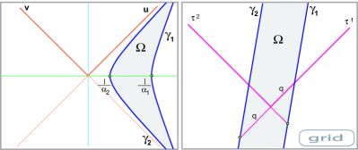
Figure 1: Trajectories of the uniformly accelerated emitters in flat space-time. (a) In inertial null coordinates $\{\texttt{u},\texttt{v}\}$. (b) In the grid $\{\tau^{1},\tau^{2}\}$; in this picture we have chosen the synchronization parameter $\sigma=0$.

III.2 Emitter’s positioning and dynamical parameters

Let us consider a user traveling on the emission domain $\Omega$ defined by this positioning system and receiving the emitter positioning data $\{\tau^{1},\tau^{2};\bar{\tau}^{1},\bar{\tau}^{2}\}$. Firstly, these data, under the form of the two sequences $\{\tau^{1},\bar{\tau}^{2}\}$ and $\{\bar{\tau}^{1},\tau^{2}\},$ determine the emitter trajectories $\varphi_{i}(\tau^{i})$ on the grid which, according to statement 1, will be straight lines, from which the user can extract the slope, separation and synchronization parameters $\omega>1$, $q>0$ and $\sigma$ (see (14) and (15)).

In fact, these parameters can be extracted from the emitter positioning data at two different events:

S.​​ 2

In terms of the emitter positioning data $\{\tau^{1}_{P},\tau^{2}_{P};\bar{\tau}^{1}_{P},\bar{\tau}^{2}_{P}\}$ and $\{\tau^{1}_{Q},\tau^{2}_{Q};\bar{\tau}^{1}_{Q},\bar{\tau}^{2}_{Q}\}$ at two different events $P$ and $Q$ of any user, the slope, separation and synchronization parameter $\omega>1$, $q>0$ and $\sigma,$ characterizing the parallel trajectories of the emitters in the grid $\{\tau^{1}\}\times\{\tau^{2}\}$, are given by:

$$\begin{array}[]{l}\displaystyle\omega=\frac{\Delta\bar{\tau}^{1}}{\Delta\tau^{2}}\equiv\frac{\bar{\tau}^{1}_{P}-\bar{\tau}^{1}_{Q}}{\tau^{2}_{P}-\tau^{2}_{Q}}\\[9.95845pt] \displaystyle q=\frac{1}{2}[\tau^{1}_{P}+\bar{\tau}^{1}_{P}+\frac{\Delta\bar{\tau}^{1}}{\Delta\tau^{2}}(\tau^{2}_{P}+\bar{\tau}^{2}_{P})]\\[9.95845pt] \displaystyle\sigma=\frac{1}{2}[\tau^{1}_{P}+\bar{\tau}^{1}_{P}-\frac{\Delta\bar{\tau}^{1}}{\Delta\tau^{2}}(\tau^{2}_{P}+\bar{\tau}^{2}_{P})]\end{array}$$ (18)

Once these parameters are evaluated, expression (16) implies that $\omega$ and $q$ determine one-to-one the acceleration of the emitters and (17) shows that the parameter $\sigma$ is necessary in obtaining the emitter synchronization:

S.​​ 3

For stationary positioning systems in Minkowski plane, the accelerations $\alpha_{1}$, $\alpha_{2}$ of the emitters may be obtained in terms of the slope data parameter $\omega>1$ and the separation data parameter $q>0,$ as:

$$\alpha_{1}=\frac{1}{q}\ln\omega\,,\qquad\alpha_{2}=\frac{\omega}{q}\ln\omega\ ,$$ (19)

and their synchronization times $\tau^{1}_{0}$ and $\tau^{2}_{0}$ indicated by the emitter clocks at two simultaneous events, are related to $\omega$ and the synchronization data parameter $\sigma$ by

$$\tau^{1}_{0}=\sigma+\omega\tau^{2}_{0}$$ (20)

This statement gives the parameters $\alpha_{1}$ and $\alpha_{2}$, as well as the relation between $\tau^{1}_{0}$ and $\tau^{2}_{0},$ in terms of the data parameters $\omega,$ $q$ and $\sigma$, which can be extracted from the data received by the user. Apart from their specific physical meaning, as accelerations and synchronization times of the emitters, these parameters $\alpha_{1},$ $\alpha_{2},$ $\tau^{1}_{0}$ and $\tau^{2}_{0},$ yield an operational definition of the null canonical inertial coordinates $\{\texttt{u},\texttt{v}\}$ associated with the emitters, i.e. those with origin in the intersection of the null asymptotes of the stationary system to which the emitters belong. This operational definition is offered by relations (12). Every set $\{\texttt{u},\texttt{v}\}$ of null coordinates so determined by (12) is one-to-one related to a standard inertial coordinate system $\{t,x\},$ by $\texttt{u}=t+x,$ $\texttt{v}=t-x$, and inertial systems of fixed origin are related by a one-parametric Lorentz transformation. It is such a parameter (say $\tau_{0}^{2}$ here) that relations (19) and (20) leave free for given data parameters $\omega$, $q$ and $\sigma.$

III.3 Metric in emission coordinates

Now, let us analyze the metric information that any user can obtain from the emitter positioning data. The expression of the metric function in emission coordinates follows from the coordinate transformation (12):

$$m(\tau^{1},\tau^{2})=u_{1}^{\prime}(\tau^{1})v_{2}^{\prime}(\tau^{2})=\exp[\alpha_{1}\tau^{1}-\alpha_{2}\tau^{2}-\alpha_{1}\sigma]$$ (21)

Consequently, by using (19), we can write the metric function in terms of the data $\{\tau^{1},\tau^{2}\}$ and the parameters $\{\omega,q,\sigma\}$:

S.​​ 4

In Minkowski plane, the space-time metric in emission coordinates of a stationary positioning system is given, in terms of the emitter positioning data $\{\tau^{1},\tau^{2};\bar{\tau}^{1},\bar{\tau}^{2}\},$ by:

$$ds^{2}=\exp\left[\frac{\ln\omega}{q}(\tau^{1}-\omega\tau^{2}-\sigma)\right]d\tau^{1}d\tau^{2}$$ (22)

where the data parameters $\omega$, $q$, $\sigma$ can be obtained by (18) in terms of the values of these data at two events.

This statement shows that the sole public quantities $\{\tau^{1},\tau^{2};\bar{\tau}^{1},\bar{\tau}^{2}\}$ received by any user allow him to know the space-time metric everywhere. Nevertheless, it is worth remarking that, in order for a user to obtain this result, the user must be informed that the emitter positioning data come from a stationary positioning system in absence of gravitational fields. Otherwise, the above deduction based on the existence of the coordinate transformation (12) would not be valid. Remark also that this required information does not demand the specific value of the accelerations of the emitters, which may be also determined by the user by relations (19).

The users may know that the system of the two emitter clocks is stationary by an a priori information, forming part of the dynamical characteristics of the positioning system and its foreseen control. But they may also obtain this information in real time, if clocks and users are endowed with devices allowing the users to know the emitter accelerations $\{\alpha_{1},\alpha_{2}\}$ at every instant (see comments in sections V and VII and Ref. cfm-c )

In any case, the user information of the dynamics of the pair of clocks by any of these two methods is generically necessary, because emitter trajectories that are parallel straight lines in the grid are not necessarily uniformly accelerated trajectories in a flat space-time cfm-c . In Sec. IV we show that in a non flat space-time we can also find in the grid the same picture that Fig. 1(b).

III.4 Stationary user

The considerations that follow in this section are qualitatively independent of the synchronization of the emitters. For this reason, we assume for the sake of simplicity the synchronization parameter to be zero, $\sigma=0$.

All the above considerations are valid for any user $\gamma$ which, as we have already said, can also obtain from the user positioning data $\{\tau^{1},\tau^{2}\}$ his own trajectory in the grid. Then, the expression (22) of the metric tensor allows him to calculate as usual his proper time lapse and acceleration in terms of the emitter positioning data $\{\tau^{1},\tau^{2};\bar{\tau}^{1},\bar{\tau}^{2}\}$.

Suppose now that a user obtains from these data the following trajectory:

$$\tau^{2}=F(\tau^{1})=\frac{1}{\omega}(\tau^{1}-c)\,,\qquad-q<c<q\,,$$ (23)

that is, a straight line parallel to the emitter trajectories [see Fig. 2(a), where we plot the case $c=0$]. What is his dynamics and his relation to the emitters? The answer is given by [see Fig. 2(b)]:

S.​​ 5

The users which find that their trajectory in the grid is a straight line parallel to the emitter ones [Eq. (23)], are the users which are stationary with respect to the emitters. Their acceleration is the weighted geometric mean of the emitters’ accelerations:

$$\alpha\equiv\sqrt{\alpha_{1}^{1+c/q}\,\alpha_{2}^{1-c/q}},$$ (24)

and their proper time lapse $\Delta\tau$ is, for any of the two emitter clocks (no summation)

$$\Delta\tau=\frac{\alpha_{i}}{\alpha}\Delta\tau^{i}.$$ (25)

To obtain these results, let us construct as above indicated the canonical inertial coordinate systems $\{\texttt{u},\texttt{v}\}$ associated with the emitters. The transformation equations from the emission coordinates $\{\tau^{1},\tau^{2}\}$ to these inertial coordinates are given by (12). In them, using the inverse transformation (13), the trajectory equation (23) becomes:

$$\texttt{u}\texttt{v}=-\frac{1}{\alpha^{2}}\,,$$ (26)

where the constant $\alpha$ is given by (24). This means that this trajectory belongs to the stationary family of trajectories that contains that of the two emitters, and that its constant acceleration is $\alpha.$ To finish the proof of the statement 5 we consider the proper time parametrization of the stationary user (26):

$$\!\gamma\equiv\begin{cases}\,\displaystyle\texttt{u}=u(\tau)=\frac{1}{\alpha}\exp[\alpha(\tau-\tau_{0})]\\[8.53581pt] \,\displaystyle\texttt{v}=v(\tau)=-\frac{1}{\alpha}\exp[-\alpha(\tau-\tau_{0})]\end{cases}$$ (27)

Then, (27) and the coordinate transformation (12) give the expression (25) of the proper time lapse of the user.

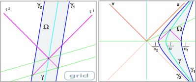
Figure 2: (a) The user positioning data $\{\tau^{1},\tau^{2}\}$ determine the trajectory of the user $\gamma$ in the grid: $\tau^{2}=\frac{1}{\omega}\tau^{1}$. The parallel straight lines $\tau^{2}=-\frac{1}{\omega}\tau^{1}+C$ are the locus of simultaneous events for the uniformly accelerated emitters. (b) Trajectory of the user $\gamma$ in inertial null coordinates $\{\texttt{u},\texttt{v}\}$: he also has an hyperbolic motion.

III.5 Simultaneous events for the emitters

In order to better understand the grid associated with the emission coordinates of our two-dimensional stationary positioning systems, let us consider the locus of simultaneous events for both emitters, i.e. the orthogonal lines to the stationary family of trajectories that contains that of the two emitters which, as it is well known, are the space-like geodesics cutting at the common point of the two asymptotes of the emitters. How can they be constructed in the grid? The answer is:

S.​​ 6

The locus of simultaneous events for the emitters of a stationary positioning system in Minkowski plane are parallel straight lines of slope $-\frac{1}{\omega}$, the same, up to sign, as that of the trajectory of the emitters.

To see this, take into account that in inertial null coordinates these lines are $\texttt{u}=-\kappa\texttt{v}\ ,\kappa>0$. It is then sufficient to change to emission coordinates using (12) to obtain:

$$\tau^{2}=-\frac{1}{\omega}\tau^{1}+C,\qquad C\equiv\frac{1}{\alpha_{2}}\ln\frac{\kappa}{\omega}+2\tau_{0}^{2}$$

which shows directly the statement [see Fig. 2(a)].

III.6 Geodesic user

To finish this section, let us consider the user positioning data received by an inertial (geodesic) user. For simplicity, but with no qualitative differences, we shall choose him to be at rest with respect to the emitters at the initial instant at which $\tau^{1}_{0}=\tau^{2}_{0}=0$ (remember that we have taken $\sigma=0$). For him we have:

S.​​ 7

The trajectory in emission coordinates of inertial users initially at rest with respect to two synchronized stationary emitters is:

$$\tau^{2}=F(\tau^{1})=-\frac{1}{\alpha_{2}}\ln[A-\omega\exp[\alpha_{1}\tau^{1}]]\,,$$ (28)

where $A$ is a constant.

This equation may be obtained as follows. Choose the null inertial system $\{\texttt{u},\texttt{v}\}$ associated with the inertial observer having the same initial instant as the two emitters, that is to say, such that $\tau^{1}_{0}=\tau^{2}_{0}=0.$ Because the user is at rest with respect this null inertial system, its trajectory is given by [see Fig. 3(a)]:

$$\texttt{v}=\texttt{u}-2x_{0}\,,\qquad x_{0}<\frac{1}{\alpha_{2}}$$ (29)

Then, making use of the coordinate transformation (12), a straightforward calculation leads to expression (28), with $A\equiv 2x_{0}\alpha_{2}$. Note that the coordinate $\tau^{2}$ run in $]-\frac{1}{\alpha_{2}}\ln A,+\infty[$ when $\tau^{1}$ run in $]-\infty,\frac{1}{\alpha_{1}}\ln(A/\omega)\ [$. Thus the data $\{\tau^{1},\tau^{2}\}$ of a geodesic user lead to a trajectory in the grid with a double asymptotic behavior [see Fig. 3(b)].

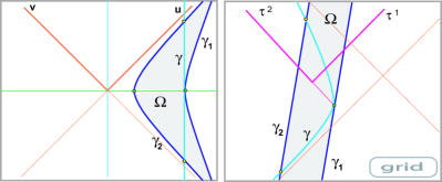
Figure 3: Trajectory of a geodesic user $\gamma$ with $x_{0}=\frac{1}{\alpha_{1}}$: (a) In inertial null coordinates $\{\texttt{u},\texttt{v}\}$. (b) In the grid $\{\tau^{1},\tau^{2}\}$ defined in flat space-time by two uniformly accelerated emitters.

IV Positioning in Schwarzschild plane

In this section we study stationary positioning systems defined by two emitters at rest with respect to the gravitational field in Schwarzschild plane.

The usual expression for the space-time metric in the exterior region to the Schwarzschild radius $r_{s}$ is:

$$ds^{2}=b(r)d\bar{t}^{2}-\frac{1}{b(r)}dr^{2}\ ,\qquad b(r)\equiv 1-\frac{r_{s}}{r}$$

We can introduce the stationary time $t$ and the radial coordinate $\rho$ from the horizon, both in units of Schwarzschild radius:

$$t=\frac{\bar{t}}{r_{s}}\,,\qquad\quad\rho=\frac{r}{r_{s}}-1>0$$ (30)

To obtain a conformally flat expression for the metric, one can change the radial coordinate $\rho$ for the new one $x$:

$$x=x(\rho)\equiv\rho+\ln\rho$$ (31)

The inverse function that gives the coordinate $\rho$ in terms of $x$ may be expressed by using the Lambert function $w=W(z)$, which is defined as the inverse of the function $z=w\exp w$. Indeed, from (31) we have:

$$\rho=\rho(x)\equiv W(\exp x)$$ (32)

Finally, one can define the stationary null coordinates $\{\texttt{u},\texttt{v}\}$ [see Fig. 4(a)]:

$$\begin{array}[]{ll}\texttt{u}=t+x&\qquad\qquad t=\frac{1}{2}(\texttt{u}+\texttt{v})\\[2.84526pt] \texttt{v}=t-x&\qquad\qquad x=\frac{1}{2}(\texttt{u}-\texttt{v})\end{array}$$ (33)

With all these transformations one obtains:

In the exterior region, the metric of Schwarzschild plane takes the expression:

$$ds^{2} = r_{s}^{2}\,b(\rho)\,d\texttt{{\rm u}}\,d\texttt{{\rm v}}$$ (34)

$$b(\rho)\equiv\frac{\rho}{\rho+1}\,, \rho\equiv W\left(\exp\left[\frac{\texttt{{\rm u}}-\texttt{{\rm v}}}{2}\right]\right)$$ (35)

where $W(z)$ is the Lambert function.

The trajectories of two stationary emitters $\gamma_{i}$ are defined by the conditions [see Fig. 4(a)]:

$$\rho=\rho_{i}\ ,\qquad 1<\rho_{2}<\rho_{1}$$ (36)

The method exposed in Sec. II to introduce emission coordinates is based in obtaining the metric tensor in a null coordinate system, as expressions (34) and (35) do, and in knowing the proper time history of the emitters in this system. In coordinates $\{\texttt{u},\texttt{v}\}$ for the two trajectories (36) one has, by (31) and (33), $\dot{\texttt{u}}=\dot{\texttt{v}}$ and then from (34) the unit character of their velocity gives $r_{s}^{2}\,b(\rho_{i})\,\dot{\texttt{u}}^{2}=1$. Consequently, the two trajectories are given by (the repeated index does not indicate summation):

$$\gamma_{i}\equiv\begin{cases}\,\texttt{u}=u_{i}(\tau^{i})=\lambda_{i}(\tau^{i}-\tau^{i}_{0})+x_{i}\\[2.84526pt] \,\texttt{v}=v_{i}(\tau^{i})=\lambda_{i}(\tau^{i}-\tau^{i}_{0})-x_{i}\end{cases}$$ (37)

where the constants $\lambda_{i}$ and $x_{i}$ depend exclusively on The Schwarzschild radius $r_{s}$ and the radial parameter $\rho_{i}$:

$$\lambda_{i}=\frac{1}{r_{s}}\sqrt{\frac{\rho_{i}+1}{\rho_{i}}}\ ,\qquad x_{i}=x(\rho_{i})$$ (38)

and where $\tau^{i}_{0}$ are the proper times that indicate the emitter clocks at two events with the same Schwarzschild time $t$.

It is important to remark that the radial parameter $\rho_{i}$ is a dynamical characteristic of the trajectory, equivalent to the acceleration parameter $\alpha_{i}$. Indeed, as the emitter acceleration scalars are constant because emitter trajectories are tangent to a Killing vector, a standard computation of them gives:

$$\alpha_{i}=\frac{1}{2\,r_{s}\,\rho_{i}^{1/2}(\rho_{i}+1)^{3/2}}$$ (39)

Is is easy to see that this relation admits a unique real positive solution $\rho_{i}=\rho_{i}(\alpha_{i}),$ showing their one-to-one equivalence and, thus, the stated dynamical character of $\rho_{i}.$

IV.1 Emission coordinates and emitter trajectories

According to (8), the emission coordinates $\{\tau^{1},\tau^{2}\}$ are defined by the transformation to the stationary null system $\{\texttt{u},\texttt{v}\}$:

$$\begin{array}[]{l}\texttt{u}=u_{1}(\tau^{1})=\lambda_{1}(\tau^{1}-\tau^{1}_{0})+x_{1}\\[5.69054pt] \texttt{v}=v_{2}(\tau^{2})=\lambda_{2}(\tau^{2}-\tau^{2}_{0})-x_{2}\end{array}$$ (40)

and the inverse transformation is:

$$\begin{array}[]{l}\displaystyle\tau^{1}=\tau^{1}_{0}+\frac{1}{\lambda_{1}}(\texttt{u}-x_{1})\\[5.69054pt] \displaystyle\tau^{2}=\tau^{2}_{0}+\frac{1}{\lambda_{2}}(\texttt{v}+x_{2})\end{array}$$ (41)

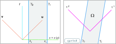
Figure 4: Trajectories of stationary emitters in Schwarzschild plane. (a) In ‘stationary’ null coordinates $\{\texttt{u},\texttt{v}\}$ associated with the static time $t$ and the coordinate $x=x(\rho)$. The stationary observers are defined by $\texttt{v}=\texttt{u}+constant$. (b) In the emission grid $\{\tau^{1},\tau^{2}\}$.

Making use of (10), we can obtain the expression of the emitter trajectories in emission coordinates $\{\tau^{1},\tau^{2}\}$:

S.​​ 8

In Schwarzschild plane, the trajectories $\gamma_{1}$, $\gamma_{2}$ of the emitters of a stationary positioning system in emission coordinates $\{\tau^{1},\tau^{2}\}$ are parallel straight lines of the form:

$$\gamma_{1}\equiv\begin{cases}\tau^{1}=\tau^{1}\\ \tau^{2}=\frac{1}{\omega}(\tau^{1}-q-\sigma)\equiv\varphi_{1}(\tau^{1})\end{cases}\,$$ (42)

$$\gamma_{2}\equiv\begin{cases}\tau^{1}=\omega\tau^{2}-q+\sigma\equiv\varphi_{2}(\tau^{2})\\ \tau^{2}=\tau^{2}\end{cases}\quad$$ (43)

The slope parameter $\omega$, the separation parameter $q$ and the synchronization parameter $\sigma$ are related to the Schwarzschild radius $r_{s}$, the radial parameters $\rho_{i}$ and the synchronization instants $\tau^{i}_{0}$ of the emitters by:

$$\begin{array}[]{l}\displaystyle\omega=\frac{\lambda_{2}}{\lambda_{1}}=\omega(\rho_{1},\rho_{2})\\[9.95845pt] \displaystyle q=\frac{x_{1}-x_{2}}{\lambda_{1}}=r_{s}Q(\rho_{1},\rho_{2})\\[9.95845pt] \sigma=\tau^{1}_{0}-\omega\tau^{2}_{0}\end{array}$$ (44)

$\omega(\rho_{1},\rho_{2})$ and $Q(\rho_{1},\rho_{2})$ being the bi-parametric expressions:

$$\begin{array}[]{l}\displaystyle\omega(\rho_{1},\rho_{2})\equiv\sqrt{\frac{\rho_{1}(\rho_{2}+1)}{\rho_{2}(\rho_{1}+1)}}\\[11.38109pt] \displaystyle Q(\rho_{1},\rho_{2})\equiv\sqrt{\frac{\rho_{1}}{\rho_{1}+1}}\left[\rho_{1}-\rho_{2}+\ln\frac{\rho_{1}}{\rho_{2}}\right]\end{array}$$ (45)

Fig. 4(b) illustrates these trajectories in the grid.

IV.2 Emitter’s positioning and dynamical parameters

As a consequence of the above statement, any user traveling on the emission coordinate domain $\Omega$ of this positioning system and receiving the emitter positioning data $\{\tau^{1},\tau^{2};\bar{\tau}^{1},\bar{\tau}^{2}\}$ can find a particular linear relation between the $\bar{\tau}$’s and the $\tau$’s, leading him to find that the emitter trajectories $\varphi_{i}(\tau^{i})$ are parallel straight lines in the grid of the emission coordinates he is receiving. From them, he can extract the parameters $\omega>1$, $q>0$ and $\sigma$ [see (42) and (43)]:

S.​​ 9

The slope, separation and synchronization parameters $\omega>1$, $q>0$ and $\sigma,$ characterizing the parallel trajectories in the grid $\{\tau^{1}\}\times\{\tau^{2}\}$ of the stationary emitters in Schwarzschild plane have, in terms of the emitter positioning data at two different events $P$ and $Q$, the same expression as in Minkowski plane, given by (18).

Once these parameters are evaluated, expressions (44) and (45) tell us that $\omega$ and $q$ determine one-to-one the dynamical radial parameters $\rho_{i}$, which characterize the emitter trajectories. Indeed, from the first expression in (45) we can obtain:

$$\rho_{2}=\frac{\rho_{1}}{(\omega^{2}-1)\rho_{1}+\omega^{2}}$$ (46)

and, substituting in the second one, we have:

$$Q(\rho_{1};\omega)\equiv\sqrt{\frac{\rho_{1}}{\rho_{1}+1}}\left[\frac{\rho_{1}(\rho_{1}+1)}{\rho_{1}+\frac{\omega^{2}}{\omega^{2}-1}}+\ln[(\omega^{2}-1)\rho_{1}+\omega^{2}]\right]$$ (47)

This expression of $Q(\rho_{1},\omega)$ is an effective function on $\rho_{1}$. Consequently it admits an inverse and this radial parameter may be obtained as a function of $\omega$ and $Q\equiv q/r_{s}$.

Moreover, the third expression in (44) shows that the parameter $\sigma$ gives the emitter synchronization. All these results can be summarized in the following:

S.​​ 10

For stationary positioning systems in Schwarzschild plane, the radial parameters $\rho_{1}$, $\rho_{2}$ of the emitters may be obtained in terms of the slope data parameter $\omega>1$ and the separation data parameter $q>0,$ by (46) and

$$\rho_{1}=\rho_{1}(\omega,q/r_{s})\,,$$ (48)

where $\rho_{1}(\omega,q/r_{s})$ is the inverse of (47).

Also, their synchronization times $\tau^{1}_{0}$ and $\tau^{2}_{0}$ indicated by the emitter clocks at two simultaneous events, are related to $\omega$ and the synchronization data parameter $\sigma$ by

$$\tau^{1}_{0}=\sigma+\omega\tau^{2}_{0}$$ (49)

This statement gives the parameters $\rho_{1}$ and $\rho_{2}$, as well as the relation between $\tau^{1}_{0}$ between $\tau^{2}_{0},$ in terms of the data parameters $\omega,$ $q$ and $\sigma$, which can be extracted from the data received by the user. In analogy to Minkowskian case, these parameters yield an operational definition of the null canonical stationary coordinates $\{\texttt{u},\texttt{v}\}$ associated with the emitters and given by (40). By (48) and (49) these coordinates depend on a unique parameter (say $\tau^{2}_{0}$), which now controls the time-like translations in the direction $\texttt{u}+\texttt{v}$.

IV.3 Metric in emission coordinates

What is the metric information that the emitter positioning data offer to the users? To obtain the metric function in emission coordinates, starting from (34) and using the coordinate transformation (40), one obtains:

$$\begin{array}[]{lcl}m(\tau^{1},\tau^{2})&=&r_{s}^{2}\,b(\tau^{1},\tau^{2})u_{1}^{\prime}(\tau^{1})v_{2}^{\prime}(\tau^{2})\\[5.69054pt] &=&r_{s}^{2}\,b\left(\rho(x(\tau^{1},\tau^{2}))\right)\lambda_{1}\lambda_{2}\end{array}$$ (50)

But from (40) and (44) we have:

$$\begin{array}[]{lcl}2x(\tau^{1},\tau^{2})&=&u_{1}(\tau^{1})-v_{2}(\tau^{2})\\[5.69054pt] &=&\lambda_{1}(\tau^{1}-\omega\tau^{2}-\sigma-q)+2x(\rho_{1})\end{array}$$ (51)

So that, by using (38) and (48), we can write the metric function in terms of the data $\{\tau^{1},\tau^{2}\}$ and the parameters $\{\omega,q,\sigma\}$. Moreover these parameters can be obtained as in (18) from the emitter positioning data $\{\tau^{1}_{P},\tau^{2}_{P};\bar{\tau}^{1}_{P},\bar{\tau}^{2}_{P}\}$ and $\{\tau^{1}_{Q},\tau^{2}_{Q};\bar{\tau}^{1}_{Q},\bar{\tau}^{2}_{Q}\}$ at two events $P$ and $Q$. Thus, we can state:

S.​​ 11

In Schwarzschild plane, the space-time metric in emission coordinates of a stationary positioning system is given, in terms of the emitter positioning data $\{\tau^{1},\tau^{2};\bar{\tau}^{1},\bar{\tau}^{2}\},$ by:

$$\displaystyle ds^{2}=\frac{1+\rho_{1}}{\rho_{1}}\omega\,b(\tau^{1},\tau^{2})\,d\tau^{1}d\tau^{2}$$ (52)

where

$$b(\tau^{1},\tau^{2})\equiv\frac{W(\exp x(\tau^{1},\tau^{2}))}{1+W(\exp x(\tau^{1},\tau^{2}))}\,,$$

$W(z)$ being the Lambert function and

$$x(\tau^{1},\tau^{2})\equiv\frac{1}{2r_{s}}\sqrt{\frac{1+\rho_{1}}{\rho_{1}}}(\tau^{1}-\omega\tau^{2}-\sigma-q)+\rho_{1}\ln\rho_{1},$$

where the parameters $\{\omega,q,\sigma\}$ are given by (18) in terms of the values of the data at two events, and the constant $\rho_{1}$ is defined in (48).

This statement shows that the sole public quantities $\{\tau^{1},\tau^{2};\bar{\tau}^{1},\bar{\tau}^{2}\}$ received by any user allow him to know the space-time metric everywhere. It is worth remarking that the user must be informed that the emitter positioning data come from a stationary positioning system in presence of a mass of the Schwarzschild radius $r_{s}$. Remark also that this information does not require the specific value of the emitter radial parameters $\rho_{i}$, which may be determined by the user from the relations (46) and (48).

As statements 1 and 8 show, the sole emitter positioning data $\{\tau^{1},\tau^{2};\bar{\tau}^{1},\bar{\tau}^{2}\}$ give the same picture in the grid in Minkowski and in Schwarzschild planes. Consequently, the additional quantitative information of The Schwarzschild radius $r_{s}$ is a necessary information in order to obtain the metric and the dynamical quantities. Moreover, as we have already commented for Minkowski plane, the user’s knowledge of the accelerations of the clocks is generically necessary because different dynamics (including non uniformly accelerated ones) may produce the same emitter trajectories in the grid cfm-c . On the other hand, we will show in next section that the data of one of the emitter’s accelerations allows the user to determine Schwarzschild mass.

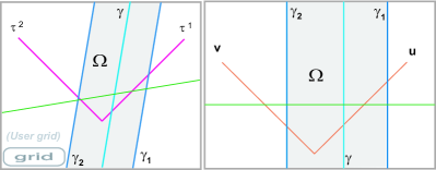
Figure 5: (a) User $\gamma$ with a trajectory in the grid parallel to the stationary emitters in Schwarzschild plane. Note that parallel straight lines $\tau^{2}=-\frac{1}{\omega}\tau^{1}+C$ are the hypersurfaces with Schwarzschild time $t=constant$. (b) Trajectory of the user $\gamma$ in ‘stationary’ null coordinates $\{\texttt{u},\texttt{v}\}$: it is an stationary user.

IV.4 Stationary user

All the results above are independent of the user motion. Let us consider now the specific user $\gamma$ which obtains from the public data $\{\tau^{1},\tau^{2}\}$ his own trajectory in the grid as [see Fig. 5(a)]:

$$\tau^{2}=F(\tau^{1})=\frac{1}{\omega}(\tau^{1}-c)\,,\qquad-q<c-\sigma<q\,,$$ (53)

that is, a straight line parallel to the emitter trajectories. The dynamics of this user and its relation with the emitters are given by [see Fig. 5(b)]:

S.​​ 12

The users which find that their trajectory in the grid is a straight line parallel to the emitter’s ones [Eq. (23)] are stationary users in Schwarzschild plane. Their radial parameter $\bar{\rho}$ is:

$$\bar{\rho}=W(\exp\bar{x}),\qquad\bar{x}\equiv\frac{1}{2}[x_{1}+x_{2}+\lambda_{1}(c-\sigma)],$$ (54)

their constant acceleration scalar $\alpha$ is

$$\alpha=\frac{1}{2r_{s}\,\bar{\rho}^{1/2}(\bar{\rho}+1)^{3/2}}$$ (55)

and their proper time lapse $\Delta\tau$ is, for any of the two emitter clocks (no summation)

$$\Delta\tau=\frac{\lambda_{i}}{\lambda}\Delta\tau^{i},\qquad\lambda=\frac{1}{r_{s}}\sqrt{\frac{\bar{\rho}+1}{\bar{\rho}}}.$$ (56)

Observe that the parameters $x_{i}$, $\lambda_{i}$ and $\sigma$, and then the value of the radial parameter $\bar{\rho}$ of the user depend on the emitter positioning data $\{\tau^{1},\tau^{2};\bar{\tau}^{1},\bar{\tau}^{2}\}$ and The Schwarzschild radius $r_{s}$, as a consequence of (38), (46) and (48).

In order to show these relations, let us construct, starting from the emitter positioning data, the stationary null coordinate system $\{\texttt{u},\texttt{v}\}$ given by (40). In it, using the inverse transformation (41), the trajectory equation (53) becomes:

$$\texttt{u}-\texttt{v}=2\bar{x}$$ (57)

where $\bar{x}$ is given in (54). This means that this trajectory belongs to the stationary family of trajectories as the statement says.

Furthermore, the user can also obtain, up to an origin, his own proper time $\tau$. Indeed, in the null coordinate system $\{\texttt{u},\texttt{v}\}$ the proper time user trajectory is:

$$\gamma\equiv\begin{cases}\,\texttt{u}=\lambda(\tau-\tau_{0})+\bar{x}\\ \,\texttt{v}=\lambda(\tau-\tau_{0})-\bar{x}\end{cases}$$ (58)

where the constant $\lambda$ is given by the second of expressions (56).

Then, (58) and the coordinate transformation (40) imply the first of expressions (56).

IV.5 Simultaneous events for the emitters

The simultaneity loci of the stationary emitters in stationary null coordinates are given by the lines $\texttt{u}+\texttt{v}=2t=constant$. Using the coordinate transformation (40) one obtains that these loci take in the grid the following expression:

$$\tau^{2}=-\frac{1}{\omega}\tau^{1}+C.$$

Thus, as in the flat case, one has:

S.​​ 13

The locus of simultaneous events for the emitters of a stationary positioning system in Schwarzschild plane are parallel straight lines of slope $-\frac{1}{\omega}$, the same, up to sign, as that of the trajectory of the emitters.

IV.6 Comparing Minkowski

It is worth remarking that the emitter positioning data received by a user give, in the two physically different two-dimensional Minkowski and Schwarzschild space-times, the same qualitative information about the emitter trajectories in the grid, as we have seen in this and the precedent section [see Figs. 1(b) and 4(b)]. Moreover, the trajectory in the grid of any stationary user is also the same in both cases [see Figs. 2(a) and 5(a)]. In spite of this fact, we shall see in the next section that complementary data that afford dynamic information of the system allow the user to distinguish between both systems.

The relevance of the dynamical data for the determination of the system is manifest in the case of a geodesic user: his trajectory in the grid is different in both cases. Is is easy to show this fact because the trajectory (28) of a geodesic user in the grid of the system in the flat case is not geodesic for the Schwarzschild metric (34), as a straightforward calculation shows. In this last case the geodesics, qualitatively similar to those of the flat case shown in Fig. 3(b), have nevertheless a different trajectory equation. By comparison of this trajectory with the one constructed by the geodesic user from the received sole data $\{\tau^{1},\tau^{2}\}$, he is able to distinguish in which space-time he is evolving.

V Gravimetry and positioning: the information of the user data

The interest of auto-locating positioning systems in gravimetry has been pointed out in cfm-a , where we have shown that, if a user has neither a priori information on the gravitational field nor on the positioning system, the user data determine the metric and its first derivatives along the user and emitter trajectories. In the next section we apply these results to obtain the gravitational information that can be extracted from the user data generated by the positioning systems of the precedent sections.

But in some cases the user can have some a priori information about the space-time or about the kind of positioning system he is using. The different levels of not null information in these two aspects establishes different kinds of gravity problems. For example, in the last two precedent sections, we have supposed the space-time fully known (Minkowski or Schwarzschild planes), and also the partial information on the positioning system assuring its stationarity, but without specifying the space-time trajectories of the emitters.

In this section we will consider other situations of total or partial information on the space-time itself and/or on the positioning system, and we will analyze the role that the emitter accelerations and the proper user data can play in obtaining the gravitational field and in recovering the complementary characteristics of the positioning system.

We consider two levels in the a priori information that the user can have about the gravitational field. He may know generically that:

• (GF-1) The space-time belongs to the family of Schwarzschild planes expanded to include Minkowski plane,

or specifically that:

• (GF-2) The space-time is a particular Schwarzschild plane with a known the Schwarzschild radius $r_{s}$ or it is Minkowski plane.

We also consider two levels in the a priori user information about the positioning system. He may know generically that:

• (PS-1) The positioning system is defined by two stationary emitters,

or specifically that:

• (PS-2) The positioning system is defined by two particular stationary emitters with known radial coordinates $\rho_{i}$ and a fixed synchronization $\sigma$.

V.1 A user with full a priori information

If the user has the widest information (GF-2) about the gravitational field and the widest information (PS-2) about the positioning system, then, from (GF-2) he can take a convenient coordinate system and express in it the metric components and from (PS-2) he can describe in this coordinate system the trajectory of the emitters and the future light rays that spread from them. Then, he may construct the emission coordinates and calculate the coordinate transformation relating them to the initial ones. Consequently, he can evaluate the emitter trajectories and the space-time metric in emission coordinates. Thus, without receiving any data, the user can know by calculation the pairs $\{\tau^{1},\bar{\tau}^{2}\}$ and $\{\tau^{2},\bar{\tau}^{1}\}$ locating the emitters as well as their dynamics.

With this full information about the metric and the positioning system, a user receiving the user positioning data $\{\tau^{1},\tau^{2}\}$ may extract his trajectory $\tau^{2}=F(\tau^{1})$ in the grid. Moreover at every event $(\tau^{1},\tau^{2})$ on his trajectory, he may know the metric function $m(\tau^{1},\tau^{2})$ and his acceleration.

Thus, in particular, the user may obtain his own units of time and distance. For example, in the particular case of a stationary user, his proper time is given by (56).

V.2 A user with full metric information and partial knowledge of the positioning system

The situation in which a user has the widest information about the gravitational field (GF-2) and partial information about the positioning system (PS-1) is the one that has been analyzed in detail in Sec. III for Minkowski plane and in Sec. IV for Schwarzschild plane.

In particular, we have shown that the sole emitter positioning data $\{\tau^{1},\tau^{2};\bar{\tau}^{1},\bar{\tau}^{2}\}$ complete the system information [see statements 3 and 10]. Moreover we have shown that the space-time metric may be obtained in terms of these data (see statements 4 and 11).

Once completed the system information in this way, the user is in the situation of the precedent subsection and, as commented there, he can also obtain his trajectory and his own units of time and distance.

V.3 Obtaining The Schwarzschild mass from the emitter accelerations

Suppose now that the user has partial information (GF-1) about the gravitational field and also partial information (PS-1) about the positioning system. The user knows thus that the system is defined by stationary emitters and, consequently, that they have constant acceleration. If the emitters carry accelerometers and broadcast their accelerations, the user can receive the precise value $\alpha_{1}$ $\alpha_{2}$ of these accelerations.

Can this dynamical information determine The Schwarzschild mass? The answer is affirmative. Furthermore, apart from the emitter positioning data $\{\tau^{1},\tau^{2};\bar{\tau}^{1},\bar{\tau}^{2}\}$, only one of the two accelerations is sufficient to the user to obtain The Schwarzschild mass and, consequently, to acquire the information level considered in the precedent subsections.

In order to specify exactly this result let us assume firstly that the user knows the full set of the public data $\{\tau^{1},\tau^{2};\bar{\tau}^{1},\bar{\tau}^{2};\alpha_{1},\alpha_{2}\}$. We know that the data parameters $\{\omega,q,\sigma\}$ depend on the emitter positioning data [see (18)]. Because the accelerations $\alpha_{i}$ are also known, the first expression in (45) and the the two in (39) constitute three relations in $\{r_{s},\rho_{1},\rho_{2}\}$ that allow to obtain them explicitly in terms of $\{\omega,\alpha_{1},\alpha_{2}\}$. On the other hand, the resulting expressions have to be compatible with the expression of $q$ given in (44).

In the case of Minkowski plane, the user data parameters $\{\omega,q,\alpha_{1},\alpha_{2}\}$ are submitted not to one but to two compatibility conditions, those given by (16). This fact and the considerations in the above paragraph lead to the following

S.​​ 14

Consider a user of a stationary positioning system in a space-time of which he only knows that it is either a Schwarzschild or Minkowski plane. Let $\{\tau^{1},\tau^{2};\bar{\tau}^{1},\bar{\tau}^{2};\alpha_{1},\alpha_{2}\}$ be the public data that he receives, $\{\omega,q,\sigma\}$ the data parameters that can be extracted from them by means of (18), and $\kappa$ the data parameter given by:

$$\kappa\equiv\sqrt{\frac{\omega\alpha_{1}}{\alpha_{2}}}.$$ (59)

Then $\kappa$ is necessarily such that:

$$\kappa\leq 1.$$ (60)

Moreover:

(i) The value $\kappa=1$ is the one that informs the user that his space-time is Minkowski plane. In this case, the public data are submitted to the constraints:

$$\alpha_{1}\omega=\alpha_{2}\,,\qquad q\alpha_{1}=\ln\omega$$ (61)

(ii) Any value $\kappa<1$ informs the user that his space-time is Schwarzschild plane with radius

$$r_{s}=\frac{(\omega^{2}-1)^{2}}{2\,\alpha_{2}(1-\kappa)^{1/2}(\omega^{2}-\kappa)^{3/2}},$$

that the radial coordinate of the emitters are:

$$\rho_{1}=\frac{\omega^{2}(1-\kappa)}{\kappa(\omega^{2}-1)}\,,\qquad\rho_{2}=\frac{1-\kappa}{\omega^{2}-1},$$

and that the public data are submitted to the constraint:

$$2q\alpha_{1}\frac{\omega^{2}-\kappa}{\kappa(\omega^{2}-1)}=1-\kappa+\frac{\kappa(\omega^{2}-1)}{\omega^{2}-\kappa}\ln\frac{\omega^{2}}{\kappa}$$ (62)

The compatibility condition (62) for the data parameters $\{\omega,q,\alpha_{1},\alpha_{2}\}$ suggests that the emitter positioning data $\{\tau^{1},\tau^{2};\bar{\tau}^{1},\bar{\tau}^{2}\}$ and a sole acceleration, say $\alpha_{1}$, are sufficient data to determine The Schwarzschild mass. Indeed, from (39) we obtain:

$$r_{s}=\frac{1}{2\,\alpha_{1}\,\rho_{1}^{1/2}(\rho_{1}+1)^{3/2}}$$ (63)

This expression allows eliminate $r_{s}$ in the expression (44) of $q$, which becomes:

$$q = \frac{1}{2\alpha_{1}}\Theta(\rho_{1},\rho_{2})$$ (64)

$$\Theta(\rho_{1},\rho_{2}) \equiv \frac{1}{(\rho_{1}+1)^{2}}\left[\rho_{1}-\rho_{2}+\ln\frac{\rho_{1}}{\rho_{2}}\right]$$ (65)

Then, substituting (46) in (65), (64) takes the form:

$$2q\alpha_{1}=\Theta(\rho_{1},\omega)\,.$$ (66)

This expression of $\Theta(\rho_{1},\omega)$ is an effective function on $\rho_{1}.$ Consequently it admits an inverse:

$$\rho_{1}=\rho_{1}\left(\omega,q\alpha_{1}\right)\,,$$ (67)

and we can state:

S.​​ 15

Consider a user of a stationary positioning system in a space-time of which he only knows that it is a Schwarzschild plane. Let $\{\tau^{1},\tau^{2};\bar{\tau}^{1},\bar{\tau}^{2}\}$ be the emitter positioning data that he receives and suppose that he also receives but one of the emitter dynamical data, say $\alpha_{1}$. Then, The Schwarzschild radius $r_{s}$ is given by (63) where $\rho_{1}$ may be extracted from (66) as (67), in terms of the data parameters $\{\omega,q,\alpha_{1}\}$.

V.4 Obtaining The Schwarzschild mass from the user’s proper time

Let us assume again that the user has partial information (GF-1) and (PS-1) respectively about the gravitational field and the positioning system. We show here that if the user is stationary and generates his proper time, he can also obtain the Schwarzschild mass.

Let us suppose that a user receiving the emitter positioning data $\{\tau^{1},\tau^{2};\bar{\tau}^{1},\bar{\tau}^{2}\}$ carries a clock that measures his proper time $\tau$ and that he is stationary with respect to the stationary positioning system. Remember that, from statement 5, he knows that he is stationary if his trajectory in the grid is parallel to the trajectories of the stationary emitters and that this property may be extracted from the user positioning data he is receiving. From his trajectory in the grid, he may also extract by (53) the value of the specific data parameter $c$.

On the other hand, by comparing the user time $\tau$ with one of the received times, say $\tau^{1}$, the user can obtain the data parameter:

$$p=\frac{\Delta\tau^{1}}{\Delta\tau}$$ (68)

This parameter relates the radial coordinates of the user and the emitter $\gamma_{1}$. Indeed, from (38) and (56) one obtains:

$$\bar{\rho}=\frac{\rho_{1}}{(p^{2}-1)\rho_{1}+p^{2}}$$ (69)

Then, from the second expression in (44) and relations (54) and (56) we have:

$$\frac{c-\sigma}{q}=\frac{2\bar{x}-x_{1}-x_{2}}{x_{1}-x_{2}}\equiv\chi(\rho_{1},\rho_{2},\bar{\rho}),$$ (70)

and substituting (46) and (69) one obtains:

$$\frac{c-\sigma}{q}=\chi(\rho_{1};\omega,p)\,.$$ (71)

This expression of $\chi(\rho_{1};\omega,p)$ is an effective function on $\rho_{1}$. Consequently, it admits an inverse:

$$\rho_{1}=\rho_{1}(\omega,p,\frac{c-\sigma}{q})\,.$$ (72)

Thus, we can state:

S.​​ 16

In a stationary positioning system of a space-time of which it is only known that it is a Schwarzschild plane, let us consider a stationary user receiving the emitter positioning data $\{\tau^{1},\tau^{2};\bar{\tau}^{1},\bar{\tau}^{2}\}$ and carrying a clock measuring his proper time $\tau$. Then, the Schwarzschild radius is:

$$r_{s}=\frac{q}{Q(\rho_{1};\omega)},$$

where $\rho_{1}$ and then $Q(\rho_{1};\omega)$ are given in terms of the data parameters $\{\omega,q,\sigma,c\}$ respectively by (72) and (47).

VI The gravimetry general problem: obtaining the metric along trajectories

Now we suppose that, in a Schwarzschild or Minkowski space-time, and in a stationary positioning system, we have a user which is unaware of these two facts, i.e. he has no information about the gravitational field and the positioning system.

We know that the emitter positioning data $\{\tau^{1},\tau^{2};\bar{\tau}^{1},\bar{\tau}^{2}\}$ determine the user trajectory $\tau^{2}=F(\tau^{1})$ as well as the emitter trajectories $\bar{\tau}^{j}=\varphi_{i}(\tau^{i})$ in the grid, and that this happens whatever be the curvature of the two-dimensional space-time.

In cfm-a we have studied the information that these data give about the space-time metric and we have shown that the emitter positioning data $\{\tau^{1},\tau^{2};\bar{\tau}^{1},\bar{\tau}^{2}\}$ determine the space-time metric function along the emitter trajectories. If in addition the user knows the emitter dynamical data $\{\alpha_{1},\alpha_{2}\}$, and consequently the acceleration scalars $\alpha_{1}(\tau^{1})$, $\alpha_{2}(\tau^{2})$, we have also shown in cfm-a that the public data $\{\tau^{1},\tau^{2};\bar{\tau}^{1},\bar{\tau}^{2};\alpha_{1},\alpha_{2}\}$ determine the gradient of the space-time metric function along the emitter trajectories.

We can apply the general explicit expressions given in cfm-a and the results of the sections III and IV to obtain the metric component and its gradient corresponding to the parallel straight lines emitter trajectories and constant accelerations broadcast by the stationary emitters. The result is:

S.​​ 17

In a Schwarzschild or Minkowski space-time, and in a stationary positioning system, a user unaware of these two facts can obtain:

(i) From the emitter positioning data $\{\tau^{1},\tau^{2};\bar{\tau}^{1},\bar{\tau}^{2}\}$, the metric function on the emitter trajectories:

$$m(\tau^{1})=\omega\ ,\quad m(\tau^{2})=\frac{1}{\omega}$$ (73)

(ii) From the public data $\{\tau^{1},\tau^{2};\bar{\tau}^{1},\bar{\tau}^{2},\alpha_{1},\alpha_{2}\}$, the gradient of the metric function along the emitter trajectories:

$$\begin{array}[]{l}(\ln m),_{1}(\tau^{1})=\alpha_{1}\ ,\quad(\ln m),_{2}(\tau^{1})=-\omega\alpha_{1}\\[5.69054pt] (\ln m),_{1}(\tau^{2})=\omega\alpha_{2}\ ,\quad(\ln m),_{2}(\tau^{2})=-\alpha_{2}\end{array}$$ (74)

where $\omega$ is obtained from the emitter positioning data by (18).

It is worth remarking that the same public data giving the metric (73) and its gradient (74) along the stationary emitter trajectories can be generated by others, not necessarily stationary, positioning systems and/or in space-times different from Schwarzschild planes. It follows that the compatibility restrictions (60) and (62) [or (61) for Minkowski plane] are necessary but not sufficient conditions to characterize a stationary positioning system in Schwarzschild planes. Consequently, the user needs to receive complementary data or a priori information in order to obtain the gravitational field everywhere or to get the specific characteristics of the positioning system.

Alternatively, even if the positioning system is not auto-locating (broadcasting the sole proper times $\{\tau^{1},\tau^{2}\}$), when the user also knows the proper user data $\{\tau,\alpha\}$, he may obtain gravimetric information along his trajectory. Indeed, from these data the user can obtain his parameterized proper time trajectory (5) and his acceleration scalar $\alpha(\tau)$. We have then shown in cfm-a that the public-user data $\{\tau^{1},\tau^{2};\tau,\alpha\}$ determine the space-time metric function and its gradient on the user trajectory.

Thus, applying the explicit expressions given in cfm-a to the stationary user considered in the sections III and IV, one has:

S.​​ 18

In a Schwarzschild or Minkowski space-time, and in a stationary positioning system, a user unaware of these two facts can obtain, from the user positioning data $\{\tau^{1},\tau^{2}\}$ and the proper user data $\{\tau,\alpha\}$, the metric function and its gradient along the user trajectory:

$$m(\tau)=\frac{(\Delta\tau)^{2}}{\Delta\tau^{1}\Delta\tau^{2}}\qquad\qquad\qquad$$ (75)

$$(\ln m),_{1}(\tau)=\alpha\frac{\Delta\tau}{\Delta\tau^{1}}\ ,\quad(\ln m),_{2}(\tau)=-\alpha\frac{\Delta\tau}{\Delta\tau^{2}}$$ (76)

The user data that give the metric (75) and the metric gradient (76) along the user trajectory can be received by a non stationary user of other positioning systems and/or in other different space-times. Again, the user needs complementary information in order to obtain the metric everywhere and the characteristics of the positioning system.

VII Discussion and work in progress

In this work we have continued the two-dimensional approach to relativistic positioning systems initiated in cfm-a . In that work we explained the basic features of these systems, we studied in detail the positioning system defined by two geodesic emitters in flat space-time, and we showed that in an arbitrary space-time the user data determine the gravitational field and its gradient along the emitters and user world lines.

Here we have considered stationary positioning systems, i.e. positioning systems defined by two uniformly accelerated emitters at rest with respect to each other. In order to understand the behavior of the emission positioning systems in a non necessarily flat gravitational field, we have studied stationary positioning systems in both, Minkowski (Sec. III) and Schwarzschild planes (Sec. IV).

We have shown that a user that receives the emitter positioning data will find, for the emitter trajectories, parallel straight lines in the grid, no matter the plane be (statements 1 and 8), and we have given the parameters of these straight lines in terms of the emitter positioning data (statements 2 and 9). We have also obtained the dynamics (including the radial coordinate in the Schwarzschild case) and synchronization of the emitters in terms of data parameters (statements 3 and 10). We have found that, if a user knows the stationary character of the positioning system, the emitter positioning data make him able to know explicitly the space-time metric in emission coordinates (statements 4 and 11). We have studied the proper data received by a stationary user and the expressions of his acceleration and proper time in terms of the emitter positioning data that he receives (statements 5 and 12). We have also obtained in the emission grid the locus of simultaneous events for the emitters (statements 6 and 13). In Minkowski plane, the trajectory of a geodesic user in emission coordinates has been obtained (statement 7).

The study of these two scenarios brings to light an interesting situation: the emitter positioning data of both systems lead to an identical emission grid. How a user can distinguish both systems? We have analyzed this question in Sec. V and have shown that the knowledge of complementary user data determines The Schwarzschild mass (statements 14, 15 and 16). These simple two-dimensional situations suggests that the relativistic positioning systems could be useful in four-dimensional gravimetry for reasonable parameterized models of the gravitational field.

The gravimetry cases analyzed here are only particular situations of the general gravimetry problem in Relativity where user data are the unique information that a user has. We showed in cfm-a that these data allow the user to obtain the metric function and its gradient on emitter and on user trajectories. In Sec. VI we have applied these results to obtain the gravitational information acquired by the user considered in sections III and IV (statements 17 and 18).

Finally, for a user that knows the space-time where he is immersed (flat, Schwarzschild,…) but he has no information about positioning system, we can ask the following questions. Can the user data determine the characteristics of the positioning system? Can he obtain information on his local units of time and distance and his acceleration? The answer to these questions is still an open problem for a generic space-time. But in a future paper cfm-c we undertake this query for Minkowski plane and we analyze the minimum set of data that determine all the user and system information. A remarkable result is that the user data are not independent quantities: the accelerations of the emitters and of the user along their trajectories are determined by the sole knowledge of the emitter positioning data and of the acceleration of only one of the emitters and only during the interval between the emission time of a signal by an emitter and its reception time after being reflected by the other emitter.

- (1) B. Coll, J.J.Ferrando, and J.A. Morales, Phys. Rev. D 73, 084017 (2006).
- (2) B. Coll, in Proceedings Journées Systèmes de Référence, Bucarest, 2002, edited by N. Capitaine et al. (Observatoire de Paris, Paris, France, 2003). See also gr-qc/0306043.
- (3) B. Coll, in Proceedings of the XXIII Spanish Relativity Meeting ERE-2000 on Reference Frames and Gravitomagnetism (World Scientific, Singapore, 2001), p. 53. See also http//coll.cc.
- (4) T.B. Bahder, Am. J. Phys. 69, 315 (2001).
- (5) C. Rovelli, Phys. Rev. D 65, 044017 (2002).
- (6) M. Blagojević, J. Garecki, F.W. Hehl, and Y.N. Obukhov, Phys. Rev. D 65, 044018-1 (2002).
- (7) M. Lachièze-Rey, Class. Quantum Grav. 23, 3531 (2006).
- (8) B. Coll, in Proceedings of the XXVIII Spanish Relativity Meeting ERE-2005 on A Century of Relativity Physics, AIP Conf. Proc. (AIP, New York, 2006), p. 277. See also gr-qc/0601110.
- (9) B. Coll, and J.M. Pozo, Class. Quantum Grav. (accepted).
- (10) B. Coll, and J.M. Pozo, (unpublished).
- (11) J.M. Pozo, in Proceedings Journées Systèmes de Référence, Warsaw, 2005 (in press). See also gr-qc/0601125.
- (12) W. Rindler, Essential Relativity: Special, General and Cosmological, 2nd edition, (Springer-Verlag, New York, 1977).
- (13) B. Coll, J.J.Ferrando, and J.A. Morales, Phys. Rev. D (to be submitted).