Much ado about nothing

A treatise on empty and not so empty spacetimes

Abstract

In this thesis three separate problems relevant to general relativity are considered. Methods for algorithmically producing all the solutions of isotropic fluid spheres have been developed over the last five years. A different and somewhat simpler algorithm is discussed here, as well as algorithms for anisotropic fluid spheres. The second and third problems are somewhat more speculative in nature and address the nature of black hole entropy. Specifically, the second problem looks at the genericity of the so-called quasinormal mode conjecture introduced by Hod, while the third problem looks at the near-horizon structure of a black hole in hope of gaining an understanding of why so many different approaches yield the same entropy. A method of finding the asymptotic QNM structure is found based on the Born series, and serious problems for the QNM conjecture are discussed. The work in this thesis does not completely discount the possibility that the QNM conjecture is true. New results released weeks before this thesis was finished showed that the QNM conjecture was flawed. Finally, the near-horizon structure of a black hole is found to be very restricted, adding credence to the ideas put forward by Carlip and Solodukhin that the black hole entropy is related to an inherited symmetry from the classical theory.

Abstract

Perfect fluid spheres, either Newtonian or relativistic, are the first step in developing realistic stellar models (or models for fluid planets). Despite the importance of these models, explicit and fully general solutions of the perfect fluid constraint in general relativity have only very recently been developed. In this Brief Report we present a variant of Lake’s algorithm wherein: (1) we re-cast the algorithm in terms of variables with a clear physical meaning — the average density and the locally measured acceleration due to gravity, (2) we present explicit and fully general formulae for the mass profile and pressure profile, and (3) we present an explicit closed-form expression for the central pressure. Furthermore we can then use the formalism to easily understand the pattern of inter-relationships among many of the previously known exact solutions, and generate several new exact solutions.

damien.martin@mcs.vuw.ac.nz, matt.visser@mcs.vuw.ac.nz

Abstract

It is a famous result of relativistic stellar structure that (under mild technical conditions) a static fluid sphere satisfies the Buchdahl–Bondi bound $2M/R\leq 8/9$; the surprise here being that the bound is not $2M/R\leq 1$. In this article we provide further generalizations of this bound by placing a number of constraints on the interior geometry (the metric components), on the local acceleration due to gravity, on various combinations of the internal density and pressure profiles, and on the internal compactness $2m(r)/r$ of static fluid spheres. We do this by adapting the standard tool of comparing the generic fluid sphere with a Schwarzschild interior geometry of the same mass and radius — in particular we obtain several results for the pressure profile (not merely the central pressure) that are considerably more subtle than might first be expected.

damien.martin@mcs.vuw.ac.nz, matt.visser@mcs.vuw.ac.nz

Abstract

In this paper, we investigate the asymptotic nature of the quasinormal modes for “dirty” black holes — generic static and spherically symmetric spacetimes for which a central black hole is surrounded by arbitrary “matter” fields. We demonstrate that, to the leading asymptotic order, the [imaginary] spacing between modes is precisely equal to the surface gravity, independent of the specifics of the black hole system.

Our analytical method is based on locating the complex poles in the first Born approximation for the scattering amplitude. We first verify that our formalism agrees, asymptotically, with previous studies on the Schwarzschild black hole. The analysis is then generalized to more exotic black hole geometries. We also extend considerations to spacetimes with two horizons and briefly discuss the degenerate-horizon scenario.

damien.martin@mcs.vuw.ac.nz, joey.medved@mcs.vuw.ac.nz

matt.visser@mcs.vuw.ac.nz

Abstract

We consider the quasinormal modes for a class of black hole spacetimes that, informally speaking, contain a closely “squeezed” pair of horizons. (This scenario, where the relevant observer is presumed to be “trapped” between the horizons, is operationally distinct from near-extremal black holes with an external observer.) It is shown, by analytical means, that the spacing of the quasinormal frequencies equals the surface gravity at the squeezed horizons. Moreover, we can calculate the real part of these frequencies provided that the horizons are sufficiently close together (but not necessarily degenerate or even “nearly degenerate”). The novelty of our analysis (which extends a model-specific treatment by Cardoso and Lemos) is that we consider “dirty” black holes; that is, the observable portion of the (static and spherically symmetric) spacetime is allowed to contain an arbitrary distribution of matter.

damien.martin@mcs.vuw.ac.nz, joey.medved@mcs.vuw.ac.nz

matt.visser@mcs.vuw.ac.nz

Abstract

There is an apparent discrepancy in the literature with regard to the quasinormal mode frequencies of Schwarzschild–de Sitter black holes in the degenerate-horizon limit. On the one hand, a Poschl–Teller-inspired method predicts that the real part of the frequencies will depend strongly on the orbital angular momentum of the perturbation field whereas, on the other hand, the degenerate limit of a monodromy-based calculation suggests there should be no such dependence (at least, for the highly damped modes). In the current paper, we provide a possible resolution by critically re-assessing the limiting procedure used in the monodromy analysis.

damien.martin@mcs.vuw.ac.nz, joey.medved@mcs.vuw.ac.nz

Abstract

We consider the spacetime geometry of a static but otherwise generic black hole (that is, the horizon geometry and topology are not necessarily spherically symmetric). It is demonstrated, by purely geometrical techniques, that the curvature tensors, and the Einstein tensor in particular, exhibit a very high degree of symmetry as the horizon is approached. Consequently, the stress-energy tensor will be highly constrained near any static Killing horizon. More specifically, it is shown that — at the horizon — the stress-energy tensor block-diagonalizes into “transverse” and “parallel” blocks, the transverse components of this tensor are proportional to the transverse metric, and these properties remain invariant under static conformal deformations. Moreover, we speculate that this geometric symmetry underlies Carlip’s notion of an asymptotic near-horizon conformal symmetry controlling the entropy of a black hole.

damien.martin@mcs.vuw.ac.nz, joey.medved@mcs.vuw.ac.nz

matt.visser@mcs.vuw.ac.nz

Abstract

We establish that the Einstein tensor takes on a highly symmetric form near the Killing horizon of any stationary but non-static (and non-extremal) black hole spacetime. [This follows up on a recent article by the current authors, gr-qc/0402069, which considered static black holes.] Specifically, at any such Killing horizon — irrespective of the horizon geometry — the Einstein tensor block-diagonalizes into “transverse” and “parallel” blocks, and its transverse components are proportional to the transverse metric. Our findings are supported by two independent procedures; one based on the regularity of the on-horizon geometry and another that directly utilizes the elegant nature of a bifurcate Killing horizon. It is then argued that geometrical symmetries will severely constrain the matter near any Killing horizon. We also speculate on how this may be relevant to certain calculations of the black hole entropy.

damien.martin@mcs.vuw.ac.nz, joey.medved@mcs.vuw.ac.nz

matt.visser@mcs.vuw.ac.nz

Introduction

This thesis looks at three problems in general relativity:

• The construction of “physically reasonable” static spherically symmetric solutions of Einstein’s field equations.

• The determination of the asymptotic spectrum of quasinormal modes of dirty black holes.

• Investigation of a conformal symmetry at the event horizon of arbitrary stationary black holes.

The first problem is the odd man out. It looks at the bounds that general relativity alone can place on a star in equilibrium without imposing an equation of state. It is shown that no statement about a maximum mass can be made, although various statements about how compact an object is, can be made. It is also shown how to take the gravity profile of an isotropic fluid (that is, one where the tangential and radial pressures are equal) and from this deduce the pressure profile, the density profile and (hence trivially) the mass profile. Bounds are also discussed that ensure physically reasonable anisotropic fluids. Three separate algorithms are presented for the anisotropic case, but all require the specification of a measure of the anisotropy – a hard thing to determine either theoretically or observationally!

The other two problems are both “windows to quantum gravity”; they look at the properties of classical black holes in general relativity and see what this can tell us about quantum black holes and ultimately quantum gravity. There are now many approaches on how to quantise gravity (particularly “toy models” in 2+1 dimensions) and they all seem to reproduce the semi-classical formulae for black hole entropy and temperature. We are left with three possibilities:

• Black hole entropy and temperature are not generic. It is a coincidence that every proposed model so far of quantum gravity reproduces these results.

• Black hole entropy and temperature are not generic. Loop quantum gravity, strings and other models of quantum gravity are somehow the “same” theory described differently (M-theory).

• Black hole entropy and temperature are generic. Something that all the approaches take for granted (such as diffeomorphism invariance) ultimately requires these results. As a result calculations of a particular model will give these results and hence cannot be used to discriminate between theories.

The view taken in this thesis is that the semi-classical results are generic. To state this precisely one needs to be a lot more careful – extending Newtonian gravity to the quantum realm certainly would not reproduce black hole horizons, let alone black hole entropy or temperature. A less extreme example would be to investigate the statistics of horizon states as carried out by Polychronakos [62] where the entropy was found to be proportional to the area provided that the individual states where somewhat distinguishable. Nevertheless it is believed that under suitable restrictions that the black hole entropy and temperature are generic in the sense that a large class of wildly different theories of quantum gravity will give results compatible with the semi-classical calculation.

Figure 1: The area of a black hole horizon is calculated in LQG by the spin links intersecting the horizon, indicated by black dots. On the right a link breaks off the horizon, and goes off toward infinity. Hod’s conjecture is that highly damped modes have energies $\sim\hbar\omega$, and hence relate this loss of energy to the area of horizon lost

The quasinormal mode conjecture, or Hod conjecture, speculated that we could find information out about details of quantum gravity by looking at the resonances of a black hole relaxing back into a stationary state after a perturbation. These resonances, or quasinormal modes (QNMs), dictate the late time response of a black hole to an external perturbation. The QNM are harmonic functions with complex frequency, so as well as oscillating they are exponentially damped. This damping occurs because energy is lost both toward infinity and over the black hole horizon. The QNM conjecture related properties of these purely classical QNM to an ambiguity in loop quantum gravity (LQG).

To understand how QNM may be related to LQG, an understanding of how LQG calculates the area of a black hole is needed. We construct a trivalent network, called a spin network, that underlies the geometry of space. Each link on the network is labelled by a representation of the gauge group of LQG, usually taken to be $SU(2)$. In the case of $SU(2)$ the representations are the same as the representations of particles of spin $j$, hence the name spin network. The area of a black hole horizon is calculated as a function of the links that intersect the horizon (see the left hand side of figure 1). If a particle is emitted from the horizon, as on the right hand side of figure 1, then the area decreases. But a decrease in area implies a decrease in mass, the exact amount of mass decrease depends on the angular momentum of the link carried away and the surface gravity of the original black hole. The mass $m$, or energy, that the spin link carries off gives rise to a frequency $\omega=mc^{2}/\hbar$. As the spin links can only by assigned half integer spins $j$, the possible values for $\omega$ for a Schwarzschild black hole are restricted to

$$\omega=\frac{c^{3}}{8\pi GM}\;\ln(2j+1).$$ (1)

On the other hand, the QNMs of a Schwarzschild black hole appeared from numerical calculations to have the asymptotic form

$$\omega_{\textrm{QNM}}=\frac{c^{3}\;\ln 3}{8\pi GM}+\frac{c^{3}}{4\pi GM}\left(n+\frac{1}{2}\right)i\quad\quad(\textrm{as }n\rightarrow\infty).$$ (2)

If one assumed that Hawking radiation was due to primarily spin 1 links, then the (real) frequency of a QNM would act like the emission of a particle with energy $E=\hbar\omega$! To get the Schwarzschild mass-area relationship correct required the value of the Barbero–Immirzi parameter $\gamma$, an arbitrary parameter in LQG, to be fixed to a specific value. The Barbero–Immirzi parameter chooses the valid sector of LQG, and so cannot take different values for different problems. So it seemed that assuming that treating QNMs as the emission of particles allowed LQG to be specified unambiguously. An excited flurry of work began to verify if (2) could be established analytically, not that it was just numerically close to the “$\ln 3$” form. It was recently shown that the real part of the quasinormal modes was not of the “$\ln 3$” form by Domagala and Lewandowski [24], and hence the QNM conjecture did not hold for the Schwarzschild black hole, let alone more complicated examples! However, the work we did in chapter 2 and chapter 3 was on the basis of extending the QNM conjecture to other black hole spacetimes, as it was thought to hold at least on Schwarzschild spacetime.

The final problem discussed in the thesis looks at why different theories give the same result for the black hole entropy. It may be that the entropy calculation only checks that the theory of gravity can be expressed as a 2D conformal field theory on the horizon. The conformal symmetry in 2D allows an almost complete determination of the density of states, and hence the entropy. There is speculation, initiated by Carlip and Solodukhin, that classical general relativity can be expressed as a conformal field theory on a 2D section near the horizon. As a Killing horizon is a null surface, a Killing horizon cannot be modelled by a massive field theory, hence breaking conformal invariance. The research carried out by Dr. Visser, Dr. Medved and myself is much more modest than constructing a full conformal field theory modelling classical general relativity. Instead, we focus on the near horizon geometry of a black hole under the restriction that each of the curvature invariants remains finite.

Structure of the thesis

When writing, choices must be made about the point at which you refer to papers for background and what you include. This thesis has been written with the goal of being accessible to people with a basic background in quantum field theory and general relativity, and much of the background material that could have been referenced has been included to enable this thesis to show why the topics included are of general interest. Although complete separation between research and literature review is not possible, I have attempted to use even chapters as an introduction and motivation while expanding on original research in odd chapters. The research chapters give more explicit calculations and details to the papers included in the appendices.

This thesis is made up of five chapters and seven appendices. In the version of this thesis that was handed in, the appendices are full copies of the papers published, and were produced as a collaboration with Dr. Matt Visser and Dr. Allan Joseph Medved. Because these papers are available on the arXiv, this is inappropriate for the thesis on the arXiv. Instead the appendices have been truncated to just the abstract, journal and arXiv references so that people reading this can pursue the papers they are interested in. The only other differences between the final version and this one are this paragraph and parts of the conclusions section.

Conventions

The original source is unknown, but it has often been said that the beauty of standards is that there are so many to choose from. In this section I outline the basic conventions that I use throughout the thesis.

Signature

The signature of spacetime is taken to be $(-+++)$ throughout.

Differential geometry

The Riemann tensor is defined to be

$$R_{abc}{}^{d}\omega_{d}=\left(\nabla_{a}\nabla_{b}-\nabla_{b}\nabla_{a}\right)\omega_{c}=\left[\nabla_{a},\nabla_{b}\right]\omega_{c}$$ (3)

for any one-form $\omega_{c}$. The Ricci tensor is defined to be the contraction over the first and third indexes:

$$R_{ab}=R^{c}{}_{acb}.$$ (4)

These conventions agree with the definitions given in chapter 3 of Wald [79].

The Ricci rotation coefficients are defined to be

$$\omega_{\mu\nu a}=e_{(\mu)}{}^{b}\nabla_{a}e_{(\nu)b},$$ (5)

where $e_{(\alpha)}$ are the basis vectors of a tetrad. The Greek letters are used to emphasise the first two indexes are labels and the last index is a coordinate. Technically I should write $(\omega_{\mu\nu})_{a}$, as there are 6 one-forms $\omega_{\mu\nu}$ each with four components. The brackets are overly cumbersome and have been dropped. This differs from the convention used by Wald.

Similarly, the spin coefficients are given by

$$\omega_{\mu\nu\hat{a}}=\omega_{\mu\nu b}e^{(b)}{}_{a}.$$ (6)

Symmetrisation

• The Lie bracket is defined in the standard way. For example, for vector fields the Lie bracket is identical to the commutator:

  $$[\zeta,\psi]^{a}=\zeta^{b}\partial_{b}\psi^{a}-\psi^{b}\partial_{b}\zeta^{a},$$ (7)

• Symmetrisation and antisymmetrisation on indexes include a normalisation factor:

  $$A_{a_{1}a_{2}\ldots a_{n}[b_{1}\ldots b_{m}]} =\frac{1}{m!}\sum_{\sigma\in S_{m}}\mathrm{signum}(\sigma)A_{a_{1}a_{2}\ldots a_{n}b_{\sigma(1)}\ldots b_{\sigma(m)}},$$ (8)

  $$A_{a_{1}a_{2}\ldots a_{n}(b_{1}\ldots b_{m})} =\frac{1}{m!}\sum_{\sigma\in S_{m}}A_{a_{1}a_{2}\ldots a_{n}b_{\sigma(1)}\ldots b_{\sigma(m)}}.$$ (9)

  $S_{m}$ is the group of permutations on $m$ objects, and $\mathrm{signum}(\sigma)$ is $1$ ($-1$) if the permutation is even (odd). Any indices that lie between vertical bars are exempt from (anti)symmetrisation. For example:

  $$A_{(ab)} =\frac{1}{2}(A_{ab}+A_{ba})$$ (10a)

  $$A_{[ab]} =\frac{1}{2}(A_{ab}-A_{ba})$$ (10b)

  $$B_{[a|b|c]} =\frac{1}{2}(B_{abc}-B_{cba}).$$ (10c)

The nature of symmetrisation is quite different and there is no possibility of confusion. While it would be slightly more consistent to adopt a normalisation for Lie brackets or drop normalisation for symmetrisation, a higher value has been placed on the ability to compare directly with the literature.

Variable definitions

In this section I try and establish the notation that will be used throughout the thesis. This table is not meant to be exhaustive, but is meant to cover common definitions that occur throughout portions of the thesis. These are ordered roughly by order of appearance in the thesis, but some exceptions are made to keep related variables together.

Symbol	Chapters	Meaning
$T_{\mu\nu}$	All	The stress-energy tensor.
$M$	All	The total mass of a star or black hole, as measured from infinity.
$m(r)$	1–2	The total mass which is less than a coordinate distance $r$ from the origin. Also known as the Hawking quasi-local mass. Note the consistency condition $M=m(\infty).$
$R$	All	The coordinate distance that marks the edge of a star or the event horizon of a black hole or the Ricci scalar.
$r$	All	A radial coordinate. Note that this coordinate is not the radial distance, except in flat space. If there is an origin, $r$ is chosen so that the area of a set of points equidistant from the origin on a constant time surface has area $4\pi r^{2}$.
$\rho$	All	The energy density as measured by a particular observer.
$a$	1–2	The specific angular momentum $a=J/M$.
$P$	1–2	The pressure (isotropic spacetimes only).
$P_{r}$	1–2	The radial pressure (spherically symmetric spacetimes only).
$P_{t}$	1–2	The tangential pressure (spherically symmetric spacetimes only).
$A$	All	The area of a black hole horizon or a general area.
$A_{n}$	2–3	The eigenvalues of the area operator. The $n$ acts as an index for different eigenvalues, and depending on the theory may mean a collection of indices.
$a_{n}$	2–3	The contribution to the area by a single spin link.
$\omega_{n}$	2–3	The (complex) angular frequency of the quasi-normal mode.
$N$	4–5	The lapse function.
$n$	4–5	The direction that is normal (and not tangent) to the horizon. $n=0$ on the horizon.
$\varphi$	4–5	A direction that is axisymmetric and is a free coordinate on the horizon.
$z$	4–5	The other coordinate that becomes a free coordinate on the horizon. No particular symmetry.

Energy conditions

The energy conditions adopted in this thesis are summarised in table 1, and discussed in more detail below:

• The null energy condition (NEC):
  For all future pointing null vectors $k^{a}$

  $$T_{ab}k^{a}k^{b}\geq 0.$$ (11)

  In terms of the principal pressures this implies that

  $$\rho+p_{i}\geq 0,\quad\quad i=1,2,3.$$ (12)

• The weak energy condition (WEC):
  Traditionally stated, the WEC states that for all timelike vectors $t^{a}$ that

  $$T_{ab}t^{a}t^{b}\geq 0.$$ (13)

  Any (unit) timelike vector can be a tangent to an observer’s world line. The WEC condition states that the energy density measured by any observer is non-negative. Note that we do not need to assume the existence of principal pressures to make this statement.
  The WEC $\Rightarrow$ NEC as $T_{ab}$ is a multilinear map and hence continuous in both arguments. As any future directed timelike vector satisfies (13) any null vector will as well.

• The dominant energy condition (DEC): The DEC assumes that the WEC holds, and that for all future directed timelike vectors $t^{a}$ that $-T_{ab}t^{b}$ is a future directed non-spacelike vector. This ensures that the net energy flow does not exceed the speed of light. By construction DEC $\Rightarrow$ WEC. In terms of the principal pressures:

  $$\rho\geq|p_{i}|,\quad\quad(i=1,2,3)$$ (14)

• The strong energy condition (SEC): The strong energy condition states that for all timelike vectors $t^{a}$ that

  $$T_{ab}t^{a}t^{b}\geq-\frac{1}{2}T,$$ (15)

  which by the same continuity argument used in the WEC case. In terms of principal pressures we have

  $$\rho+\sum_{i=1}^{3}p_{i}\geq 0,\quad\quad\rho+p_{i}\geq 0,\quad\quad(i=1,2,3).$$ (16)

  Note that the SEC implies the NEC, it does not imply the WEC. For example, matter with a negative energy density but sufficiently high pressures could satisfy the SEC but would violate the WEC.

Energy condition		Definition	Meaning (for any observer)
Null Energy Condition	(NEC)	$T_{ab}k^{a}k^{b}\geq 0$	—
Weak Energy Condition	(WEC)	$T_{ab}t^{a}t^{b}\geq 0$	Non-negative energy densities.
Strong Energy Condition	(SEC)	$T_{ab}t^{a}t^{b}\geq-T/2`$	—
Dominant Energy	(DEC)	1. WEC and	Energy densities non-negative
Condition		2. $-T^{a}{}_{b}t^{b}$ is a future directed non-spacelike vector	and the net flow of energy is less than the speed of light.

Table 1: A summary of the energy conditions. In the above $k^{a}$ is any null vector and $t^{a}$ is any timelike or null vector. The last column gives a simple physical interpretation for generic matter where applicable.

Hawking’s area theorem for black hole horizon relies on the NEC, and hence evaporation of a black hole must violate the NEC. Violating the NEC implies violating the DEC, SEC and WEC as well [79]. In fact, it is well known that quantum fields violate many of the traditional energy conditions. In chapter 1 it is assumed that for bulk classical matter that violations of the energy conditions are insignificant. For a contrary point of view, see the essay by Barceló and Visser [7]. Subsequent chapters look at near-horizon structure and Hawking radiation, so the energy conditions are not applicable.

While the energy conditions are used to bound the types of matter we have available, the theorems in general relativity (such as the singularity theorems) usually rely on statements about the geometry. By assuming the Einstein equations the energy conditions can be transformed into statements about the geometries we are interested in. The NEC becomes the condition the $R_{ab}k^{a}k^{b}=G_{ab}k^{a}k^{b}\geq 0$, the null Ricci convergence condition. The WEC becomes the Einstein convergence condition $G_{ab}t^{a}t^{b}$ and the SEC becomes the Ricci convergence condition $R_{ab}t^{a}t^{b}$.

The definition of the energy conditions used conforms with Hawking and Ellis [41].

Chapter 1 Constructing perfect fluid spheres

1.1 Introduction

The most basic model for a star is one in hydrostatic equilibrium, a condition which connects the rate of change of pressure throughout the star with the density profile. When supplemented with a relation between $\rho$ and $P$ (a so-called equation of state) we can then integrate out the equations and find both the density and pressure profile. The simplest example of this method is to assume a fluid with $P=\rho^{\gamma}$, an example which is treated in most textbooks [32, 80]. The disadvantage of such a method is that we need to know not only general relativity but also a great deal of nuclear physics at extremely high densities to get realistic profiles out for compact objects such as neutron stars. If more than one type of matter is present or different phases exist then the “equation of state” used to integrate the density profile is really an equation that ties the density at a specific radius to the pressure. Hence the function $P(\rho)$ may not be invertible. Even in the cases that such a relation is invertible it will generally be very different from the equations of state of the matter making up the star. Beyond the purely technical problems of finding equilibrium pressure and density relations there is also the problem that we do not have direct experimental evidence for how matter behaves under such pressures. This is reflected in the difficulty of finding a strict mass limit for neutron stars and other superdense objects such as quark stars [32].

An alternative algorithmic approach can be used to generate any spherically symmetric static solution of Einstein’s equation without recourse to the details of the material that makes it up. For Newtonian gravity the condition of hydrostatic equilibrium is quite simple:

$$\frac{{\mathrm{d}}P_{r}}{{\mathrm{d}}r}=-g(r)\rho(r)=-\frac{m(r)\rho(r)}{r^{2}}$$ (1.1)

where $g(r)$ is the local acceleration due to gravity, $m(r)$ is the mass contained within a radius $r$ and $\rho(r)$ is the density. The mass within a radius $r$ is simply related to the density:

$$m(r)=4\pi\int_{0}^{\bar{r}}\bar{r}^{2}\rho(\bar{r})\,{\mathrm{d}}\bar{r}.$$

If we tried to use $\rho(r)$ as a known function we have a second order differential equation to solve:

$$\frac{{\mathrm{d}}^{2}P_{r}}{{\mathrm{d}}r^{2}}+\left(\frac{2}{r}-\frac{1}{\rho}\frac{{\mathrm{d}}\rho}{{\mathrm{d}}r}\right)\frac{{\mathrm{d}}P_{r}}{{\mathrm{d}}r}+4\pi\rho^{2}=0.$$

We are relatively fortunate in this case, as the differential equation has a nice solution, albeit in terms of an integral of the density:

$$P_{r}(r)=\int\frac{C_{1}-4\pi\int r^{2}\rho(r)\,{\mathrm{d}}r}{r^{2}}\rho(r)\,{\mathrm{d}}r+C_{2}.$$ (1.2)

This is what is meant by an algorithmic procedure: given an arbitrary function (in this case $\rho(r)$) we can then use that to generate an exact solution for the pressure profile (1.2) and mass distribution $m(r)$ (trivial). Because the pressure does not act as a source in Newtonian gravity we have no way of knowing what the tangential pressure is doing without some assumption of the nature of matter making up the star.

The above algorithm is effective and simple and it will allow us to find the (radial) pressure profile for any time-independent spherically symmetric Newtonian fluid with no external forces. By allowing arbitrary functions for $\rho(r)$ we could have solutions that are clearly unphysical, such as any solution with $\rho(r)$ negative. The advantage of this particular algorithm is that ensuring that $\rho(r)$ is positive is trivial, as this function is freely specifiable. The only non-trivial constraint that we can sensibly impose on the Newtonian case is that the pressure remains finite everywhere. That is, we demand:

• The exact solution can be integrated out for radial pressure.

• Any reasonable conditions ($\rho\geq 0$, $P_{r}$ finite) are easily imposed.

• The “generating function” is not an esoteric function but has direct physical relevance.

Unfortunately attempts to generalise this equation to relativistic stars fail as the generalisation of (1.2) is a non-linear second order differential equation. The non-linearity arises for a simple physical reason; now the pressure also acts as a source of gravity as well.

In contrast, let us return to (1.1) and now let $g(r)$ be the freely specifiable function. Simple algebra allows us to find $m(r)$, and differentiation allows us to find $\rho(r)$ and then $P_{r}(r)$:

$$m(r)=r^{2}g(r) = 4\pi\int_{0}^{r}\bar{r}^{2}\rho(\bar{r})\,{\mathrm{d}}\bar{r}$$

$$\Rightarrow\rho(r) = \frac{2rg(r)+r^{2}\frac{{\mathrm{d}}g}{{\mathrm{d}}r}}{4\pi r^{2}}$$

$$\Rightarrow P_{r}(r) = -\frac{1}{2\pi}\int\frac{g(r)^{2}}{r}\,{\mathrm{d}}r-\frac{1}{8\pi}g(r)^{2}+P_{r}(0).$$

The differential equation (1.1) has roughly the same form for relativistic stars, but now pressure and density are sources. Despite being non-linear, it is still a first order differential equation and specifying the function $g(r)$ allows one to construct the density and pressure profiles. In both the Newtonian and relativistic cases we would like to ensure that:

• The energy density is non-negative, and

• The pressure is finite and non-negative.

It is comparatively more difficult to ensure the non-negativity of energy and pressure in the second algorithm, as it involves choosing a function $g$ and then computing the density. In the relativistic case we also want to ensure:

• The compactness $\chi(r)=2m(r)/r$ is always less than one (no black holes), and

• That the various energy conditions are satisfied.

These conditions have no sensible analogue for perfect fluid spheres in Newtonian gravity.

The rest of this chapter is devoted to properties of perfect fluid spheres in general relativity. First an algorithm for perfect fluid spheres analogous to the one presented here for Newtonian stars is developed. It is then interesting to ask questions like

• Can we place bounds on the generating functions $g(r)$ so that we get reasonable solutions?

• Can we bound the internal compactness $\chi(r)$?

• Can we find more general bounds than the Buchdahl-Bondi bound $\chi=\chi(R)<8/9$?

A few comments are in order on why we have restricted ourselves to looking at time independent non-rotating fluids, as most stars are radiating (destroying the time independent condition) and rotating (which leads to non-static metrics and equatorial bulges breaking spherical symmetry). The effect of radiation can be treated as a perturbation in almost all of the astrophysically relevant examples, and on small timescales is swamped by the effect of rotation. The problems facing an algorithmic procedure for a stationary rotating star or planet are pragmatic ones. The first is that there is no equivalent of Birkhoff’s theorem for rotating systems, so we have no reason for thinking that the exterior solutions to rotating bodies are described by the Kerr metric [79, particularly §7.1,§12.3]. That does not stop us from restricting our attention to only those stationary solutions that do join onto the Kerr metric as a first attack on the problem. However, despite numerous attempts no solutions of the Einstein equation in reasonable matter have been found that join smoothly onto the Kerr vacuum, although various perturbation techniques have been developed [39, 82]. Thus the idea of being able to generate all physical solutions to describe rotating bodies “algorithmically” would be far-fetched at the current time, as not even a single explicit solution is known. To give a rough estimate of the order of the effects being neglected, a table of values has been constructed (table 1.1). In a asymptotically flat, spherically symmetric system Birkhoff’s theorem is the statement that the solution in vacuum is a piece of the Schwarzschild solution (see §1.2.1 for a proof). The number of degrees of freedom inside matter is also tightly constrained, making stationary spherically symmetric metrics suitable for solving algorithmically. We shall see that the algorithm becomes complicated even under these restrictions, and that a useful algorithm only exists for matter models that are also isotropic.

Name	Mass	Mean radius	$\Delta R/R_{\textrm{eq}}$	$M/R$	$a/R$	$a/M$
Earth	4 mm	$6.4\times 10^{3}$ km	$3\times 10^{-6}$	$7\times 10^{-10}$	$3\times 10^{-7}$	429
Jupiter	1.4 m	71500 km	$7\times 10^{-2}$	$2\times 10^{-8}$	$1\times 10^{-5}$	524
Sun	$1.5$ km	695 500 km	$9.1\times 10^{-6}$	$2\times 10^{-6}$	$5\times 10^{-7}$	$0.234$
Neutron star	$M\sim 1.4M_{\odot}$, $R\sim 20$ km, period $\sim 1$ s
	2.1 km	20 km	$\ll 1$	0.105	$2\times 10^{-4}$	$1.9\times 10^{-3}$

Table 1.1: A table showing the typical size of rotation effects on astrophysical bodies in units in which $c=G=1$. Notice that for bodies with low compactness ($2M/R$) it is possible for the parameter $a/M\gg 1$. The oblateness, defined as the difference between the polar and equatorial radius over the equatorial radius, is also given to indicate departure from spherical symmetry.

As seen in table 1.1, the specific angular momentum may exceed the mass of the star or planet, unlike a black hole. An extreme example of such a violation comes about from considering a planet orbiting a star. The (orbital) angular momentum can be approximated by Newtonian gravity:

$$L=m_{p}r^{2}\omega=m_{p}\sqrt{M_{\odot}r},$$ (1.3)

where $m_{p}$ is the mass of the planet and $M_{\odot}$ is the mass of the star, and $m_{p}\ll M_{\odot}$. The specific angular momentum $a$ is then

$$a=\frac{L}{M_{\odot}+m_{p}}=\frac{m_{p}}{M_{\odot}+m_{p}}\sqrt{M_{\odot}r}\approx\frac{m_{p}}{M_{\odot}}\sqrt{M_{\odot}r}.$$ (1.4)

Expressing this in terms of the Schwarzschild radius of the planet and star gives

$$a=\frac{R_{sp}}{R_{s\odot}}\sqrt{\frac{R_{s\odot}r}{2}},$$ (1.5)

or that the ratio of specific angular momentum to mass is given by

$$\frac{a}{M_{\textrm{tot}}}\approx\frac{a}{M_{\odot}}=\frac{R_{sp}}{R_{s\odot}}\sqrt{\frac{2r}{R_{s\odot}}}.$$ (1.6)

The orbital radius $r$ is of the order of astronomical units, making this ratio incredibly large. Taking Jupiter and the Sun gives

$$\left(\frac{a}{M}\right)_{\textrm{Jupiter + Sun}}\approx 21.$$ (1.7)

Looking at the ratio $a/M$ for planets alone typically yields enormous values.

1.2 Setting up the problem

1.2.1 Spherical symmetry

We start with a spherically symmetric metric and try and see what constraints this places on the geometry. The presentation given here closely follows Misner, Thorne and Wheeler [57] (§23.3). By spherical symmetry it is meant that the group of isometries of spacetime possess $SO(3)$ as a subgroup. It is also assumed that for every point $x$ except the origin that the action of this subgroup is a two-dimensional surface, denoted $S(x)$. Naturally the origin, if one exists, will be mapped to a zero dimensional surface (namely the origin itself for any rotation). For nonstandard topologies (such as wormholes) it is not necessary for an origin to exist. Each of these two dimensional surfaces can be given an induced metric of a sphere

$${\mathrm{d}}s^{2}|_{S(x)}=R(x)^{2}{\mathrm{d}}\Omega^{2}.$$ (1.8)

where ${\mathrm{d}}\Omega^{2}={\mathrm{d}}\theta^{2}+\sin^{2}\theta{\mathrm{d}}\phi^{2}$ is the metric on a (unit) two-sphere and $R(x)$ is a “scaling” function that depends on the point $x$ of the $r-t$ submanifold. The spheres are a submanifold and are also maximally symmetric implying that we can always separate the coordinates on a submanifold

$${\mathrm{d}}s^{2} =g_{00}(r,t){\mathrm{d}}t^{2}+2g_{01}(r,t)\,{\mathrm{d}}r{\mathrm{d}}t+g_{11}(r,t)\,{\mathrm{d}}r^{2}+R(r,t)^{2}\,{\mathrm{d}}\Omega^{2}$$ (1.9)

$$=g_{00}\left({\mathrm{d}}t+\frac{g_{01}}{g_{00}}{\mathrm{d}}r\right)^{2}+\left(g_{11}-\left(\frac{g_{01}^{2}}{g_{00}}\right)\right){\mathrm{d}}r^{2}+R(r,t)^{2}\,{\mathrm{d}}\Omega^{2}$$ (1.10)

In Misner et al [57] they carry out this construction in considerably more detail but at the cost of assuming that the spacetime is stationary. The time coordinate can be redefined as $\bar{t}$ in the following way to ensure the cross-term vanishes. Introduce the (as yet undetermined) function $f(\bar{t},r)$:

$$t =\bar{t}+f(\bar{t},r)$$ (1.11)

$${\mathrm{d}}t =\left(1+\frac{\partial f}{\partial t}\right){\mathrm{d}}\bar{t}+\frac{\partial f}{\partial r}{\mathrm{d}}r$$ (1.12)

We then ensure that the cross term vanishes by defining $f(\bar{t},r)$ as

$$f(\bar{t},r)=-\int\frac{g_{01}(t,r)}{g_{00}(t,r)}\,{\mathrm{d}}r$$ (1.13)

We have now got a definition of $\bar{t}$ in terms of $t$, up to an arbitrary constant. The metric now takes the desired form:

$$\Rightarrow{\mathrm{d}}s^{2} =g_{00}{\mathrm{d}}\bar{t}^{2}+\left(g_{11}-\frac{g_{01}^{2}}{g_{00}}\right){\mathrm{d}}r^{2}+R(r,t)^{2}\,{\mathrm{d}}\Omega^{2}.$$ (1.14)

Finally the radial coordinate is redefined so that $R(x)=\bar{r}$. This means we can now write the metric in the form (dropping the bars):

$${\mathrm{d}}s^{2}=-\zeta(r,t)^{2}\,\mathrm{d}{t}^{2}+\eta(r,t)^{2}\,\mathrm{d}{r}^{2}+r^{2}\,\mathrm{d}{\Omega}^{2}$$ (1.15)

for some functions $\eta$ and $\zeta$. The squares of the functions have been introduced to ensure that spacetime has a Lorentzian structure.

Mathematically there are lots of things that can go wrong with this construction globally. The “timeshift” function $f(\bar{t},r)$ or the “radial function” $R(x)$ may not be invertible, but the implicit function theorem (almost) guarantees that locally we can put the metric in this form. Notice that the only condition so far is spherical symmetry, the field equations have not yet been imposed. Doing so in vacuum leads us to Birkhoff’s theorem:

Theorem 1.

(Birkhoff’s theorem) In a spherically symmetric spacetime the only solution to the Einstein equations (without cosmological constant) in vacuum is a piece of the Schwarzschild solution.

Proof.

The field equations state that the Einstein tensor vanishes identically in vacuum. Calculating the Einstein tensor from the metric in an orthonormal frame gives the following equations:

$$G_{\hat{t}\hat{t}} =\frac{\left(2r\frac{\partial\eta}{\partial r}+\eta^{3}-\eta\right)}{r^{2}\eta^{3}}=0$$ (1.16)

$$G_{\hat{r}\hat{r}} =\frac{\zeta\eta^{2}-\zeta-2r\frac{\partial\zeta}{\partial r}}{\eta^{2}\zeta r^{2}}=0$$ (1.17)

$$G_{\hat{t}\hat{r}} =\frac{2}{\zeta\eta^{2}r}\frac{\partial\eta}{\partial t}=0$$ (1.18)

$$G_{\hat{\theta}\hat{\theta}} =0$$ (1.19)

$$G_{\hat{\phi}\hat{\phi}} =G_{\hat{\theta}\hat{\theta}},$$ (1.20)

where the last expression follows from spherical symmetry, not from the requirement that the Einstein tensor vanishes. The angular expressions have not (yet) been given as they are incredibly ugly in their current form; huge simplifications are obtained by solving the other equations first. As a point of notation the Einstein tensor has been evaluated in an orthonormal frame, which will be denoted here and throughout by placing “hats” on the indices.

The $G_{\hat{t}\hat{r}}$ equation tells us that the function $\eta$ is independent of time. The $G_{\hat{t}\hat{t}}$ equation can then be explicitly solved for $\eta(r)$:

$$\eta(r)=\pm\sqrt{\frac{r}{r-2M}}$$

where $M$ is currently just a (fortuitously named) constant of integration. Substituting $\eta(r)$ back into the $G_{\hat{r}\hat{r}}$ equation gives

$$\zeta(r,t)^{2}=\zeta(r)^{2}=A\left(1-\frac{2M}{r}\right)$$

where $A$ is another constant of integration.

The next logical step is introduce the angular components of the Einstein tensor and check that they do indeed vanish:

$$G_{\hat{\theta}\hat{\theta}} =\frac{\frac{\partial\eta}{\partial r}\zeta-\frac{\partial\zeta}{\partial r}\eta}{r\eta^{3}\zeta}+\frac{\frac{\partial\eta}{\partial r}\frac{\partial\zeta}{\partial r}-\frac{\partial^{2}\zeta}{\partial r^{2}}\eta}{\eta^{3}\zeta}$$

$$=0;$$

as it had to be, by virtue of the Bianchi identity. By rescaling the time coordinate the metric can be put into standard Schwarzschild form:

$${\mathrm{d}}s^{2}=-\left(1-\frac{2M}{r}\right)\,{\mathrm{d}}t^{2}+\frac{1}{1-\frac{2M}{r}}\,{\mathrm{d}}r^{2}+r^{2}\,{\mathrm{d}}\Omega^{2}.$$ (1.21)

∎

It should be noted that before applying the Einstein equation we were able to transform into coordinates that ensured the metric decomposed into spacelike and timelike parts i.e. $g_{ti}=0$, $i=r,\theta,\phi$. Hence if the spacetime is stationary (i.e. there is a timelike Killing vector) and spherically symmetric automatically imply that it is static (i.e. that there is a spacelike hypersurface orthogonal to the orbits of the timelike Killing vector field). An example of a stationary but non-static case is the Kerr black hole, as the rotation rate is not changing but the surfaces orthogonal to the timelike Killing field are not spacelike. In looking at stars we shall always be looking at stationary cases (and hence static by spherical symmetry) so no use will be made of this fact in this thesis.

The final comment about Birkhoff’s theorem is that we know that spherically symmetric spacetimes do not radiate – even if the entire spacetime is not static! More specifically the vacuum region is forced to be static even if the matter regions are undergoing (spherically symmetric) pulsations.

1.2.2 Spherically symmetric matter

So far we have only looked at the field equations in vacuum. The full Einstein field equations are

$$G_{\mu\nu}=8\pi T_{\mu\nu}$$ (1.22)

where $T_{\mu\nu}$ is the energy-momentum tensor. Performing the necessary incantations of the previous section we take the metric to be of the form

$${\mathrm{d}}s^{2}=-\zeta(r)^{2}{\mathrm{d}}t^{2}+\frac{1}{1-2m(r)/r}\,{\mathrm{d}}r^{2}+r^{2}\,{\mathrm{d}}\Omega^{2}.$$ (1.23)

I am putting in an additional assumption now that the spacetime is stationary, which is not guaranteed inside matter. I have also replaced $\eta(r)$ with the function $m(r)$, a label that will be justified as we look at the field equations. Calculating the Einstein tensor directly from the metric (1.23) in an orthonormal frame to find (where primes denote differentiation with respect to $r$):

$$G_{\hat{t}\hat{t}} =8\pi\rho=\frac{2}{r^{2}}\frac{\mathrm{d}{m}}{\mathrm{d}{r}}$$ (1.24a)

$$G_{\hat{r}\hat{r}} =8\pi P_{r}=\frac{2}{r\zeta}\left(1-\frac{2m}{r}\right)\zeta^{\prime}-\frac{2m}{r^{3}}$$ (1.24b)

$$G_{\hat{\theta}\hat{\theta}} =8\pi P_{t}=\frac{1}{\zeta}\sqrt{1-\frac{2m}{r}}\left(\zeta^{\prime}\sqrt{1-\frac{2m}{r}}\right)^{\prime}+\frac{\zeta^{\prime}}{r\zeta}\left(1-\frac{2m}{r}\right)-\frac{1}{r}\left(\frac{m}{r}\right)^{\prime}$$ (1.24c)

$$G_{\hat{\phi}\hat{\phi}} =G_{\hat{\theta}\hat{\theta}},$$ (1.24d)

where we have used the Einstein field equations only to relate $G$ to the principal pressures. Again we see that (1.24d) holds and is a direct consequence of spherical symmetry. The label $m(r)$ is justified as the “mass inside radius $r$” by integrating from an arbitrary but constant $r_{0}$ to $r$ (1.24a)

$$m(r)=4\pi\int_{r_{0}}^{r}\bar{r}^{2}\rho(\bar{r})\,{\mathrm{d}}\bar{r}+m_{0},$$

which is the Hawking quasi-local mass in spherical symmetry. This is precisely the equation you would expect for a spherically symmetric mass in a Euclidean space. In a curved space one would anticipate that the volume form would have to be replaced by $\sqrt{r(r-2m(r))}\,\mathrm{d}{r}$. This would define the proper mass [79], but as gravity itself gravitates we also have a “gravitational mass”. In spherically symmetric spacetime the gravitational mass exactly compensates for the smaller measure being used leading to the naïve formula one would expect in flat space. This result is not generally true, and unless the spacetime is asymptotically simple there does not appear to be a meaningful way of defining a mass. The asymptotically flat case is discussed in chapter 11 of Wald’s book [79]. Note that if we require the geometry to be regular at $r=0$ (which includes the case where we do not want a black hole) then $m_{0}=0$. For future reference the local acceleration is given:

Theorem 2.

The local acceleration measured by a (timelike) observer in a static spherically symmetric spacetime is purely radial with magnitude $a(r)=\sqrt{1-2m(r)/r}\;\zeta^{\prime}(r)/\zeta(r)$.

Proof.

We use the fact that the spacetime is static, so that we have a Killing vector field $k_{a}=\partial/\partial t$. Let us have an observer who is “at rest”, meaning that the four velocity is parallel to the Killing field (i.e. $(r,\theta,\phi)$ is constant). We choose to normalising the four velocity by

$$g_{ab}V^{a}V^{b}=-1\qquad\Rightarrow\qquad V^{a}=\left(\frac{1}{\zeta},0,0,0\right),$$ (1.25)

which is possible as the motion of the observer is timelike. These conditions imply that $V^{a}=(\zeta^{-1},0,0,0)=\zeta^{-1}\;k^{a}$.

We can then calculate the four acceleration as follows:

$$a^{a} =V^{b}\nabla_{b}V^{a}$$ (1.26)

$$=\frac{1}{\zeta}k^{b}\nabla_{b}\left(\frac{1}{\zeta}k^{a}\right)$$ (1.27)

$$=\frac{1}{\zeta}\left(k^{b}\nabla_{b}\frac{1}{\zeta}\right)k^{a}+\frac{1}{\zeta^{2}}k^{b}\nabla_{b}k^{a}$$ (1.28)

$$=\frac{1}{\zeta}k^{b}\frac{\partial\zeta^{-1}}{\partial x^{b}}k^{a}+\frac{1}{\zeta^{2}}k^{b}\nabla_{b}k^{a}.$$ (1.29)

In this case we know that $\zeta$ is a function of $r$ alone, so $\nabla\zeta^{-1}$ will be pointing in the purely radial direction. As the Killing field $k^{a}$ is pointing along (and indeed defining!) the timelike direction, the first term must be zero.

$$\Rightarrow a^{a} =\frac{1}{\zeta^{2}}k^{b}(\nabla_{b}k_{c})g^{ac}\quad\quad\textrm{(as we have a \emph{metric} tensor)}$$

$$=-\frac{1}{\zeta^{2}}k^{b}(\nabla_{c}k_{b})g^{ac}\quad\quad\textrm{(Killing's equations)}$$

$$=-\frac{1}{2\zeta^{2}}(\nabla_{c}k^{b}k_{b})g^{ac}=-\frac{1}{2\zeta^{2}}(\nabla_{c}\zeta^{2})g^{ac}$$

$$=-g^{ac}\frac{\nabla_{c}\zeta}{\zeta},$$

which is zero unless $a=r$. For the radial acceleration we have

$$a^{r}=g^{rr}\frac{\zeta^{\prime}}{\zeta}$$ (1.30)

which completes the proof. ∎ Instead of using the acceleration due to gravity directly it is often more convenient to express things in terms of $g(r)$:

Definition 1.

Let $g(r)$ be related to the $g_{tt}$ component of the metric as follows:

$$g(r) \equiv \frac{1}{2}\frac{{\mathrm{d}}\phantom{r}}{{\mathrm{d}}r}\ln\left(-g_{tt}\right)$$ (1.31)

$$= \frac{\zeta(r)^{\prime}}{\zeta(r)}$$ (1.32)

$$= a^{r}g_{rr}\quad\quad\quad(\textrm{no sum})$$ (1.33)

Alternatively we can write the $g_{tt}$ component of the metric in terms of $g(r)$ by a simple rearrangement of the definition:

$$g_{tt}=-\exp\left(2\int^{r}g(\bar{r})\;{\mathrm{d}}\bar{r}\right).$$ (1.34)

We can eliminate $\zeta(r)$ from the Einstein tensor in favour of the $g(r)$, a quantity that has a direct and simple physical interpretation. The $G_{\hat{r}\hat{r}}$ equation can be rearranged to give

$$g(r)=\frac{m(r)+4\pi r^{3}P_{r}(r)}{r(r-2m(r))}.$$ (1.35)

The $G_{\hat{\theta}\hat{\theta}}$ equation takes a little more work. By substituting $\zeta(r)^{\prime}=\zeta(r)g(r)$ we find

$$8\pi P_{t} =\frac{1}{\zeta}\sqrt{1-\frac{2m}{r}}\left((g\zeta)^{\prime}\sqrt{1-\frac{2m}{r}}-\frac{\zeta g}{\sqrt{1-2m/r}}\left(\frac{m}{r}\right)^{\prime}\right)$$

$$\quad+\frac{g}{r}\left(1-\frac{2m}{r}\right)-\frac{1}{r}\left(\frac{m}{r}\right)^{\prime}$$

$$=\left(\frac{1}{\zeta}(g^{\prime}\zeta+g\zeta^{\prime})+\frac{g}{r}\right)\left(1-\frac{2m}{r}\right)-\left(g+\frac{1}{r}\right)\left(\frac{m}{r}\right)^{\prime}$$

$$=\left(g^{\prime}+g^{2}+\frac{g}{r}\right)\left(1-\frac{2m}{r}\right)-\left(g+\frac{1}{r}\right)\left(\frac{m}{r}\right)^{\prime}.$$ (1.36)

The algorithm for isotropic stars is obtained by taking $P_{t}=P_{r}$. When coupled with the equation of hydrostatic equilibrium (discussed below) the solution can be found in terms of $g(r)$ quite simply.

1.2.3 Hydrostatic equilibrium

Figure 1.1: The forces acting on a fluid parcel element subject to Newtonian gravity. The tangential forces are ignored as they do not play a role in the equilibrium condition. Here $P$ denotes radial pressure and $A$ denotes the area of the fluid parcel element

For Newtonian self-gravitating fluids the equations of hydrostatic equilibrium are obtained easily and are physically motivated (see figure 1.1). For anisotropic relativistic fluids a nicely motivated approach does not appear to be possible. We start with the expression for $g(r)$ (1.35) and differentiate:

$$g^{\prime} = \frac{m^{\prime}+4\pi(r^{3}P_{r})^{\prime}}{r(r-2m)}-2(r-m-m^{\prime}r)\frac{m+4\pi r^{3}P_{r}}{r^{2}(r-2m)^{2}}$$ (1.37)

$$= \frac{m^{\prime}}{r(r-2m)}+4\pi\frac{(r^{3}P_{r})^{\prime}}{r(r-2m)}-2(r-m-m^{\prime}r)\frac{g}{r(r-2m)}$$ (1.39)

$$= \frac{1}{r(r-2m)}\bigg{\{}(1+2gr)m^{\prime}+12\pi r^{2}P_{r}+4\pi r^{3}P_{r}^{\prime}$$

$$\quad\quad-2(r-m)g\bigg{\}}.$$

We can solve the $G_{\hat{\theta}\hat{\theta}}$ equation (1.36) to find an expression for $g^{\prime}$ as well:

$$g^{\prime}=\frac{(8\pi P_{t})r}{r-2m}+\frac{gr+1}{r-2m}\left(\frac{m}{r}\right)^{\prime}-g^{2}-\frac{g}{r}.$$ (1.40)

Eliminating $g^{\prime}$ we solve (1.39) and (1.40) for $P_{r}^{\prime}$:

$$4\pi r^{3}P_{r}^{\prime} =8\pi P_{t}r^{2}+(1+gr)\left(\left(\frac{m}{r}\right)^{\prime}r-m^{\prime}\right)-m^{\prime}gr$$ (1.41)

$$\quad\quad-g^{2}r(r-2m)+gr-12\pi r^{2}P_{r}.$$

The derivatives of $m(r)$ are eliminated via the $G_{\hat{t}\hat{t}}$ equation (1.24a):

$$4\pi r^{3}P_{r}^{\prime}= 8\pi r^{2}(P_{t}-P_{r})-\frac{m(1+gr)}{r}-4\pi r^{3}g\rho$$ (1.42)

$$\quad\quad-g^{2}r(r-2m)+gr-4\pi r^{2}P_{r}.$$

We expand all but one of the factors of $g(r)$ and collect terms:

$$4\pi r^{3}P^{\prime}_{r}= -4\pi r^{2}P_{r}-4\pi r^{3}g\rho+8\pi r^{2}(P_{t}-P_{r})$$ (1.43)

$$\quad\quad+\frac{1}{r(r-2m)}\bigg{\{}(m+4\pi r^{3}P_{r})r-(m+4\pi r^{3}P_{r})^{2}$$

$$\quad\quad-m(r-m+4\pi r^{3}P_{r})\bigg{\}}.$$

Some remarkable cancellations in the bracket lead to

$$4\pi r^{3}P^{\prime}_{r}= -4\pi r^{2}P_{r}-4\pi r^{3}g\rho+8\pi r^{2}(P_{t}-P_{r})$$ (1.44)

$$\quad\quad+\frac{4\pi r^{3}P_{r}}{r(r-2m)}\left[(r-2m)-(m+4\pi r^{3}P_{r})\right],$$

or, in its final form

$$\frac{{\mathrm{d}}P_{r}}{{\mathrm{d}}r}=-g(\rho+P_{r})+\frac{2(P_{t}-P_{r})}{r}.$$ (1.45)

This equation is known as the anisotropic Tolman Oppenheimer Volkoff (TOV) equation. In the case of an isotropic fluid we have the more familiar TOV equation.

$$\frac{{\mathrm{d}}P_{r}}{{\mathrm{d}}r}=\frac{{\mathrm{d}}P}{{\mathrm{d}}r}=-g(\rho+P).$$ (1.46)

1.3 Algorithmic construction

1.3.1 Isotropic fluid

The most difficult thing about the algorithmic constructions is deciding which functions we are going to eliminate and which we are going to keep. We have a plethora of functions to choose from : $P\equiv P_{r}=P_{t}$, $g$, $\rho$, $m$ and $\zeta$. By referring to (1.15), we see that spherical symmetry allows us to reduce our problem to at most two free functions . As we are interested in isotropic fluids the extra condition $P_{r}=P_{t}$ restricts us to one arbitrary function, the so-called “generating function”.

While in principle we have one freely specifiable function we are not guaranteed at this stage that we will be able to find a closed form solution for the resulting differential equation. If we were to take the mass as a “generating function” then finding $\rho$ is trivial:

$$\rho=\frac{1}{4\pi r^{2}}\frac{{\mathrm{d}}m(r)}{{\mathrm{d}}r}.$$ (1.47)

Then we try and construct the pressure profile:

$$\frac{{\mathrm{d}}P}{{\mathrm{d}}r} = -g(\rho+P)$$ (1.48)

$$= -\left(\frac{m+4\pi r^{3}P}{r(r-2m)}\right)(\rho+P)$$ (1.49)

$$= -\frac{m\rho}{r(r-2m)}-\left(\frac{m+4\pi r^{3}\rho}{r(r-2m)}\right)P-\frac{4\pi r^{3}}{r(r-2m)}P^{2}.$$ (1.50)

This is a non-linear differential equation although it will in general have a solution, and for some choices $m(r)$ there will be a closed form solution, there is no closed form solution for arbitrary functions $m(r)$. The culprit is the last term which makes the equations non-linear. Note that in the Newtonian case the first term would not have $m$ in the denominator and the other two terms would not exist at all; hence in cases where the star is not too compact one can neglect the last term, integrate the resulting equation and have an approximate solution significantly better than the Newtonian solution. This is not of much use to us as we are looking for exact solutions and bounding the compactness by the condition that the pressure remains finite; in such limiting cases the last term becomes dominant rather than negligible!

Attempts to generate solutions from the density $\rho(r)$ leads to a very similar conclusion. To eliminate $m(r)$ we need to solve (1.35) and differentiate now leading to a second-order non-linear differential equation. After these attempts it may be a surprise that any closed form algorithm exists at all.

To actually construct the algorithm we start with the isotropic version of (1.40):

$$g^{\prime}=\frac{8\pi Pr}{r-2m}+\frac{gr+1}{r-2m}\left(\frac{m}{r}\right)^{\prime}-g^{2}-\frac{g}{r}.$$ (1.51)

We choose to write our function in terms of mass and the gravity profiles. We eliminate $P$ by using the $G_{\hat{r}\hat{r}}$ Einstein equation (1.24b):

$$g^{\prime}=\frac{g}{r}-\frac{2m}{r^{2}(r-2m)}+\frac{gr+1}{r-2m}\left(\frac{m}{r}\right)^{\prime}-g^{2}.$$ (1.52)

This is a Ricatti differential equation in $g$, so again we cannot specify $m(r)$ and find a general closed form solution. However, when considered as a differential equation in $m(r)$ we see that it is actually a linear differential equation:

$$m^{\prime}=\frac{r^{2}}{1+gr}\left(g^{\prime}+g^{2}-\frac{g}{r}\right)+\frac{m}{r(1+rg)}\left(3(1+gr)-2r^{2}(g^{\prime}+g^{2})\right).$$ (1.53)

As a first order linear differential equation we are able to integrate it directly by introducing an appropriate integrating factor.

The integrating factor (denoted by $\lambda$) can be found by solving the homogeneous differential equation:

$$\lambda^{\prime} = \lambda\left(\frac{3}{r}-2r\frac{(g^{\prime}+g^{2})}{1+rg}\right).$$ (1.54)

The solution takes the rather simple final form:

$$\lambda = \exp\left(\int\frac{3}{r}-2\frac{r(g^{\prime}+g^{2})}{1+rg}\,{\mathrm{d}}r\right)$$ (1.55)

$$= \exp\left(3\ln|r|-2\int\frac{g^{\prime}r+g^{2}r}{1+rg}\,{\mathrm{d}}r\right)$$ (1.56)

$$= r^{3}\exp\left(-2\int\frac{(gr)^{\prime}-g+g^{2}r}{1+rg}\,{\mathrm{d}}r\right)$$ (1.57)

$$= r^{3}\exp\left(-2\ln|1+rg|+2\int g\frac{1-gr}{1+gr}\,{\mathrm{d}}r\right)$$ (1.58)

$$= \frac{r^{3}}{(1+rg)^{2}}\exp\left(2\int_{r_{0}}^{r}g\frac{1-gr}{1+gr}\,{\mathrm{d}}r\right),$$ (1.59)

where in the last integral we have explicitly introduced the constant of integration $r_{0}$. It is now a simple matter to obtain a closed form solution for $m(r)$ (with the constant of integration absorbed into the indefinite integral):

$$m(r) = \frac{r^{3}}{(1+rg)^{2}}\exp\left(2\int_{r_{0}}^{r}g\frac{1-gr}{1+gr}\,{\mathrm{d}}r\right)$$

$$\quad\quad\times\int\frac{r}{(1+gr)\lambda}\left((gr)^{\prime}-2g+g^{2}r\right)\,{\mathrm{d}}r$$

$$= \frac{r^{3}}{(1+rg)^{2}}e^{2\vartheta(r)}\int\frac{1+rg}{r^{2}}e^{-2\vartheta(r)}\left((gr)^{\prime}-2g+g^{2}r\right)\,{\mathrm{d}}r,$$ (1.61)

where we have introduced the function

$$\vartheta(r)=\int^{r}_{r_{0}}g(\bar{r})\frac{1-g(\bar{r})\bar{r}}{1+g(\bar{r})\bar{r}}\,{\mathrm{d}}\bar{r}.$$ (1.62)

Formally we have done what we have set out to achieve; given a generating function $g(r)$ we can construct the mass profile and from the $G_{\hat{r}\hat{r}}$ equation we have the pressure profile.

We can improve it by eliminating the function $g^{\prime}$ by an integration by parts. Performing integration by parts on the offending term:

$$\int\frac{1+gr}{r^{2}}(gr)^{\prime}e^{-2\vartheta(r)}\,{\mathrm{d}}r =\int(gr)^{\prime}\frac{e^{-2\vartheta(r)}}{r^{2}}\,{\mathrm{d}}r+\frac{1}{2}\int(g^{2}r^{2})^{\prime}\frac{e^{-2\vartheta(r)}}{r^{2}}\,{\mathrm{d}}r$$ (1.63)

$$=gr\frac{e^{-2\vartheta(r)}}{r^{2}}+\frac{1}{2}(g^{2}r^{2})\frac{e^{-2\vartheta(r)}}{r^{2}}-\int gr\left(1+\frac{gr}{2}\right)\left(\frac{e^{-2\vartheta(r)}}{r^{2}}\right)^{\prime}\,{\mathrm{d}}r$$ (1.64)

$$=\frac{g}{r}e^{-2\vartheta(r)}\left(1+\frac{gr}{2}\right)+\int\frac{g}{r}\left(1+\frac{gr}{2}\right)\left(\frac{2}{r}+2g\frac{1-gr}{1+gr}\right)e^{-2\vartheta(r)}\,{\mathrm{d}}r$$ (1.65)

$$=\frac{g}{r}e^{-2\vartheta(r)}\left(1+\frac{gr}{2}\right)+\int\frac{g}{r^{2}}\frac{2+gr}{1+gr}\left(1-gr\right)^{2}e^{-2\vartheta(r)}\,{\mathrm{d}}r.$$ (1.66)

After a little bit of algebra we find that $m(r)$ is given by

$$m(r)=\frac{gr^{2}}{(1+rg)^{2}}\left(1+\frac{gr}{2}\right)+\frac{r^{3}}{(1+rg)^{2}}e^{2\vartheta}\int\frac{2g^{2}(g^{2}r^{2}-3)}{r(1+rg)}e^{-2\vartheta(r)}\,{\mathrm{d}}r,$$ (1.67)

where there is still a constant of integration to be determined.

For stars with finite central pressure the integrand in (1.67) is well behaved. Sufficiently close to the centre of the star we can make the following approximations:

$$m(r)\approx\frac{4}{3}\pi r^{3}\rho_{c},\quad\quad P(r)\approx P_{c}$$ (1.68)

which implies

$$g(r)\approx\frac{4}{3}\pi r\frac{\rho_{c}+3P_{c}}{1-8\pi r^{2}\rho_{c}/3}\approx\frac{4}{3}\pi r(\rho_{c}+3P_{c})$$ (1.69)

i.e. the gravity in well behaved stars is linear at small $r$, making the integrand well behaved.

Another “well behaved” algorithm comes from considering a different integration by parts in (1.61):

$$\int\frac{1+rg}{r^{2}}\left((gr)^{\prime}-2g+g^{2}r\right)e^{-2\vartheta}\,{\mathrm{d}}r$$ (1.70)

$$\quad\quad=\int(1+rg)\left(\frac{g^{\prime}}{r}-\frac{g}{r^{2}}+\frac{g^{2}}{r}\right)e^{-2\vartheta}\,{\mathrm{d}}r$$ (1.71)

$$\quad\quad=\int\left(\left(\frac{g}{r}\right)^{\prime}+gg^{\prime}-\frac{g^{2}}{r}+(1+rg)\frac{g^{2}}{r}\right)e^{-2\vartheta}\,{\mathrm{d}}r$$ (1.72)

$$\quad\quad=\int\left(\left(\frac{g}{r}\right)^{\prime}+\frac{1}{2}(g^{2})^{\prime}+g^{3}\right)e^{-2\vartheta}\,{\mathrm{d}}r$$ (1.73)

$$\quad\quad=\frac{g}{r}e^{-2\vartheta}+\frac{1}{2}g^{2}e^{-2\vartheta}$$ (1.74)

$$\quad\quad\quad\quad\quad+2\int\left[g\left(\frac{1-gr}{1+gr}\right)\left(\frac{g}{r}+\frac{1}{2}g^{2}\right)e^{-2\vartheta}+\frac{g^{3}}{2}e^{-2\vartheta}\right]\,{\mathrm{d}}r$$

$$\quad\quad=\frac{g}{r}e^{-2\vartheta}\left(1+\frac{gr}{2}\right)+2\int\frac{g^{2}}{r}\left(\frac{1}{1+gr}\right)\bigg{\{}\left(1+\frac{gr}{2}\right)(1-rg)$$

$$\quad\quad\quad\quad\quad\quad\quad\quad\quad\quad\quad\quad+\frac{gr}{2}(1+gr)\bigg{\}}e^{-2\vartheta}\,{\mathrm{d}}r$$ (1.75)

$$\quad\quad=\frac{g}{r}e^{-2\vartheta}\left(1+\frac{gr}{2}\right)+2\int\frac{g^{2}}{r(1+rg)}e^{-2\vartheta}\,{\mathrm{d}}r,$$ (1.76)

which leads to the algorithm [55]:

$$m(r) =\frac{gr^{2}}{(1+rg)^{2}}\left(1+\frac{gr}{2}\right)+\frac{2r^{3}}{(1+rg)^{2}}e^{2\vartheta}\int\frac{g^{2}}{r(1+rg)}e^{-2\vartheta}\,{\mathrm{d}}r$$ (1.77)

$$=\frac{gr^{2}}{(1+rg)^{2}}\left(1+\frac{gr}{2}\right)+\frac{2r^{3}e^{2\vartheta}}{(1+rg)^{2}}\left(C_{r_{0}}+\int_{r_{0}}^{r}\frac{g^{2}e^{-2\vartheta}}{r(1+rg)}\,{\mathrm{d}}r\right),$$ (1.78)

where the constant of integration has been put in explicitly. This algorithm is slightly better than (1.67) insofar as $g$ only enters as a quadratic rather than a quartic. To compute the pressure we simply use the $G_{\hat{r}\hat{r}}$ equation:

$$p(r)={1\over 8\pi[1+r\;g(r)]^{2}}\left[-g^{2}-2[1+2rg]e^{2\vartheta}\left\{C_{r_{0}}+\int{2g^{2}\over r(1+rg)}\;e^{-2\vartheta}\;{\mathrm{d}}r\right\}\right].$$ (1.79)

1.3.2 Anisotropic fluid

We now consider the more general case of an anisotropic fluid: the radial pressure $P_{r}$ is not required to be the same as the tangential pressure $P_{t}$. This case is a little more artificial as we now have the freedom of both arbitrary functions of $r$ allowed in the metric by the constraints of a static spherically symmetric spacetime. This tends to make the results of this section somewhat “artificial” and so the derivations are done in less detail.

We are able to tell about the gross features of anisotropy by looking back at the anisotropic TOV equation (1.45):

$$\frac{{\mathrm{d}}P_{r}}{{\mathrm{d}}r}=-g(\rho+P_{r})+\frac{2(P_{t}-P_{r})}{r}.$$ (1.80)

The first term is non-positive by the NEC ($|P_{r}|<\rho$, $\rho>0$). The radial pressure is zero at the surface of the star by definition, and in the isotropic case the derivative shows that $P_{r}$ comes to zero from above so $P_{r}\geq 0$. The more negative ${\mathrm{d}}P_{r}/{\mathrm{d}}r$ is the larger the central pressure, and hence we have:

• $P_{t}>P_{r}$: One would expect this condition to hold in rigid solids. The tangential pressure would help the solid retain its shape. Thus less radial pressure would be required to stop collapse. The fall off of $P_{r}$ as the surface is approached will be gentler, or equivalently the central pressure will be lower, than an isotropic star of the same radius and mass. We can see this mathematically by looking at (1.45) and seeing that the second term is positive.
  One may have $P_{t}$ slightly larger than $P_{r}$ in “rocky” planets such as the Earth. Astrophysically compact objects such as neutron stars and white dwarfs may form crusts that would allow the tangential pressure to exceed the radial pressure. The most extreme example of this effect would be a Dyson sphere, which relies on the tangential pressure over the surface of the sphere for its stability. As the central pressure is lowered these stars are able to support a higher maximum mass than their isotropic counterparts.

• $0<P_{t}<P_{r}$: This condition would occur in fluids with weak surface tension; gravity is still needed to hold the fluid together. Most “normal” stars would satisfy this condition, although the effect will typically be negligible especially compared to rotation. As a consequence of the surface tension the radial pressure profile must be steeper and hence the central pressure is greater than its isotropic counterpart.

• $P_{t}<0$: This is the case for fluids with strong surface tension, or so-called self-bound matter (see chapters 8 and 12 of [32]). These are forms of matter that do not require the gravitational force to be bound, such as small water droplets. The radial pressure in such cases does not have to go smoothly to zero at the surface. The radial pressure profile will be pushed up further in comparison to the isotropic case, so the central pressure will also be higher.
  We have experimental evidence of objects satisfying this condition but they are all small such as raindrops. There is some speculation that hybrid or quark stars may satisfy this condition; this is an assertion that the nuclear force is capable of binding the star even if gravitational forces were absent. However there is no observational evidence of any astrophysically relevant body satisfying this condition.

These cases show the qualitative difference that introducing anisotropy makes. One needs to be careful as it is possible to construct solutions where neither the radial pressure or the tangential pressure is dominant throughout the star. The requirement of spherical symmetry requires that $P_{r}=P_{t}=P_{c}$ at the centre of the star as well, so in particular we cannot have a static solution where $P_{t}<0$ all the way through the star.

Although the effect of anisotropy will typically be much less than that of rotation in stars, for completeness the problem is addressed. Three separate algorithms are discussed:

• By using $g(r)$ and the anisotropy function $(P_{r}-P_{t})$ to generate the mass and pressure profiles.

• By using $g(r)$ and the tangential pressure to generate new solutions.

• By using $g(r)$ and $\delta(r)=P_{t}/P_{r}$.

1.3.3 The anisotropy function solution

This solution is perhaps the most “direct” attack as we simply integrate the first order linear differential equation. With the integrating factors somewhat simplified we obtain

$$m(r) = \frac{8\pi r^{3}}{(1+rg(r))^{2}}e^{2\vartheta(r)}\int\frac{1+rg(r)}{r}(P_{r}-P_{t})e^{-2\vartheta(r)}\,\mathrm{d}{r}$$

$$\quad\quad+\bigg{\{}g(r)r^{2}\frac{(1+\frac{1}{2}rg(r))}{(1+rg(r))^{2}}$$

$$\quad\quad+\frac{\exp(2\vartheta(r))r^{3}}{(1+g(r)r)^{2}}\left(C+2\int\frac{g(r)^{2}}{r(1+rg(r))}\exp(-2\vartheta(r))\right)\bigg{\}}$$

$$= m_{\textrm{aniso}}+m_{\textrm{iso}}.$$ (1.82)

In the last line we have written the mass as the sum of an isotropic mass and an anisotropic mass. The isotropic mass is defined to be the mass of a star with generating function $g(r)$ but with $P_{r}=P_{t}$ throughout. The anisotropic mass is defined as whatever is left over. By comparison with our algorithm for isotropic fluids (1.78) we see that the first term in (1.3.3) is the anisotropic mass and the second term is the isotropic mass.

An alternative definition of an isotropic mass would be the mass profile that generated $P_{r}$, under the constraint that $P_{t}=P_{r}$. While this is a legitimate construction [although not able to be solved in closed form in general] it is distinct from the one I have chosen to use. It is important to note that the pressure profile corresponding to the isotropic mass profile the way I have defined it will not give the same $P_{r}$.

Some general comments about this solution:

• It is very easy to find the isotropic limit as this function decomposes into an isotropic and anisotropic part.

• Care must be used when saying the “isotropic part”. What I am asserting is that this is the mass generated by an isotropic fluid sphere by the function $g(r)$. I am not asserting that $P_{r}(\hbox{isotropic})=P_{r}(\hbox{anisotropic})$.

• The function $(P_{r}-P_{t})$ is a difficult thing to determine experimentally. Theoretically the best limit I can place on it is $2\rho$ by the DEC.

• As our boundary condition we can choose $\lim_{r\rightarrow 0}\frac{m(r)}{r^{3}}=\frac{4}{3}\pi\rho_{c}$. We also choose the integrals to have lower limits of integration at zero, allowing evaluation of the constant of integration:

  $$\lim\frac{m(r)}{r^{3}}=\frac{4}{3}\pi\rho_{c}=\lim_{r\rightarrow 0}\frac{g(r)}{r}+C.$$ (1.83)

  With the expansion of $g$ for small $r$ given by (1.69) we find that $C=-4\pi p_{c}$. The advantage of this boundary condition is we do not need to know anything about the anisotropy to calculate it. (For a look at other types of boundary conditions on isotropic stars see appendix B).

• The positivity of the mass and the isotropic mass allows us to (trivially) state

  $$-m_{\textrm{aniso}}\leq m_{\textrm{iso}}$$ (1.84)

  for realistic stellar models. Note that this is not guaranteed by the algorithm, only by our prejudice for what constitutes physically reasonable solutions.

1.3.4 The tangential pressure solution

Using the $G_{\hat{r}\hat{r}}$ equation in terms of $g$ we have

$$\frac{8\pi P_{r}r^{2}}{1+rg(r)}=\frac{2rg(r)}{1+rg(r)}-\frac{2m(r)}{r}\left(\frac{1+2g(r)r}{1+g(r)r}\right).$$ (1.85)

Using this we now have

$$m(r)=\frac{r^{3}}{I(r)}\left(\int\frac{g(r)^{2}r+g^{\prime}(r)r-g(r)-8\pi P_{t}r}{r^{2}(1+rg(r))}I(r)\,\mathrm{d}{r}+C_{2}\right)$$ (1.86)

where the integrating factor $I(r)$ is given by the rather unsavoury expression

$$I(r)=\exp\left(2\int\frac{2rg(r)+1+r^{2}g(r)^{2}+g^{\prime}(r)r^{2}}{r(1+g(r)r)}\,\mathrm{d}{r}\right)$$ (1.87)

An integration by parts simplifies the integrating factor considerably:

$$I(r)=r^{2}(1+rg(r))^{2}\exp\left(2\int\frac{g(r)^{2}r}{1+rg(r)}\,\mathrm{d}{r}\right).$$ (1.88)

Yet another integration by parts will get rid of the derivative of $g(r)$ in the main expression, as well as some algebra and actually doing one of the integrals (!) we finally obtain:

$$m(r) = \frac{r}{2}+\frac{r}{(1+rg(r))^{2}}\exp\left(-2\int\frac{g(r)^{2}r}{1+rg(r)}\,\mathrm{d}{r}\right)$$

$$\times\left\{C_{3}-8\pi\int P_{t}(1+g(r)r)r\exp\left(2\int\frac{g(r)^{2}r}{1+rg(r)}\,\mathrm{d}{r}\right)\right\}$$

• This solution is fairly “tidy”

• Finding isotropic solutions is messy (eg. substitute for $P_{t}$, use the $G_{\hat{r}\hat{r}}$ equation to find $P_{r}$ and then use this for new $P_{t}$. Rinse, lather, repeat.)

• Is $P_{t}$ easily measurable? Can it be estimated realistically? This is a difficult question, although I suspect that the answer is no.

• To guarantee that $2m(r)/r<1$ the term in curly braces must be negative.

• Boundary condition at $r=0$: $m(r)\approx\frac{4\pi}{3}\rho_{c}r^{3}$ implies that $C_{3}=-\frac{1}{2}$. (All top level integrals run from zero to r, nested run from zero to integration variable).

• Setting the lower bound of integration of the integrating factor at infinity and using the boundary condition that $m(r\geq R)=M$ and $P(r\geq R)=0$ gives

  $$M =\frac{r}{2}+C_{3}\frac{r(r-2M)^{2}}{(r-M)^{2}}\exp\left(2\int_{r}^{\infty}\frac{M^{2}}{\bar{r}(\bar{r}-2M)(\bar{r}-M)}\,\mathrm{d}{\bar{r}}\right)$$ (1.90)

  $$=\frac{r}{2}+C_{3}\frac{r(r-2M)^{2}}{(r-M)^{2}}\left(\frac{(r-M)^{2}}{r(r-2M)}\right)$$ (1.91)

  $$=\frac{r}{2}+C_{3}(r-2M)$$ (1.92)

  which gives the simple condition $C_{3}=-\frac{1}{2}$.

• An easy inequality comes from requiring that $2m(r)/r<1$ throughout the fluid:

  $$\left(C_{3}-8\pi\int P_{t}(1+g(r)r)r\exp\left(2\int\frac{g(r)^{2}r}{1+rg(r)}\,\mathrm{d}{r}\right)\right)<0,$$ (1.93)

  It is less useful than one might hope as it involves an integration.

1.3.5 The $\delta$ solution

Consider the equation

$$m^{\prime}(r) = \frac{2g(r)r(1-\delta)}{1+g(r)r}+\frac{(g(r)^{2}r+g^{\prime}(r)r-g(r))r}{1+g(r)r}$$

$$\quad\quad+m\left(\frac{3}{r}-2r\frac{g(r)^{2}+g^{\prime}(r)}{1+g(r)r}-\frac{2}{r}\frac{(1+2g(r)r)}{1+g(r)r}(1-\delta)\right)$$

$$= \frac{(1-2\delta)g(r)+g(r)^{2}r+g^{\prime}(r)r}{1+g(r)r}r$$

$$\quad\quad+m\left(\frac{3}{r}-\frac{2}{r}\left(\frac{g(r)^{2}r^{2}+(g(r)r^{2})^{\prime}+(1-\delta)-2\delta g(r)r}{1+g(r)r}\right)\right)$$

with $\delta(r)=P_{t}/P_{r}$.

The integrating factor can be written down in closed form, but is long. The function $f$ is introduced to shorten the notation

$$\exp\left(2\int f(r)\,\mathrm{d}{r}\right)\equiv\exp\left(2\int\left[g(r)\frac{g(r)r+1-2\delta(r)}{1+g(r)r}+\frac{1-\delta(r)}{r(1+g(r)r)}\right]\,\mathrm{d}{r}\right).$$ (1.96)

The solution for $m(r)$ is given by

$$m(r)=\frac{g(r)r^{2}(1+rg(r)/2)}{(1+g(r)r)^{2}}+\frac{r^{3}e^{-2\int f\,{\mathrm{d}}r}}{(1+g(r)r)^{2}}\left(\int\frac{g(r)^{2}(1+\delta(r))}{r(1+g(r)r)}e^{2\int f\,\mathrm{d}{r}}+C_{4}\right).$$ (1.97)

This is an algorithm, although not easy to use or find properties of. In particular, the most outstanding features of this algorithm are:

• Problems at the surface as, although $P_{r}$ vanishes $P_{t}$ typically will not, implying that $\delta(R)=\infty$.

• The integrating factor is rather cumbersome as it involves both $g$ and $\delta$.

• However, by letting $\delta(r)=1$ identically we easily recover the isotropic formula.

1.3.6 Conclusions

Algorithms for generating the solutions for both the isotropic and anisotropic cases have been developed. In the isotropic case we are able to get a solution by supplying $g(r)$, while in the anisotropic case we have to supplement this with an additional function. If anything these algorithms work too well, as we can easily pick functions that lead to unphysical results. Specifically we would like to ensure

• The energy density $\rho$ is non-negative

• The dominant energy conditions ($\rho>|P_{r}|$ and $\rho>|P_{t}|$) are satisfied.

• The central pressure is finite.

• That the compactness $\chi(r)<1$ so that a black hole is not sitting inside our star.

With the exception of ensuring that the central pressure is finite, it is difficult to see how these conditions could be satisfied without picking $g(r)$, calculating the mass, density and pressure profiles and then explicitly checking that all of the above conditions are satisfied. In the next section we start looking at bounds which restrict the nature of “physical” solutions. The manner in which the bounds are obtained are reasonably general but have the disadvantage of not constructing valid solutions that saturate the bounds, or indeed demonstrate that the bounds can be saturated at all! Notice that we have to invoke energy conditions in the case $P_{t}>P_{r}$ as an arbitrarily low central pressure could otherwise be obtained by letting $P_{t}$ become high enough.

It is interesting to note is that it is commonly claimed that the TOV equation (1.46) tells us that pressure contributes as a source of gravity, and so the pressure is higher than in Newtonian stars of the same density profile. This “regeneration of pressure” effect leads to a point where the gravitational attraction of the pressure is greater than the repulsion, hence the star is forced to collapse on itself. It is claimed that this mechanism is responsible for the Buchdahl–Bondi limit to be discussed in more detail in the next section. This argument is elegant and persuasive, but a glance at (1.45) shows us that it is seriously misleading. If the radial and the tangential pressures are allowed to be different we see that it is the radial pressure that acts as a source and that the tangential pressure (if positive) actually reduces the effect of gravity. We have also constructed an algorithm that uses $P_{t}$ as free data, hence seeing pressure as contributing as an attractive source of the gravitational field is too naïve.

1.4 Compactness bounds

It has been well known for years that the compactness of a static spherically symmetric fluid $\chi(R)\equiv 2M/R$ is bounded above by $8/9$, a result known as the Buchdahl–Bondi bound [9, 11]. The result is significant as it shows that a star cannot get arbitrarily close to forming a black hole ($\chi=1$). No such bound exists in the Newtonian case; although the concept of a black hole does not exist we can still require that the central pressure remains finite. The condition for hydrostatic equilibrium in a Newtonian star is

$$\frac{{\mathrm{d}}P}{{\mathrm{d}}r}=-g(r)\rho(r),\quad\quad g(r)=\frac{m(r)}{r^{2}}=\frac{4}{3}\pi r\bar{\rho},\qquad\textrm{(Newtonian)}$$ (1.98)

which is a linear differential equation for $P(r)$. If the density is finite throughout the star then the average density and $g(r)$ are also finite, hence for stars that have a finite radius $R$ will also have finite central pressure. We can add a partial general relativistic correction onto $g(r)$:

$$\frac{{\mathrm{d}}P}{{\mathrm{d}}r}=-g(r)\rho(r),\quad\quad g(r)=\frac{m(r)+4\pi r^{3}P(r)}{r^{2}(1-2m/r)},\qquad\textrm{(Post-Newtonian)}$$ (1.99)

which still leaves a linear partial differential equation for $P(r)$. The solution to this equation is

$$P(r) = \exp\left(-4\pi\int^{r}\frac{r\rho(r)}{1-2m(r)/r}\,{\mathrm{d}}r\right)$$

$$\quad\times\left\{C_{0}-\int_{0}^{r}\frac{m(\bar{r})\rho(\bar{r})}{\bar{r}(\bar{r}-2m(\bar{r}))}\exp\left(4\pi\int^{\bar{r}}\frac{x\rho(x)}{1-2m(x)/x}\,{\mathrm{d}}x\right)\,{\mathrm{d}}\bar{r}\right\}.$$

It is now obvious that we cannot have $\chi(r)=1$ anywhere in the star, as the integrands will blow up. A calculation of a constant density star shows that the compactness can get arbitrarily close to one. The condition of constant density gives us the density and mass profiles easily:

$$\rho=\rho_{0},\quad\quad m(r)=\frac{4}{3}\pi r^{3}\rho_{0}.$$ (1.101)

The integrating factor can be expressed in terms of elementary functions:

$$\exp\left(\int^{r}\frac{4\pi r\rho(r)}{1-2m(r)/r}\,{\mathrm{d}}r\right) = \exp\left(4\pi\int^{r}\frac{r\rho_{0}}{1-\frac{8}{3}\pi r^{2}\rho_{0}}\right)$$ (1.102)

$$= \exp\left(\frac{3}{4}\int^{r=\sqrt{3\chi/8\pi\rho_{0}}}\frac{1}{1-\chi}\,{\mathrm{d}}\chi\right)$$ (1.103)

$$= \left(1-\chi(r)\right)^{3/4}$$ (1.104)

$$= \left(1-\frac{8}{3}\pi r^{2}\rho_{0}\right)^{3/4},$$ (1.105)

which implies

$$P(r) = \left(1-\chi(r)\right)^{-3/4}\left\{C_{0}-\frac{4\pi(\rho_{0})^{2}}{3}\int_{0}^{r}r\left(1-\frac{8}{3}\pi r^{2}\rho_{0}\right)^{-1/4}\,{\mathrm{d}}r\right\}$$ (1.106)

$$= \left(1-\chi(r)\right)^{-3/4}\left\{C_{0}-\frac{4\pi(\rho_{0})^{2}}{3}\int_{0}^{\chi(r)}\left(1-\chi\right)^{-1/4}\,\frac{3{\mathrm{d}}\chi}{16\pi\rho_{0}}\right\}$$

$$= \left(1-\chi(r)\right)^{-3/4}\left\{C_{0}-\frac{\rho_{0}}{4}\int_{0}^{\chi(r)}\left(1-\chi\right)^{-1/4}\,{\mathrm{d}}\chi\right\}$$ (1.107)

$$= C_{0}(1-\chi(r))^{3/4}-\frac{\rho_{0}}{3}$$ (1.108)

$$= C_{0}\left(1-\frac{8}{3}\pi\rho_{0}r^{2}\right)^{3/4}-\frac{\rho_{0}}{3},$$ (1.109)

where the last equation makes reminds us that we cannot choose $\chi(r)$ arbitrarily as we are looking at a constant density solution. At the surface of the star $P=0$ and we have:

$$P(R)=0=\left(P_{c}+\frac{\rho_{0}}{3}\right)(1-\chi)^{3/4}-\frac{\rho_{0}}{3}$$ (1.110)

which implies that the compactness $\chi=\chi(R)$ is given by

$$\chi=1-\left(\frac{\rho_{0}}{3P_{c}+\rho_{0}}\right)^{4/3}$$ (1.111)

which shows that we may have the compactness as close to one as desired by allowing $P_{c}/\rho_{0}$ to become large (but still finite).

When we look at the full TOV equation with pressure as a “source” we obtain a non-linear differential equation. We will find that in the case of isotropic stars with a non-increasing density profile that the central pressure will blow up as the Buchdahl–Bondi limit is approached. This effect is sometimes called regeneration of pressure, although this term has to be used carefully (cf §1.3.6).

1.4.1 Generalising Buchdahl–Bondi: $P_{r}\geq P_{t}$

In this section we consider a star subject to two restrictions:

• The radial pressure $P_{r}$ is never less than the tangential pressure $P_{t}$.

• The averaged density defined by

  $$\bar{\rho}=\frac{3m(r)}{4\pi r^{3}}$$ (1.112)

  is a non-increasing function of $r$.

The original derivation of the Buchdahl–Bondi limit stated that $\chi<8/9$ for isotropic fluids with non-increasing density profiles. That derivation is quite complicated and difficult to extend to more general results. More modern proofs, such as the proof given in Wald [79], are very easy to generalise to $P_{r}\geq P_{t}$. As a smaller tangential pressure means that more radial pressure is required to achieve hydrostatic equilibrium, one would expect on physical grounds that the Buchdahl–Bondi bound would hold in this case as well.

Rearranging expressions (1.24b) and (1.24c) and using the assumption that $P_{r}\geq P_{t}$ we have:

$$8\pi(P_{r}-P_{t}) =-\frac{r}{\zeta}\sqrt{1-\frac{2m}{r}}\left(\frac{1}{r}\sqrt{1-\frac{2m}{r}}\zeta^{\prime}\right)^{\prime}+r\left(\frac{m}{r^{3}}\right)^{\prime}\geq 0.$$ (1.113)

The first term is bounded above:

$$r\left(\frac{m}{r^{3}}\right)^{\prime} \geq\frac{r}{\zeta}\sqrt{1-\frac{2m}{r}}\left(\frac{1}{r}\sqrt{1-\frac{2m}{r}}\zeta^{\prime}\right)^{\prime}$$ (1.114)

But here the left hand side is proportional to ${\mathrm{d}}\bar{\rho}/{\mathrm{d}}r$ which is non-positive by hypothesis. The bound (1.114) requires that the rhs is non-positive. But all the quantities outside of the derivative are positive, so we have the result that the derivative must be non-positive:

$$\frac{\mathrm{d}\phantom{r}}{\mathrm{d}{r}}\left(\frac{1}{r}\sqrt{1-\frac{2m}{r}}\frac{\mathrm{d}{\zeta}}{\mathrm{d}{r}}\right) \leq 0.$$ (1.115)

As the quantity inside the brackets decreases monotonically with $r$, it is bounded below by its value at the surface of the star, $r=R$. i.e.

$$\frac{1}{R}\sqrt{1-\frac{2M}{R}}\frac{\mathrm{d}{\zeta}}{\mathrm{d}{r}}\bigg{|}_{r=R} \leq\frac{1}{r}\sqrt{1-\frac{2m}{r}}\frac{\mathrm{d}{\zeta}}{\mathrm{d}{r}}\bigg{|}_{r=r}.$$ (1.116)

For all $r\geq R$ Birkhoff’s theorem tells us that the geometry is (locally) the Schwarzschild solution. The requirement that the first derivative is continuous allows us to evaluate the left hand side. After a rearrangement we obtain

$$\frac{\mathrm{d}{\zeta}}{\mathrm{d}{r}}\bigg{|}_{r=r} \geq\frac{M}{R^{3}}\frac{r}{\sqrt{1-\frac{2m}{r}}}$$ (1.117)

$$\zeta|_{r=R}-\zeta|_{r=0} \geq\frac{M}{R^{3}}\int_{0}^{R}\frac{r}{\sqrt{1-\frac{2m}{r}}}\mathrm{d}{r}$$ (1.118)

$$\zeta(0) \leq\sqrt{1-\frac{2M}{R}}-\frac{M}{R^{3}}\int_{0}^{R}\frac{r}{\sqrt{1-\frac{2m}{r}}}\mathrm{d}{r}.$$ (1.119)

While we cannot perform the final integral as we do not know $m(r)$, we can bound as we know the average density is non-increasing:

$$m(r)\geq\frac{M}{R^{3}}r^{3}$$ (1.120)

which allows us to bound the integral in (1.119)

$$\int_{0}^{R}\frac{r}{\sqrt{1-\frac{2m}{r}}}\mathrm{d}{r}\geq\int_{0}^{R}\frac{r}{\sqrt{1-\frac{2M}{R^{3}}r^{2}}}\mathrm{d}{r}.$$ (1.121)

The final integral can now be performed easily

$$0\leq\zeta(0)\leq\frac{3}{2}\sqrt{1-\frac{2M}{R}}-\frac{1}{2}.$$ (1.122)

The lack of horizons can only be satisfied if $\zeta>0$ throughout the spacetime, which is impossible if $\chi=2M/R>8/9$. When we consider the places where inequalities entered the argument we see that there are three places: initially $P_{r}\geq P_{t}$ which is saturated by an isotropic fluid, ${\mathrm{d}}\bar{\rho}/{\mathrm{d}}r\leq 0$ in obtaining (1.115) which is saturated by $\bar{\rho}^{\prime}=0$ and the bound on the mass function $m(r)\geq Mr^{3}/R^{3}$ which is also saturated by $\bar{\rho}^{\prime}=0$. Thus the constant density or interior Schwarzschild solution saturates all these bounds and in this case we have

$$\zeta(0)=\frac{3}{2}\sqrt{1-\frac{2M}{R}}-\frac{1}{2}$$ (1.123)

demonstrating that $\chi<8/9$ is the best limit that we can achieve without invoking any energy conditions.

To extend this result, we can integrate (1.117) from $r$ to $R$. This will give us information about $\zeta(r)$ anywhere inside the star. Repeating the above calculations we find:

$$\zeta(r) \leq\sqrt{1-\frac{2M}{R}}-\frac{M}{R^{3}}\int_{r}^{R}\frac{r}{\sqrt{1-\frac{2m}{r}}}\mathrm{d}{r}$$ (1.124)

$$\leq\sqrt{1-\frac{2M}{R}}+\frac{1}{4}\left(2\sqrt{1-\frac{2M}{R}u}\bigg{|}^{u=1}_{u=(r/R)^{2}}\right)$$ (1.125)

$$=\frac{1}{2}\left(3\sqrt{1-\frac{2M}{R}}-\sqrt{1-\frac{2M}{R}\left(\frac{r}{R}\right)^{2}}\right).$$ (1.126)

But the RHS is just $\zeta(r)$ for a constant density star with $\bar{\rho}=3M/4\pi R^{2}$. Denoting the constant density solution by $\zeta^{*}(r)$ we rewrite (1.126) as

$$\zeta(r)\leq\zeta^{*}(r)$$ (1.127)

for stars with non-increasing average density. This was done in [54], see appendix B. A more significant generalisation would be to treat stars that have $P_{r}\leq P_{t}$ everywhere, as is done in the §1.4.2.

Improved bounds with the DEC.

From equation (1.117) and equation (1.127) we have

$$g(r)=\frac{\zeta^{\prime}}{\zeta}\geq\frac{M}{R^{3}}\frac{r}{\zeta^{*}(r)\sqrt{1-2m/r}}\geq\frac{M}{R^{3}}\frac{r}{\zeta^{*}(r)\sqrt{1-\chi(r/R)^{2}}}=\frac{\zeta^{*\prime}}{\zeta}=g^{*}(r).$$ (1.128)

Hence throughout the star the local acceleration due to gravity is always greater or equal to that of the constant density (interior Schwarzschild) solution. We can then use the field equation (1.24b) to show that

$$\lim_{r\rightarrow 0}8\pi P_{r}(r)=\lim_{r\rightarrow 0}\left[\frac{2}{r}g(r)-\frac{2m(r)}{r^{3}}\right]=\lim_{r\rightarrow 0}\left(\frac{2}{r}g(r)\right)-\frac{8\pi}{3}\rho_{c}.$$ (1.129)

We note that we have $g(r)\geq g^{*}(r)$ and that $\rho_{c}\geq\rho^{*}$. Hence we have

$$\lim_{r\rightarrow 0}8\pi P_{r}(r)=\lim_{r\rightarrow 0}(\frac{2}{r}g(r))-\frac{8\pi}{3}\rho_{c}\geq\lim_{r\rightarrow 0}(\frac{2}{r}g^{*}(r))-\frac{8\pi}{3}\rho_{c}$$ (1.130)

or using (1.69) to expand $g$ and $g^{*}$:

$$P_{r}(0)\geq P_{r}^{*}(0)+\frac{1}{3}\left(\rho^{*}-\rho_{c}\right).$$ (1.131)

This is actually a very weak bound. As shown in either appendix B or at the end of section 1.6.1 we can conclude that

$$P_{r}(0)\geq P_{r}^{*}(0).$$ (1.132)

Note that we do not have $P_{r}(r)\geq P_{r}^{*}(r)$ throughout the star, see appendix B for more information concerning this point. However, we see that if the interior Schwarzschild solution violates the dominant energy condition (DEC) $P_{r}^{*}(0)>\rho$ then all other decreasing density solutions will violate it too. The pressure profile for the interior Schwarzschild solution is given by

$$P^{*}_{r}(r)=\rho^{*}\frac{\sqrt{1-\chi(r/R)^{2}}-\sqrt{1-\chi}}{3\sqrt{1-\chi}-\sqrt{1-\chi(r/R)^{2}}}$$ (1.133)

and in particular the central pressure is given by

$$P^{*}_{r}(0)=\rho^{*}\frac{1-\sqrt{1-\chi}}{3\sqrt{1-\chi}-1}.$$ (1.134)

As the pressure decreases throughout the star, the maximum value is obtained at the centre. The dominant energy condition will be satisfied in the Schwarzschild interior solution iff

$$\frac{1-\sqrt{1-\chi}}{3\sqrt{1-\chi}-1}\leq 1,$$ (1.135)

or in terms of a compactness, $\chi\leq 3/4$. This is not a maximum for all decreasing density stars as $\rho_{c}\geq\rho^{*}$. In general we need to satisfy

$$\frac{P^{*}}{\rho_{c}}\leq 1.$$ (1.136)

Using this condition and (1.133) we have the result

$$\chi\leq\frac{4[\rho_{c}/\rho^{*}](2[\rho_{c}/\rho^{*}]+1]}{(3[\rho_{c}/\rho^{*}]+1)^{2}},\quad\frac{\rho_{c}}{\rho^{*}}\geq 1.$$ (1.137)

Note that as the central pressure gets higher the Buchdahl–Bondi limit is obtained. This time we have only established that $\chi\leq 8/9$ is a bound for a solution that obeys the DEC, we have not provided an example which saturates the bound. With more work, better bounds may be available.

1.4.2 Bounds on compactness if $P_{r}\leq P_{t}$

When $P_{r}$ is less than $P_{t}$ the tangential pressure is doing more to stop gravitational collapse than the radial pressure. Hence the required radial pressure is less than the isotropic case, and we would expect that even stars that have a non-increasing average density profile should be able to violate the Buchdahl–Bondi bound. By inspection of (1.45) it is clear that we should be able to get the compactness as close to one as desired if we impose no upper limit on $P_{t}$. One limit we can place on the compactness will come about from insisting that the dominant energy condition holds: $|P_{t}|\leq\rho$ [41, we are explicitly dealing with a type I stress-energy tensor of §4.3]. The bounds become difficult to saturate because the requirement of spherical symmetry means that $P_{t}|_{r=0}=P_{r}|_{r=0}$ and the condition $P_{t}<\rho$ is in general difficult to satisfy. We make an attempt in 1.4.2.

To find more general bounds we look at the two measures of anisotropy:

• Bounding the fractional change in the anisotropy, smoothed out by the energy density

  $$\delta_{P_{r}}(\epsilon):=\sup\left[\frac{P_{t}+\epsilon\rho}{P_{r}+\epsilon\rho}\right]-1=\sup\left[\frac{P_{t}-P_{r}}{P_{r}+\epsilon\rho}\right].$$ (1.138)

  In the case that $\epsilon$ is zero this reduces to the fractional change in anisotropy.

• Bounding the anisotropy as a fraction of the energy density

  $$\delta_{\rho}:=\sup\left[\frac{P_{t}-P_{r}}{\rho}\right]$$ (1.139)

Notice that because of spherical symmetry, we have $P_{r}=P_{t}$ at $r=0$, implying that both $\delta_{\rho}$ and $\delta_{P_{r}}(\epsilon)$ are non-negative.

Bounding by $\delta_{P_{r}}(\epsilon)$

If $\delta_{P_{r}}(\epsilon)$ exists and is finite, we know that

$$\delta_{P_{r}}(\epsilon)\geq\frac{P_{t}-P_{r}}{P_{r}+\epsilon\rho}=\frac{G_{\hat{\vartheta}\hat{\vartheta}}-G_{\hat{r}\hat{r}}}{G_{\hat{r}\hat{r}}+\epsilon G_{\hat{t}\hat{t}}},$$ (1.140)

as $\delta_{P_{r}}(\epsilon)$ is the supremum. We can use the field equations (1.24) to find an expression bounding $m$:

$$8\pi(P_{t}-P_{r}) \leq(G_{\hat{r}\hat{r}}+\epsilon G_{\hat{t}\hat{t}})\delta_{P_{r}}(\epsilon).$$ (1.141)

Expanding out the pressures on the LHS:

$$\frac{r}{\zeta}\sqrt{1-\frac{2m}{r}}\left(\frac{1}{r}\sqrt{1-\frac{2m}{r}}\zeta^{\prime}\right)^{\prime} -r\left(\frac{m}{r^{3}}\right)^{\prime}\leq\left(G_{\hat{r}\hat{r}}+\frac{2\epsilon}{r^{2}}m^{\prime}\right)\delta_{P_{r}}(\epsilon)$$ (1.142)

which implies

$$2\delta_{P_{r}}(\epsilon)\left(\epsilon\frac{m^{\prime}}{r^{2}}-\frac{m}{r^{3}}\right)+r\left(\frac{m}{r^{3}}\right)^{\prime} \geq\frac{r}{\zeta}\sqrt{1-\frac{2m}{r}}\Bigg{\{}\left(\frac{1}{r}\sqrt{1-\frac{2m}{r}}\zeta^{\prime}\right)^{\prime}$$ (1.143)

$$\quad\quad\quad\quad-\frac{2\delta_{P_{r}}(\epsilon)}{r^{2}}\sqrt{1-\frac{2m}{r}}\zeta^{\prime}\Bigg{\}}.$$

The goal is now to attack each side independently, and make the LHS proportional to the average density. We are then able to get bounds for stars that have a non-increasing average density profile. The LHS is easy, if somewhat ugly:

$$2\delta_{P_{r}}(\epsilon)\left(\epsilon\frac{m^{\prime}}{r^{2}}-\frac{m}{r^{3}}\right)+r\left(\frac{m}{r^{3}}\right)^{\prime}=2\delta_{P_{r}}(\epsilon)\;\epsilon\;r^{-2+\frac{1}{\epsilon}}\left(\frac{m}{r^{1/\epsilon}}\right)^{\prime}+r\left(\frac{m}{r^{3}}\right)^{\prime}.$$ (1.144)

While this is not proportional to the derivative of the average density if $\epsilon\neq 1/3$ it is easy to show via the product rule that if the average density is decreasing then $m/r^{3+n}$ is decreasing for positive $n$:

$$\left(\frac{m}{r^{3+n}}\right)^{\prime}=\left(\frac{m}{r^{3}}\right)^{\prime}\frac{1}{r^{n}}-\left(\frac{m}{r^{3}}\right)\frac{n}{r^{n+1}}.$$ (1.145)

Hence we can guarantee this term is negative if $0<\epsilon\leq 1/3$ and if the average density is decreasing.

The RHS is a lot more messier, but it is fairly easy to show that

$$\frac{r}{\zeta}\sqrt{1-\frac{2m}{r}}\left(\left(\frac{1}{r}\sqrt{1-\frac{2m}{r}}\zeta^{\prime}\right)^{\prime}-\frac{2\delta_{P_{r}}(\epsilon)}{r^{2}}\sqrt{1-\frac{2m}{r}}\zeta^{\prime}\right)$$ (1.146)

$$\quad\quad\quad\quad=\frac{r^{1+2\delta_{P_{r}}(\epsilon)}}{\zeta}\sqrt{1-\frac{2m}{r}}\left(r^{-(1+2\delta_{P_{r}}(\epsilon))}\sqrt{1-\frac{2m}{r}}\zeta^{\prime}\right)^{\prime}.$$

By taking $\epsilon\leq 1/3$ we can make (1.143) into the much nicer statement that

$$\left(r^{-1-2\delta_{P_{r}}(\epsilon)}\sqrt{1-\frac{2m}{r}}\zeta^{\prime}\right)^{\prime}\leq 0.$$ (1.143^′)

The procedure is now very much the same as the $P_{r}\geq P_{t}$ case already discussed. By joining continuously onto the Schwarzschild metric we can obtain

$$0 \geq\frac{1}{r^{1+2\delta_{P_{r}}(\epsilon)}}\sqrt{1-\frac{2m}{r}}\zeta^{\prime}\bigg{|}^{R}_{\bar{r}}$$ (1.147)

implying that

$$\frac{1}{\bar{r}}\sqrt{1-\frac{2m}{\bar{r}}}\zeta^{\prime}(\bar{r}) \geq\frac{M}{R^{3+2\delta_{P_{r}}(\epsilon)}}=\frac{\chi}{2R^{2+2\delta_{P_{r}}(\epsilon)}}$$ (1.148)

$$\zeta^{\prime}(\bar{r}) \geq\frac{\chi}{2R^{2+2\delta_{P_{r}}(\epsilon)}}\frac{\bar{r}^{1+2\delta_{P_{r}}(\epsilon)}}{\sqrt{1-2m/\bar{r}}}$$ (1.149)

$$\zeta(x) \leq\zeta(R)-\frac{\chi}{2R^{2+2\delta_{P_{r}}(\epsilon)}}\int_{x}^{R}\,\frac{\bar{r}^{1+2\delta_{P_{r}}(\epsilon)}}{\sqrt{1-2m/\bar{r}}}\,{\mathrm{d}}\bar{r}$$ (1.150)

$$=\sqrt{1-\chi}-\frac{\chi}{2R^{2+2\delta_{P_{r}}(\epsilon)}}\int_{x}^{R}\,\frac{\bar{r}^{1+2\delta_{P_{r}}(\epsilon)}}{\sqrt{1-2m/\bar{r}}}\,{\mathrm{d}}\bar{r}.$$ (1.151)

As the density is decreasing we can again appeal to the fact that $m(r)\geq M\frac{r^{3}}{R^{3}}$ to be able to analytically bound this integral. Doing this we obtain

$$\zeta(x) \leq\sqrt{1-\chi}-\frac{\chi}{4(1+\delta_{P_{r}}(\epsilon))}\left({}_{2}F_{1}\left(\frac{1}{2},1+\delta;2+\delta;\chi\right)\right.$$

$$\quad\left.-\left(\frac{x}{R}\right)^{2+2\delta_{P_{r}}(\epsilon)}{}_{2}F_{1}\left(\frac{1}{2},1+\delta;2+\delta;\left[\frac{x}{R}\right]^{2}\chi\right)\right).$$ (1.152)

Here ${}_{2}F_{1}$ is the Gauss hypergeometric function which takes on reasonably simple form when $\delta_{P_{r}}(\epsilon)$ is an even integer. I am also going to restrict attention to the central value, in which case

$$0\leq\zeta(0)\leq\sqrt{1-\chi}-\frac{\chi}{4(1+\delta_{P_{r}}(\epsilon))}{}_{2}F_{1}\left(\frac{1}{2},1+\delta;2+\delta;\chi\right).$$ (1.153)

Bounding by $\delta_{\rho}$

As $\delta_{\rho}$ is non-negative, we can use the Einstein equations to give:

$$r\frac{\mathrm{d}\phantom{r}}{\mathrm{d}{r}}\left(\frac{1}{r}\sqrt{1-\frac{2m}{r}}\frac{\mathrm{d}{\zeta}}{\mathrm{d}{r}}\right) \leq\delta_{\rho}G_{\hat{t}\hat{t}}+r\frac{\mathrm{d}\phantom{r}}{\mathrm{d}{r}}\left(\frac{m}{r^{3}}\right)$$ (1.154)

$$\leq(2\delta_{\rho}+1)r^{3/(2\delta_{\rho}+1)-2}\bigg{(}\frac{\mathrm{d}{m}}{\mathrm{d}{r}}r^{-3/(2\delta_{2}+1)}$$

$$-\frac{3mr^{-3/(2\delta_{\rho}+1)-1}}{2\delta_{\rho}+1}\bigg{)}$$ (1.155)

$$\leq\frac{1}{\eta}r^{3\eta-2}\frac{\mathrm{d}\phantom{r}}{\mathrm{d}{r}}\left(\frac{m}{r^{3\eta}}\right),\quad\quad\eta\equiv(2\delta_{\rho}+1)^{-1}\leq 1.$$ (1.156)

Because in this case we know that the $r$ exponent on the “density-like” term is less than three we cannot apply the simple result of (1.145) to deduce that the LHS is decreasing. We can continue as the expression on the RHS is still simple enough to integrate by parts:

$$\left.\frac{1}{r}\sqrt{1-\frac{2m}{r}}\frac{\mathrm{d}{\zeta}}{\mathrm{d}{r}}\right|^{R}_{r} \leq\frac{1}{\eta}\int_{r}^{R}r^{3(\eta-1)}\frac{\mathrm{d}\phantom{r}}{\mathrm{d}{r}}\left(\frac{m}{r^{3\eta}}\right)\,{\mathrm{d}}r$$ (1.157)

$$\leq\left.\frac{m}{r^{3}}\right|^{R}_{r}+3(1-\eta)\int_{r}^{R}\frac{m}{r^{4}}\,\mathrm{d}{r}.$$ (1.158)

We can then find the bound for an arbitrary position throughout the star:

$$\frac{1}{r}\sqrt{1-\frac{2m}{r}}\frac{\mathrm{d}{\zeta}}{\mathrm{d}{r}} \geq\frac{1}{\eta}\left(\frac{m}{r^{3}}-\frac{M}{R^{3}}(1-\eta)\right)-\frac{3(1-\eta)}{\eta}\int_{r}^{R}\frac{m}{r^{4}}\,\mathrm{d}{r}.$$ (1.159)

It does not seem clear from this that a simple bound can be placed on the compactness with knowledge of $\delta_{\rho}$, making it significantly less useful than the previous case.

Hypergeometric functions

So far we have obtained the bound (1.153) but this bound is not written in terms of elementary functions. The hypergeometric equation is defined to be

$${}_{2}F_{1}(a,b;c;x) =1+\frac{ab}{c}x+\frac{a(a+1)b(b+1)}{2c(c+1)}x^{2}$$ (1.160)

$$\quad\quad+\frac{a(a+1)(a+2)b(b+1)(b+2)}{6c(c+1)(c+2)}x^{3}+\ldots$$

$$=1+\sum_{i=1}^{\infty}\,\frac{(a)(a+1)\ldots(a+i-1)(b)\ldots(b+i-1)}{c(c+1)\ldots(c+i-1)i!}x^{i}.$$ (1.161)

It is immediately apparent that the hypergeometric function is symmetric in its first two parameters $a$ and $b$. The cases when either of these parameters are integers lead to tractable closed expressions for the Gauss hypergeometric function in terms of more elementary functions. In particular we have

$${}_{2}F_{1}\left(\frac{1}{2},1;2;\chi\right) =\frac{2}{1+\sqrt{1-\chi}}$$ (1.162)

$${}_{2}F_{1}\left(\frac{1}{2},2;3;\chi\right) =\frac{4}{3\chi^{2}}(2-(2+\chi)\sqrt{1-\chi})$$ (1.163)

$${}_{2}F_{1}\left(\frac{1}{2},3;4;\chi\right) =\frac{2}{5\chi^{3}}(8-(3\chi^{2}+4\chi+8)\sqrt{1-\chi})$$ (1.164)

$${}_{2}F_{1}\left(\frac{1}{2},4;5;\chi\right) =\frac{1}{35\chi^{4}}(128-(40\chi^{3}+48\chi^{2}+64\chi+128)\sqrt{1-\chi}).$$ (1.165)

These relations can be found by asking Maple, looking them up in mathematical tables, or using the relation

$${}_{2}F_{1}(a,b;c;\chi)=(1-\chi)^{c-a-b}\,{}_{2}F_{1}(c-a,c-b;c;\chi),$$ (1.166)

and then using the power series expansion in the new hypergeometric. We can also find the limiting behaviour directly from the power series:

$$\lim_{n\rightarrow\infty}{}_{2}F_{1}\left(\frac{1}{2},1+n;2+n;\chi\right) \approx 1+\frac{1}{2}x+\frac{\frac{1}{2}\frac{3}{2}}{2!}x^{2}+\ldots$$ (1.167)

$$=\frac{1}{\sqrt{1-\chi}}.$$ (1.168)

These results can be put back into (1.153) giving us bounds on the compactness. Let $\chi_{*}$ denote the value of $\chi$ that saturates (1.153) in the sense that

$$\sqrt{1-\chi_{*}}-\frac{\chi_{*}}{4(1+\delta_{P_{r}}(\epsilon))}\,{}_{2}F_{1}\left(\frac{1}{2},1+\delta_{P_{r}}(\epsilon);2+\delta_{P_{r}}(\epsilon);\chi_{*}\right)=0.$$ (1.169)

We can then find the bound on the compactness exactly for these few cases:

$$\delta_{P_{r}}(\epsilon)=0 \Rightarrow\chi_{*}=\frac{8}{9};$$ (1.170)

$$\delta_{P_{r}}(\epsilon)=1 \Rightarrow\chi_{*}=\frac{3+\sqrt{105}}{14};$$ (1.171)

$$\delta_{P_{r}}(\epsilon)=2 \Rightarrow\chi_{*}=1-\bigg{(}\frac{(4235+110\sqrt{1111})^{1/3}}{33}$$ (1.172)

$$\quad\quad\quad\quad\quad\quad+\frac{5}{(4235+110\sqrt{1111})^{1/3}}-\frac{2}{3}\bigg{)}^{2};$$

$$\delta_{P_{r}}(\epsilon)=\infty \Rightarrow\chi_{*}=1.$$ (1.173)

A plot showing the points $\delta_{P_{r}}(\epsilon)=0,1,2$ as well a numerical solution of (1.169) and its tangent are shown in figure 1.2. Notice that if the anisotropy is unbounded then we cannot say anything about a star that is not a black hole, and this bound suggests that we can get arbitrarily close. Note that we do not currently have a way of obtaining a solution that saturates these bounds, so better bounds may exist.

Figure 1.2: The bound on the compactness $\chi_{*}$ as a function of the anisotropy parameter.

An attempt at saturation

We see how close we can get to saturation of our bounds by looking again at a constant density star; this saturates the non-increasing condition. We would also like to let $P_{t}=\rho_{0}$, saturating the limit set by the dominant energy condition. This saturation would cause difficulties with the requirement $P_{r}=P_{t}$ at the origin set by spherical symmetry, so we assume that the form of $P_{t}$ is

$$P_{t}(r)=\begin{cases}\rho_{0}&r\geq r_{\star}\\ P_{r}&r<r_{\star}\end{cases}.$$ (1.174)

Note that the while the radial pressure profile may not be discontinuous there is no such requirement on the tangential pressure profile. Thus we can get arbitrarily close to saturating both our bounds.

We begin with the anisotropic TOV equation (1.45) in the region $r\geq\epsilon$:

$$\frac{{\mathrm{d}}P_{r}}{{\mathrm{d}}r} = -g(\rho_{0}+P_{r})+\frac{2}{r}(\rho_{0}-P_{r})$$ (1.175)

$$= \left(\frac{2}{r}-g\right)\rho_{0}-\left(g+\frac{2}{r}\right)P_{r}.$$ (1.176)

The solution to this equation is given in terms of hypergeometric functions, but is not easy to interpret directly. We can learn quite a bit from investigating particular solutions. But first we rewrite (1.176) in terms of the compactness:

$$\frac{{\mathrm{d}}P_{r}}{{\mathrm{d}}r} =\left(\frac{2}{r}-\frac{(m(r)+4\pi r^{3}P_{r})}{r(r-2m(r))}\right)\rho_{0}-\left(\frac{m(r)+4\pi r^{3}P_{r}}{r(r-2m(r))}+\frac{2}{r}\right)P_{r}$$ (1.177)

$$=\left(\frac{2}{r}-\frac{(Mr^{3}/R^{3}+4\pi r^{3}P_{r})}{r(r-2M(r/R)^{3})}\right)\left(\frac{3\chi}{8\pi R^{2}}\right)$$

$$\quad\quad\quad\quad-\left(\frac{M(r/R)^{3}+4\pi r^{3}P_{r}}{r(r-2M(r/R)^{3})}+\frac{2}{r}\right)P_{r}$$ (1.178)

$$=\left(\frac{2}{r}-\frac{r(\chi/R^{2}+8\pi P_{r})}{2(1-\chi r^{2}/R^{2})}\right)\left(\frac{3\chi}{8\pi R^{2}}\right)$$

$$\quad\quad\quad\quad-\left(\frac{r(\chi/R^{2}+8\pi P_{r})}{2(1-\chi r^{2}/R^{2})}+\frac{2}{r}\right)P_{r}.$$ (1.179)

At the surface of the star we know that $P_{r}=0$. We see that

$$\frac{{\mathrm{d}}P_{r}}{{\mathrm{d}}r}\bigg{|}_{r=R} = \left(\frac{2}{R}-\frac{\chi}{2R(1-\chi)}\right)\left(\frac{3\chi}{8\pi R^{2}}\right)$$ (1.180)

$$= \begin{cases}\geq 0&\textrm{ if }\chi\leq 4/5\\ <0&\textrm{ if }\chi>4/5\end{cases}.$$

Hence if $\chi$ is less than $4/5$ the gradient is positive and the radial pressure near the surface is negative. Gravity is not strong enough to hold the star together under the very strong imposed tangential pressures and the radial pressure must “help”. But then the second term in (1.179) is strictly positive, the only negative contribution begin the $r\chi/R^{2}$ piece in the numerator of the first term, which is maximised when $r=R$. Thus the pressure gradient is always positive and hence as we follow the profile inward the radial pressure gets more severely negative.

If $\chi>4/5$ then the radial pressure near the surface is positive and decreases to zero. For $\chi\lesssim 0.92$ the pressure eventually goes back to zero and then becomes negative, diverging as we approach the centre. For $\chi\gtrsim 0.92$ the radial pressure is positive throughout, but diverges off to positive infinity as the centre is approached. To construct a solution that obeys the energy condition, one approach would be:

• For $0.8<\chi<0.92$ we have two places where $P_{r}(r)=0$, denoted by $r=r_{\star}$ (the interior solution) and $r=R$ (the surface).

• We use the solution $P_{t}=\rho$ in the region $r_{\star}\leq r\leq R$.

• For $r\leq r_{\star}$ we can generate an isotropic solution for a constant density star. It is equivalent to considering a constant density star of density $\rho_{0}$ and radius $r_{\star}$ as $P_{r}(r_{\star})=0$ and we only require one initial condition for the solution. The compactness of this isotropic star would be

  $$\chi_{\star}=\frac{2M_{\star}}{r_{\star}}=\frac{8}{3}\pi\rho_{0}r_{\star}^{2}=\chi\left(\frac{r_{\star}}{R}\right)^{2}$$ (1.181)

This gives a legitimate solution provided that $\chi_{\star}<8/9$. A solution is shown for $\chi=0.9196$ in figure 1.3.

Figure 1.3: The radial pressure of a star with compactness $\chi=0.9196$. The second intercept is at $r_{\star}\approx 0.07$ and a constant density solution with compactness $\chi_{\star}=0.9196(0.07)^{2}\approx 0.005$ can be used in the region $r<r_{\star}$.

1.4.3 Theoretical limit on compactness: $\bar{\rho}^{\prime}\leq 0$

We have shown that as $\delta_{P_{r}}(\epsilon)$ approaches infinity that $\chi_{\star}$ approaches one (1.169). We have also shown that an explicit example that obeys the energy conditions with $\chi=0.9196$ in the last section. The question now is if the dominant energy condition places any bound on $\delta_{P_{r}}(\epsilon)$, hence ultimately a bound on $\chi_{\star}$. Note that it may not be possible to construct a stellar model with $\chi=\chi_{\star}(\sup[\delta_{P_{r}}(\epsilon)])$, but at least we know that $\chi_{\star}(\sup[\delta_{P_{r}}(\epsilon)])$ will serve as an upper bound.

From the definition of $\delta_{P_{r}}(\epsilon)$ we have

$$\delta_{P_{r}}(\epsilon)=\sup\left[\frac{P_{t}-P_{r}}{P_{r}+\epsilon\rho}\right]$$

where

• $0<\epsilon\leq 1/3$ (Inequality condition)

• $|P_{r}|\leq\rho$, $|P_{t}|\leq\rho$ (Dominant energy condition)

• $\bar{\rho}^{\prime}\leq 0$ (Decreasing average density condition)

• $\delta_{P_{r}}(\epsilon)\geq 0$ (Spherical symmetry requires $P_{r}(0)=P_{t}(0)$)

As an extremely crude estimate, we may use the dominant energy condition to give us

$$\delta_{P_{r}}(\epsilon)\leq\sup\left[\frac{|P_{t}|+|P_{r}|}{|P_{r}+\epsilon\rho|}\right]\leq 2\sup\left[\frac{\rho}{|P_{r}+\epsilon\rho|}\right].$$

The denominator blows up for particular values of $\epsilon$ if $P_{r}$ is negative somewhere in the star. Provided that $P_{r}\geq-\rho/3$ we can state that

$$\inf_{\epsilon\in(0,1/3]}\delta_{P_{r}}(\epsilon)<\infty,$$ (1.182)

and hence we can find some bound on the compactness. If we add the stronger hypothesis that $P_{r}\geq 0$ we have

$$\inf_{\epsilon\in(0,1/3]}\delta_{P_{r}}(\epsilon)\leq\inf_{\epsilon\in(0,1/3]}\frac{\rho-0}{0+\epsilon\rho}=3.$$ (1.183)

This allows us to conclude that

$$\chi\leq\chi_{\star}(3)\approx 0.974.$$ (1.184)

It should be noted that to get this result we still have the restriction that the average density is decreasing outward and that the radial pressure is always positive. It should also be noted that our attempt with the constant density solution got us nowhere near this bound, suggesting that it is probably very weak.

1.5 Pressure inside the star

1.5.1 An upper bound on pressure if $P_{r}\geq P_{t}$ and $\bar{\rho}^{\prime}\leq 0$

We can obtain both an upper and lower bound on the pressure inside at a radius $r$. As we are assuming that $P_{r}$ is greater than $P_{t}$ throughout the star and that the average density is decreasing we can use (1.115)

$$\frac{\mathrm{d}\phantom{r}}{\mathrm{d}{r}}\left(\frac{1}{r}\sqrt{1-\frac{2M}{R}}\frac{\mathrm{d}{\zeta}}{\mathrm{d}{r}}\right)\leq 0$$

and integrating first from $r$ to $r_{0}$ ($r<r_{0}$) we obtain

$$\frac{1}{r_{0}}\sqrt{1-\frac{2m_{0}}{r_{0}}}\frac{\mathrm{d}{\zeta}}{\mathrm{d}{r}}\bigg{|}_{r=r_{0}} \equiv K_{0}\leq\frac{1}{r}\sqrt{1-\frac{2m}{r}}\frac{\mathrm{d}{\zeta}}{\mathrm{d}{r}}\big{|}_{r=r}$$ (1.185)

which in turn implies

$$\frac{\mathrm{d}{\zeta}}{\mathrm{d}{r}} \geq\frac{K_{0}r}{\sqrt{1-2m/r}}$$ (1.186)

$$\zeta(r_{0})-\zeta(0) \geq K_{0}\int_{0}^{r_{0}}\frac{r}{\sqrt{1-2m/r}}\,\mathrm{d}{r}$$ (1.187)

$$\geq K_{0}\int_{0}^{r_{0}}\frac{r}{\sqrt{1-2Mr^{2}/R^{3}}}\,\mathrm{d}{r}$$ (1.188)

$$\geq K_{0}\frac{r_{0}^{3}}{2m_{0}}\left(1-\sqrt{1-\frac{2m_{0}}{r_{0}}}\right).$$ (1.189)

Which gives a bound on $\zeta$ at the centre of the star:

$$\zeta(0) \leq\zeta(r_{0})\left(1-\frac{1}{r_{0}}\sqrt{1-\frac{2m_{0}}{r_{0}}}\frac{\zeta(r_{0})^{\prime}}{\zeta(r_{0})}\left(1-\sqrt{1-\frac{2m_{0}}{r_{0}}}\right)\right).$$ (1.190)

The notation is by and large self explanatory, $m_{0}\equiv m(r_{0})$ where $r_{0}$ is the arbitrary (but fixed!) radius. From (1.35) we know

$$g(r_{0})=\frac{\zeta(r_{0})^{\prime}}{\zeta(r_{0})}=\frac{m_{0}+4\pi r_{0}^{3}P_{r0}}{r_{0}(r_{0}-2m_{0})}.$$ (1.191)

Quite a but of algebra later we find that

$$P(r_{0})\equiv P_{0}\leq\frac{1}{4\pi r^{2}_{0}}\left(\sqrt{1-\chi_{0}}+1-\frac{3}{2}\chi_{0}\right),$$ (1.192)

so we find that the pressure is bounded above. On first sight this is not incredibly surprising; we have said that we have a given mass at a given radius, if the pressure became too large gravity would not be strong enough to hold the star together violating the stationary assumption we have already made. What is surprising is that this bound decreases as the compactness $\chi(r_{0})\equiv 2m_{0}/r_{0}$ increases and becomes zero as $\chi_{0}\rightarrow 8/9$. Physically the pressure increases as the mass of the star increases – what gives?

We need to understand what this inequality is actually trying to tell us. If the pressure exceeds this value then we are going to have an infinite pressure by the time we reach the centre of the star. As $\chi\rightarrow 8/9$ then any radial pressure will result in infinite pressure at $r=0$, hence why the bound is saturating. But we will also have to ensure that the pressure is large enough so that the star does not collapse, which would result in a lower bound. This bound does not, however give us any information about the central pressure.

1.5.2 More bounds with the TOV equation

We can use the TOV equation now to find a lower bound on pressure mentioned in the previous section. This bound is more intuitive, as it comes about from requiring that the radial pressure is able to support the star rather than what pressure is required to stop a metric component changing sign. Of course, when the intersection of these bounds is empty we cannot hope to find solutions!

$$\frac{\mathrm{d}{P}}{\mathrm{d}{r}} =-\frac{m+4\pi r^{3}P}{r^{2}(1-2m/r)}(\rho+P)$$ (1.193)

$$\leq-\frac{m\rho}{r^{2}(1-2m/r)}=-\frac{mm^{\prime}}{4\pi r^{4}(1-2m/r)},$$ (1.194)

therefore

$$P(R)-P(0) =-P(0)\leq-\frac{1}{4\pi}\int_{0}^{R}\frac{mm^{\prime}}{r^{4}}\sum_{i=0}^{\infty}\left(\frac{2m}{r}\right)^{i}\,\,\mathrm{d}{r},$$ (1.195)

which implies

$$P(0) \geq\frac{1}{4\pi}\sum_{i}\,2^{i}\,\int_{0}^{M}\frac{m^{i+1}m^{\prime}}{r^{4+i}}\,\mathrm{d}{r}$$ (1.196)

$$\geq\frac{1}{4\pi}\sum_{i}\,2^{i}\,\left(\frac{1}{i+2}\frac{m^{i+2}}{r^{4+i}}\bigg{|}_{m=0}^{m=M}+\frac{4+i}{2+i}\int_{0}^{R}\,\frac{m^{i+2}}{r^{i+5}}\,\mathrm{d}{r}\right)$$ (1.197)

$$\geq\frac{1}{4\pi}\sum_{i}\,2^{i}\,\left(\frac{1}{i+2}\frac{M^{i+2}}{R^{4+i}}\right)$$ (1.198)

$$\geq\frac{1}{4\pi}\sum_{j=2}^{\infty}\,\frac{1}{4R^{2}j}\left(\frac{2M}{R}\right)^{j}$$ (1.199)

$$\geq-\frac{1}{16\pi R^{2}}\left(\ln\left(1-\chi\right)+\chi\right).$$ (1.200)

This holds for any spherically symmetric star, subject only to the constraints that the pressure and density are positive. We have not made any assumptions about how the matter is distributed throughout the star. In the limit that the compactness approaches one, the pressure in the centre of the star becomes infinite to support the mass of the star from gravitational collapse.

1.6 Variations on a theme

In deriving the generalised Buchdahl-Bondi bound on the compactness we assumed that the density was non-increasing throughout the star so that we could bound an integral and that the pressure was isotropic. This bound happens to be saturated by the Schwarzschild interior solution giving an upper limit on the compactness of $8/9$.

By allowing an anisotropic pressure but still insisting that the density decreased as we went through the star it was found that the compactness could get arbitrarily close to one. It should be noted that in saying this I am assuming the existence of solutions of Einstein’s equations that have constant $\delta_{P_{r}}(\epsilon)$ except for an arbitrarily small region near the origin, as $P_{r}=P_{t}$ at the origin is required by spherical symmetry. By imposing the DEC we could claim that $\chi_{*}\leq 0.974$.

Kovetz [50] concentrated his attention on isotropic fluids but no longer insisted that the average density decreased throughout the star. He looked at what would happen to the pressure profile as mass was moved around a perfect fluid without changing its total mass. This idea allows a comparison of the pressure profiles of two perfect fluid solutions with different density profiles. Do do this, Kovetz divides a fluid solution into “thin shells” and mass is taken from one shell at radius $b+\delta b$ and redistributed on a shell at radius $a+\delta a$, where $a<b$. In the new solution the average density behaves like

$$\bar{\rho}_{\textrm{new}}=\bar{\rho}+\delta\bar{\rho},\quad\delta\bar{\rho}\begin{cases}\geq 0&\text{if $a\leq r\leq b$}\\ =0&\text{otherwise}\end{cases}$$

and from this Kovetz derives that the central pressure increases. Note that the total mass of the star remains unchanged so the variation in the (non-averaged) density cannot be non-negative or non-positive throughout the star. It is then argued that by successive use of thin shells that if we have any two solutions with $\bar{\rho_{1}}\geq\bar{\rho_{2}}$ everywhere but the same mass then the central pressure in star 1 is greater than the central pressure in star 2. One can strengthen this result: if $\bar{\rho}_{1}\geq\bar{\rho}_{2}$ everywhere then the central pressures obey the relation $P_{c,1}\geq P_{c,2}$. To do this we shall need to present Kovetz’s argument in a slightly different way.

Here the argument is presented in terms of a variation rather than a “thin shell” and Kovetz’s result is re-derived. The variational argument also allows for the change in average density to be non-monotonic, although no simple general statement about the central pressure can be given in this case. A simple argument for obtaining the central pressure increase result is also presented.

1.6.1 A simple derivation for a “thin shell”

As we are moving mass inward $m(r)$ remains unchanged until we reach $r=b$, as $m(r)$ is the mass within a radius $r$ and does not depend on its distribution. A more formal derivation would be to use $\delta\bar{\rho}$ is zero until $r=b$. The density $\rho$ does not change except on the thin shells themselves, so it is certainly the same for $r>b$. Then the (isotropic) TOV equation for $r>b$

$$\frac{{\mathrm{d}}P_{r}}{{\mathrm{d}}r}=-\frac{m(r)+4\pi r^{3}P_{r}}{r(r-2m)}(P_{r}+\rho),$$

where there are no variations, so the rate of change of $P_{r}$ is the same for $r>b$. As this is a first order differential equation it needs to be supplemented by an initial condition, a suitable one being that the radial pressure vanishes on the surface. But this is the same boundary condition for both solutions, so $P_{r}$ is identical for $r>b$.

For definiteness’s sake let us say that we are moving matter inward so $m_{\text{new}}(r)\geq m_{\text{old}}(r)$. Then

$$g(r) =\frac{m_{\text{new}}+4\pi r^{3}P_{r,\text{new}}}{r(r-2m_{\text{new}})}$$ (1.201)

$$\geq\frac{m_{\text{old}}+4\pi r^{3}P_{r,\text{new}}}{r(r-2m_{\text{old}})}.$$ (1.202)

This translates into the following bound on the radial pressure gradient:

$$\frac{{\mathrm{d}}P_{r,\text{new}}}{{\mathrm{d}}r} \leq-\frac{m_{\text{old}}+4\pi r^{3}P_{r,\text{new}}}{r(r-2m_{\text{old}})}(P_{r,\text{new}}+\rho).$$ (1.203)

No effort has been made to distinguish the new and the old densities as they differ only on arbitrarily thin shells. Hence:

$$\frac{{\mathrm{d}}P_{r,\text{new}}}{{\mathrm{d}}r} \leq\frac{{\mathrm{d}}P_{r,\text{old}}}{{\mathrm{d}}r}$$ (1.204)

and in particular

$$P_{r,\text{new}}(b)-P_{r,\text{new}}(r) \leq P_{r,\text{old}}(b)-P_{r,\text{old}}(r).$$ (1.205)

But the pressure profiles are identical for $r\geq b$. Hence we have

$$P_{r,\text{new}}(r)\geq P_{r,\text{old}}(r)$$ (1.206)

with equality holding for all $r\geq b$. To summarise: as matter is moved inward from a thin shell at $r=b$ that

• For $r\geq b$ the pressure is unchanged.

• For $r\leq b$ the new pressure (and in particular the central pressure) is greater than or equal to the previous pressure.

1.6.2 General variations

We now generalise the results from Kovetz’s thin shells. In Kovetz’s original paper one mass profile was turned into another by moving thin shells inward [50]. As a result more care was needed with the matching conditions so that one could find a variation in the pressure for each shell, and then integrate over the shells. Here we choose a slightly different approach, we allow for general small variations (but do not restrict ourselves to monotonic variations) of two solutions.

We will write

$$m_{n}(r)=m(r)+\delta m(r)$$ (1.207)

to mean the mass contained within a radius $r$ after moving matter around is the same as that in our initial star plus some variation $\delta m(r)$. So far this is standard notation and we will prefix “$\delta$” in front of other quantities as well – no confusion should result.

Variations in $g(r)$ takes the following form:

$$\delta g =\frac{\partial g}{\partial P}\delta P+\frac{\partial g}{\partial m}\delta m$$

$$=\frac{4\pi r}{1-2m/r}\,\delta P+\frac{1+8\pi r^{2}P}{r^{2}(1-2m/r)^{2}}\delta m.$$ (1.208)

We remove references to the pressure (but not the variation in pressure) by expressing $P=P_{r}$ in terms of $g(r)$ using the $G_{\hat{r}\hat{r}}$ equation (1.24b)

$$\delta g(r)=\frac{4\pi r}{1-2m/r}\,\delta P+\frac{1+2g(r)r}{r^{2}(1-2m/r)}\,\delta m.$$ (1.209)

The variation in the pressure is the expression that we are really interested in. By taking the first variations of the TOV equation:

$$\delta P^{\prime} =-(P+\rho)\,\delta g-g\delta P-g\delta\rho$$ (1.210)

$$=-\left(\frac{4\pi r}{1-2m/r}\left(P+\rho\right)\right)\delta P-\frac{(2gr+1)}{r^{2}(1-2m/r)}\left(P+\rho\right)\delta m-g\,\delta P-g\,\delta\rho.$$ (1.211)

We could eliminate pressure by substituting again from (1.24b) but it is easier to note

$$g(r) =\frac{m(r)+4\pi r^{3}P_{r}(r)}{r^{2}(1-2m(r)/r)}$$ (1.212)

$$=\frac{4\pi rP_{r}(r)}{1-2m(r)/r}+\frac{1}{1-2m(r)/r}\left(\frac{m(r)}{r^{2}}-\frac{m(r)^{\prime}}{r}+\frac{m(r)^{\prime}}{r}\right)$$ (1.213)

$$=\frac{4\pi r^{2}P_{r}(r)+m(r)^{\prime}}{r(1-2m(r)/r)}-\frac{1}{1-2m(r)/r}\left(\frac{m(r)^{\prime}}{r}-\frac{m(r)}{r^{2}}\right)$$ (1.214)

$$=\frac{4\pi r(P_{r}+\rho)}{1-2m(r)/r}-\frac{1}{1-2m(r)/r}\left(\frac{m(r)}{r}\right)^{\prime}.$$ (1.215)

We can drop the subscript “r” on the pressure as we are dealing with isotropic fluids. This allows elimination of $P$ in (1.211)

$$\delta P^{\prime} =-\left(2g-\frac{1}{2}\left(\ln(1-2m/r)\right)^{\prime}\right)\,\delta P$$

$$\quad\quad-\frac{(1+2rg)}{4\pi r^{3}}\left(g+\frac{(m/r)^{\prime}}{1-2m/r}\right)\,\delta m-g\,\delta\rho.$$ (1.216)

This equation is a first order differential equation in $\delta P$, so first we find the solution to the homogeneous equation to obtain the integrating factor. Setting $\delta\rho$ and $\delta m$ to zero in (1.216) leaves us with

$$\delta P_{H}^{\prime} =-\left(2g-\frac{1}{2}\left(\ln(1-2m/r)\right)^{\prime}\right)\delta P_{H}$$ (1.217)

$$=\left(\ln\left(\frac{\sqrt{1-2m/r}}{\zeta^{2}}\right)\right)^{\prime}\delta P_{H}.$$ (1.218)

The homogeneous solution can be found by direct integration:

$$\delta P_{H}(r) =\frac{C\sqrt{1-2m/r}}{\zeta(r)^{2}}.$$ (1.219)

This allows us to get the general solution in the standard way:

$$\delta P(r) =-\delta P_{H}\,\int_{r_{0}}^{r}\frac{\cdots\delta\rho+\cdots\delta m}{\delta P_{H}}$$

$$=\frac{\sqrt{1-2m/r}}{\zeta(r)^{2}}\hbox{\Large$\displaystyle\int$}_{r}^{r_{0}}\,\frac{\zeta(\overline{r})^{2}}{\sqrt{1-2m/\overline{r}}}\Bigg{\{}g(\overline{r})\,\delta\rho(\overline{r})$$

$$\quad+\frac{1+2g(\overline{r})\overline{r}}{4\pi\overline{r}^{3}}\left(g(\overline{r})+\frac{(m/r)^{\prime}}{1-2m/\overline{r}}\right)\,\delta m\Bigg{\}}\,{\mathrm{d}}\overline{r}.$$ (1.220)

Here $r_{0}$ is a constant of integration to be fixed by a boundary condition. By moving mass around it is possible that we change the location of the surface of the star. To avoid ambiguity I shall use $R$ to denote the maximum radius of the two solutions. To evaluate $r_{0}$ note that $\delta P(R)$ must be zero for both solutions as it is at the surface of one solution and either at the surface of the other solution or in vacuum, implying that $r_{0}=R$ is a suitable boundary condition.

$$\delta P(r) =\frac{\sqrt{1-2m/r}}{\zeta(r)^{2}}\hbox{\Large$\displaystyle\int$}_{r}^{R}\,\frac{\zeta(\overline{r})^{2}}{\sqrt{1-2m/\overline{r}}}\Bigg{\{}g(\overline{r})\,\delta\rho(\overline{r})$$

$$\quad+\frac{1+2g(\overline{r})\overline{r}}{4\pi\overline{r}^{3}}\left(g(\overline{r})+\frac{(m/r)^{\prime}}{1-2m/\overline{r}}\right)\delta m\Bigg{\}}\,\mathrm{d}{\overline{r}}.$$ (1.221)

Let us take the first term in the integrand and integrate by parts:

$$\int_{r}^{R}\frac{\zeta(\overline{r})^{2}g(\overline{r})}{\sqrt{1-2m/\overline{r}}}\,\delta\rho(\overline{r})\mathrm{d}{\overline{r}} =\frac{1}{4\pi}\int_{r}^{R}\frac{\zeta(\overline{r})^{2}g(\overline{r})}{\overline{r}^{2}\sqrt{1-2m/\overline{r}}}\,\left(\delta m(\overline{r})\right)^{\prime}\mathrm{d}{\overline{r}}$$ (1.222)

$$=-\frac{1}{4\pi}\left(\frac{\zeta(r)^{2}g(r)}{r^{2}\sqrt{1-2m/r}}\delta m(r)\right.$$

$$\phantom{mespace}\left.+\int_{r}^{R}\left(\frac{\zeta(\overline{r})^{2}g(\overline{r})}{\overline{r}^{2}\sqrt{1-2m/\overline{r}}}\right)^{\prime}\,\delta m\,\mathrm{d}{\overline{r}}\right).$$ (1.223)

Hence

$$\delta P(r) =-\frac{g(r)\delta m(r)}{4\pi r^{2}}+\frac{\sqrt{1-2m/r}}{4\pi\zeta(r)^{2}}\hbox{\Large$\displaystyle\int$}_{r}^{R}\Bigg{\{}\frac{\zeta(\overline{r})^{2}(1+2g(\overline{r})\overline{r})}{\overline{r}^{3}\sqrt{1-2m/r}}$$

$$\times\left(g(\overline{r})+\frac{(m/r)^{\prime}}{1-2m/\overline{r}}\right)-\left(\frac{\zeta(\overline{r})^{2}g(\overline{r})}{\overline{r}^{2}\sqrt{1-2m/\overline{r}}}\right)^{\prime}\Bigg{\}}\,\delta m(\overline{r})\,\mathrm{d}{\overline{r}}.$$ (1.224)

The resulting integral is now in a form that we can work with, as we know the sign of $\delta m$ and can try to simplify the bracketed expression. Let us start with the differentiation and recall that $\zeta^{\prime}=g\,\zeta$:

$$(\zeta^{2})^{\prime} =2\zeta\zeta^{\prime}=2\zeta^{2}\,g.$$ (1.225)

We can rewrite the final term in (1.224) as

$$\left(\frac{\zeta^{2}g}{r^{2}\sqrt{1-2m/r}}\right)^{\prime} =\frac{2\zeta^{2}g^{2}+\zeta^{2}g^{\prime}}{r^{2}\sqrt{1-2m/r}}-\frac{2\zeta^{2}g}{r^{3}\sqrt{1-2m/r}}$$

$$\quad\quad+\left(\frac{m}{r}\right)^{\prime}\frac{\zeta^{2}g}{r^{2}(1-2m/r)^{3/2}}$$ (1.226)

$$=\frac{\zeta^{2}}{r^{2}\sqrt{1-2m/r}}\left(2g^{2}+g^{\prime}-2g/r+\left(\frac{m}{r}\right)^{\prime}\frac{g}{1-2m/r}\right)$$ (1.227)

$$=\frac{\zeta^{2}}{r^{2}\sqrt{1-2m/r}}\left(2g^{2}+g^{\prime}-2g/r-\frac{g}{2}\left(\ln(1-\frac{2m}{r})\right)^{\prime}\right).$$ (1.228)

As the pressure is isotropic we can use (1.36) to relate $P$ and $g^{\prime}$.

$$2g^{2}+g^{\prime}-\frac{2g}{r} =\left(g^{2}+g^{\prime}+\frac{g}{r}\right)+g^{2}-\frac{3g}{r}$$ (1.229)

$$=\frac{8\pi P+(g+1/r)(m/r)^{\prime}}{1-2m/r}+g^{2}-\frac{3g}{r}$$ (1.230)

$$=\frac{2g(1-2m/r)-2m/r^{2}+(gr+1)(m/r)^{\prime}}{r(1-2m/r)}+g^{2}-\frac{3g}{r}$$ (1.231)

$$=-\frac{g}{r}+g^{2}+g\frac{\left(\frac{m}{r}\right)^{\prime}}{1-2m/r}+\frac{r^{2}\left(\frac{m}{r}\right)^{\prime}-2m}{r^{3}(1-2m/r)}$$ (1.232)

$$=-\frac{g}{r}+g^{2}+\left(\frac{m}{r}\right)^{\prime}\frac{g}{1-2m/r}+\frac{4\pi(\rho-\overline{\rho})}{1-2m/r}$$ (1.233)

or in terms of the original derivative:

$$\left(\frac{\zeta^{2}g}{r^{2}\sqrt{1-2m/r}}\right)^{\prime}=\frac{\zeta^{2}}{r^{2}\sqrt{1-2m/r}}\left(g^{2}+\left(\frac{m}{r}\right)^{\prime}\frac{2g}{1-2m/r}+\frac{4\pi\left(\rho-\overline{\rho}\right)}{1-2m/r}-\frac{g}{r}\right).$$ (1.234)

Now we can go back to (1.224)

$$\delta P(r)+\frac{g(r)}{4\pi r^{2}}\delta m(r)=\frac{\sqrt{1-2m/r}}{4\pi\zeta(r)^{2}}\int_{r}^{R}\left(\frac{\zeta(\overline{r})^{2}(1+2g(\overline{r})\overline{r})}{\overline{r}^{3}\sqrt{1-2m/\overline{r}}}\left(g(\overline{r})+\frac{(m/\overline{r})^{\prime}}{1-2m/\overline{r}}\right)\right.$$

$$\phantom{mespace}\left.-\left(\frac{\zeta(\overline{r})^{2}g(\overline{r})}{\overline{r}^{2}\sqrt{1-2m/\overline{r}}}\right)^{\prime}\right)\,\delta m(\overline{r})\,\mathrm{d}{\overline{r}}.$$ (1.235)

Expanding out the derivative in the final term gives

$$\delta P(r)+\frac{g(r)}{4\pi r^{2}}\delta m(r)=\frac{\sqrt{1-2m/r}}{4\pi\zeta(r)^{2}}\int_{r}^{R}\frac{\zeta(\overline{r})^{2}}{\overline{r}^{2}\sqrt{1-2m/\overline{r}}}$$

$$\phantom{mespace}\times\left[\frac{(1+2g(\overline{r})\overline{r})}{\overline{r}}\left(g(\overline{r})+\frac{(m/\overline{r})^{\prime}}{1-2m/\overline{r}}\right)\right.$$

$$\phantom{mespace}\left.-\left(g^{2}+\frac{2g(\frac{m}{\overline{r}})^{\prime}}{1-2m/\overline{r}}+\frac{4\pi(\rho-\overline{\rho})}{1-2m/\overline{r}}+\frac{g}{\overline{r}}\right)\right]\delta m(\overline{r})\,\mathrm{d}{\overline{r}}.$$ (1.236)

Writing out the terms and cancelling allows for considerable simplification

$$\delta P(r)+\frac{g(r)}{4\pi r^{2}}\delta m(r)$$

$$=\frac{\sqrt{1-2m/r}}{4\pi\zeta(r)^{2}}\int_{r}^{R}\frac{\zeta(\overline{r})^{2}}{\overline{r}^{2}\sqrt{1-2m/\overline{r}}}\left(g(\overline{r})^{2}-\frac{4\pi(\rho-\overline{\rho})}{1-2m/\overline{r}}+\frac{(m/r)^{\prime}}{\overline{r}(1-2m/\overline{r})}\right)\,\delta m(\overline{r})\,{\mathrm{d}}\overline{r}$$

$$=\frac{\sqrt{1-2m/r}}{4\pi\zeta(r)^{2}}\int_{r}^{R}\frac{\zeta(\overline{r})^{2}}{\overline{r}^{2}\sqrt{1-2m/\overline{r}}}\left(g(\overline{r})^{2}-\frac{4\pi(\rho-\overline{\rho})}{1-2m/\overline{r}}+\frac{4\pi(\rho-\overline{\rho}/3)}{1-2m/\overline{r}}\right)\,\delta m(\overline{r})\,{\mathrm{d}}\overline{r}$$

$$=\frac{\sqrt{1-2m/r}}{4\pi\zeta(r)^{2}}\int_{r}^{R}\frac{\zeta(\overline{r})^{2}}{\overline{r}^{2}\sqrt{1-2m/\overline{r}}}\left(g(\overline{r})^{2}+\frac{8\pi\overline{\rho}}{3(1-2m/\overline{r})}\right)\,\delta m(\overline{r})\,{\mathrm{d}}\overline{r}.$$ (1.237)

Now we impose the condition that mass is moved inward or outward by requiring that $\delta m(r)$ be non-negative or non-positive respectively. Looking at the case where $\delta m(r)\geq 0$ we obtain:

$$\delta P(r)+\frac{g(r)}{4\pi r^{2}}\delta m(r) =\frac{\sqrt{1-2m/r}}{4\pi\zeta(r)^{2}}\int_{r}^{R}\frac{\zeta(\overline{r})^{2}}{\overline{r}^{2}\sqrt{1-2m/\overline{r}}}$$

$$\quad\quad\times\left(g^{2}+\frac{2m(\overline{r})/\overline{r}^{3}}{1-2m(\overline{r})/\overline{r}}\right)\delta m(\overline{r})\,\mathrm{d}{\overline{r}}$$ (1.238)

$$\geq 0,$$ (1.239)

as all terms in the integrand are positive. In particular, as $\delta m(0)=0$ (both solutions have no mass at $r=0$) we obtain Kovetz’s result

$$\delta P_{c}\geq 0.$$ (1.240)

1.6.3 Variation in $g(r)$

We can use the explicit expression for a variation in pressure express the change in $g(r)$ by referring back to (1.208):

$$\delta g =\frac{4\pi r}{1-2m/r}\,\delta P+\frac{1+2g(r)r}{r^{2}(1-2m/r)}\delta m$$ (1.241)

$$=-\frac{g(r)r}{r^{2}(1-2m/r)}\delta m(r)+\frac{r}{\sqrt{1-2m/r}\zeta(r)^{2}}\int_{r}^{R}\frac{\zeta(\overline{r})^{2}}{\overline{r}^{2}\sqrt{1-2m/\overline{r}}}\bigg{\{}g^{2}$$

$$\phantom{mespace}+\frac{8\pi\overline{\rho}}{3(1-2m/\overline{r})}\bigg{\}}\delta m(\overline{r})\,\mathrm{d}{\overline{r}}+\frac{1+2g(r)r}{r^{2}(1-2m/r)}\delta m(r)$$ (1.242)

$$=\frac{1+g(r)r}{r^{2}(1-2m/r)}\delta m(r)+\frac{r}{\sqrt{1-2m/r}\zeta(r)^{2}}\int_{r}^{R}\frac{\zeta(\overline{r})^{2}}{\overline{r}^{2}\sqrt{1-2m/\overline{r}}}\bigg{\{}g^{2}$$

$$\phantom{mespace}+\frac{8\pi\overline{\rho}}{3(1-2m/\overline{r})}\bigg{\}}\delta m(\overline{r})\,{\mathrm{d}}\overline{r}.$$ (1.243)

It is clear that if $\delta m$ is everywhere greater (less) than zero then $\delta g$ would also be greater (less) than zero. i.e. the local acceleration due to gravity increases as energy is moved toward the centre of the star. Note that we have no requirement that the average density decreases. If the average density does decrease as we go out, then we know $\delta m(r)=m(r)-M(r/R)^{3}\geq 0$ and we recover (1.128) as a special case. The integral formulae for $\delta P$ and $\delta g$ are of course still valid if $\delta m$ is not non-negative or non-positive corresponding to mass being moved around but not purely inward or outward. However there is very little one can say about this general situation.

1.7 Conclusions

Even within the confines of a spherically symmetric spacetime there is a lot of freedom for generating solutions. It is appropriate to reiterate a comment made at the beginning of Chapter 5 of [41]; that one can take any metric and define the energy momentum tensor so that the Einstein equations are satisfied. To restrict our attention to interesting solutions requires some prejudice on our part as to the nature of possible stress tensors. The attitude adopted in this chapter has been to ignore specific models of matter such as an equation of state but to make assumptions about the nature of any kind of matter. As noted in [7] even the mild assumptions made in this chapter may be fundamentally flawed. It must also be admitted that such processes may become astrophysically relevant, as violation of the null energy condition is required for Hawking radiation to take place. It is still hoped that the energy conditions describe bulk matter well, and outside of measurements of the cosmological constant no violations of any of the energy conditions have yet been found experimentally in bulk matter.

The goal of this chapter was to find some way of describing “reasonable” spherically symmetric solutions. The isotropic solutions were able to be generated by specification of $g(r)$, the local acceleration due to gravity. By the conditions of isotropy and spherical symmetry we only have one free function in the metric and the sceptical reader may ask why our method is of interest: after all does it not just formalise the idea of taking an arbitrary function, getting a spherically symmetric metric, generating a solution and then defining the energy-momentum tensor to be whatever comes out the other side in exactly the way mentioned in Hawking and Ellis? While in essence this is what happens we have the additional nice properties that

• The gravity profile is physically measurable.

• A class of physically unreasonable solutions can be discarded by requiring that $g(r)\geq 0$ without discarding any physically reasonable solutions.

• Another class of physically unreasonable solutions can be discarded by requiring that $\lim_{r\rightarrow 0}g(r)/r=(P_{c}+\rho_{c}/3)$.

• The solutions generated are guaranteed to be isotropic: $P_{r}=P_{t}$. This is a good description of most stars throughout the bulk.

The condition for a finite central pressure comes about from a single integral:

$$\int_{0}^{R}\frac{g(r)^{2}}{r(1+r\;g(r))}\exp\left(-2\int_{0}^{r}g(\bar{r})\frac{1-\bar{r}\;g(\bar{r})}{1+\bar{r}\;g(\bar{r})}\,{\mathrm{d}}\bar{r}\right)\,{\mathrm{d}}r<\infty$$ (1.244)

and as the pressure profile decreases throughout an isotropic star we will then be guaranteed of a finite pressure everywhere. We can actually get a “quick and dirty” test of generating functions $g(r)$ for finite pressure. We start by noting that

$$-g(r)<g(r)\frac{1-r\;g(r)}{1+r\;g(r)}<g(r).$$ (1.245)

Using the lower bound, we have that (1.244) is satisfied if

$$\int_{0}^{R}\frac{g(r)^{2}}{r(1+r\;g(r))}\exp\left(+2\int_{0}^{r}g(\bar{r})\,{\mathrm{d}}\bar{r}\right)\,{\mathrm{d}}r < \infty$$ (1.246)

In contrast, the condition that $\rho\geq 0$ and $\rho\geq P$ are both exceedingly difficult to enforce. It is an unanswered question what the most general functions are that satisfy these constraints. It is unclear if such a project would even have a succinct answer.

To this end other approaches have been developed, bounding the behaviour of the compactness throughout the star. The famous Buchdahl–Bondi result $\chi<8/9$ is re-derived for stars that have a decreasing average density. To satisfy the DEC as well, we are able to show that the Schwarzschild interior solution requires that $\chi<3/4$. A bound is established that limits to $8/9$ in the limit of the central density going to infinity for a star in which the average density decreases outward. However, no solutions that conform to the DEC have yet been found, and it is possible that better bounds exist. It is an unfortunate side effect of not imposing an equation of state that we are not able to obtain a maximum mass, only bound the compactness. One can see this by looking at the algorithmic solution for the mass (1.78):

$$m(r)=\frac{gr^{2}}{(1+rg)^{2}}\left(1+\frac{gr}{2}\right)+\frac{2r^{3}}{(1+rg)^{2}}e^{2\vartheta}\left(C_{r_{0}}+\int_{r_{0}}^{r}\frac{g^{2}}{r(1+rg)}e^{-2\vartheta}\,{\mathrm{d}}r\right)$$

We change to the dimensionless variables:

$$x = \frac{r}{R}$$

$$G(x) = g(r)R=g(Rx)R$$

$$\bar{m}(x) = \frac{m(r)}{M}=\frac{m(Rx)}{M}$$

We begin by transforming $\vartheta(r)$:

$$\vartheta(r) = \int_{r_{0}}^{r}g(\bar{r})\frac{1-\bar{r}\;g(\bar{r})}{1+g(\bar{r})\bar{r}}\,{\mathrm{d}}\bar{r}$$

$$= \int_{x_{0}}^{x}\frac{G(\bar{x})}{R}\frac{1-\bar{x}\;G(\bar{x})}{1+\bar{x}\;G(\bar{x})}\,{\mathrm{d}}(R\bar{x})$$

$$:= \vartheta(x)$$

Hence our equation changes to

$$M\bar{m}(x) = \frac{GRx^{2}}{(1+xG)^{2}}\left(1+\frac{Gx}{2}\right)$$

$$\quad\quad\quad+\frac{2Rx^{3}}{(1+Gx)^{2}}e^{2\vartheta}\left(C_{r_{0}}R^{2}+\int_{x_{0}}^{x}\frac{G^{2}}{x(1+Gx)}e^{-2\vartheta}\,{\mathrm{d}}x\right)$$

$$\bar{m}(x) = \frac{R}{M}\left\{\frac{Gx^{2}}{(1+xG)^{2}}\left(1+\frac{Gx}{2}\right)\right.$$

$$\left.\quad\quad\quad+\frac{2x^{3}}{(1+Gx)^{2}}e^{2\vartheta}\left(C_{r_{0}}R^{2}+\int_{x_{0}}^{x}\frac{G^{2}}{x(1+Gx)}e^{-2\vartheta}\,{\mathrm{d}}x\right)\right\}$$

The only term inside the braces that contains a mention of scale is an arbitrary constant of integration, and it becomes clear that we may scale our solutions to arbitrarily high masses. This is unfortunate, as masses are much easier to infer from the nearby orbiting bodies; the compactness requires the additional information about the size of the body. Hence we see immediately that general relativity does not impose a “maximum mass” of a star, and to find such information we do need to supplement our work with an equation of state.

In the anisotropic case one has a lot more freedom. In this case the number of important results seem rather limited. While one can construct an algorithm in this case as well it is far from clear that it is useful. The compactness bounds are harder to state as well: if one is prepared to ignore the DEC then it seems that the compactness can be arbitrarily close to one. If the DEC is taken into account and the radial pressure is assumed positive throughout and the average density decreases throughout the star then it has been shown that $\chi\leq 0.974$. An explicit example is constructed with $\chi=0.9196$, and it is difficult to see how to improve on it, although not all constraints have been saturated in obtaining this profile.

Perhaps the most important thing that we learn from anisotropy is to take the “regeneration of pressure” argument with a pinch of salt.

Chapter 2 Quasinormal modes, dirty black holes and Zerilli’s equation

2.1 Introduction

Consider a stationary geometry such as a star or black hole in equilibrium and perturb it, say by infalling matter or a particle with a small impact parameter. For small perturbations we can linearise the geometry about the stable background solution, and the result is a dampened simple harmonic system. Hence the solutions are superpositions of the form:

$$g_{ab} \sim g_{ab}^{(0)}+\delta g_{ab}\;\Re\left\{\exp(-i\omega_{n}t)\right\}$$ (2.1)

$$=g_{ab}^{(0)}+(\delta g_{ab})\exp(\Im(\omega_{n})t)\cos(\Re(\omega_{n})t),\quad\quad(\Im(\omega_{n})<0),$$ (2.2)

where $g^{(0)}_{ab}$ represents the value of $g_{ab}$ in the unperturbed geometry. The “resonant” frequencies $\omega_{n}$ are referred to as the quasinormal modes (QNMs) or ringing modes.

In numerical relativity it is expected that one can model systems at late times accurately by using superpositions of a finite number of quasinormal modes over a spatially bounded region. Hence gravitational wave detectors are “tuned” to pick up frequencies of the order of the real part of the QNM with the smallest imaginary part, as they will decay the slowest. These are referred to in the literature as the “lowest lying QNMs”. In looking at stellar structure, QNMs also determine the stability of the system under small perturbations. More detail can be found in the review article [48] which discusses these applications. For all of these applications it is unsurprising that it is the slowly damped modes that are relevant.

In contrast, Hod [43] showed that if we take the real part of the highly damped modes of a Schwarzschild black hole to be a “transition frequency”, then it follows that the area of the black hole is quantised and some information on the area spectrum is available. Hod also showed that this argument could be used to determine the Barbero–Immirzi parameter $\gamma$, an arbitrary parameter in loop quantum gravity (LQG), making the theory essentially unique. For this conjecture to have validity we must find the same value of $\gamma$ for any black hole, not just a Schwarzschild black hole. The next two chapters are devoted to looking at the QNMs of spherically symmetric black holes surrounded by matter to see if the claim made by Hod is generic.

Hod’s QNM conjecture

An investigation of the highly damped QNMs led to a proposal by Hod [43]: that the QNMs of a black hole given by classical general relativity tells us something about quantum gravity. The asymptotic spectrum for the Schwarzschild black hole was numerically found to obey [2, 61]:

$$\omega_{n}=\frac{c^{3}\ln 3}{8\pi GM}-\frac{ic^{3}}{4GM}\left(n+\frac{1}{2}\right),\quad\quad\textrm{as }n\rightarrow\infty.$$ (2.3)

Recently this asymptotic form has been “proven” analytically by Motl and Neitzke [59, 60]. Hod’s observation was that we could take the energy of a quanta emitted by a black hole to be:

$$\Delta E=c^{2}\Delta M=\hbar\;\Re(\omega_{n})=\frac{\hbar c^{3}\ln 3}{8\pi GM}=\frac{c^{6}\ln 3}{8\pi G^{2}M}\ell_{P}^{2}$$ (2.4)

via a “correspondence principle”, where $\Delta M$ is the mass lost by the black hole and $\ell_{P}$ is the Planck length. But the horizon’s area is determined by the mass with

$$A=16\pi\left(\frac{GM}{c^{2}}\right)^{2}$$ (2.5)

which would imply that emission of such a quanta would be accompanied by a decrease in area:

$$\Delta A=32\pi\frac{G^{2}M\Delta M}{c^{4}}.$$ (2.6)

Taking the change in mass from (2.4) shows that the change in area is

$$\Delta A=4\ell_{P}^{2}\ln 3.$$ (2.7)

This suggests that the area of a black hole is quantised, and has an equi-spaced spectrum! More precisely, there is an area operator and its eigenvalues are equally spaced. The entropy of the black hole is given by the Bekenstein-Hawking formula:

$$S_{\mathrm{BH}}=\frac{A}{4\ell_{P}^{2}}=\frac{N\Delta A}{4\ell_{P}^{2}}=\ln\left(3^{N}\right),$$ (2.8)

which has led to speculation that the entropy of a black hole is due to a “condensation” of 3-state systems at the horizon (such as spin-1 links of a spin network).

This leads us to the QNM conjecture:

The QNM conjecture is that the real part of the asymptotic form of the QNM of a black hole leads to a “transition frequency”. This transition frequency is related to the dominant change in the area spectrum. For a generic black hole:

$$\Delta A=\frac{\partial A}{\partial M}\;\frac{\hbar\Re(\omega_{n})}{c^{2}}.$$ (2.9a)

For the specific example of a Schwarzschild black hole that motivated this conjecture we have (from equations (2.4) and (2.6))

$$\Delta A=32\pi\frac{G^{2}\hbar}{c^{6}}M\;\Re(\omega_{n})=\frac{32\pi GM}{c^{3}}\;\ell_{P}^{2}\Re(\omega_{n}).$$ (2.9b)

Loop quantum gravity and the QNM conjecture

The QNM mode conjecture is not a theory of quantum gravity, but an observation. It says nothing about where the entropy comes from and does not give a formalism for performing calculations. All that the QNM conjecture does is tie the QNM spectrum to the area spectrum of the black hole. LQG is a specific theory of quantum gravity, with one adjustable parameter $\gamma$ called the Barbero–Immirzi parameter. By making LQG compatible with the QNM conjecture, we arrive at a unique prediction for $\gamma$. This requires us to run the previous argument backward: LQG supplies the area spectrum, up to an arbitrary constant $\gamma$. The QNM conjecture fixes the absolute spacing in the spectrum and hence predicts a value for $\gamma$.

An area spectrum $\{A_{n}\}$ in LQG is given by [5]:

$$A_{n}=8\pi\gamma\ell_{P}^{2}\sum_{2j=0}^{\infty}n_{j}\sqrt{j(j+1)},$$ (2.10)

where $n_{j}$ is the number of spin-links with spin $j$. If we assume that almost all of the spin-links that pass through the horizon of a black hole have the same spin value $j_{\textrm{dom}}$ then the area is

$$A_{n}\approx 8\pi\gamma\ell_{P}^{2}N\sqrt{j_{\textrm{dom}}(j_{\textrm{dom}}+1)}.$$ (2.11)

A spin $j$ link on a spin network has $2j+1$ possible values. Hence we have a possible $(2j+1)^{N}$ states on the horizon itself, or an entropy of

$$S\approx N\ln(2j_{\textrm{dom}}+1)=\frac{\ln(2j_{\textrm{dom}}+1)}{8\pi\gamma\ell_{P}^{2}\sqrt{j_{\textrm{dom}}(j_{\textrm{dom}}+1)}}\;A_{n}$$ (2.12)

where the number of states $N$ has been approximated via (2.11). This can be made compatible with the Bekenstein-Hawking entropy formula provided we choose

$$\gamma=\frac{\ln(2j_{\textrm{dom}}+1)}{2\pi\sqrt{j_{\textrm{dom}}(j_{\textrm{dom}}+1)}}\,\,.$$ (2.13)

There is some theoretical prejudice for $j_{\textrm{dom}}=1/2$, as fermions would fit neatly into such a theory. Instead, we now repeat Hod’s argument: a loss of a spin $j_{\textrm{dom}}$ link would emit energy $\hbar\Re(\omega)$. This would imply a change in area is given by (2.11)

$$\Delta A=8\pi\gamma\ell_{P}^{2}\sqrt{j_{\textrm{dom}}(j_{\textrm{dom}}+1)}.$$ (2.14)

Inverting the argument in (2.4) implies that the “transition frequency” should be given by

$$\Re(\omega)=\frac{\Delta Mc^{2}}{\hbar}=\frac{\Delta Ac^{6}}{32\pi\hbar G^{2}M}=\frac{c^{3}\Delta A}{32\pi GM\ell_{P}^{2}}.$$ (2.15)

Substituting in for the area from (2.14):

$$\Re(\omega_{n})=\frac{8\pi\gamma\ell_{P}^{2}\sqrt{j_{\textrm{dom}}(j_{\textrm{dom}}+1)}}{32\pi GM\ell_{P}^{2}}c^{3}=\frac{\gamma\sqrt{j_{\textrm{dom}}(j_{\textrm{dom}}+1)}}{4GM}.$$ (2.16)

Equation (2.13) constrains $\gamma$ in a LQG model to recover the correct expression for the entropy. We then find that

$$\Re(\omega_{n})=\frac{c^{3}\ln(2j_{\textrm{dom}}+1)}{8\pi GM}.$$ (2.17)

This is the real part of the asymptotic spectrum (2.3) if we choose $j_{\textrm{dom}}=1$! Hence the QNM conjecture and LQG are not only compatible, but forcing such compatibility uniquely determines $\gamma$.

Issues with the QNM conjecture

While the QNM conjecture is interesting, it relies on a numerical coincidence and it leaves many questions unanswered. We have seen that the QNM conjecture relies on each spin link of spin $j$ adding the same amount to the area (at least asymptotically), it does not rely on there being an equi-spaced area spectrum for different values of $j$. Indeed, the standard LQG spectrum provides an explicit counter-example! Provided that one spin dominates and each of those dominating spin links providing an equal amount to the area allows the black hole to decrease its area in multiples of a fixed amount, and satisfy the QNM conjecture. However, the prediction that the black hole loses area (and hence mass squared, in the Schwarzschild case) in constant discrete amounts is at odds with the emitted radiation (Hawking radiation) being purely blackbody. The prediction that the black hole should be a condensate of links with spin 1 also raises the question of how fermions are incorporated into LQG. Why does this correspondence only occur for the rapidly decaying modes (i.e. large $n$)? These are interesting questions and will be addressed in §2.2.

The research in the next two chapters is more modest. All of the foregoing considerations were focused on a Schwarzschild black hole – that is a spherically symmetric black hole in an otherwise empty spacetime – but if the QNM correspondence is fundamental it should apply to all black hole spacetimes. As the general black hole entropy is formulated in terms of the surface gravity $\kappa$, the QNMs should also rely on $\kappa$. This is significant as $\kappa$ is not completely determined by the black hole, but is affected by (non-black hole) matter outside the horizon. Hence we introduce the notion of a dirty black hole as a black hole surrounded by matter, and investigate if the QNM conjecture is still valid. In terms of LQG specifically, we know that $\gamma$ is a parameter that can only be fixed once; that is, two different geometries should not give different values for $\gamma$. If one enforces LQG only to be consistent with the Bekenstein–Hawking entropy then different geometries do give the same value for $\gamma$ (2.13), although $j_{\textrm{dom}}$ is still undetermined (see §B of [5]). Our task will be to see if the QNM conjecture will predict $j_{\textrm{dom}}=1$ for all static, spherically symmetric black hole geometries.

The next section of this thesis outlines in more detail some of the arguments for and against the QNM conjecture. Readers familiar with the arguments or wanting to see concrete results would be best to look at §2.3, where QNMs are described as a scattering problem, and then at §2.4 where the wave equations for dirty black hole spacetimes are derived. In chapter 3 the different methods of finding quasinormal modes are discussed.

2.2 The first window: Alice’s curiosity

2.2.1 Black hole entropy

It has long been known that one can associate a temperature and entropy with black holes, as was initially advocated by Bekenstein [8]. One argument is that black holes have many features reminiscent of thermodynamic quantities. In particular, the area of a black hole horizon plays an important role, as can be seen by considering the following results:

• Reversible processes leave the area unchanged, a result due to Christodoulou [20].

• The area theorem, proved by Hawking in 1971, showed that subject to the null energy condition the area of a black hole never decreases. [40, 41].

The area theorem trivially contains Christodoulou’s result, as the initial and final areas are the same for a reversible process and the area never decreases. Despite this redundancy, Christodoulou’s result nicely emphasises the idea that the area of a black hole is an adiabatic invariant. Stationary black holes can be described by a limited number of parameters – mass, charge and angular momentum – and all of these can be changed by reversible processes [20]. Hence if a black hole has entropy, it is plausible that:

$$S_{\textrm{BH}}=S(A).$$ (2.18)

At this stage we only know that $S(A)$ is a monotonically increasing function of area. To obtain the functional form of the entropy, Bekenstein argued that truly reversible processes were impossible: black holes had to increase their area and that the amount of increase was independent of the parameters of the black hole! To see this requires Christodoulou’s result that the increase in the area of a horizon, when a black hole captures a particle of mass $m$ with a turning point at proper distance $b$ away from the horizon, is given by [20, 43]:

$$(\Delta A)_{\textrm{min}}=8\pi G\;\frac{mb}{c^{2}}.$$ (2.19)

The process is then reversible if and only if $b=0$; that is, the turning point occurs on the horizon. Bekenstein argued that because of the uncertainty principle, the turning point for a real particle could not be determined exactly. Taking a particle that classically had a turning point at the horizon would be subject to some uncertainty in both the momentum and position, leading to

$$(\Delta A)_{\textrm{min}} =\frac{8\pi G}{c^{2}}\frac{\sqrt{m^{2}c^{4}+(\delta P)^{2}c^{2}}}{c^{2}}\;\delta x\geq\frac{8\pi G}{c^{2}}\delta P\;\delta x$$ (2.20)

$$\geq 4\pi\frac{G\hbar}{c^{3}}=4\pi\ell_{P}^{2}.$$ (2.21)

This minimum area increase is completely independent of the characteristics of the black hole! This led Bekenstein to the idea that the entropy was proportional to the area and that the area was discrete with equi-spaced eigenvalues.

Bekenstein’s original suggestion of an entropy associated with black holes was motivated by a very different consideration: ensuring that the validity of the second law of thermodynamics was not violated. In fact the suggestion pre-dated both the area theorem and Christodoulou’s result! If black holes did not have an entropy, then by lowering objects into a black hole we could “lose” the entropy associated with that object and hence violate the second law of thermodynamics! However, while this argument suggests that an entropy is associated with a black hole, it does not tell us what form it takes. The result that the entropy is proportional to the area leads to an interesting problem – that the entropy of an object is bounded by the amount of area it would have if made into a black hole. This is the idea behind the holographic principle. Unfortunately, naïve attempts to create a bound on the amount of entropy an object can have that is compatible with the holographic principle are plagued with difficulties, and it is an ongoing task to find a satisfactory statement. However, if we insist that the total entropy, or so-called generalised entropy, never decreases, we will require some sort of holographic principle.

Notice that neither of these arguments suggest any sort of “microstates” of a black hole that the entropy is associated with. This is another unresolved problem in black hole thermodynamics which will be re-addressed in chapter 4.

2.2.2 Discussion concerning the QNM conjecture

There are many unanswered questions about the QNM conjecture that leave it somewhat unsatisfactory. The most important such question is whether or not the conjecture is generic, or just a numerical coincidence for the Schwarzschild black hole. Even if the result turns out to be generic, we still have to explain how the discrete spectrum from the QNM gives rise to blackbody Hawking radiation. We also have to fit fermions into a theory that seems to be dominated by states with a three fold area degeneracy. Many of these questions have been raised by Polychronakos [62].

Let us first introduce the issue of an the logical relationship between the QNM conjecture, LQG and quantum gravity. The QNM conjecture is non-generic as it requires the area of a black hole horizon to be quantised. This quantisation is not required by a quantum theory of gravity; there exist “perfectly good” string theories that do not quantise area. In LQG the basic variables are holonomies which describe how to parallel transport spinors, and the fundamental excitations of the geometry is analogous to electric field lines, or quantum vortices. In the classical limit the geometries approach the standard area (see [5] for a review, or [66, 67, 68] for calculations of the area spectrum and the relationship of these “vortices” to spin network states). Each vortex line penetrating a surface then contributes to its area. The vortex lines are formally analogous to spin network states and can be labelled by the half-integers. Although the QNM conjecture is most often used to determine the Barbero-Immirzi parameter in LQG, it should be noted that the conjecture and LQG are logically independent. In particular:

• If the QNM conjecture is false then it does not tell us anything about the nature of quantum gravity, and in particular about LQG.

• If LQG is false, then we have discarded a specific model that quantises area on the horizon. The QNM conjecture could still be compatible with another theory of quantum gravity that quantises area.

• If the area is not quantised, then of course LQG and the QNM conjecture are both false.

Once we have assumed that the area is quantised, we must decide on an appropriate area spectrum. As seen in the introduction, the QNM conjecture implies that (for a non-rotating black hole) the emission of any quanta gives the same change in area. In a generic spectrum this would imply that one particular transition dominates. In an equi-spaced area spectrum transitions would could occur between the $n$ and the $n-c$ states for any $n$ and some constant $c$. In principle it is also possible for different transitions in a non-equi-spaced spectrum to produce the same change in area via selection rules. In LQG there are two spectra that are frequently discussed. The first is the standard spectrum (c.f. (2.10)):

$$a_{i}=8\pi\gamma\ell_{P}^{2}\sqrt{\frac{i}{2}\left(\frac{i}{2}+1\right)},$$ (2.22a)

where $$a_{i} i/2$$ is the area from a spin link with spin . The other comes from applying “radiative corrections” on (2.10) (see [1])

$$a_{i}=4\pi\gamma\ell_{P}^{2}(i+1).$$ (2.22b)

One of the arguments presented in Polychronakos’s paper [62] was that fermions could be included in LQG, while still having the dominant contribution to the area due to links with spin one, thus remaining compatible with the QNM conjecture. More precisely, a theory of LQG with gauge group $SU(2)$ is still compatible with the QNM conjecture. Polychronakos demonstrated that the dominance of spin one links could occur due to thermodynamic suppression of spin half particles.

To see how this comes about, consider a horizon of total area $A$. Denote the number of spin links that pass through the horizon with spin $i/2$ by $n_{i}$. Then it follows that

$$A=\sum_{i=0}^{\infty}n_{i}a_{i},$$ (2.23)

where $a_{i}$ is the area added by each link with spin $i/2$. The details of the area spectrum are left open at this point in the argument, allowing us to compare (2.22a) to (2.22b) later on. Each set $\{n_{i}\}$ satisfying (2.23) is called a partition of $A$. A link with spin $i/2$ has a degeneracy given by

$$g_{i}=i+1.$$ (2.24)

Here it is assumed that the area added by a link is given by the total spin $j$ and all of the $2j+1$ internal states are independent.

Now a partition function for the area is constructed [62, 33]

$$Z(\beta)=\sum_{\{m_{i}\}}\prod_{i=0}^{\infty}(i+1)^{m_{i}}\exp(-\beta m_{i}a_{i}).$$ (2.25)

Explicitly we are summing over all sequences of positive integers – not only partitions of the area $A$. Here we are looking at a grand canonical ensemble, rather than a micro-canonical ensemble. Note the absence of factorials, implying that the spin-links with the same value of $j$ are not indistinguishable. Note also that this distinguishability (or partial distinguishability [62]) is an assumption that allows fermions to be incorporated, and has not been “proven”. For standard thermodynamic arguments to be valid it is necessary to assume that the black hole is enclosed and that the total area of the system is conserved. As pointed out by Gour and Suneeta [33] there is no natural analogue of a heat bath in this system. Instead we rather recklessly assume that standard thermodynamic arguments hold.

The rest of the argument is nicely given by Gour and Suneeta, given the assumption that we can use thermodynamic arguments. If we have $\beta$ less than a critical value $\beta_{c}$ then higher spins dominate the partition function and the partition function does not converge. In particular, the contribution from a given spin $i/2$ will not converge unless $\beta>\beta_{i}$, where $\beta_{i}$ is given by

$$\beta_{i}=\frac{\ln(g_{i})}{a_{i}}=\frac{\ln(i+1)}{a_{i}}.$$ (2.26)

To see this, note that the sequences of positive integers has the natural numbers as a subsequence. Thus the partition function has the geometric series as a subseries, and (2.26) ensures converges of this particular subsequence. To ensure all the subsequences converge it is necessary that

$$\beta>\beta_{c}=\max_{i}\beta_{i}.$$ (2.27)

Provided $\beta>\beta_{c}$ we have

$$Z(\beta)=\prod_{i=0}^{\infty}\frac{1}{1-(i+1)\exp(\beta a_{i})}.$$ (2.28)

As the area is the analogue of the energy for this “thermodynamic” system we have

$$\langle A\rangle =-\frac{{\mathrm{d}}\ln(Z)}{{\mathrm{d}}\beta}=\sum_{i=0}^{\infty}\frac{(i+1)a_{i}\exp(-\beta a_{i})}{1-(i+1)\exp(-\beta a_{i})}.$$ (2.29)

The numerator vanishes rapidly, provided that the denominator is well behaved. Thus large areas are possible if $\beta\approx\beta_{c}$.

Nothing more can be said until an area spectrum has been assumed. Using the standard area spectrum (2.22a) we have

$$\lim_{j\rightarrow 0}\beta_{j} =0$$ (2.30a)

$$\beta_{1} =\frac{\ln 2}{4\pi\gamma\ell_{P}^{2}\sqrt{3}}=\frac{0.0318}{\gamma\ell_{P}^{2}}$$ (2.30b)

$$\beta_{2} =\frac{\ln 3}{8\pi\gamma\ell_{P}^{2}\sqrt{2}}=\frac{0.0309}{\gamma\ell_{P}^{2}}$$ (2.30c)

$$\beta_{3} =\frac{\ln 4}{4\pi\gamma\ell_{P}^{2}\sqrt{15}}=\frac{0.0285}{\gamma\ell_{P}^{2}}.$$ (2.30d)

All subsequent spins have a lower $\beta_{i}$, thus the standard spectrum predicts domination by spin $1/2$ particles. The prediction for $\gamma$ does not agree with the QNM conjecture.

However, if one uses the equi-spaced spectrum (2.22b):

$$\beta_{0} =\frac{\ln 1}{4\pi\ell_{P}^{2}\gamma}=0$$ (2.31a)

$$\beta_{1} =\frac{\ln 2}{8\pi\gamma\ell_{P}^{2}}=\frac{0.0276}{\gamma\ell_{P}^{2}}$$ (2.31b)

$$\beta_{2} =\frac{\ln 3}{12\pi\gamma\ell_{P}^{2}}=\frac{0.0291}{\gamma\ell_{P}^{2}}$$ (2.31c)

$$\beta_{3} =\frac{\ln 4}{16\pi\gamma}=\frac{0.0276}{\gamma\ell_{P}^{2}},$$ (2.31d)

with all subsequent $\beta_{i}$s lower. Then the dominant contribution is from $i=2$, or spin links with spin 1. Note that the fermions are still described by the theory but are suppressed.

Although there are a number of aspects of this treatment that are at best unsatisfactory, it provides a concrete example of how LQG with fermions and the QNM conjecture can be compatible. Before taking the argument too seriously, it would need to explain why the area can be treated as a conserved quantity. More seriously, objects that are not black holes tend to have larger areas than a black hole of the same mass; so the above argument would suggest that everything macroscopic was a collection of spin-1 links!

Polychronakos has also looked at the possibility that black hole states are fully distinguishable. Assuming the QNM conjecture, the Bekenstein-Hawking entropy cannot be (exactly) recovered in LQG without changing the gauge group to $SO(3)$ and hence excluding coupling to fermions.

A separate issue facing the QNM conjecture is Hawking radiation. While the conjecture is not sensitive to the details of the area spectrum it does tell us that the radiation from the black hole will be a discrete spectrum rather than a continuous (blackbody) spectrum predicted by Hawking. Polychronakos [62] states that this may be analogous to an atom in thermal equilibrium with a heat bath which would radiate its own line spectrum if placed in isolation. The problem with this analogy is that blackbody radiation of atoms is derived when many “independent oscillators” are present, whereas black hole temperature calculations assume the metric of a single black hole. Only at high frequencies does the Hawking radiation “look” like a black body spectrum.

The condition that the QNM conjecture is generic is the most serious and also the hardest to check. The goal of the next two chapters is to investigate dirty black hole spacetimes, and try to determine if the “correspondence principle” that applies to the Schwarzschild black hole applies to these more general black hole spacetimes.

2.3 An introduction to quasinormal modes

The idea of a quasinormal mode was presented very briefly in the introduction of this chapter. Here, we extend that idea, and show how QNMs are defined and what they are used for. Of direct relevance to the investigation of the QNM of black holes will be the interpretation of QNM as a scattering problem in quantum mechanics. This motivates the “monodromy” approach of Motl and Neitzke [60] and the “Born approximation” of Visser, Medved and Martin [56]. In addition, a brief overview will be given on how quasinormal modes are used in other areas of astrophysics.

2.3.1 Defining quasinormal modes

The following is a modified discussion from Kokkotas and Schmidt [48]. Let us consider a wave equation with a potential function that vanishes provided that $|x|>x_{0}$:

$$\frac{\partial^{2}\chi(t,x)}{\partial t^{2}}-\frac{\partial^{2}\chi(t,x)}{\partial x^{2}}+V(x)\chi(t,x)=0.$$ (2.32)

When normal modes are studied we restrict attention to systems of finite energy. In this case the operator $\hat{H}$, defined by

$$\hat{H}=-\frac{\partial^{2}\phantom{x}}{\partial x^{2}}+\hat{V}(x),$$ (2.33)

is self-adjoint and has a continuous spectrum if the domain of $x$ and $t$ is infinite. Because of the continuous spectrum, we no longer have a square-integrable eigenfunction [48]. By introducing distributions we can still write superpositions of solutions as new solutions.

Normal modes are useful in studying steady oscillations of a system and non-localised finite energy solutions. They are not suitable for defining the evolution of data of compact support or systems that radiate energy off to infinity. Notice that these problems only occur in infinite systems where the spectrum is continuous. Even finite systems can be dissipative, and here normal modes do not work either. In modelling perturbations, we want to treat some initial perturbation that is generically of compact support and that will radiate away to infinity; for this we use quasinormal modes. To get decay of the solutions we require that operator $H$ is no longer self-adjoint, so that we may have complex eigenvalues. Hence we cannot look at the space of finite energy solutions! The physical reason for this is that the wave equation is reversible, so if we have a finite energy solution at $t=0$ that decays at late times it must grow at early times. This is not a problem physically as something would cause the initial perturbation; it would not be a decay of an infinite “perturbation” at an infinite time in the past!

We are assuming that the potential vanishes if $|x|>x_{0}$, and is always positive. Then the solution $\chi(t,x)$ is always bounded above. Define the Laplace transform of $\chi(t,x)$:

$$\chi_{L}(s,x)=\int_{0}^{\infty}\chi(t,x)\exp(-st)\,{\mathrm{d}}t$$ (2.34)

which makes sense for all $\Re(s)>0$. The wave equation (2.32) becomes

$$s^{2}\chi_{L}-\frac{\partial^{2}\chi_{L}}{\partial x^{2}}+V\chi_{L}=s\chi(0,x)+\frac{\partial\chi}{\partial t}(0,x)$$ (2.35)

where the right hand side contains all the initial data. One approach to solving such a problem is to use Green’s functions. To find a Green’s function one looks at solutions that give a “delta function” contribution. A well known method is to find two linearly independent solutions to the homogeneous equation $f_{+}$ and $f_{-}$. A Green’s function can then be explicitly found [64]:

$$G(s,x_{1},x_{2})=\frac{1}{W(s)}\times\begin{cases}f_{-}(s,x_{1})\;f_{+}(s,x_{2})&(x_{1}<x_{2})\\ f_{-}(s,x_{2})\;f_{+}(s,x_{1})&(x_{1}>x_{2})\end{cases}$$ (2.36)

where $W(s)$ is the Wronskian of the two solutions:

$$W(s)=\left|\begin{array}[]{cc}f_{-}&f_{+}\\ \frac{\partial f_{-}}{\partial x}&\frac{\partial f_{+}}{\partial x}\end{array}\right|.$$ (2.37)

After finding a Green’s function, the original differential equation is solved, albeit in integral form:

$$\chi(t,x)=\int_{-\infty}^{\infty}G(s,x_{1},x_{2})\left\{s\chi(0,x)+\frac{\partial\chi}{\partial t}(0,x)\right\}\,{\mathrm{d}}s.$$ (2.38)

In selecting $f_{+}$ and $f_{-}$ it is convenient to pick them such that they are bounded as $x$ becomes large. As they are solutions of the homogeneous equation and the potential is assumed to vanish, we have

$$f=\exp(\mp sx),\quad(|x|>x_{0})$$ (2.39)

Hence we pick $f_{+}$ so that it decays for large $x$ and $f_{-}$ so that it decays at large negative $x$:

$$f_{\pm}(x)=\exp(\mp sx),\quad(\pm x>x_{0}).$$ (2.40)

Although the large distance behaviour of $f_{+}$ is $\exp(-sx)$, toward small values of $x$, $f_{+}$ is represented by a linear combination of exponential terms. This is similar to the tracking of WKB solutions used in the monodromy approach to QNM.

We finally have enough background to define the QNM themselves! Suppose that there is a (complex) frequency $\omega_{n}$ such that:

$$f_{+}(x)=c(s)f_{-}(x)$$ (2.41)

where $c(s)$ is a complex number. This would imply that $f_{+}(x)$ tends to one at large positive $x$, and to $c(s)$ at large negative $x$. In particular the Wronskian of the two solutions vanishes and the Green’s function becomes singular. The fact that the solution is bounded means that the Green’s function exists and is analytic for $\Re(s)>0$, so that any poles if they occur must occur for $\Re(s)<0$. We call such values of $s$ quasinormal and they form a countable set for positive potentials of compact support [6, 48], hence we label them $s_{n}$.

Figure 2.1: Taking the inverse Laplace transform. The poles in the Green’s function are denoted by “x” and the contour of integration is the dotted line.

We can then take the inverse Laplace transform or Bromwich integral [64]:

$$\chi(t,x)=\frac{1}{2\pi i}\int_{-\infty}^{\infty}\chi_{L}(a+ib,x)\exp((a+ib)t)\,{\mathrm{d}}b$$ (2.42)

where $a>0$ for convergence reasons. By closing the contour as shown in figure 2.1 and using the Cauchy residue theorem, we see that it is the poles of the Green’s function that contribute to the line integral. The solution in a finite region of space $(x_{0}<x<x_{1})$ and at late times ($t>t_{1}$) can be approximated by the finite sum:

$$\chi_{N}(t,x)=\sum_{n=1}^{N}d_{n}\exp(s_{n}t)f_{+}(s_{n},x)$$ (2.43)

where the $s_{n}$ are quasinormal frequencies ordered by their real parts: $\Re(x_{n})\leq\Re(s_{n+1})$. The coefficients $d_{n}$ depend only on the initial data.

So how good an approximation is (2.43)? Bacholet and Motet-Bacholet [6] showed that for positive potential of compact support,

$$\left|\chi(t,x)-\chi_{N}(t,x)\right|\leq C(x_{0},x_{1};t_{1};\epsilon)\exp\left((-|\Re(s_{N+1})|+\epsilon)t\right)$$ (2.44)

where $\epsilon$ is greater than zero. At late times the approximation (2.43) becomes very close to the exact numerical solutions, making QNM a very effective way of studying perturbations.

In models of black holes the “potential function” $V(x)$ does not have compact support and this introduces additional complications. The functions $f_{+}$ and $f_{-}$ may not exhibit exponential decay as large values of $x$ are approached. The longer tails of the “quasinormal eigenfunctions” means that the decay of the error (2.44) is also less than exponential. As pointed out by Kokkotas and Schmidt [48], if one restricts attention to a finite interval of time $t_{0}<t<t_{1}$ then the wave equation cannot depend on the values of the potential for large $x$ and exponential decay of the error is recovered.

2.3.2 Relating QNM to scattering

The solution $\psi(x)$ to the time independent Schrödinger equation

$$-\frac{\hbar^{2}}{2m}\frac{\partial^{2}\psi}{\partial x^{2}}+V(x)\psi=E\psi$$ (2.45)

will also solve the homogeneous Laplace transform of the wave equation

$$-\frac{\partial^{2}\psi}{\partial x^{2}}+V(x)\psi=-s^{2}\psi$$ (2.46)

if we identify $E=-s^{2}$ and $m=\sqrt{\hbar}/2$. Under this identification, the two systems are equivalent. From the previous discussion we know that QNMs are restricted to $\Re(s)<0$ if $V(x)$ is positive and of compact support. In terms of $E$, this means that any value of $E$ is allowed except for values lying on the negative real axis.

We can show that negative real $E$ is not allowed directly from (2.45). Let us multiply (2.45) by the complex conjugate $\psi^{*}$ and integrate over the real line:

$$-\int_{-\infty}^{\infty}\psi^{*}\frac{\partial^{2}\psi}{\partial x^{2}}{\mathrm{d}}x+\int_{-\infty}^{\infty}V(x)\psi^{*}\psi\,{\mathrm{d}}x =E\int_{-\infty}^{\infty}\psi^{*}\psi\,{\mathrm{d}}x=E$$ (2.47)

where the wavefunction is taken to be normalised. Applying integration by parts to the first term gives

$$\int_{-\infty}^{\infty}\psi^{*}\frac{\partial^{2}\psi}{\partial x^{2}}{\mathrm{d}}x =\psi^{*}\frac{\partial\psi}{\partial x}\Bigg{|}_{-\infty}^{\infty}-\int_{-\infty}^{\infty}\frac{\partial\psi^{*}}{\partial x}\frac{\partial\psi}{\partial x}{\mathrm{d}}x$$ (2.48)

$$=-\int_{-\infty}^{\infty}\left|\frac{\partial\psi}{\partial x}\right|^{2}{\mathrm{d}}x.$$ (2.49)

Hence the Schrödinger equation becomes

$$\int_{-\infty}^{\infty}\left|\frac{\partial\psi}{\partial x}\right|^{2}{\mathrm{d}}x+\int_{-\infty}^{\infty}V(x)|\psi|^{2}\,{\mathrm{d}}x =E<0.$$ (2.50)

Positivity of the first term implies that

$$\int_{-\infty}^{\infty}V(x)|\psi|^{2}\,{\mathrm{d}}x<0$$ (2.51)

which contradicts the assumption that $V(x)$ is never negative. Note that values of $E$ on the negative real axis are permitted if $V(x)<0$ anywhere, although these values can only be associated with finite energy on a point spectrum. If a negative eigenvalue $E_{n}$ does exist, then solutions can grow exponentially in time.

Figure 2.2: If particles are only incident from one side, then a clear separation between the reflected and transmitted particles can be made (left hand figure). If we have particles incident from both sides, then the ingoing amplitudes are still incident waves ($A_{\textrm{in}}$ and $B_{\textrm{in}}$), but the outgoing waves are a superposition of transmitted and reflected waves.

As the wave equation is a linear differential equation in $\psi$ (or $\chi$) then the solutions linearly superpose. We can place purely left travelling waves off at infinity, by interacting with a potential these will turn into a mixture of transmitted and reflected amplitudes. As the wave equation (or Schrödinger’s equation) is second order we have two linearly independent solutions. Let us choose one solution that is left travelling when $V(x)=0$ denoted $\psi_{L}$, the other purely right travelling denoted $\psi_{R}$. Then we have in general

$$\psi(x)=C_{1}\psi_{L}(x)+C_{2}\psi_{R}(x)$$ (2.52)

in regions where the potential vanishes. Let us analyse waves coming in from the left only and hitting a potential. Toward the left the solution will be a superposition of reflected waves and the incident wave. The boundary condition of no incoming radiation from the right implies that the solution will be purely right travelling. Only one boundary condition has been fixed so far, let us fix the incoming amplitude as $A_{\textrm{in}}$. Let us assume that the potential vanishes once $|x|>x_{0}$. Then the solution can be found:

$$\psi(x)=\begin{cases}A_{\textrm{in}}\psi_{L}(x)+A_{\textrm{out}}\psi_{R}(x)&x<-x_{0}\\ B_{\textrm{out}}\psi_{R}(x)&x>\phantom{-}x_{0}\end{cases}.$$ (2.53)

This is not equivalent to solving the problem as it does not tell us about the solution inside the potential. It is often the case that we are only interested in what happens far away from the potential. We can find the behaviour a large distance from the potential by finding the so-called reflection and transmission amplitudes.

$$\begin{array}[]{l}A_{\textrm{out}}=R_{A}\;A_{\textrm{in}}\\ B_{\textrm{out}}=T_{A}\;A_{\textrm{in}}\end{array}\quad\quad\textrm{(Incoming from the left only).}$$ (2.54)

If the “energy” is real (or $s$ is purely imaginary) then we have the “conservation law”:

$$|R_{A}|^{2}+|T_{A}|^{2}=1.$$ (2.55)

For obvious reasons, $R_{A}$ and $T_{A}$ are called the (left) reflection and transmission amplitudes. Analogous relations exist if there are only incident waves from the right:

$$\begin{array}[]{l}A_{\textrm{out}}=R_{B}\;B_{\textrm{in}}\\ B_{\textrm{out}}=T_{B}\;B_{\textrm{in}}\end{array}\quad\quad\textrm{(Incoming from the right only)}.$$ (2.56)

It is more difficult to give the interpretation of reflection and transmission as any outgoing radiation will be a superposition of reflected and transmitted parts. However, the principle of superposition makes finding the solution very easy:

$$\left(\begin{array}[]{c}A_{\textrm{out}}\\ B_{\textrm{out}}\end{array}\right)=\left(\begin{array}[]{cc}R_{A}&T_{B}\\ T_{A}&R_{B}\\ \end{array}\right)\left(\begin{array}[]{c}A_{\textrm{in}}\\ B_{\textrm{in}}\end{array}\right).$$ (2.57)

The matrix here is the familiar S-matrix from quantum mechanics.

We know that as $x$ becomes large (small) $\psi(x)\rightarrow f_{+}(x)$ ($\psi\rightarrow f_{-}(x)$) as it is the well-behaved (decaying) solution in this regime. At a quasinormal mode the functions $f_{+}(x)$ and $f_{-}(x)$ become linearly dependent, and we can have

$$\psi(x)\propto f_{+}(x)$$ (2.58)

with well behaved solutions at both large positive and negative $x$. But these solutions are purely outgoing: $A_{\textrm{in}}=B_{\textrm{in}}=0$! In terms of the S-matrix we have

$$\left(\begin{array}[]{c}A_{\textrm{out}}\\ B_{\textrm{out}}\end{array}\right)=\left(\begin{array}[]{cc}R_{A}&T_{B}\\ T_{A}&R_{B}\\ \end{array}\right)\left(\begin{array}[]{c}0\\ 0\end{array}\right).$$ (2.59)

Hence at a QNM the S-matrix becomes singular! We can also tell that QNM modes occur only for purely outgoing waves at infinity and the horizon.

This similarity with scattering problems in quantum mechanics means that we can try and adapt techniques in quantum mechanics to finding QNM. The techniques that are particularly useful are modified WKB approaches and Born approximation approaches as they are particularly sensitive to poles in the S-matrix, and hence in the Green’s function.

Some care is warranted as it not only QNMs that correspond to poles in the S-matrix. Bound states of potentials where nothing propagates out to infinity also cause poles in the S matrix. For purely positive potentials this is not an issue, but bound states can develop if the potential is negative anywhere. We have also made a lot of use of the fact that the potential vanishes, so that we can talk about “out” states without having to be too careful about whether or not a sensible meaning can be given. The cases dealt with in black hole physics are not of compact support, but decay exponentially. It is assumed that “outgoing” states still make sense.

2.4 Wave equations for dirty black hole
spacetimes

Instead of a restricting attention to a Schwarzschild black hole, the spacetime is chosen to be a dirty black hole:

$${\mathrm{d}}s^{2}=-\exp(-2\Phi(r))\left(1-\frac{b(r)}{r}\right){\mathrm{d}}t^{2}+\frac{1}{1-b/r}{\mathrm{d}}r^{2}+r^{2}{\mathrm{d}}\Omega^{2}.$$ (2.60)

This black hole spacetime is manifestly spherically symmetric and static, however it is not required that the exterior region is in vacuum. A quick computation shows that the energy density is given by

$$\rho=\frac{1}{8\pi r^{3}}\frac{{\mathrm{d}}b(r)}{{\mathrm{d}}r}.$$ (2.61)

This metric is capable of describing the special cases often discussed in the literature, such as Reissner–Nordström and Schwarzschild-de Sitter, as well as more generic black holes.

The restriction to spherical symmetry is one that is used to make the calculations more tractable. The condition that the metric is stationary (i.e. time independent) is a reasonable one as it is difficult to define QNM in a generic time dependent background. The additional restriction that the spacetime is also static is not necessary but simplifies calculations. In particular, we know that $g_{rr}$ and $g_{tt}$ must go to infinity and zero respectively at the same locations to preserve the signature of the metric. As the spacetime is stationary, the place where $g_{tt}$ vanishes is an infinite redshift surface as seen from infinity. Thus the spacetime (2.60) has a horizon where

$$b(r)=r.$$ (2.62)

Note that while $g_{tt}$ and $1/g_{rr}$ must share the same zeros, they may be different in other locations. The function $\Phi(r)$ allows for this [76]. In the special cases of Schwarzschild, Ressnier–Nordström and Schwarzschild–de Sitter $\Phi=0$ ($g_{tt}=1/g_{rr}$), but this is not required by the conditions that the spacetime is spherically symmetric and static. So that $g_{tt}$ and $1/g_{rr}$ still preserve the same zeros $\Phi$ will be assumed to be finite at the location of any horizons.

2.4.1 The generalised tortoise coordinate $r_{\star}$

When defining wave equations, it is useful to make the $t$–$r$ piece of the metric conformally flat:

$${\mathrm{d}}s^{2} =\exp(-2\Phi(r))\left(1-\frac{b}{r}\right)\left(-{\mathrm{d}}t^{2}+\frac{\exp(2\Phi(r))}{(1-b/r)^{2}}{\mathrm{d}}r^{2}\right)+r^{2}{\mathrm{d}}\Omega^{2}$$ (2.63)

$$=\exp(-2\Phi(r))(1-b/r)\left(-{\mathrm{d}}t^{2}+{\mathrm{d}}r_{\star}^{2}\right)+r^{2}{\mathrm{d}}\Omega^{2}.$$ (2.64)

The last equation introduces the tortoise coordinate $r_{\star}$ up to an arbitrary constant by

$$\frac{{\mathrm{d}}r_{\star}}{{\mathrm{d}}r}=\frac{\exp(\Phi(r))}{1-b/r}.$$ (2.65)

It is intuitively clear that the “flattening” of the space to produce $r_{\star}$ will mean $r_{\star}$ will approach infinity as a horizon is approached. To prove this, expand $b(r)$ about a horizon $r_{0}$:

$$b(r)=r_{0}+\left.\frac{{\mathrm{d}}b}{{\mathrm{d}}r}\right|_{r_{0}}(r-r_{0})+\frac{1}{2!}\left.\frac{{\mathrm{d}}^{2}b}{{\mathrm{d}}r^{2}}\right|_{r_{0}}(r-r_{0})^{2}+\ldots$$ (2.66)

where $b(r_{0})=r_{0}$ has been used. This implies that

$$\frac{{\mathrm{d}}r_{\star}}{{\mathrm{d}}r} =\frac{r\exp(\Phi(r))}{r-b}$$ (2.67)

$$r_{\star} \approx\int\frac{r\exp(\Phi(r))}{(r-r_{0})(1-b^{\prime})}\,{\mathrm{d}}r$$ (2.68)

$$\approx\frac{\exp(\Phi(r_{0}))}{1-b^{\prime}}\int\frac{r}{r-r_{0}}\,{\mathrm{d}}r$$ (2.69)

$$=\frac{\exp(\Phi(r_{0}))}{1-b^{\prime}}\left(r-r_{0}+r_{0}\ln\left|r-r_{0}\right|\right).$$ (2.70)

The special case $b^{\prime}=1$, corresponding to an extremal horizon, has been excluded and is discussed further in [76]. As $r\rightarrow r_{0}$ the generalised tortoise coordinate tends to infinity.

Near a horizon the $r_{\star}$ and $r$ are related to the surface gravity of the horizon. For a spherically symmetric static black hole the surface gravity is given by

$$\kappa=\frac{1}{2}\left|\frac{{\mathrm{d}}g_{tt}}{{\mathrm{d}}r}\right|_{r_{0}}.$$ (2.71)

The surface gravity will be discussed more carefully in chapter 4. In a dirty black hole spacetime we have

$$\kappa=\frac{\exp(-2\Phi(r_{0}))}{2r_{0}}\left|(1-b^{\prime})\right|$$ (2.72)

The equation (2.70) then becomes

$$r_{\star} \approx\pm\frac{1}{2\kappa\exp(\Phi)}\left(\frac{r-r_{0}}{r_{0}}+\ln\left|r-r_{0}\right|\right)$$ (2.73)

$$\approx\pm\frac{1}{2\kappa\exp(\Phi)}\ln|r-r_{0}|.$$ (2.74)

Inverting this relation we have

$$r-r_{0}\approx\exp(\pm 2\kappa\exp(\Phi(r_{0}))r_{\star})$$ (2.75)

as the horizon is approached.

The potentials that describe dirty black hole spacetimes generally have polynomial falloff as a horizon is approached. As seen from (2.75) this implies that the falloff in $r_{\star}$ will be exponential. If the region of interest lies between the outermost horizon and infinity, however, then polynomial decay occurs for both $r$ and $r_{\star}$ as infinity is approached.

The next task is to find the wave equations for different types of fields. In slightly more detail, the function that plays the role of the potential relies not only on the spacetime, but on the type of field under consideration and its spin. In practice, for the static case we are perturbing the geometry but requiring that the linearised Ricci tensor is unchanged. Thus the QNMs of a field are determined by how that field contributes to the stress energy tensor. However, in the literature there are comments about the potential for spin $j$. More appropriately, these are the gravitational, electromagnetic and scalar potentials. In vacuum spacetimes the difference between spin $j$ and a specific field is not great, as the field is not in the spacetime and at linear order basic fields look the same. We are also spoilt in vacuum spacetimes by the fact that different polarisations of the same field are isospectral, so while different polarisations are technically associated with different potentials the spectra are the same and people sloppily talk about “the” potential for a spin $j$ field. In the non-vacuum case different polarisations are not necessarily isospectral, for example Victor Cardoso showed in his PhD thesis [13] that the two gravitational wave polarisations are not isospectral. The motto is that the effective potential in a generic spacetime needs to consider the polarisation and the specifics of the field.

Although I disagree with the interpretation of the “potential of spin $j$”, it is a commonly used potential in the literature. For this reason, I repeat the standard formula below. The spin $j$ effective potential in a Schwarzschild spacetime is claimed to be [48]

$$V_{\ell}(r)=\left(1-\frac{2M}{r}\right)\left[\frac{\ell(\ell+1)}{r^{2}}+\frac{2M}{r^{3}}(1-j^{2})\right].$$ (2.76)

2.4.2 Scalar wave equations

Even in the case of massless scalar waves propagating on a background there is some cause for ambiguity. The simplest generalisation of the wave equation for scalar particles is

$$\Box\phi-m^{2}\phi+\left(\zeta-\frac{1}{6}\right)\phi=g^{ab}\nabla_{a}\nabla_{b}\phi-m^{2}\phi+\left(\zeta-\frac{1}{6}\right)R\phi=0.$$ (2.77)

Here $m$ is the mass of the excitations of the field and $\zeta$ is the conformal coupling. If $\zeta$ is zero and $m=0$ then (2.77) is conformally invariant. The case $\zeta=1/6$ eliminates the final term and the resulting equation is called the minimally coupled Klein-Gordon equation. Note that the mass automatically breaks conformal invariance, so for massive fields $\zeta=1/6$ is almost universally used. However, the following is no more complicated by keeping $\zeta$ general.

Let us rewrite the term involving the Laplacian. We have

$$\Box\phi =g^{ab}\nabla_{a}\nabla_{b}\phi$$ (2.78)

$$=g^{ab}\nabla_{a}\phi_{,b}$$ (2.79)

where $\phi_{,b}$ is a one-form. By exploiting the metric connexion we have

$$\Box\phi =\nabla_{a}\phi^{,a}$$ (2.80)

$$=\partial_{a}\phi^{,a}+\Gamma^{a}_{ab}\,\phi^{,b}.$$ (2.81)

We also exploit the well known formula [79]

$$\Gamma^{a}_{ab}=\partial_{b}\ln(\sqrt{|g|})$$ (2.82)

to obtain

$$\Box\phi =\partial_{a}\phi^{,a}+\phi^{,b}\partial_{b}\ln(\sqrt{|g|})$$ (2.83)

$$=\partial_{a}\phi^{,a}+\phi^{,a}\partial_{a}\ln(\sqrt{|g|})$$ (2.84)

$$=\frac{1}{\sqrt{|g|}}\partial_{a}\left(\phi^{a}\sqrt{|g|}\right)$$ (2.85)

$$=\frac{1}{\sqrt{|g|}}\partial_{a}\left(g^{ab}\sqrt{|g|}\phi_{,b}\right).$$ (2.86)

We now have to apply (2.86) to the dirty black hole spacetime:

$$\sqrt{|g|} =\exp(-\Phi(r))r^{2}\sin\theta.$$ (2.87)

The diagonal metric simplifies terms immensely:

$$\left(g^{ab}\sqrt{|g|}\phi_{,b}\right)_{,a} =\sum_{a}\left(g^{aa}\sqrt{|g|}\phi_{,a}\right)_{,a}$$ (2.88)

$$=e^{-\Phi(r)}r^{2}\sin\theta\;\left\{g^{tt}\partial_{t}^{2}\phi+g^{\varphi\varphi}\partial_{\varphi}^{2}\phi\right\}$$

$$\quad+e^{-\Phi(r)}r^{2}g^{\theta\theta}\partial_{\theta}\sin\theta\partial_{\theta}\phi+\sin{\theta}\partial_{r}\left(g^{rr}e^{-\Phi(r)}r^{2}\partial_{r}\phi\right)$$ (2.89)

$$=\sqrt{|g|}\left\{g^{tt}\partial_{t}^{2}\phi+\frac{1}{r^{2}\sin^{2}\theta}\partial_{\varphi}^{2}\phi\right\}+\frac{\sqrt{|g|}}{\sin\theta}\frac{1}{r^{2}}\partial_{\theta}\sin\theta\partial_{\theta}\phi$$

$$\quad+\sin{\theta}\partial_{r}\left(g^{rr}e^{-\Phi(r)}r^{2}\partial_{r}\phi\right)$$ (2.90)

$$=\sqrt{|g|}g^{tt}\partial_{t}^{2}\phi+\sin{\theta}\partial_{r}\left(g^{rr}e^{-\Phi(r)}r^{2}\partial_{r}\phi\right)$$

$$\quad\quad+\frac{\sqrt{|g|}}{r^{2}}\left(\frac{1}{\sin\theta}\partial_{\theta}\sin\theta\partial_{\theta}+\frac{1}{\sin^{2}\theta}\partial^{2}_{\varphi}\right)\phi.$$ (2.91)

The final term in parenthesis is the Laplacian on the unit sphere! Let us denote

$$\nabla_{2}^{2}=\frac{1}{\sin\theta}\partial_{\theta}\sin\theta\partial_{\theta}+\frac{1}{\sin^{2}\theta}\partial^{2}_{\varphi}.$$ (2.92)

Our four dimensional Laplacian then takes the form

$$\Box\phi =\frac{1}{\sqrt{|g|}}\left(g^{ab}\sqrt{|g|}\phi_{,b}\right)_{,a}$$ (2.93)

$$=g^{tt}\partial_{t}^{2}\phi+\frac{e^{\Phi(r)}}{r^{2}}\partial_{r}\left(g^{rr}e^{-\Phi(r)}r^{2}\partial_{r}\phi\right)+\frac{1}{r^{2}}\nabla_{2}^{2}\phi$$ (2.94)

We now separate this equation into angular and non-angular parts by making the ansatz

$$\phi(r,\theta,\varphi,t)=r^{2}\rho(r,t)Y(\theta,\varphi)$$ (2.95)

The Klein-Gordon equation (2.77) separates:

$$\frac{r^{2}g^{tt}}{\rho}\partial_{t}^{2}\rho+\frac{e^{\Phi(r)}}{\rho r^{2}}\partial_{r}\left(g^{rr}e^{-\Phi(r)}r^{2}\partial_{r}r^{2}\rho\right)-\left[m^{2}+(\zeta+1/6)R\right]r^{2}=-\frac{\nabla_{2}^{2}Y}{Y}.$$ (2.96)

It is worthwhile to note that $m$ is independent of $\theta$ and $\varphi$, as it is a scalar in a spherically symmetric geometry. In the case of a conformal field we are using $m^{2}=R/6$ which may depend on $r$.

To find regular solutions of the angular equation we require that [64]

$$\nabla_{2}^{2}Y=-\ell(\ell+1)Y.$$ (2.97)

Hence the angular pieces are the Legendre polynomials. The non-angular pieces are less trivial:

$$g^{tt}\partial_{t}^{2}r^{2}\rho+\frac{e^{\Phi(r)}}{r^{2}}\partial_{r}\left(g^{rr}e^{-\Phi(r)}r^{2}\partial_{r}(r^{2}\rho)\right)-\frac{\ell(\ell+1)}{r^{2}}(r^{2}\rho)$$

$$\quad\quad-\left[m^{2}+(\zeta+1/6)R\right](r^{2}\rho)=0.$$ (2.98)

The equation (2.98) differs from a simple wave equation in the appearance of first derivative terms. We may simplify the term with radial derivatives in (2.98) by transforming to the generalised tortoise coordinate (2.65):

$$\partial_{r}g^{rr}e^{-\Phi(r)}r^{2}\partial_{r} =\partial_{r}r^{2}(1-b/r)e^{-\Phi(r)}\partial_{r}$$ (2.99)

$$=\partial_{r}r^{2}\frac{{\mathrm{d}}r}{{\mathrm{d}}r_{\star}}\frac{\partial}{\partial r}=\partial_{r}r^{2}\frac{\partial}{\partial r_{\star}}.$$ (2.100)

To eliminate the first derivative, define the function $P(r,t)$ via

$$r^{2}\rho(r,t)=r^{s}P(r,t).$$ (2.101)

The relevant term is then

$$\partial_{r}g^{rr}e^{-\Phi(r)}r^{2}\partial_{r}(r^{2}\rho) =\partial_{r}g^{rr}e^{-\Phi(r)}r^{2}\partial_{r}(r^{s}P)$$ (2.102)

$$=\partial_{r}r^{2}\frac{\partial}{\partial r_{\star}}r^{s}P$$ (2.103)

$$=\partial_{r}\left(r^{2+s}\frac{\partial P}{\partial r_{\star}}+sr^{s+1}\frac{{\mathrm{d}}r}{{\mathrm{d}}r_{\star}}P\right)$$ (2.104)

$$=\frac{{\mathrm{d}}r_{\star}}{{\mathrm{d}}r}\Bigg{\{}(2+s)r^{1+s}\frac{{\mathrm{d}}r}{{\mathrm{d}}r_{\star}}\frac{\partial P}{\partial r_{\star}}+r^{2+s}\frac{\partial^{2}P}{\partial r_{\star}^{2}}$$

$$\quad+s(s+1)r^{s}\left(\frac{{\mathrm{d}}r}{{\mathrm{d}}r_{\star}}\right)^{2}P+sr^{s+1}\frac{{\mathrm{d}}\phantom{r_{\star}}}{{\mathrm{d}}r_{\star}}\left(\frac{{\mathrm{d}}r}{{\mathrm{d}}r_{\star}}\right)P$$

$$\quad+sr^{s+1}\frac{{\mathrm{d}}r}{{\mathrm{d}}r_{\star}}\frac{\partial P}{\partial r_{\star}}\bigg{\}}.$$ (2.105)

Expanding out the derivative and collecting terms gives

$$\partial_{r}g^{rr}e^{-\Phi(r)}r^{2}\partial_{r}(r^{2}\rho) =2(1+s)r^{1+s}\frac{\partial P}{\partial r_{\star}}+r^{2+s}\frac{{\mathrm{d}}r_{\star}}{{\mathrm{d}}r}\frac{\partial^{2}P}{\partial r_{\star}^{2}}$$

$$\quad+s(s+1)r^{s}\frac{{\mathrm{d}}r}{{\mathrm{d}}r_{\star}}P+sr^{s+1}\frac{{\mathrm{d}}\phantom{r}}{{\mathrm{d}}r}\left(\frac{{\mathrm{d}}r}{{\mathrm{d}}r_{\star}}\right)P.$$ (2.106)

The unwanted first derivative is eliminated by the choice $s=-1$. The radial term simplifies dramatically:

$$\partial_{r}g^{rr}e^{-\Phi(r)}r^{2}\partial_{r}(r^{2}\rho) =r\frac{{\mathrm{d}}r_{\star}}{{\mathrm{d}}r}\frac{\partial^{2}P}{\partial r_{\star}^{2}}-\frac{{\mathrm{d}}\phantom{r}}{{\mathrm{d}}r}\left(\frac{{\mathrm{d}}r}{{\mathrm{d}}r_{\star}}\right)P$$ (2.107)

$$=\frac{re^{\Phi(r)}}{(1-b/r)}\frac{\partial^{2}P}{\partial r_{\star}^{2}}-\frac{{\mathrm{d}}\phantom{r}}{{\mathrm{d}}r}\left(e^{-\Phi(r)}(1-b/r)\right)P$$ (2.108)

$$=\frac{re^{\Phi(r)}}{(1-b/r)}\frac{\partial^{2}P}{\partial r_{\star}^{2}}+\left(\Phi^{\prime}(1-b/r)+(b/r)^{\prime}\right)e^{-\Phi(r)}P.$$ (2.109)

In terms of the tortoise coordinate and the Ansatzsänderung (2.101), equation (2.98) becomes

$$-\frac{e^{2\Phi(r)}}{1-b/r}\partial_{t}^{2}r^{-1}P+\frac{1}{r^{2}}\left(\frac{r\exp(2\Phi(r))}{(1-b/r)}\frac{\partial^{2}P}{\partial r_{\star}^{2}}+\left(\Phi^{\prime}(1-b/r)+(b/r)^{\prime}\right)P\right)$$

$$\quad\quad\quad\quad-\left[m^{2}+(\zeta+1/6)R\right](r^{-1}P)-\frac{\ell(\ell+1)}{r^{2}}(r^{-1}P)=0.$$ (2.110)

By multiplying out by the coefficient of the time derivatives we get the equation for a scalar field in a dirty black hole in the form of a wave equation:

$$\frac{\partial^{2}P}{\partial t^{2}}-\frac{\partial^{2}P}{\partial r_{\star}^{2}}+V(r)P=0.$$ (2.111)

The “potential” $V(r)$ is given by

$$V(r)=\left[\frac{\ell(\ell+1)}{r^{2}}+m^{2}+\zeta+\frac{1}{6}-\left(\frac{\Phi^{\prime}(1-b/r)+(b/r)^{\prime}}{r}\right)\right](1-b/r)\;e^{-2\Phi(r)}.$$ (2.112)

Notice that the differential equation is expressed in terms of $r_{\star}$, while the potential is expressed as a simple function of $r$. The problem of finding QNMs of scalar fields reduces to finding the purely outgoing harmonic solutions to (2.112).

2.4.3 Gravitational perturbations – a wave equation

The gravitational case is somewhat more complicated. By virtue of spherical symmetry we can take any perturbation to be axisymmetric (see §4.1 of [18]). Let us take the metric in the general axisymmetric form:

$${\mathrm{d}}s^{2} =-\exp(2[\nu^{0}(r)+\delta_{t}(r,t)]){\mathrm{d}}t^{2}+\exp(2[\mu^{0}_{r}(r)+\delta_{r}(r,t)]){\mathrm{d}}r^{2}$$

$$\quad+\exp(2[\mu^{0}_{\theta}(r)+\delta_{\theta}(r,t)]){\mathrm{d}}\theta^{2}+\exp(2[\mu^{0}_{\varphi}(r,\theta)+\delta_{\varphi}(r,\theta,t)])$$

$$\quad\times\left({\mathrm{d}}\varphi-q_{r}(r,\theta,t){\mathrm{d}}r-q_{\theta}(r,\theta,t)-q_{t}(r,\theta,t)\right)^{2}.$$ (2.113)

The functions $\nu^{0}(r)$, $\mu^{0}_{r}(r)$, $\mu^{0}_{\theta}(r)$ and $\mu^{0}_{\varphi}(r,\theta)$ are arbitrary at this point and represent the background spacetime. A dirty black hole spacetime is recovered when we take

$$\exp(2\nu^{0}(r)) =\exp(-2\Phi(r))(1-b/r)$$ (2.114a)

$$\exp(2\mu^{0}_{r}(r)) =\frac{1}{1-b/r}$$ (2.114b)

$$\exp(2\mu^{0}_{\theta}(r)) =r^{2}$$ (2.114c)

$$\exp(2\mu^{0}_{\varphi}(r,\theta)) =r^{2}\sin^{2}\theta.$$ (2.114d)

The functions $\delta_{i}$ and $q_{i}$ are then considered to be perturbations on the background spacetime. Gravitational wave equations are found by insisting that the perturbations be “massless”; more precisely we insist that the variation in the linearised Ricci tensor vanishes. The problem decouples into two cases:

• $\delta_{i}=0,q_{i}\neq 0$:
  These terms introduce cross products $g_{\varphi i}$ into the metric at linear order, and thus contribute to frame-dragging effects. Reversing the sign of $\varphi$ will reverse the direction of these effects, hence they are called axial perturbations.

• $\delta_{i}\neq 0,q_{i}=0$:
  These terms induce no frame dragging and are unaffected by reversal of $\varphi$. These perturbations are referred to as polar.

The terminology polar and axial terminology is misleading as, in a spherically symmetric system, the names suggest that by a rotation one could be transformed into the other. This is certainly not the case!

In order to obtain the perturbations we define

$$\nu(r,t) =\nu^{0}_{r}(r)+\delta_{t}(r,t)$$ (2.115)

$$\mu_{i}(r,\theta,t) =\mu_{i}^{0}(r,\theta)+\delta_{i}(r,\theta,t).$$ (2.116)

We could take the metric, calculate the Ricci tensor directly and then discard higher order terms. Instead I shall find the Ricci tensor in an orthonormal frame and then discard higher order terms. The metric (2.113) suggests the following orthonormal covariant basis:

$${e_{(0)}}_{i} =\left(-e^{\nu},0,0,0\right)_{i}$$ (2.117)

$${e_{(1)}}_{i} =\left(0,e^{\mu_{r}},0,0\right)_{i}$$ (2.118)

$${e_{(2)}}_{i} =\left(0,0,e^{\mu_{\theta}},0\right)_{i}$$ (2.119)

$${e_{(3)}}_{i} =\left(-q_{t},-q_{r},-q_{\theta},1\right)_{i}e^{\mu_{\phi}}$$ (2.120)

The corresponding contravariant basis vectors are given by

$$e_{(0)}^{i} =\left(e^{-\nu},0,0,q_{t}e^{-\nu}\right)^{i}$$ (2.121)

$$e_{(1)}^{i} =\left(0,e^{-\mu_{r}},0,q_{r}e^{-\mu_{r}}\right)^{i}$$ (2.122)

$$e_{(2)}^{i} =\left(0,0,e^{-\mu_{\theta}},q_{\theta}e^{-\mu_{\theta}}\right)^{i}$$ (2.123)

$$e_{(3)}^{i} =\left(0,0,0,e^{-\mu_{\phi}}\right)^{i}.$$ (2.124)

It is easy enough to check that these do form an orthonormal basis. The definition of a general tetrad is ([79] chapter 3):

$$e_{(\mu)}^{a}{e_{(\nu)}}_{a} =\eta_{\mu\nu}$$

$$\eta^{\mu\nu}e_{(\mu)}^{a}{e_{(\nu)}}_{b} =\delta^{a}_{b}$$

where $\eta_{\mu\nu}$ is a constant matrix and $\eta^{\mu\nu}$ is its matrix inverse. In the case of an orthonormal basis $\eta$ is the special relativity metric. To construct the Ricci tensor we require the Ricci rotation coefficients defined by

$$\omega_{\mu\nu a}={e_{(\mu)}}^{b}\nabla_{a}{e_{(\nu)}}_{b}$$ (2.125)

Notice that the first two indices are simply labels, and the 24 Ricci rotation coefficients are really 6 one-forms $\omega_{\mu\nu}$. The notation here differs from Wald [79], but his notation tends to hide the geometric nature of the rotation coefficients. It should be noted that $\omega_{\mu\nu a}$ is antisymmetric in the first two indices. We rewrite the coefficients in terms of directions of the tetrad, rather than $t$, $r$, $\theta$ and $\varphi$:

$$\omega_{\mu\nu\hat{a}}=\omega_{\mu\nu\sigma}{e^{(\sigma)}}_{a}.$$ (2.126)

We can then evaluate the spin coefficients by combinations of Lie brackets:

$$\omega_{\mu\nu\hat{a}}=\frac{1}{2}\left({e_{(a)}}_{b}\left[e_{(\mu)},e_{(\nu)}\right]^{b}+{e_{(\mu)}}_{b}\left[e_{(a)},e_{(\nu)}\right]^{b}+{e_{(\nu)}}_{b}\left[e_{(\mu)},e_{(a)}\right]^{b}\right).$$ (2.127)

In a torsion free theory, the Lie bracket is constructed using partial derivatives and the tetrad basis vectors. For example

$$\left[e_{(0)},e_{(1)}\right]^{a} ={e_{(0)}}^{b}\partial_{b}e_{(1)}^{a}-{e_{(1)}}^{b}\partial_{b}e_{(0)}^{a}$$ (2.128)

$$=\left(e^{-\nu}\partial_{t}+q_{t}e^{-\nu}\partial_{\phi}\right)\left(0,e^{-\mu_{r}(r,t)},0,q_{r}(r,\theta,t)e^{-\mu_{r}(r,t)}\right)^{a}$$

$$\quad\quad-\left(e^{-\mu_{r}}\partial_{r}+q_{r}e^{-\mu}\partial_{\phi}\right)\,\left(e^{-\nu(r,t)},0,0,q_{t}(r,\theta,t)e^{-\nu(r,t)}\right)^{a}$$ (2.129)

$$=\exp(-\mu_{r}-\nu)\left(\nu_{,r}\,,-\mu_{,t}\,,0\,,2q_{[r,t]}+q_{t}\nu_{,r}\right)^{a}.$$ (2.130)

In evaluating the Lie brackets, it is worthwhile noting that the tetrad vectors are independent of $\varphi$, due to the fact that the spacetime is axisymmetric. Any time derivative is automatically at least first order, as the background is independent of $t$. The other Lie brackets are given in table 2.1.

$[e_{(0)},e_{(1)}]$	=	$\exp(-\mu-\nu)\left(\nu_{,r}\,,-\mu_{,t}\,,0\,,2q_{[r,t]}+q_{t}\nu_{,r}-\mu_{,t}\right)$
$[e_{(0)},e_{(2)}]$	=	$\exp(-\nu-\mu_{\theta})\left(0\,,0\,,-\mu_{\theta,t}\,,2q_{[\theta,t]}-q_{\theta}\mu_{\theta,t}\right)$
$[e_{(0)},e_{(3)}]$	=	$\exp(-\mu_{\varphi}-\nu)\left(0\,,0\,,0\,,-\mu_{\varphi,t}\right)$
$[e_{(1)},e_{(2)}]$	=	$\exp(-\mu_{r}-\mu_{\theta})\left(0\,,0\,,-\mu_{\theta,r}\,,2q_{[\theta,r]}-\mu_{\theta,r}q_{\theta}\right)$
$[e_{(1)},e_{(3)}]$	=	$\exp(-\mu_{r}-\mu_{\phi})\left(0\,,0\,,0\,,-\mu_{\phi,r}\right)$
$[e_{(2)},e_{(3)}]$	=	$\exp(-\mu_{\theta}-\mu_{\phi})\left(0\,,0\,,0\,,-\mu_{\varphi,\theta}\right)$

Table 2.1: The six independent Lie derivatives of the tetrad basis

$\omega_{01\hat{0}}$ =	$-\nu_{,r}\exp(-\mu)$
$\omega_{01\hat{1}}$ =	$-\mu_{,r}\exp(-\nu)$
$\omega_{01\hat{3}}$ =	$\exp(\mu_{\varphi}-\nu-\mu_{r})q_{[r,t]}$
$\omega_{02\hat{2}}$ =	$-\mu_{\theta,t}\exp(-\nu)$
$\omega_{02\hat{3}}$ =	$\exp(\mu_{\varphi}-\nu-\mu_{\theta})q_{[\theta,t]}$
$\omega_{03\hat{1}}$ =	$\exp(\mu_{\varphi}-\nu-\mu_{r})q_{[r,t]}$ = $\omega_{01\hat{3}}$
$\omega_{03\hat{2}}$ =	$\exp(\mu_{\varphi}-\nu-\mu_{\theta})q_{[\theta,t]}$= $\omega_{02\hat{3}}$
$\omega_{03\hat{3}}$ =	$-\mu_{\varphi,t}\exp(-\nu)$
$\omega_{12\hat{2}}$ =	$-\mu_{\theta,r}\exp(-\mu_{r})$
$\omega_{12\hat{3}}$ =	$\exp(\mu_{\varphi}-\mu_{\theta}-\mu_{r})q_{[\theta,r]}$
$\omega_{13\hat{0}}$ =	$-\exp(\mu_{\varphi}-\nu-\mu_{r})q_{[r,t]}$ = $-\omega_{03\hat{1}}$
$\omega_{13\hat{2}}$ =	$-\exp(\mu_{\varphi}-\mu_{r}-\mu_{\theta})q_{[r,\theta]}$ =$+\omega_{12\hat{3}}$
$\omega_{13\hat{3}}$ =	$-\mu_{\varphi,r}\exp(-\mu_{r})$
$\omega_{23\hat{0}}$ =	$\exp(\mu_{\varphi}-\nu-\mu_{\theta})q_{[t,\theta]}$ = $-\omega_{03\hat{2}}$
$\omega_{23\hat{1}}$ =	$\exp(\mu_{\varphi}-\mu_{r}-\mu_{\theta})q_{[r,\theta]}$=$-\omega_{12\hat{3}}$
$\omega_{23\hat{3}}$ =	$-\mu_{\varphi,\theta}\exp(-\mu_{\theta})$

Table 2.2: Spin coefficients for the given tetrad basis. They have been grouped by the first two parameters (which are antisymmetric) and the last index is the direction of the one-form. All other components are zero.

The procedure of getting the spin coefficients is now straightforward, if somewhat tedious. The result of doing this calculation is summarised in table 2.2. We can now use

$$R_{\hat{\rho}\hat{\sigma}\hat{\mu}\hat{\nu}}=2{e_{[(\rho)|}}^{a}\partial_{a}\omega_{\mu\nu|\hat{\sigma}]}-2\eta^{\alpha\beta}\left(\omega_{\beta\mu[\hat{\rho}}\omega_{|\alpha\nu|\hat{\sigma}]}+\omega_{\beta[\sigma\hat{\rho}]}\omega_{\mu\nu\hat{\alpha}}\right)$$ (2.131)

or in less mathematical notation

$$R_{\hat{\rho}\hat{\sigma}\hat{\mu}\hat{\nu}} ={e_{[(\rho)|}}^{a}\partial_{a}\omega_{\mu\nu|\hat{\sigma}]}-\eta^{\alpha\beta}\left(\omega_{\beta\mu[\hat{\rho}}\omega_{|\alpha\nu|\hat{\sigma}]}+\omega_{\beta[\sigma\hat{\rho}]}\omega_{\mu\nu\hat{\alpha}}\right)$$

$$\quad-(\text{everything on the first line, but }\sigma\leftrightarrow\rho).$$

The orthonormal Ricci tensor is then obtained by contracting over the first and third indices.

Notice that up until this point everything has been exact; no use of the fact that $q_{i}$ and $\delta_{i}$ are of first order has been made. Let us denote the Ricci tensor by $R_{\hat{a}\hat{b}}^{0}$. Then the change in the Ricci tensor must be at least second order:

$$\delta R_{\hat{a}\hat{b}}=R_{\hat{a}\hat{b}}-R^{0}_{\hat{a}\hat{b}}=O(\left\{q_{i},\delta_{i}\right\}^{2})$$ (2.132)

The linearised perturbations fall into two separate categories:

• Three are axial: these terms vanish in the background and all the corrections are linear or higher in $q_{i}$. Hence any term containing $\delta_{i}$ is of second order.

  $$\delta R_{\hat{0}\hat{3}} =\exp(-2\mu_{\varphi}^{0}-\mu_{\theta}^{0})\bigg{\{}\exp(-\mu^{0}_{r})\left(q_{[t,r]}\exp(3\mu_{\varphi}^{0}-\nu^{0}-\mu^{0}_{r}+\mu^{0}_{\theta})\right)_{,r}$$

  $$\quad\quad\quad\quad\quad+\exp(-\mu^{0}_{\theta}-\nu^{0})\left(q_{[t,\theta]}\exp(3\mu_{\varphi}^{0})\right)_{,\theta}\bigg{\}}$$ (2.133a)

  $$\delta R_{\hat{1}\hat{3}} =\exp(-2\mu_{\varphi}^{0}-\mu^{0}_{\theta}-\nu^{0})\left(q_{[r,\theta]}\exp(3\mu_{\varphi}^{0}-\mu_{r}^{0}-\mu_{\theta}^{0}+\nu^{0})\right)_{,\theta}$$

  $$\quad\quad\quad\quad\quad+\exp(\mu^{0}_{\varphi}-2\nu^{0}-\mu_{r}^{0})q_{[t,r],t}$$ (2.133b)

  $$\delta R_{\hat{2}\hat{3}} =-\exp(-2\mu_{\varphi}^{0}-\nu^{0}-\mu^{0}_{r})\left(q_{[r,\theta]}\exp(3\mu_{\varphi}^{0}-\mu_{r}^{0}-\mu_{\theta}^{0}+\nu^{0})\right)_{,r}$$

  $$\quad\quad\quad\quad\quad+\exp(-2\nu^{0}+\mu_{\varphi}^{0}-\mu_{\theta}^{0})q_{[t,\theta],t}$$ (2.133c)

• The remaining seven are axial. These terms do not vanish in the background spacetime. The $q_{i}$ only enter at second order, so are irrelevant for calculating the linearised perturbations. The $\delta_{i}$ do enter at first order. At linear order the $q_{i}$ and $\delta_{i}$ are decoupled, in the sense that the axial perturbations rely only on $q_{i}$ and the polar perturbations rely only on $\delta_{i}$. As the $q_{i}$’s can be ignored for the polar perturbations, this problem is spherically symmetric. This symmetry reduces the number of independent equations from seven to five.
  In writing down the axial equations the values of $\mu^{0}_{\theta}$ and $\mu^{0}_{\varphi}$ for the background spacetime have been substituted:

  $$\delta R_{\hat{0}\hat{2}} =\frac{\exp(-\nu^{0})}{r}\frac{{\mathrm{d}}}{{\mathrm{d}}t}\left[(\delta_{r}+\delta_{\varphi})_{,\theta}+\left(\delta_{\varphi}-\delta_{\theta}\right)\cot\theta\right]$$ (2.134a)

  $$\delta R_{\hat{0}\hat{1}} =\exp(-\nu^{0}-\mu_{r}^{0})\frac{{\mathrm{d}}}{{\mathrm{d}}t}\bigg{[}\frac{2}{r}\delta_{r}-(\delta_{\theta}+\delta_{\varphi})_{,r}$$

  $$\quad\quad+\left(\nu_{,r}^{0}-\frac{1}{r}\right)(\delta_{\theta}+\delta_{\varphi})\bigg{]}$$ (2.134b)

  $$\delta R_{\hat{1}\hat{2}} =\frac{\exp(-\mu_{r}^{0})}{r}\bigg{[}(\delta_{t}+\delta_{\varphi})_{,r\theta}+(\delta_{\varphi}-\delta_{\theta})_{,r}\cot\theta$$

  $$\quad\quad\quad\quad\quad\quad\quad-\left(\nu_{,r}+\frac{1}{r}\right)\delta_{r,\theta}+(\left(\nu_{,r}-\frac{1}{r}\right)\delta_{t,\theta}\bigg{]}$$ (2.134c)

  $$\delta G_{\hat{1}\hat{1}} =\exp(-2\nu^{0})\left(\delta_{\varphi}+\delta_{\theta}\right)_{,tt}-\frac{1}{r^{2}}\big{[}(\delta_{t}+\delta_{\varphi})_{,\theta\theta}+2\delta_{\theta}$$

  $$\quad\quad\quad\quad+(2\delta_{\varphi}+\delta_{t}-\delta_{\theta})_{,\theta}\cot\theta\big{]}+e^{-2\mu_{r}^{0}}\bigg{[}\frac{1}{r}(4\delta_{r}\nu^{0}_{,r}-2\delta_{t,r})$$

  $$\quad\quad\quad\quad-\left(\frac{1}{r}+\nu^{0}_{,r}\right)(\delta_{\theta}+\delta_{\varphi})_{,r}+\frac{2}{r^{2}}\delta_{r}\bigg{]}$$ (2.134d)

  $$\delta R_{\hat{3}\hat{3}} =-e^{-2\nu^{0}}\delta_{\varphi,tt}+\frac{1}{r^{2}}\left(\delta_{\varphi,\theta\theta}+2\delta_{\theta}+(\delta_{r}-\delta_{\theta}+2\delta_{\varphi}+\delta_{t})_{,\theta}\cot\theta\right)$$

  $$\quad\quad+e^{-2\mu^{0}_{r}}\bigg{(}\delta_{\varphi,rr}+\left[\nu^{0}_{,r}-\mu^{0}_{,r}+\frac{2}{r}\right]\delta_{\varphi,r}+\frac{2}{r}(\mu_{r,r}^{0}-\nu^{0}_{,r}-\frac{1}{r})\delta_{r}$$

  $$\quad\quad+\frac{1}{r}\left[\delta_{t}-\delta_{r}+\delta_{\theta}+\delta_{\varphi}\right]_{,r}\bigg{)}.$$ (2.134e)

Axial perturbations

Let us now restrict our attention to the axial perturbations. To simplify the equations, we define the variable $Q$ by

$$Q(r,\theta,t)=q_{[r,\theta]}\exp(3\mu^{0}_{\varphi}-\mu^{0}_{r}-\mu^{0}_{\theta}+\nu^{0}).$$ (2.135)

Replacing the $\mu_{i}^{0}$ and $\nu^{0}$ with their values from the background spacetime (2.60),

$$Q =r^{2}\sin^{3}(\theta)\left(1-\frac{b(r)}{r}\right)e^{-\Phi(r)}q_{[r,\theta]}.$$ (2.136)

We can now rewrite the equations governing the perturbations (2.133b) and (2.133c) in the following form:

$$Q_{,r} =\frac{r^{2}\sin^{3}(\theta)}{e^{-\Phi}(1-b/r)}q_{[t,\theta],t}$$ (2.137)

$$Q_{,\theta} =-r^{4}\sin^{3}(\theta)e^{\Phi}q_{[t,r],t}$$ (2.138)

We now assume that the perturbations are harmonic i.e. the time dependence is of the form $\exp(i\omega t)$. The perturbations are then governed by

$$\frac{2e^{-\mu_{\vartheta}}(1-b/r)}{r^{2}\sin^{3}(\theta)}Q_{,r} =2i\omega q_{[t,\theta]}=i\omega q_{t,\theta}+\omega^{2}q_{\theta}$$ (2.139)

$$\frac{2e^{-\mu_{\vartheta}}}{r^{4}\sin^{3}(\theta)}Q_{,\theta} =-2i\omega q_{[t,r]}=-i\omega q_{t,r}-\omega^{2}q_{r}.$$ (2.140)

The $q_{t}$ term can be eliminated by virtue of the fact that partial derivatives commute:

$$\left(\frac{2e^{-\mu_{\vartheta}}(1-b/r)}{r^{2}\sin^{3}(\theta)}Q_{,r}\right)_{,r}+ \left(\frac{2e^{-\Phi}}{r^{4}\sin^{3}(\theta)}Q_{,\theta}\right)_{,\theta}=\omega^{2}(q_{\theta,r}-q_{r,\theta})$$ (2.141)

$$=-2\frac{\omega^{2}}{r^{2}\sin^{3}(\theta)(1-b/r)e^{-\Phi}}Q.$$ (2.142)

This leads to an equation in separable form:

$$r^{4}e^{\Phi}\left(\frac{e^{-\Phi}(1-b/r)}{r^{2}}Q_{,r}\right)_{,r} +\sin^{3}(\theta)\left(\frac{1}{\sin^{3}(\theta)}Q_{,\theta}\right)_{,\theta}+r^{2}e^{2\Phi}\frac{\omega^{2}}{(1-b/r)}Q=0.$$ (2.143)

We take as our ansatz:

$$Q(r,\theta,t)=rR(r)\vartheta(\theta)\exp(i\omega t).$$ (2.144)

which separates out (2.143):

$$r^{4}e^{\Phi}\left(\frac{e^{-\Phi}(1-b/r)}{r^{2}}(rR)_{,r}\right)_{,r}+r^{2}e^{2\Phi}\frac{\omega^{2}}{(1-b/r)}rR-\gamma^{2}rR =0$$ (2.145)

$$\sin^{3}(\theta)\left(\frac{1}{\sin^{3}(\theta)}\vartheta_{,\theta}\right)_{,\theta}+\gamma^{2}\vartheta =0$$ (2.146)

where the separation constant has been denoted $\gamma^{2}$. The angular equation (2.146) is solved in terms of Legendre polynomials $P^{\ell}_{m}$ and $Q^{\ell}_{m}$:

$$\vartheta(\theta)=\sin^{2}\theta\left[AP^{\frac{\sqrt{9+4\gamma^{2}}-1}{2}}_{2}(\cos\theta)+BQ^{\frac{\sqrt{9+4\gamma^{2}}-1}{2}}_{2}(\cos\theta)\right].$$ (2.147)

To ensure the solutions are real, we restrict the values of $\ell$ to integers. This requires that $\gamma$ is related to $\ell$ by

$$\gamma^{2}=\ell^{2}+\ell-2=(\ell+2)(\ell-1).$$ (2.148)

The aim is to rewrite the radial equation (2.145) in terms of a wave equation over the real line. Changing variables to the tortoise coordinate (cf (2.65))

$$\frac{{\mathrm{d}}r_{\star}}{{\mathrm{d}}r}=\frac{1}{\exp(-\Phi)(1-b/r)}$$ (2.149)

the radial equation becomes:

$$R_{,r_{\star}r_{\star}}+\frac{{\mathrm{d}}r}{{\mathrm{d}}r_{\star}}\frac{{\mathrm{d}}\phantom{r}}{{\mathrm{d}}r}\left(\frac{{\mathrm{d}}r}{{\mathrm{d}}r_{\star}}\right)\frac{R}{r}-2\left(\frac{{\mathrm{d}}r}{{\mathrm{d}}r_{\star}}\right)^{2}\frac{R}{r^{2}}+\omega^{2}R -\frac{\gamma^{2}R}{r^{2}}\exp(-\Phi)\frac{{\mathrm{d}}r}{{\mathrm{d}}r_{\star}}=0.$$ (2.150)

This can be written in “Schrödinger form”

$$R_{,r_{\star}r_{\star}}+\omega^{2}R=V(r)R$$ (2.151)

with the “potential” $V(r)$ defined as

$$V(r) \equiv\frac{{\mathrm{d}}r}{{\mathrm{d}}r_{\star}}\left(-\frac{{\mathrm{d}}\phantom{r}}{{\mathrm{d}}r}\left(\frac{{\mathrm{d}}r}{{\mathrm{d}}r_{\star}}\right)\frac{1}{r}+2\left(\frac{{\mathrm{d}}r}{{\mathrm{d}}r_{\star}}\right)\frac{1}{r^{2}}+\frac{\gamma^{2}}{r^{2}}\exp(-\Phi)\right)$$ (2.152)

$$=e^{-\Phi}\left(1-\frac{b}{r}\right)\left(\frac{\Phi_{,r}}{r}\left(1-\frac{b}{r}\right)+\frac{b_{,r}}{r^{2}}+\frac{\ell(\ell+1)}{r^{2}}-\frac{3b}{r^{3}}\right)$$ (2.153)

where in the second term we have substituted back (2.65) and written $\gamma^{2}$ in terms of the angular momentum $\ell$.

So far we have not used the $\delta R_{\hat{0}\hat{3}}$ equation. This equation can be used to complete the solution – that is, solved to find $q_{t}$ and $q_{(r,\theta)}$. However the form of $q_{t}$ is not of direct interest to us and it is assumed that all of these equations can be simultaneously satisfied.

Polar perturbations

The equations governing polar perturbations (2.134) can be simplified by assuming an $\exp(i\omega t)$ time dependence for all $\delta_{i}$. In this case we can simplify (2.134):

$$0 =(\delta_{r}+\delta_{\varphi})_{,\theta}+\left(\delta_{\varphi}-\delta_{\theta}\right)\cot\theta$$ (2.154a)

$$0 =\frac{2}{r}\delta_{r}-(\delta_{\theta}+\delta_{\varphi})_{,r}+\left(\nu_{,r}^{0}-\frac{1}{r}\right)(\delta_{\theta}+\delta_{\varphi})$$ (2.154b)

$$0 =(\delta_{t}+\delta_{\varphi})_{,r\theta}+(\delta_{\varphi}-\delta_{\theta})_{,r}\cot\theta-\left(\nu_{,r}+\frac{1}{r}\right)\delta_{r,\theta}+\left(\nu_{,r}-\frac{1}{r}\right)\delta_{t,\theta}$$ (2.154c)

$$0 =-\omega^{2}\exp(-2\nu^{0})\left(\delta_{\varphi}+\delta_{\theta}\right)-\frac{1}{r^{2}}\big{[}(\delta_{t}+\delta_{\varphi})_{,\theta\theta}+2\delta_{\theta}$$

$$\quad\quad\quad\quad+(2\delta_{\varphi}+\delta_{t}-\delta_{\theta})_{,\theta}\cot\theta\big{]}+e^{-2\mu_{r}^{0}}\bigg{[}\frac{1}{r}(4\delta_{r}\nu^{0}_{,r}-2\delta_{t,r})$$

$$\quad\quad\quad\quad-\left(\frac{1}{r}+\nu^{0}_{,r}\right)(\delta_{\theta}+\delta_{\varphi})_{,r}+\frac{2}{r^{2}}\delta_{r}\bigg{]}$$ (2.154d)

$$0 =\omega^{2}e^{-2\nu^{0}}\delta_{\varphi}+\frac{1}{r^{2}}\left(\delta_{\varphi,\theta\theta}+2\delta_{\theta}+(\delta_{r}-\delta_{\theta}+2\delta_{\varphi}+\delta_{t})_{,\theta}\cot\theta\right)$$

$$\quad\quad+e^{-2\mu^{0}_{r}}\bigg{(}\delta_{\varphi,rr}+\left[\nu^{0}_{,r}-\mu^{0}_{,r}+\frac{2}{r}\right]\delta_{\varphi,r}+\frac{2}{r}(\mu_{r,r}^{0}-\nu^{0}_{,r}-\frac{1}{r})\delta_{r}$$

$$\quad\quad+\frac{1}{r}\left[\delta_{t}-\delta_{r}+\delta_{\theta}+\delta_{\varphi}\right]_{,r}\bigg{)}.$$ (2.154e)

In the vacuum (Schwarzschild) case, the above equations are considerably simplified by $\mu^{0}_{r}=-\nu^{0}$. In this case, the above equations are identical to equations (31)–(35) in chapter 4 of Chandrasekhar [18]. Let us introduce the Ansatz (due to Friedman [27]) to separate the equations:

$$\delta_{t}(r,\theta) =N(r)P^{\ell}(\cos\theta)$$ (2.155)

$$\delta_{r}(r,\theta) =L(r)P^{\ell}(\cos\theta)$$ (2.156)

$$\delta_{\theta}(r,\theta) =T(r)P^{\ell}(\cos\theta)+A(r)\frac{{\mathrm{d}}^{2}P^{\ell}(\cos\theta)}{{\mathrm{d}}\theta^{2}}$$ (2.157)

$$\delta_{\varphi}(r,\theta) =T(r)P^{\ell}(\cos\theta)+A(r)\frac{{\mathrm{d}}P^{\ell}(\cos\theta)}{{\mathrm{d}}\theta}\,\cot\theta.$$ (2.158)

Here $P^{\ell}(\cos\theta)$ is a Legendre polynomial, which will be abbreviated to $P^{\ell}$ in future. The first two equations are standard separations, whereas the last pair have been chosen separate out the radial and angular parts.

The $\delta R_{\hat{0}\hat{2}}$ (2.154a) equation shows that not all the radial functions are independent:

$$0 =\delta_{r,\theta}+\delta_{\varphi,\theta}+(\delta_{\varphi}-\delta_{\theta})_{,\theta}\cot\theta$$ (2.159)

$$=(L(r)P^{\ell})_{,\theta}+(T(r)-A(r))P^{\ell}_{,\theta}$$ (2.160)

$$=(T+L-A)P^{\ell}_{,\theta}.$$ (2.161)

Following Chandrasekhar we choose to eliminate $T(r)$ in favour of $L(r)$ and $A(r)$.

Turning attention now to (2.154b) we have

$$0 =\frac{2}{r}LP^{\ell}-[2(A-L)-\ell(\ell+1)A]_{,r}P^{\ell}$$

$$\quad\quad\quad+\left(\nu_{,r}^{0}-\frac{1}{r}\right)[2(A-L)-\ell(\ell+1)A]P^{\ell}$$ (2.162)

$$=\left(\frac{{\mathrm{d}}}{{\mathrm{d}}r}-\nu_{,r}^{0}+\frac{1}{r}\right)[2L+(\ell+2)(\ell-1)A]+\frac{2}{r}L.$$ (2.163)

Equation (2.154c) becomes:

$$0 =\left([N-L]P^{\ell}+A[P^{\ell}+P^{\ell}_{,\theta}\cot\theta]\right)_{,r\theta}+A_{,r}\left(P^{\ell}_{,\theta}\cot\theta-P^{\ell}_{,\theta\theta}\right)\cot\theta$$

$$\quad\quad-\left(\nu_{,r}+\frac{1}{r}\right)LP^{\ell}_{,\theta}+\left(\nu_{,r}-\frac{1}{r}\right)NP^{\ell}_{,\theta}$$ (2.164)

$$=[N-L]_{,r}P^{\ell}_{,\theta}+A_{,r}[P^{\ell}_{,\theta}(1+\cot^{2}\theta)+(P^{\ell}_{,\theta}\cot\theta)_{,\theta}-P^{\ell}_{,\theta\theta}\cot\theta)$$

$$\quad\quad-\left(\nu_{,r}+\frac{1}{r}\right)LP^{\ell}_{,\theta}+\left(\nu_{,r}-\frac{1}{r}\right)NP^{\ell}_{,\theta}$$ (2.165)

$$=\left[\left(\frac{{\mathrm{d}}}{{\mathrm{d}}r}+\nu_{,r}-\frac{1}{r}\right)N-\left(\frac{{\mathrm{d}}}{{\mathrm{d}}r}+\nu_{,r}+\frac{1}{r}\right)L+A_{,r}\left[\frac{1}{\sin^{2}\theta}+(\cot\theta)_{,\theta}\right]\right]P^{\ell}_{,\theta}$$ (2.166)

which implies that

$$\left(\frac{{\mathrm{d}}}{{\mathrm{d}}r}+\nu_{,r}-\frac{1}{r}\right)N=\left(\frac{{\mathrm{d}}}{{\mathrm{d}}r}+\nu_{,r}+\frac{1}{r}\right)L.$$ (2.167)

Up to this point the equations derived agree exactly with Chandrasekhar’s treatment of the Schwarzschild black hole. This is not true of the final two equations, where the dirt surrounding the black hole makes a non-trivial difference. Taking (2.154d):

$$0 =-\omega^{2}\exp(-2\nu^{0})\left(2T-\ell(\ell+1)A\right)P^{\ell}-\frac{1}{r^{2}}\big{[}N(P^{\ell}_{,\theta\theta}+P^{\ell}_{,\theta}\cot\theta)$$

$$\quad\quad\quad\quad-(\ell+2)(\ell-1)TP^{\ell}\big{]}+e^{-2\mu_{r}^{0}}\bigg{[}\frac{2}{r}(2L\nu^{0}_{,r}-N_{,r})$$

$$\quad\quad\quad\quad-\left(\frac{1}{r}+\nu^{0}_{,r}\right)(2T-\ell(\ell+1)A)_{,r}+\frac{2}{r^{2}}L\bigg{]}P^{\ell}.$$ (2.168)

By using the defining differential equation

$$P^{\ell}_{,\theta\theta}+P^{\ell}_{,\theta}\cot\theta=-\ell(\ell+1)P^{\ell}.$$ (2.169)

for Legendre polynomial we find

$$\left(\omega^{2}e^{-2\nu^{0}}+e^{-2\mu_{r}^{0}}\left[\frac{1}{r}+\nu_{,r}^{0}\right]\frac{{\mathrm{d}}}{{\mathrm{d}}r}\right)\left(2L+(\ell-1)(\ell+2)A\right)+\frac{1}{r^{2}}\big{[}N\ell(\ell+1)$$

$$+(\ell+2)(\ell-1)(A-L)\big{]}+e^{-2\mu_{r}^{0}}\bigg{[}\frac{2}{r}\left(2\nu^{0}_{,r}+\frac{1}{r}\right)L-\frac{2}{r}N_{,r}\bigg{]}=0.$$ (2.170)

The final equation (2.154e) is also the most complicated:

$$0 =\omega^{2}e^{-2\nu^{0}}\delta_{\varphi}+\frac{1}{r^{2}}\left(\delta_{\varphi,\theta\theta}+2\delta_{\theta}+(\delta_{r}-\delta_{\theta}+2\delta_{\varphi}+\delta_{t})_{,\theta}\cot\theta\right)$$

$$\quad\quad+e^{-2\mu^{0}_{r}}\bigg{(}\delta_{\varphi,rr}+\left[\nu^{0}_{,r}-\mu^{0}_{,r}+\frac{2}{r}\right]\delta_{\varphi,r}+\frac{2}{r}(\mu_{r,r}^{0}-\nu^{0}_{,r}-\frac{1}{r})\delta_{r}$$

$$\quad\quad+\frac{1}{r}\left[\delta_{t}-\delta_{r}+\delta_{\theta}+\delta_{\varphi}\right]_{,r}\bigg{)}$$ (2.171)

$$0 =\omega^{2}e^{-2\nu^{0}}[TP^{\ell}+AP^{\ell}_{,\theta}\cot\theta]+\frac{1}{r^{2}}\left(-(\ell+2)(\ell+1)TP^{\ell}+(N+L)P^{\ell}_{,\theta}\cot\theta\right)$$

$$\quad\quad+e^{-2\mu^{0}_{r}}\bigg{(}\left[\left[\nu^{0}_{,r}-\mu^{0}_{,r}+\frac{2}{r}\right]+\frac{{\mathrm{d}}}{{\mathrm{d}}r}\right](T_{,r}P^{\ell}+A_{,r}P^{\ell}_{,\theta}\cot\theta)$$

$$\quad\quad+\frac{2}{r}\left(\mu_{r,r}^{0}-\nu^{0}_{,r}-\frac{1}{r}\right)LP^{\ell}+\frac{1}{r}\left[N-L+2T-\ell(\ell+1)A\right]_{,r}P^{\ell}\bigg{)}.$$ (2.172)

We now collect terms proportional to $P^{\ell}$ and $P^{\ell}_{,\theta}$ separately:

$$0 =\Big{\{}\omega^{2}e^{-2\nu^{0}}T-(\ell+2)(\ell+1)T+\frac{2}{r}e^{-2\mu^{0}_{r}}\left(\mu_{r,r}^{0}-\nu^{0}_{,r}-\frac{1}{r}\right)L+$$

$$\quad\quad\frac{e^{-2\mu^{0}_{r}}}{r}\left[N-L+2T-\ell(\ell+1)A\right]_{,r}+e^{-2\mu^{0}_{r}}\left[\left[\nu^{0}_{,r}-\mu^{0}_{,r}+\frac{2}{r}\right]+\frac{{\mathrm{d}}}{{\mathrm{d}}r}\right]T_{,r}\Big{\}}P^{\ell}$$

$$\quad\Big{\{}\omega^{2}e^{-2\nu^{0}}A+\frac{1}{r^{2}}(N+L)+e^{-2\mu^{0}_{r}}\left[\left[\nu^{0}_{,r}-\mu^{0}_{,r}+\frac{2}{r}\right]+\frac{{\mathrm{d}}}{{\mathrm{d}}r}\right]A_{,r}\Big{\}}P^{\ell}_{,\theta}\cot\theta$$ (2.173)

$$=\Big{\{}\omega^{2}e^{-2\nu^{0}}(A-L)-(\ell+2)(\ell+1)(A-L)$$

$$\quad\quad+\frac{2}{r}e^{-2\mu^{0}_{r}}\left(\mu_{r,r}^{0}-\nu^{0}_{,r}-\frac{1}{r}\right)L+\frac{e^{-2\mu^{0}_{r}}}{r}\left[N-3L-(\ell+2)(\ell-1)A\right]_{,r}$$

$$\quad\quad+e^{-2\mu^{0}_{r}}\left[\left[\nu^{0}_{,r}-\mu^{0}_{,r}+\frac{2}{r}\right]+\frac{{\mathrm{d}}}{{\mathrm{d}}r}\right](A-L)_{,r}\Big{\}}P^{\ell}$$

$$\quad\Big{\{}\omega^{2}e^{-2\nu^{0}}A+\frac{1}{r^{2}}(N+L)+e^{-2\mu^{0}_{r}}\left[\left[\nu^{0}_{,r}-\mu^{0}_{,r}+\frac{2}{r}\right]+\frac{{\mathrm{d}}}{{\mathrm{d}}r}\right]A_{,r}\Big{\}}P^{\ell}_{,\theta}\cot\theta.$$ (2.174)

The final expression must vanish for all $\theta$. But the only $\theta$ dependence is in the linearly independent factors $P^{\ell}$ and $P^{\ell}_{,\theta}\cot\theta$. For (2.174) to be satisfied for all $\theta$ we require

$$\omega^{2}e^{-2\nu^{0}}(A-L)-(\ell+2)(\ell+1)(A-L)+\frac{2}{r}e^{-2\mu^{0}_{r}}\left(\mu_{r,r}^{0}-\nu^{0}_{,r}-\frac{1}{r}\right)L+$$

$$\quad\quad\frac{e^{-2\mu^{0}_{r}}}{r}\left[N-3L-(\ell+2)(\ell-1)A\right]_{,r}+e^{-2\mu^{0}_{r}}\left[\left[\nu^{0}_{,r}-\mu^{0}_{,r}+\frac{2}{r}\right]+\frac{{\mathrm{d}}}{{\mathrm{d}}r}\right](A-L)_{,r}=0,$$ (2.175a)

and

$$\omega^{2}e^{-2\nu^{0}}A+\frac{1}{r^{2}}(N+L)+e^{-2\mu^{0}_{r}}\left[\left[\nu^{0}_{,r}-\mu^{0}_{,r}+\frac{2}{r}\right]+\frac{{\mathrm{d}}}{{\mathrm{d}}r}\right]A_{,r} =0.$$ (2.175b)

Deriving the Zerilli equation

In the previous section we have taken the equations for polar perturbations, although finding the actual equations we need to satisfy gets lost in the working. The equations governing polar perturbations (2.154a)–(2.154e) and rewritten with the variable $\beta=(\ell+2)(\ell-1)/2$:

$$2\left(\frac{{\mathrm{d}}\phantom{r}}{{\mathrm{d}}r}-\nu^{0}_{,r}+\frac{1}{r}\right)\left[L+\beta A\right]+\frac{2}{r}L=0$$ (2.176a)

$$\left(\frac{{\mathrm{d}}\phantom{r}}{{\mathrm{d}}r}+\nu^{0}_{,r}-\frac{1}{r}\right)N=\left(\frac{{\mathrm{d}}\phantom{r}}{{\mathrm{d}}r}+\nu^{0}_{,r}+\frac{1}{r}\right)L$$ (2.176b)

$$\left(\omega^{2}e^{-2\nu^{0}}+e^{-2\mu_{r}^{0}}\left[\frac{1}{r}+\nu_{,r}^{0}\right]\frac{{\mathrm{d}}}{{\mathrm{d}}r}\right)2\left(L+\beta A\right)+\frac{1}{r^{2}}\big{[}N\ell(\ell+1)$$

$$+2\beta(A-L)\big{]}+e^{-2\mu_{r}^{0}}\bigg{[}\frac{2}{r}\left(2\nu^{0}_{,r}+\frac{1}{r}\right)L-\frac{2}{r}N_{,r}\bigg{]}=0$$ (2.176c)

$$\omega^{2}e^{-2\nu^{0}}(A-L)-2\beta(A-L)+\frac{2}{r}e^{-2\mu^{0}_{r}}\left(\mu_{r,r}^{0}-\nu^{0}_{,r}-\frac{1}{r}\right)L+$$

$$\quad\quad\frac{e^{-2\mu^{0}_{r}}}{r}\left[N-3L-2\beta A\right]_{,r}+e^{-2\mu^{0}_{r}}\left[\left[\nu^{0}_{,r}-\mu^{0}_{,r}+\frac{2}{r}\right]+\frac{{\mathrm{d}}}{{\mathrm{d}}r}\right](A-L)_{,r}=0$$ (2.176d)

$$\omega^{2}e^{-2\nu^{0}}A+\frac{1}{r^{2}}(N+L)+e^{-2\mu^{0}_{r}}\left[\left[\nu^{0}_{,r}-\mu^{0}_{,r}+\frac{2}{r}\right]+\frac{{\mathrm{d}}}{{\mathrm{d}}r}\right]A_{,r}=0.$$ (2.176e)

This is five equations in three variables, namely $N$, $L$ and $A$. The first three equations (2.176a)–(2.176c) form three first order equations in the three variables. As such, we can solve for the first derivatives of $N$, $L$ and $A$ in terms of these same three functions. The simplest way of solving these equations is to introduce functions $\tilde{a}(r)$, $\tilde{b}(r)$ and $\tilde{c}(r)$ such that

$$N_{,r}=\tilde{a}N+\tilde{b}L+\tilde{c}\beta A,\quad\quad\beta\equiv\frac{(\ell+2)(\ell-1)}{2}.$$ (2.177a)

Using equations (2.176b) and (2.176c) easily yield

$$L_{,r} =\left(\tilde{a}+\nu^{0}_{,r}-\frac{1}{r}\right)N+\left(\tilde{b}-\nu^{0}_{,r}-\frac{1}{r}\right)L+\tilde{c}\beta A$$ (2.177b)

$$\beta A_{,r} =-\left(\tilde{a}+\nu^{0}_{,r}-\frac{1}{r}\right)N+\left(2\nu^{0}_{,r}-\tilde{b}-\frac{1}{r}\right)L+\left(\nu^{0}_{,r}-\frac{1}{r}-\tilde{c}\right)\beta A.$$ (2.177c)

By substituting these expressions into the longer and more messy (2.176c) we can then find these three functions. The results are

$$\tilde{a} =\frac{\ell(\ell+1)}{2r}\exp(2\mu^{0})=\frac{\beta+1}{r-b}$$ (2.178a)

$$\tilde{b} =-\frac{1}{r}-\frac{\beta}{r-b}+\frac{r^{3}\omega^{2}}{(r-b)^{2}}e^{2\Phi}+(\nu^{0}_{,r})^{2}r+\nu^{0}_{,r}$$ (2.178b)

$$\tilde{c} =-\frac{1}{r}+\frac{1}{r-b}+\frac{r^{3}\omega^{2}}{(r-b)^{2}}e^{2\Phi}+(\nu^{0}_{,r})^{2}r,$$ (2.178c)

where the values for $\nu^{0}$ and $\mu^{0}$ have been substituted back into the dirty black hole functions $\Phi(r)$ and $m(r)$ via (2.114a). The derivative $\nu^{0}_{,r}$ is complicated, and the expressions are simpler not expanding it.

The task now is to find a variable that can be expanded into a one dimensional wave equation. We try the function

$$Z(r)=f(r)\beta A(r)+g(r)[L(r)+\beta A(r)].$$ (2.179)

Intuitively the three functions $N$, $L$ and $A$ span a three dimensional vector space, and the above combination has no $N$ “component”. If we can express the Zerilli equation as a one-dimensional wave equation then I require to have $Z_{,r_{\star}r_{\star}}$ pointing in the same direction, so in particular the $N$ component must cancel. The $L$ and $A$ components have been chosen as candidates for a one dimensional wave equation as (2.176a) tells us that at least $(L+\beta A)_{,r}$ transforms into a component independent of $N$. We have

$$\frac{{\mathrm{d}}Z}{{\mathrm{d}}r} =f_{,r}\beta A+f\beta A_{,r}+g_{,r}(L+\beta A)+g(L+\beta A)_{,r}$$ (2.180)

$$=f_{,r}\beta A+f\beta A_{,r}+\left[g_{,r}+g\left(\nu^{0}_{,r}-\frac{1}{r}\right)\right](L+\beta A)-\frac{g}{r}L$$ (2.181)

$$=f_{,r}\beta A+f\left[\left(\frac{1}{r}-\tilde{a}-\nu^{0}_{,r}\right)N+\left(2\nu_{,r}^{0}-\tilde{b}-\frac{1}{r}\right)L+\left(\nu^{0}_{,r}-\frac{1}{r}-\tilde{c}\right)\beta A\right]$$

$$\quad+\left[g_{,r}+g\left(\nu^{0}_{,r}-\frac{1}{r}\right)\right](L+\beta A)-\frac{g}{r}L.$$ (2.182)

Before taking the second derivative, we regroup the expression into pieces with $(L+\beta A)$

$$Z_{,r} =f\left[\left(\frac{1}{r}-\tilde{a}-\nu^{0}_{,r}\right)N+\left(\nu_{,r}^{0}-\frac{1}{r}-\tilde{c}\right)(L+\beta A)+(\tilde{a}+2\nu^{0}_{,r})L\right]$$

$$\quad+\left[g_{,r}+g\left(\nu^{0}_{,r}-\frac{1}{r}\right)\right](L+\beta A)-\frac{g}{r}L+f_{,r}\beta A$$ (2.183)

$$=f\left[\left(\frac{1}{r}-\tilde{a}-\nu^{0}_{,r}\right)N+(\tilde{a}+2\nu^{0}_{,r})L\right]-\frac{g}{r}L+f_{,r}\beta A$$

$$\quad+\left[g_{,r}+g\left(\nu^{0}_{,r}-\frac{1}{r}\right)+f\left(\nu_{,r}^{0}-\frac{1}{r}-\tilde{c}\right)\right](L+\beta A).$$ (2.184)

The procedure to obtain the Zerilli equation is now clear: we differentiate this expression again and use the fact that

$$Z_{,r_{\star}r_{\star}} =e^{2\nu^{0}+\Phi}\partial_{r}\left(e^{2\nu^{0}+\Phi}Z_{,r}\right)$$ (2.185)

$$=e^{4\nu^{0}+2\Phi}\left(\left[2\nu^{0}_{,r}+\Phi_{,r}\right]Z_{,r}+Z_{,rr}\right).$$ (2.186)

By eliminating the term in $N$ we will get one differential equation in $f$ and $g$. Another equation is obtained by setting the ratio of the $f$ and $g$ terms to be the same as the ratio of the coefficients of $\beta A$ and $(L+\beta A)$ in $Z_{,r_{\star}r_{\star}}$. This is two equations in two unknowns and hence in principle we can determine $f$ and $g$. If the solution turns out to be a linear equation then we trivially have a wave equation for polar perturbations. With some regret, I must report that I have not done this yet. The difficulties are purely mechanical, for example the second derivative is given by

$$Z_{,rr} =\left[\left(\frac{1}{r}-\tilde{a}-\nu^{0}_{,r}\right)f_{,r}+\left(\tilde{a}\frac{1-b_{,r}}{r-b}-\frac{1}{r^{2}}-\nu^{0}_{,rr}\right)f\right]N$$

$$\quad+\Bigg{[}\left(\tilde{a}-\tilde{c}+3\nu^{0}_{,r}-\frac{1}{r}\right)f_{,r}+\bigg{(}2\nu^{0}_{,rr}-\tilde{a}\frac{1-b_{,r}}{r-b}-\frac{3\nu^{0}_{,r}}{r}+\frac{3}{r^{2}}+\frac{\tilde{c}}{r}+\nu^{0}_{,rr}$$

$$\quad-\tilde{c}_{,r}+[\nu^{0}_{,r}]^{2}-\tilde{c}(\nu^{0}_{,r}-1/r)\bigg{)}f+\left(\frac{3}{r^{2}}-\frac{3\nu^{0}_{,r}}{r}+\nu^{0}_{,rr}+\frac{1}{r^{2}}+[\nu^{0}_{,r}]^{2}\right)g$$

$$\quad\left(2\nu^{0}_{,r}-\frac{4}{r}\right)g_{,r}+g_{,rr}\Bigg{]}(L+\beta A)+\Bigg{[}\frac{2}{r}g_{,r}+\frac{g}{r}\left(\nu^{0}_{,r}-\frac{2}{r}\right)+f_{,rr}$$

$$-(\tilde{a}+2\nu^{0}_{,r})f_{,r}+\left(\frac{\nu^{0}_{,r}}{r}-\frac{1}{r^{2}}-\frac{\tilde{c}}{r}+\frac{1-b_{,r}}{r-b}\tilde{a}-2\nu^{0}_{,rr}\right)f\Bigg{]}\beta A$$

$$+\left[\frac{1}{r}-\tilde{a}-\nu^{0}_{,r}\right]fN_{,r}+\left[f(\tilde{a}+2\nu^{0}_{,r})-\frac{g}{r}\right]L_{,r}+f_{,r}\beta A.$$ (2.187)

We would need to expand the derivatives on the last line and substitute using (2.177a)–(2.177c), then collect terms and place into (2.186). This has not yet been completed.

The Zerilli equation for a Schwarzschild black hole

I shall not derive it, but I quote the significant results for the special case of a Schwarzschild black hole from Chandrasekhar’s book [19]. In this case the one dimensional variable that obeys the wave equation is given by

$$Z=rA-\frac{r^{2}}{\beta r+3M}(L+\beta A).$$ (2.188)

The Zerilli equation is given by

$$\frac{{\mathrm{d}}^{2}Z}{{\mathrm{d}}r_{\star}^{2}}+\omega^{2}Z=V_{z}Z$$ (2.189)

where the effective potential $V_{z}$ is given by

$$V_{z}=\frac{2r(r-2M)}{r^{5}(\beta r+3M)^{2}}\left[\beta^{2}(\beta+1)r^{3}+3M\beta^{2}r^{2}+9M^{2}\beta r+9M^{3}\right].$$ (2.190)

At some point I would like to find the dirty black hole equivalent and show that it reduces when $b=2M$ and $\Phi=0$.

2.4.4 Isospectrality and the NP formalism

Even though the solution has not been obtained for the Zerilli equation, it is at least clear how we could obtain it given enough time and patience. The method does seem devoid of any sort of intuitive interpretation, other than we have realised that there are two decoupled modes. The rest is just going through rather tedious algebra. The NP formalism seems to allow for a cleaner separation of variables, and makes various appeals to the fact that stationary black hole spacetimes are of Petrov type D to considerably simplify matters. Even after finding the principal null directions in static dirty black hole spacetimes the spin coefficients did not separate into two similar sets of equations. To some degree, one would expect that the dirtiness of the spacetimes would complicate matters somewhat, as in the standard approach in vacuum spacetimes the NP formalism a natural way of seeing that the spectra are isospectral. As we know of examples where the spectra are not isospectral (namely AdS) then it is possible that the NP formalism is not of great utility. In any case, I have investigated the possibility and have found the non-zero $\Phi_{0}$, $\Phi_{1}$ and $\Phi_{2}$ have prevented me from finding any obvious separation of variables.

2.5 Conclusions

This chapter has hopefully served as a brief introduction to the idea of QNM and how they are defined, as well as some of their analytic properties. The QNM conjecture has also been outlined, which has served as the motivation for looking at the highly damped QNMs. After all, they are not likely to contribute in any significant manner to any astrophysically relevant process! The method to obtain the wave equation for a QNM is outlined, and the equations are found explicitly for axial gravitational fields and for scalar fields. In the next chapter methods of probing the asymptotic structure of the QNM spectra are discussed.

It has also been pointed out that finding the polar perturbations is non-trivial, and while it has been indicated how one could carry it out in principle the task still remains incomplete. But a more serious problem has developed: while the QNM conjecture looked promising it was ultimately based on a numerical coincidence. As such, it is a promising direction for research and investigation, but we should not argue vehemently that it is true until we have solid arguments leading us to the QNM conjecture from well established basic principles. If one adopts this philosophy, a recent paper by Domagala and Lewandowski [24] has shown the QNM conjecture to be false. Recall that we anticipate being able to set the Barbero–Immirzi parameter as follows

$$\gamma=\frac{\ln 3}{2\sqrt{2}\pi}\approx 0.123637\ldots$$ (2.191)

More generally, if we allowed the black hole to be dominated by links with spin $j$ we found that to get the correct relationship between area and entropy required

$$\gamma_{j}=\frac{\ln(2j+1)}{2\pi\sqrt{j(j+1)}}.$$ (2.192)

The choice $j=1$ is made by the connection to QNM. If the QNM conjecture is not assumed then there is no reason to assume $j=1$, any half-integer value in (2.192) will do. The Lewandowski and Domagala paper shows that in the case of $j=1/2$ that (2.192) does not hold. It is shown that to reproduce the area of the horizon you need $\gamma_{0}$ to be the solution of

$$\sum_{m=1/2,1,3/2.\ldots}^{\infty}\exp(2\pi\gamma_{1/2}\sqrt{m(m+1)})=\frac{1}{2}$$ (2.193)

which leads to

$$\gamma_{j=1/2}=0.2375329\ldots$$ (2.194)

whereas the solution predicted by (2.192) is

$$\gamma_{j=1/2}=\frac{\ln 2}{\pi\sqrt{3}}\approx 0.127384\ldots$$ (2.195)

This is because in considering (2.192) we did not take into account various constraints, such as the sum of all the spin links intersecting the horizon being zero (as we are considering a Schwarzschild black hole). The value $\gamma_{j=1/2}=0.2375\ldots$ works over dirty black holes, dilaton black holes, rotating and charged black holes, and hence it seems that it is robust. However, a similar result will be true for the $j=1$ case as well, as the same constraints are still there. Thus $\gamma$ will be different from what is predicted in (2.192) and we will no longer be able to make a correspondence with the QNMs while retaining the semi-classical relationship between area and entropy.

Is this too dim and dark a conclusion? Is it not possible to fix up the QNM conjecture in some manner to overcome this difficulty? Not an obvious one that I can see. Of course one can try and repair it, but such a task seems fruitless. The QNM conjecture had a nice intuitive appeal on the basis of particles and some [admittedly odd] use of a correspondence principle. The only evidence for it, however, was not a solid argument but an apparent numerical coincidence. Now even that has gone. As Feynman remarked about proving the mass of the photon is zero, you can only prove that it is less massive than some given upper mass limit. Thus, in principle, if the photon is truly massless you could spend forever getting better and better bounds on its mass. At some point we just accept it is massless until we have a reason to believe otherwise. With the QNM conjecture a similar principle should hold: until we get so desperate for ideas on how to explain aspects of quantum gravity, the QNM conjecture should be discarded.

Chapter 3 Finding the QNM

In the previous chapter the definition of QNM was given, and the problem of finding QNMs was related to finding solutions of the Helmholtz equation

$$\frac{{\mathrm{d}}^{2}R(r_{\star})}{{\mathrm{d}}r_{\star}^{2}}+\omega^{2}R(r_{\star})=V(r_{\star})R(r_{\star})$$ (3.1)

with the boundary conditions that the wave is outgoing at both the horizon and infinity, and that the time dependence of the perturbation is of the form $\exp(-i\omega t)$. These boundary conditions can be rewritten explicitly in terms of $r_{\star}$ as:

$$R(r_{\star})\exp(-i\omega t)\rightarrow\left\{\begin{array}[]{ll}\exp(-i\omega[r_{\star}+t])&\text{as }r_{\star}\rightarrow-\infty\\ \exp(+i\omega[r_{\star}-t])&\text{as }r_{\star}\rightarrow+\infty\end{array}\right.$$ (3.2)

if we take $\Im(\omega)<0$. Solutions with $\Im(\omega)$ positive are not allowed as they would correspond to solutions that grow exponentially in time, whereas QNMs are the decaying modes of a spacetime. It is easily seen that these boundary conditions ensure that the solutions are outgoing at both the horizon and infinity.

The previous chapter also showed how to find $V(r_{\star})$ for specific fields. Together with information of the initial perturbation we can then find how various fields are perturbed in the spacetime. The goal of this chapter is to outline methods that may be used to calculate the quasinormal frequencies. The problem with solving (3.1) subject to the boundary conditions are:

• The generic problem of solving a partial differential equation.

• While $V(r)$ is a rational function of $r$, there is no (simple) relation in terms of $r_{\star}(r)$. For example, in the Schwarzschild geometry we need the Lambert W function. Hence $V(r_{\star})$ is generally not a simple function.

• The boundary condition is numerically difficult. In general we have a superposition of an exponentially growing term and an exponentially decaying term as $r_{\star}\rightarrow\infty$ at fixed $t$. The QNM boundary condition (3.2) requires that the exponentially decaying piece vanishes. In a practical numerical solution, the exponentially decaying piece would be lost in the numerics, as the exponentially growing term would dominate.

To find the quasinormal modes we look at four different methods:

• Analytic approximation methods: By replacing the function $V(r)$ by an approximate function $\mathcal{V}(r)$ we are able to solve the new Helmholtz equation with the required boundary condition (3.2) for the frequencies $\tilde{\omega}_{n}$ analytically. The underlying assumption is that if $V$ is well approximated by $\mathcal{V}$, then $\omega_{n}$ will be well approximated by $\tilde{\omega}_{n}$.

• Series expansion methods: By making a series Antsatz for the form of the solution a recurrence relation or continued fraction method can be found for the QNM. Also known as the Leaver method [53], and also used by Motl [59].

• WKB or Monodromy methods: The Helmholtz equation (3.1) is formally analogous to the Schrödinger equation. By treating the QNM problem as a pure scattering problem, an analogue of the standard Bohr–Sommerfeld rule is found. This technique was used by Motl and Neitzke in their recent paper [60].

• Born series methods: By treating the QNM problem as a scattering problem, it is hoped that the Born series would give accurate results; especially for highly damped modes.

With the exception of Leaver’s method, all of the above methods make an approximation at the level of the differential equation, rather than finding an exact solution to the exact differential equation. The above list is only a survey of possible methods and is by no means exhaustive. In the review article by Kokkotas and Schmidt [48], the last section outlines several techniques for finding QNMs. In particular, they mention techniques such as resonance methods, direct integration methods and variation principles. For details, see [48] and references therein.

It is hoped that we could approximate the QNMs of any spherically symmetric static black hole. This would include the special cases of Schwarzschild, Schwarzschild–de Sitter, Reissner–Nordström, as well as the more generic cases where the black hole was surrounded by spherically symmetric matter fields. Some methods (notably Leaver’s) do not require spherical symmetry and can be applied even more generally, but the others apply to one dimensional scattering processes and it is difficult to see how to generalise them.

Even within the restrictions of a spherically symmetric black hole things are still unclear. If we allow arbitrary matter fields, then there is a possibility of a cosmological horizon or even a “multi-horizon” structure. It is argued that QNMs are a property of the spacetime between two horizons, as this is the only region accessible to a given observer, under the additional assumption that neither of the horizons are extremal. It is tacitly assumed that the horizons are boundaries of an inward trapped and outward trapped region respectively, so that we may apply outward going boundary conditions at each horizon. By introducing a generalised tortoise coordinate $r_{\star}$ (as was done in Chapter 2) that maps the region between the horizons to the entire real line, the boundary conditions of the differential equation (3.1) remain unchanged.

Much more subtle is the possibility that the space becomes asymptotically anti-de Sitter (AdS), in which case the space is closed (in the absence of topological obstructions). Thus there is no hope that the second boundary is an outward trapped region and the above prescription fails. A QNM prescription is still needed, as energy in the exterior region can propagate through the horizon and become lost, making the use of normal modes inapplicable. To define the QNMs precisely we need to fix a boundary condition at the outer boundary of the spacetime. Conventionally this boundary condition is taken to be the vanishing of fields at the outer boundary that are damped in time. Using this convention the QNMs still correspond to poles in the Green’s function, as there is no incoming radiation. A different convention (not adopted here) is that the outer boundary is perfectly reflecting. For a discussion on boundary conditions defining QNMs in AdS spacetime see §3.3.1 and references therein of Cardoso’s thesis[13] and the paper by Horowitz [44].

Finally the reader is warned that the QNMs found in this thesis are obtained by assuming that the topology is the simplest one compatible with the local geometry. While topological effects may make a significant difference to the QNM structure, I have assumed throughout that the local geometry suffices to specify the topology.

3.1 Born series method

The Born series method is the least reliable of all the different ways of finding QNMs and yields very little information. However, it is very simple to apply to wide classes of black holes. The Born approximation is described in detail by many books on quantum mechanics, for example [52, 34]. A very brief discussion is given here.

The Born approximation splits the function $R(r_{\star})$ into a series

$$R(r_{\star})=R^{(0)}(r_{\star})+R^{(1)}(r_{\star})+R^{(2)}(r_{\star})+\ldots$$ (3.3)

As we are interested in the limit of highly damped modes, we are really looking at the modes for which $|\omega_{n}|\gg\sup|V(r)|$, provided that $\sup|V(r)|$ is finite. In this limit, the potential can be ignored in the lowest order (see (2.1) to recall the definition of $\omega_{n}$). Hence the lowest order solution $R^{(0)}$ is a plane wave solution. From $R^{(0)}$, the $n^{th}$ Born approximation can be found via

$$\frac{{\mathrm{d}}^{2}R^{(n)}}{{\mathrm{d}}r_{\star}^{2}}+\omega^{2}R^{(n)}=V(r_{\star})R^{(n-1)}.$$ (3.4)

By finding the Green’s function $G(r)$ for the Helmholtz equation we convert this into

$$R^{(n)}(r_{\star})=\int_{-\infty}^{\infty}G(r_{\star}-\tilde{r_{\star}})V(\tilde{r_{\star}})R^{(n-1)}\,{\mathrm{d}}\tilde{r_{\star}}.$$ (3.5)

But for the one dimensional Helmholtz equation the Green’s function is well known

$$G(r_{\star})=i\exp(i\omega r_{\star})$$ (3.6)

and hence the Born series becomes

$$R^{(n)}(r_{\star})=i\exp(i\omega r_{\star})\int_{-\infty}^{\infty}\exp(-i\omega\tilde{r_{\star}})V(\tilde{r_{\star}})R^{(n-1)}(\tilde{r_{\star}})\,{\mathrm{d}}\tilde{r_{\star}}.$$ (3.7)

3.1.1 Finding the QNM

We start by utilising the first order Born approximation

$$R^{(0)}+R^{(1)}=\exp(-i\omega r_{\star})-i\exp(i\omega r_{\star})\int_{-\infty}^{\infty}\exp(-i\omega\tilde{r_{\star}})V(\tilde{r_{\star}})\exp(-i\omega\tilde{r_{\star}})\,{\mathrm{d}}\tilde{r_{\star}}.$$ (3.8)

The transmitted part is then in the first term, while the second term describes particles that are scattered back. We want to concentrate on when the back-scattering blows up, so that we can have a case with no incoming particles and only outgoing ones – the boundary conditions of a QNM!

To do this, let us take the second part and label it $a(\omega)$. This is essentially a Fourier transform of the scattered part. Then we have

$$a(\omega) \propto\int_{-\infty}^{\infty}\exp(-2i\omega\tilde{r_{\star}})V(\tilde{r_{\star}})\,{\mathrm{d}}\tilde{r_{\star}}.$$ (3.9)

Undergo a change of variables back to $r$. This means that the lower limit is $r_{b}$, the black hole horizon and the upper limit of integration is $r_{c}$, the cosmological horizon. If a cosmological horizon does not exist then we formally take $r_{c}$ to infinity.

$$a(\omega) \propto\int_{r_{b}}^{r_{c}}\exp(-2i\omega\tilde{r_{\star}}(r))V(r)\frac{{\mathrm{d}}r_{\star}}{{\mathrm{d}}r}\,{\mathrm{d}}r$$ (3.10)

$$\approx\int_{r_{b}}^{r_{c}}\exp(-2i\omega\tilde{r_{\star}}(r))V(r)\left[\frac{1}{2\kappa_{b}(r-r_{b})}+\frac{1}{2\kappa_{c}(r-r_{c})}+\alpha\right]\,{\mathrm{d}}r.$$ (3.11)

Here we have approximated

$$\frac{{\mathrm{d}}r_{\star}}{{\mathrm{d}}r}=\frac{1}{2\kappa_{b}(r-r_{b})}+\frac{1}{2\kappa_{c}(r-r_{c})}+\alpha,$$ (3.12)

where $\kappa_{b}$ and $\kappa_{c}$ are the surface gravities of the black hole and cosmological horizons respectively. The fact that the expression takes this form near a horizon follows from earlier comments about the exponential decay of $r_{\star}$ as a horizon is approached. If a cosmological horizon does not exist, the requirement of taking $r_{c}$ to infinity already kills off the term that contains it. Here we have assumed that the horizon is non-extremal so that the sum of the two terms is a good approximation to the derivative of the tortoise coordinate, at least near the two horizons. The other large assumption is that it is the near horizon geometry that is important.

Let us assume that $r_{b}\ll r_{c}$. Then the poles that come about from the near black hole horizon geometry $\omega_{b}$ are those for which

$$a(\omega_{b}) \propto\int_{r_{b}}^{r_{c}}\exp(-2i\omega_{b}\tilde{r_{\star}}(r))V(r)\left[\frac{1}{2\kappa_{b}(r-r_{b})}+\frac{1}{2\kappa_{c}(r-r_{c})}+\alpha\right]\,{\mathrm{d}}r$$ (3.13)

$$\approx\int_{r_{b}}^{\infty}\exp(-2i\omega_{b}\tilde{r_{\star}}(r))V(r)\left(\frac{1}{2\kappa_{b}(r-r_{b})}+\alpha\right)\,{\mathrm{d}}r.$$ (3.14)

But near the black hole horizon we also have

$$r_{\star}\approx\alpha(r-r_{b})+\frac{1}{2\kappa_{b}}\ln\left[\frac{r-r_{b}}{r_{b}}\right]+\mathcal{O}([r-r_{b}]^{2})$$ (3.15)

and hence

$$\exp(-2i\omega r_{\star}) \approx\exp(-2i\omega\alpha(r-r_{b}))\left[\frac{r-r_{b}}{r_{b}}\right]^{-i\omega/\kappa_{b}}+\mathcal{O}\left(\exp(2i\omega[r-r_{b}]^{2}/\kappa_{b})\right)$$ (3.16)

$$\approx\exp(+2i\omega\alpha r_{b}))e^{-z}\left[\frac{r}{r_{b}}-1\right]^{-i\omega/\kappa_{b}}$$ (3.17)

where $z=-2i\omega\alpha(r-r_{b})$. Placing all of this back into the integral (3.14) we obtain (neglecting factors of proportionality) and making $z$ the variable of integration:

$$a(\omega)\approx\int_{0}^{\infty}e^{-z}z^{-i\omega/\kappa_{b}-1}V\left[\frac{iz}{2\omega\alpha}+r_{b}\right]\left(\frac{1}{2\kappa_{b}}+\alpha z\right)\,{\mathrm{d}}z.$$ (3.18)

We can then expand $V(r_{b}+iz/2\omega\alpha)$ as a power series in $z$:

$$V\left(r_{b}+\frac{iz}{2\omega\alpha}\right)=\sum_{n}a_{n}z^{n}$$ (3.19)

Hence we have

$$a(\omega) \propto\sum_{n}a_{n}\int_{0}^{\infty}e^{-z}z^{-i\omega/\kappa_{b}-1+n}\left(\frac{1}{2\kappa_{b}}+\alpha z\right)\,{\mathrm{d}}z$$ (3.20)

$$\propto\sum_{n}b_{n}\int_{0}^{\infty}e^{-z}z^{-i\omega/\kappa_{b}-1+n}\,{\mathrm{d}}z$$ (3.21)

$$\propto\sum_{n}b_{n}\int_{0}^{\infty}e^{-z}z^{-i\omega/\kappa_{b}-1+n}\,{\mathrm{d}}z$$ (3.22)

$$\propto\sum_{n}b_{n}\Gamma\left(-\frac{i\omega}{\kappa_{b}}+n\right).$$ (3.23)

Now the Gamma function blows up at all negative integers. The argument of one of the Gamma functions will be a negative integer provided that

$$\omega=-\kappa_{b}mi,$$ (3.24)

for some integer $m$. Note that my sign convention is opposite to the one used in our paper (appendix C). Similarly, by looking at well separated cosmological and black hole horizons we find analogously

$$\omega=-\kappa_{c}mi.$$ (3.25)

In the case where the horizons are close, or more precisely $(r_{c}-r_{b})/r_{b}$ is of order one or lower, then treating the two horizons as individual supports for the first Born approximation fails. See appendix D for details on this case.

3.2 Analytical approximation schemes

Analytical approximation schemes are based around the premise that a “small” change in the potential will result in a small change in the QNM frequencies. It is not clear that this is always the case, or how one should meaningfully quantify “small”. One candidate for a measure of smallness is the integrated difference in the absolute value of the actual potential $V(r_{\star})$ and the analytic approximation $\mathcal{V}(r_{\star})$

$$\int_{-\infty}^{\infty}|\mathcal{V}(r_{\star})-V(r_{\star})|\,{\mathrm{d}}r.$$ (3.26)

One possible way of addressing this question is by looking at generic one–dimensional potentials and bounding the reflection and transmission coefficients, as is done by Visser [77] and Fröman and Fröman [28].

So far analytic approximation schemes have been applied to four cases in the literature. The first paper by Ferrari and Mashhoon [25] covered the Schwarzschild, Reissner–Nordström and slowly rotating Kerr black holes. Much later the Schwarzschild–de Sitter black hole was investigated by Suneeta [73]. If one considers only the near horizon geometry to be important in dictating the QNM structure (and there is evidence in the Born series method which suggests this may be the case) Suneeta’s results may be extended to generic dirty black holes as well.

3.2.1 Schwarzschild black holes

Matching the potentials

The potential of choice for modelling black holes has been the Poschl-Teller potential

$$\mathcal{V}(r_{\star})=\frac{V_{0}}{\cosh^{2}(\alpha(r_{\star}-r_{\star}^{0}))}$$ (3.27)

where $V_{0}$ is the value of the potential at the peak $r_{\star}=r_{\star}^{0}$. The “matching conditions” taken by Ferrari and Mashhoon [25] were

• That the maxima agreed:

  $$V((r_{\star})_{0})=\mathcal{V}((r_{\star})_{0}).$$ (3.28a)

• $\alpha$ was determined by matching the second derivative at the peak:

  $$\left.\frac{{\mathrm{d}}^{2}V}{{\mathrm{d}}r_{\star}^{2}}\right|_{(r_{\star})_{0}}=\left.\frac{{\mathrm{d}}^{2}\mathcal{V}}{{\mathrm{d}}r_{\star}^{2}}\right|_{(r_{\star})_{0}}.$$ (3.28b)

These conditions emphasise the role of the peak of the potential. Instead of (3.28b), I adopt a convention that is easier to fit into multi-horizon spacetimes:

• That the rate of decay at the horizons are equal:

  $$\lim_{r_{\star}\rightarrow-\infty}\frac{\ln(V)}{r_{\star}}=\lim_{r_{\star}\rightarrow-\infty}\frac{\ln(\mathcal{V})}{r_{\star}}.$$ (3.28c)

  This condition determines $\alpha$.

Equation (3.28c) is inspired by Suneeta’s approach to a SdS spacetime. At the end of this section my variation on the theme of the “Suneeta” approach will be compared with the results of Ferrari and Mashhoon, and with the numerical results.

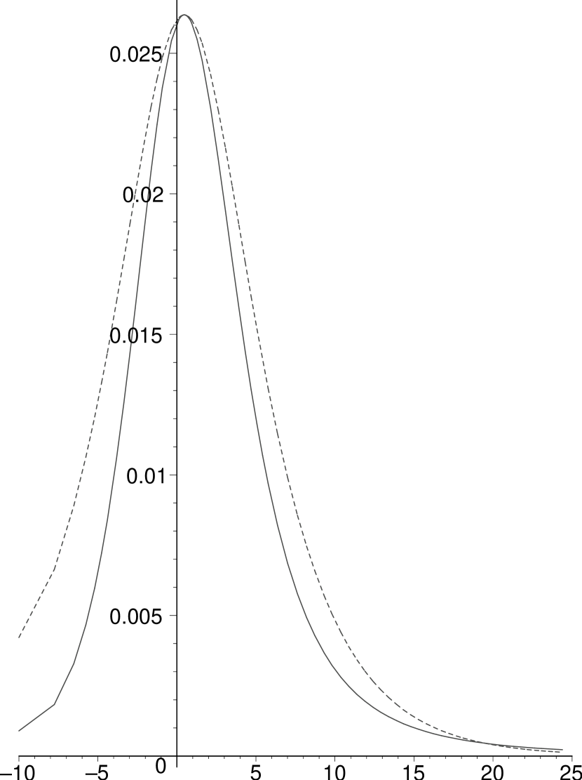
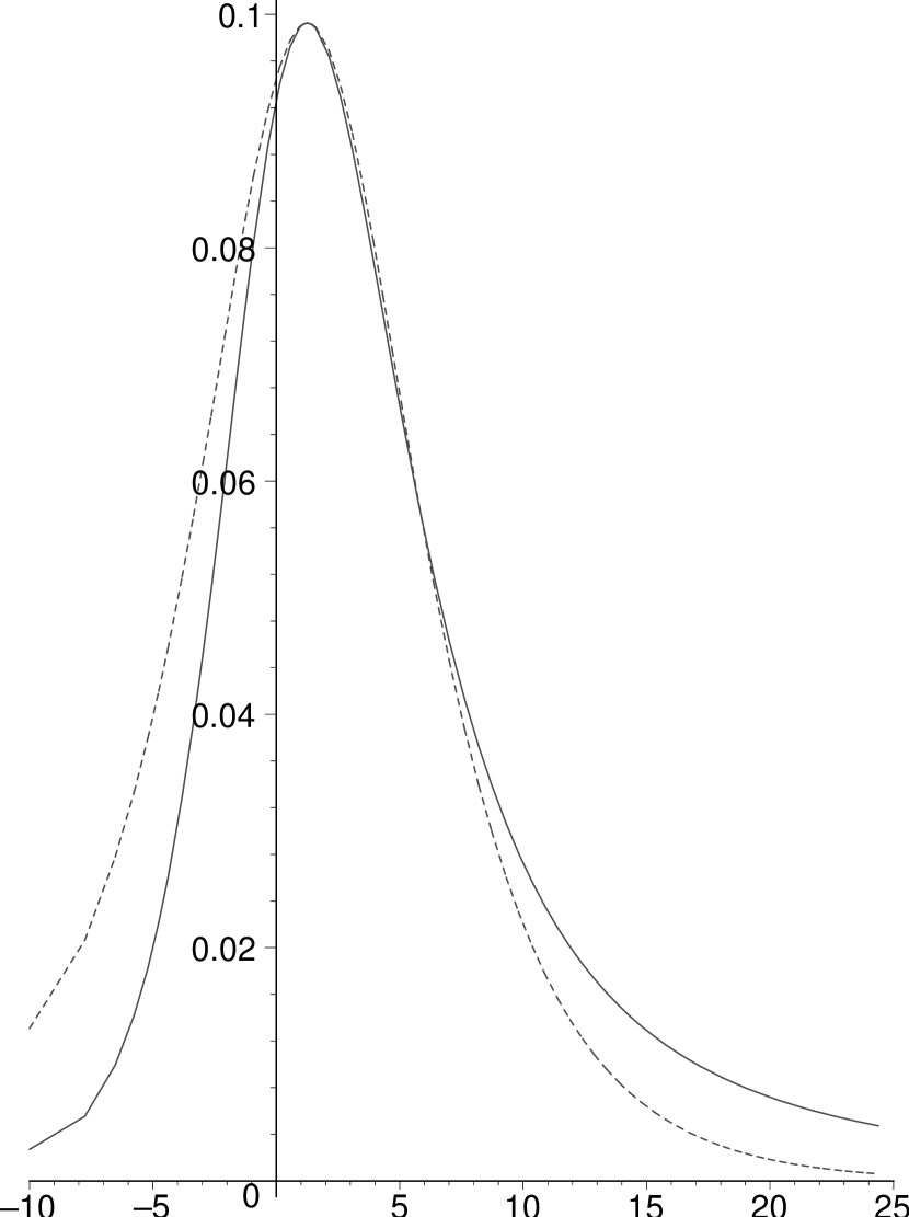
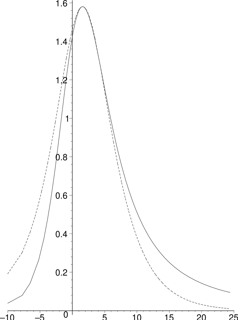
Figure 3.1: A comparison of the Regge-Wheeler potential (solid) and the Poschl-Teller potential (dotted) when the matching conditions (3.28) are used. These graphs are, from the left, for $\ell=0$, $1$ and $6$ respectively.

Before starting a discussion on surface gravity, we find some concrete results for the Schwarzschild black hole. The potential for a Schwarzschild black hole is (for a scalar field, cf (2.112))

$$V(r)=\left(1-\frac{2M}{r}\right)\left(\frac{2M}{r^{3}}+\frac{\ell(\ell+1)}{r^{2}}\right).$$ (3.29)

We find the location of the maximum:

$$\frac{{\mathrm{d}}V}{{\mathrm{d}}r} =-\frac{2}{r^{5}}(\ell(\ell+1)r^{2}+3M(1-\ell(\ell+1))r-8M^{2})=0$$ (3.30)

$$r_{0} =\frac{3[\ell(\ell+1)-1]+\sqrt{9[\ell(\ell+1)-1]^{2}+32\ell(\ell+1)}}{2\ell(\ell+1)}M.$$ (3.31)

It is now simple to find $V_{0}=V(r_{0})$, where $r_{0}$ is the location of the maximum; but such an expression is not illuminating.

To impose the second condition we need to investigate the near horizon behaviour of the potential. Introducing the tortoise coordinate (cf (2.65)):

$$\frac{{\mathrm{d}}r_{\star}}{{\mathrm{d}}r} =\frac{1}{1-2M/r}$$ (3.32)

$$r_{\star} =r-2M+2M\ln(r-2M)=x+2M\ln(x),\quad\quad x\equiv r-2M.$$ (3.33)

Near the horizon, $x$ is small. As $x\rightarrow 0$ ( or $r_{\star}\rightarrow-\infty$)

$$x\sim\exp(r_{\star}/2M).$$ (3.34)

From equation (3.29) the near horizon form of the potential is found:

$$V(x)=\frac{x}{8M^{3}}\left(1-\frac{x}{2M}\right)\bigg{(}1-\frac{3x}{2M}+\ell(\ell+1)\left[1-\frac{x}{M}\right]\bigg{)}+O\left(\frac{x^{4}}{M^{6}}\right),$$ (3.35)

or in terms of $r_{\star}$:

$$V(r_{\star})=\frac{\exp(r_{\star}/2M)}{8M^{3}}\bigg{(}\ell^{2}+\ell+1\bigg{)}+O\left(\frac{\exp(r_{\star}/M)}{M^{3}}\right).$$ (3.36)

Hence the near horizon decay rate is $1/2M$, or more formally

$$\lim_{r_{\star}\rightarrow-\infty}\frac{\ln(V(r_{\star}))}{r_{\star}}=\frac{1}{2M}.$$ (3.37)

The Poschl-Teller potential has exponential decay as one heads toward the horizon as well:

$$\lim_{r_{\star}\rightarrow-\infty}\mathcal{V}(r_{\star}) =\frac{V_{0}}{\exp(-2\alpha[r_{\star}-r_{\star}^{0}])/2}$$ (3.38)

$$=\left[2V_{0}\exp(-2\alpha r_{\star}^{0})\right]\exp(2\alpha r_{\star}).$$ (3.39)

The decay rates will agree near the horizon if and only if

$$\alpha=\frac{1}{4M}=\kappa_{h}$$ (3.40)

where $\kappa_{h}$ is the surface gravity of a Schwarzschild black hole.

Finding the QNM

Our attention is now turned to finding the QNM frequencies of the approximate Poschl-Teller potential. That is, we wish to find the QNM given

$$\frac{{\mathrm{d}}^{2}R}{{\mathrm{d}}r_{\star}^{2}}+\omega^{2}R=\frac{V_{0}}{\cosh^{2}\left(\alpha r_{\star}\right)}R,$$ (3.41)

where the $r_{\star}$ axis has been translated so that $r_{\star}^{0}=0$. The exact solution is given in terms of hypergeometric functions:

$$R(r) =C_{1}(2\cosh(2\alpha r_{\star})+2)^{1/4+G/\alpha}$$

$$\quad\times{}_{2}F_{1}\left(\frac{-2i\omega+\alpha+4G}{4\alpha},\frac{\alpha+2i\omega+4G}{4\alpha};1+\frac{4G}{2\alpha};\frac{1}{2}\cosh(2\alpha r_{\star})+\frac{1}{2}\right)$$

$$\quad+C_{2}(2\cosh(2\alpha r_{\star})+2)^{1/4-G/\alpha}$$

$$\quad\times{}_{2}F_{1}\left(\frac{2i\omega+\alpha-4G}{4\alpha},\frac{\alpha-2i\omega-4G}{4\alpha};1-\frac{4G}{2\alpha};\frac{1}{2}\cosh(2\alpha r_{\star})+\frac{1}{2}\right),$$ (3.42)

$$G =\frac{1}{4}\sqrt{\alpha^{2}-4V_{0}}.$$ (3.43)

We are wanting to look at the behaviour as $r_{\star}$ goes to infinity. The argument of the hypergeometric is dominated by the exponentially growing piece:

$$\lim_{r_{\star}\rightarrow\pm\infty}R(r)=$$

$$C_{1}\exp([\alpha+4G]|r_{\star}|/2){}_{2}F_{1}\left(\frac{\alpha-2i\omega+4G}{4\alpha},\frac{\alpha+2i\omega+4G}{4\alpha};1+\frac{4G}{2\alpha};\frac{1}{4}e^{2\alpha|r_{\star}|}\right)$$

$$+C_{2}\exp([\alpha-4G]|r_{\star}|/2){}_{2}F_{1}\left(\frac{\alpha+2i\omega-4G}{4\alpha},\frac{\alpha-2i\omega-4G}{4\alpha}];1-\frac{4G}{2\alpha};\frac{1}{4}e^{2\alpha|r_{\star}|}\right).$$ (3.44)

To express this in terms of exponential functions (and hence ingoing and outgoing waves) near infinity the following result (see equation (e.6) of [52])

$${}_{2}F_{1}(a,b;c;z) =\frac{\Gamma(c)\Gamma(b-a)}{\Gamma(b)\Gamma(c-a)}(-z)^{-a}{}_{2}F_{1}\left(a,a+1-c;a+1-b;\frac{1}{z}\right)$$

$$+\frac{\Gamma(c)\Gamma(a-b)}{\Gamma(a)\Gamma(c-b)}(-z)^{-b}{}_{2}F_{1}\left(b,b+1-c;b+1-a;\frac{1}{z}\right).$$ (3.45)

To find the asymptotic form at infinity the series expansion for the hypergeometric function is employed:

$${}_{2}F_{1}(a,b;c;z)=1+\frac{ab}{c}\frac{z}{1!}+\frac{a(a+1)b(b+1)}{c(c+1)}\frac{z^{2}}{2!}+\ldots$$ (3.46)

This allows us to replace the hypergeometric near infinity with unity. The asymptotic form of (3.42) is then (up to an irrelevant constant factor):

$$\lim_{r\rightarrow\pm\infty}R(r)\propto C_{1}\Gamma\left(1+\frac{\sqrt{\alpha^{2}-4V_{0}}}{2\alpha}\right)$$

$$\times\Bigg{[}\frac{\Gamma(i\omega/\alpha)}{\Gamma([\alpha+2i\omega+\sqrt{\alpha^{2}-4V_{0}}]/4\alpha)\Gamma([3\alpha+\sqrt{\kappa^{2}-4V_{0}}+2i\omega]/4\alpha)}e^{i\omega|r_{\star}|}$$

$$+\frac{\Gamma(-i\omega/\alpha)}{\Gamma([\alpha+\sqrt{\alpha^{2}-4V_{0}}-2i\omega]/4\alpha)\Gamma([3\alpha+\sqrt{\alpha^{2}-4V_{0}}-2i\omega]/4\alpha)}e^{-i\omega|r_{\star}|}\Bigg{]}$$

$$+C_{2}\Gamma\left(1-\frac{\sqrt{\alpha^{2}-4V_{0}}}{2\alpha}\right)$$

$$\times\Bigg{[}\frac{\Gamma(-i\omega/\alpha)}{\Gamma([\alpha-2i\omega-\sqrt{\kappa^{2}-4V_{0}}]/4\alpha)\Gamma([3\alpha-2i\omega-\sqrt{\alpha^{2}-4V_{0}}]/4\alpha)}e^{-i\omega|r_{\star}|}$$

$$+\frac{\Gamma(i\omega/\alpha)}{\Gamma([\alpha+2i\omega-\sqrt{\alpha^{2}-4V_{0}}]/4\alpha)\Gamma([3\alpha+2i\omega-\sqrt{\alpha^{2}-4V_{0}}]/4\alpha)}e^{i\omega|r_{\star}|}\Bigg{]}.$$ (3.47)

The QNM boundary condition means that the incoming waves (the part proportional to $\exp(-i\omega|r_{\star}|)$) must vanish. This implies that

$$0=\Gamma\left(-\frac{i\omega}{\alpha}\right)\Bigg{\{}C_{1}\Gamma\left(1+\frac{\sqrt{\alpha^{2}-4V_{0}}}{2\alpha}\right)$$

$$\quad\times\left[\Gamma\left(\frac{\alpha-2i\omega+\sqrt{\alpha^{2}-4V_{0}}}{4\alpha}\right)\Gamma\left(\frac{3\alpha+\sqrt{\kappa^{2}-4V_{0}}-2i\omega}{4\alpha}\right)\right]^{-1}$$

$$\quad+C_{2}\Gamma\left(1-\frac{\sqrt{\alpha^{2}-4V_{0}}}{2\alpha}\right)\times$$

$$\quad\left[\Gamma\left(\frac{\alpha-2i\omega-\sqrt{\alpha^{2}-4V_{0}}}{4\alpha}\right)\Gamma\left(\frac{3\alpha-2i\omega-\sqrt{\alpha^{2}-4V_{0}}}{4\alpha}\right)\right]^{-1}\Bigg{\}}e^{-i\omega|r_{\star}|}.$$ (3.48)

It is well known that the gamma function has no zeros in the complex plane. Candidates for QNMs then come from the fact that the Gamma function diverges at the negative integers. Specifically, letting $n$ be a positive integer, candidate QNM modes occur at

• $C_{1}=0$: Then we have one of the two remaining Gamma functions encountering a pole, i.e.:

  $$\alpha-2i\omega-\sqrt{\alpha^{2}-4V_{0}}=-4n\alpha$$ (3.49a)

  or

  $$3\alpha-2i\omega-\sqrt{\alpha^{2}-4V_{0}}=-4n\alpha$$ (3.49b)

  which implies that

  $$\omega_{n}=\sqrt{V_{0}-\left(\frac{\alpha}{2}\right)^{2}}-i\left(n+\frac{1}{2}\right)\alpha.$$ (3.49c)

• $C_{2}=0$: The only change is the sign of the square root changes.

We can finally summarise the QNM for the Poschl-Teller potential:

$$\omega_{n}=(\pm)\sqrt{V_{0}-\left(\frac{\alpha}{2}\right)^{2}}+i\left(n+\frac{1}{2}\right)\alpha.$$ (3.50)

3.2.2 Comparison of results

In comparison, the results of Ferrari and Mashhoon [25] are given by ($\ell\gg 1$)

$$\omega_{n} \approx(\pm)\frac{\ell+1/2}{3\sqrt{3}M}+i\frac{n+1/2}{3\sqrt{3}M}$$ (3.51)

$$=\frac{\alpha}{3\sqrt{3}}\left(\pm 2(2\ell+1)+i\left(n+\frac{1}{2}\right)\right).$$ (3.52)

These results are presumably given for gravitational waves, although no such statement is made by the authors (electromagnetic QNM are independent of $\ell$, and the paper focuses on gravitational and electromagnetic QNM).

It should be noted that the type of field and the angular momentum $\ell$ determine the potential completely. In particular, they determine $V_{0}$, and it follows that the real part of $\omega_{n}$ will depend on $\ell$, irrespective of the matching condition chosen.

The values of $n$ occur from the imposition of the boundary conditions on the Poschl–Teller potential. Hence the imaginary part will be evenly spaced if we match to the Poschl–Teller potential irrespective of the details of the matching conditions. The value of the spacing between the levels does depend on the matching condition. More specifically

• Matching decay rate: Real part depends on $\ell$ via $V_{0}$. The matching condition gives

  $$\alpha=\kappa_{h}$$ (3.53)

  which is independent of $\ell$, hence the imaginary spacing is constant.

• Ferrari and Mashhoon: Now $\alpha$ depends on $\ell$ as well:

  $$\alpha=\left(1-\frac{2M}{r_{0}}\right)\frac{1}{\sqrt{2V_{0}}}\sqrt{\left.\frac{{\mathrm{d}}^{2}V}{{\mathrm{d}}r}\right|_{r=r_{0}}}.$$ (3.54)

  This condition is $\ell$ dependent, so the imaginary spacing would rely on both $n$ and $\ell$. The real part has $\ell$ dependence from both $V_{0}$ and $\alpha$.

It is worth emphasising again that the imaginary spacing of the real QNMs for a given $\ell$ does not have to be constant; this is a property of the approximate Poschl–Teller potential.

$M\omega_{n}$ for a Schwarzschild black hole:
Numerical and analytic approximations 1 2 3 4 5 6 $\Im(M\omega_{s})$ 0 ?+?$i$ 0.374 + 0.089$i$ 0.599+0.093$i$ 0.809 + 0.094$i$ ? ? 0 1 ?+?$i$ 0.347 + 0.274$i$ 0.583+0.281$i$ 0.797 + 0.283$i$ ? ? 0.375 2 ?+?$i$ 0.301 + 0.478$i$ 0.552+0.479$i$ 0.772 + 0.480$i$ ? ? 0.625 3 ?+?$i$ 0.252 + 0.705$i$ 0.512+0.690$i$ 0.740 + 0.684$i$ ? ? 0.875 4 ?+?$i$ 0.208 + 0.947$i$ 0.470+0.916$i$ 0.702 + 0.898$i$ ? ? 1.125 5 ?+?$i$ 0.169 + 1.196$i$ ?+?$i$ ? ? ? 1.375 200 ?+?$i$ 0.061 + 49.860$i$ 0.078 + 49.843$i$ 0.085 + 49.837$i$ ? 0.241 + 49.397$i$ 50.125 400 ?+?$i$ 0.056 + 99.864$i$ 0.069 + 99.852$i$ 0.083 + 99.837$i$ ? 0.129 + 99.678$i$ 100.125 600 ?+?$i$ 0.054 + 149.866$i$ 0.065 + 149.856$i$ 0.078 + 149.843$i$ ? 0.0360 + 149.548$i$ 150.125 800 ?+?$i$ 0.052 + 199.867$i$ 0.062 + 199.858$i$ 0.074 + 199.847$i$ ? 0.080 + 199.817 200.125 1000 ?+?$i$ 0.051 + 249.866$i$ 0.060 + 249.860$i$ 0.072 + 249.850$i$ ? 0.086 + 249.824$i$ 250.125 3000 ?+?$i$ 0.048 + 749.871$i$ 0.053 + 749.866$i$ 0.060 + 749.860$i$ ? 0.077 + 749.844$i$ 750.125 6000 ?+?$i$ 0.0469 + 1499.872$i$ 0.051 + 1499.868$i$ 0.056 + 1499.864$i$ ? 0.068 + 1499.852$i$ 1500.125 10000 ?+?$i$ 0.0462 + 2499.873$i$ 0.049+ 2499.870$i$ 0.053 + 2499.867$i$ ? 0.063 + 2499.8571 2500.125 $\Re(M\omega_{s})$ 0.060 0.368 0.597 0.807 1.011 1.211 $\Re(M\omega_{f})$ 0.108 0.378 0.602 0.811 1.014 1.214

Table 3.1: The modes $n=0,1,2,3,4,5$ were obtained from Anderson and Glampedakis [31]. The higher modes were taken from work kindly provided by Emanuele Berti (private communication). Here $\omega_{s}$ are the frequencies by imposing (3.28c) (the “Suneeta” condition), while $\omega_{f}$ comes from imposing (3.28b) (the “Ferrari” condition). Question marks denote frequencies that I have not found numerical results for. The real parts of both Poschl-Teller approximations are independent of $n$. The imaginary part of $\omega_{s}$ is independent of $\ell$ as it is related to the surface gravity; but as $\omega_{f}$ relies on the curvature of the ($\ell$ dependent) potential the $\Im(\omega_{f})$ changes as $\ell$ does.

$M\omega_{n}$ for a Schwarzchild black hole:
Using the Mashhoon & Ferrari matching condition 1 2 3 4 5 6 100 500 $n=0$ 0.054$i$ 0.189$i$ 0.301$i$ 0.406$i$ 0.507$i$ 0.607$i$ 9.669$i$ 48.160$i$ 1 0.163$i$ 0.567$i$ 0.904$i$ 1.217$i$ 1.521$i$ 1.820$i$ 29.008$i$ 144.481$i$ 2 0.271$i$ 0.946$i$ 1.506$i$ 2.029$i$ 2.535$i$ 3.034$i$ 48.347$i$ 240.802$i$ 3 0.379$i$ 1.324$i$ 2.108$i$ 2.840$i$ 3.549$i$ 4.247$i$ 67.686$i$ 337.123 4 0.488$i$ 1.702$i$ 2.711$i$ 3.651$i$ 4.564$i$ 5.461$i$ 87.025$i$ 433.444$i$ 5 0.596$i$ 2.081$i$ 3.313$i$ 4.463$i$ 5.578$i$ 6.674$i$ 106.364$i$ 529.764$i$ 200 21.738$i$ 75.844$i$ 120.785$i$ 162.692$i$ 203.330$i$ 243.315$i$ 3877$i$ 19312$i$ 400 43.422$i$ 151.498$i$ 241.268$i$ 324.978$i$ 406.154$i$ 486.023$i$ 7745$i$ 38576$i$ 600 65.105$i$ 227.153$i$ 361.751$i$ 487.264$i$ 608.977$i$ 728.731$i$ 11612$i$ 57841$i$ 800 86.789$i$ 302.808$i$ 482.235$i$ 649.551$i$ 811.801$i$ 971.440$i$ 15481$i$ 77105$i$ 1000 108.473$i$ 378.462$i$ 602.718$i$ 811.837$i$ 1014.624$i$ 1214.148$i$ 19349$i$ 96369$i$ 3000 325.311$i$ 1135.008$i$ 1807.552$i$ 2434.699$i$ 3042.858$i$ 3641.230$i$ 58026$i$ 289011$i$ 6000 650.568$i$ 2269.827$i$ 3614.803$i$ 4868.992$i$ 6085.209$i$ 7281.853$i$ 116042$i$ 577973$i$ 10000 1084.244$i$ 3782.919$i$ 6024.471$i$ 8114.716$i$ 10141.677$i$ 12136.017$i$ 193398$i$ 963256$i$ $\Re(\omega_{n,\ell})$ 0.108 0.378 0.602 0.811 1.014 1.214 19.339 96.321

Table 3.2: This table shows the QNM calculated using Ferrari and Mashhoon’s method. The real part depends only on $\ell$, and is displayed at the bottom of the table to prevent needless duplication. At constant $\ell$ the spacing between adjacent $n$ levels is constant.

The tabulation of the QNM mode frequencies show that, at least for low values of $\ell$, the decay rate of the potential allows much more accurate modelling than matching at the peak. It should be noted that the decay toward infinity is actually polynomial, as

$$\lim_{r\rightarrow\infty}V(r)=\frac{\ell(\ell+1)}{r^{2}}$$ (3.55)

independent of the “spin”. At large $r$ there is little difference between $r$ and $r_{\star}$.

Chapter 4 Near horizon conformal field theory

When entropy was first introduced into classical physics, it was as a state function and bore no relation to “microscopic degrees of freedom” until the pioneering work of Boltzmann. It is then perhaps not completely surprising that the explanation and calculation for black hole entropy yields an answer but does not enlighten us as to the microscopic origins of black hole entropy. What is surprising is that the answer is definite; in classical physics the entropy was determined only up to an additive constant, whereas the prescription of the logarithm of the number of microstates yields an exact value. However the calculations of black hole entropy do not yield any clue to the nature, location or even existence of black hole microstates.

The black hole temperature and entropy calculations rely on very basic physics, and can easily be extended into other dimensions. This has led to the hypothesis of universality: any explanation of black hole entropy must also apply in any number of spacetime dimensions. This may seem puzzling at first – we only live in four spacetime dimensions so the fact that the calculation may not work in other dimensions seems largely irrelevant. Having the argument work in only four dimensions could actually be seen as a positive sign if there was some fundamental reason for it, as it may be an “explanation” for why the world is four dimensional. The problem is that general relativity is written in the language of differential geometry, a language that is very flexible about the dimensionality and type of manifold that it is placed on. Consequently we can take our semi-classical entropy and temperature calculations and apply them to mathematically legitimate (but presumably unphysical) black holes. Given that these same semi-classical calculations provide the only justification for us to look for microstates of black holes it would be odd if the unphysical spacetimes did not posses similar microstates; hence the universality principle. It is only a hypothesis, and it may just be (however unlikely) that quantum gravity links quantum field theory and general relativity in such a way that the only consistent theory is in four dimensions; hence in other dimensions the classical (and hence semi-classical) approximations break down. Until evidence of such a claim can be provided (or indeed suggested) by any calculation, the universality principle seems like a good guiding principle.

We also have a large number of quantum gravity candidates that are able to reproduce the correct temperature and area of a black hole such as string theory, D-branes, loop quantum gravity (LQG) and Sakharov induced gravity models. In black holes with negative cosmological constant (anti-de Sitter space or AdS) there is a correspondence with conformal field theories (CFTs) that gives the correct entropy and temperature as well. An excellent and recent review of calculations of black hole entropy that shall be used extensively throughout this chapter is Fursaev [29]. None of these models is entirely satisfactory. The LQG calculations were outlined in chapter 2, where the microstates were spin-links that penetrated the horizon. String theory calculations are often done in a spacetime that is dual to the original spacetime. As such the microstates are not even located in the right space! It is not clear that the string theory calculations can be carried out on a generic black hole; see Fursaev [29] for details. The fact that the entropy and temperature seems generic across many different theories seems to suggest one of the three possible alternatives:

• It is just a numerical coincidence. Any quantum gravity calculation that does not give the Hawking temperature or Bekenstein-Hawking entropy maybe discarded. It is just an odd curiosity that so many theories remain.

• These theories are not really different. They are the same underlying theory written in a different way, and they are formally equivalent once correct identifications are made.

• Something fundamental is being assumed in all of the models. One such suggestion is that a symmetry in the classical theory is being preserved under all these quantisations making the temperature and entropy calculations generic.

To some degree the first idea must be correct, as it is possible to concoct theories which do not give rise to the correct entropy or temperature relations (e.g. the completely indistinguishable spin-links in Polychronakos [62]). To claim that there is no reason for the existence of so many completely different theories that reproduce these results seems highly unlikely. A literal interpretation of the second idea is demonstrably false; among string theories alone many are known to be inequivalent! In the spirit of M-theory it is possible that many of the theories are different ways of writing one theory in different languages and in different limits.

This chapter is written as part of an investigation into the third possibility, that a near horizon classical conformal symmetry is preserved on quantisation and fixes the density of states and hence the entropy. This idea started when Brown and Henneaux [10] noted in classical AdS₃ that the generators of the group of diffeomorphisms at large $r$ is becomes (two copies of) the generators of CFTs, known as Virasoro algebras. Brown and Henneaux where able to conclude that any theory of quantum gravity on AdS₃ that was diffeomorphism invariant must be a conformal field theory! In two dimensions the group of conformal transformations is infinite dimensional (any homomorphic function is a conformal transformation) and the conformal symmetry is a powerful constraint; it determines the density of states up to a constant known as the central charge. In classical theories without boundaries the central charge vanishes, and hence it is normally associated with quantum theories. However Brown and Henneaux [10] showed that even classical field theories could acquire a central change if they had a boundary. In the AdS₃ calculation this boundary was taken to be the $t-\varphi$ plane at infinite radial distance. Strominger [71] showed that it was possible to obtain the Hawking-Bekenstein entropy of a negative cosmological constant black hole from the conformal field theories. In higher dimensional spaces the CFTs are finite dimensional and do not fix the density of states, and it was unclear how to perform direct generalisations. Even in three dimensions the CFT was unable to attribute individual black holes with an entropy as the CFT correspondence only applied at large $r$. I think that this problem is somewhat overstated as entropy cannot be localised; entangled particles can fly arbitrarily far apart in a “pure state” without increasing the entropy. When I allow one particle to interact with a heat bath I change the entropy of the entangled pair. Naturally one would like to be able to associate entropy with (essentially) non-interacting subsystems of the universe, but if black holes are essentially non-interacting then the asymptotic symmetry should be “essentially” obtained far enough away from each black hole that each one could be assigned an entropy. It is not a forgone conclusion that it is possible to associate entropy with individual black holes if they are strongly interacting (such as in a binary orbit). A more serious objection is that the method of using a CFT at infinity cannot distinguish between a spacetime that contains a star and a spacetime that contains a black hole.

To have a CFT account for the black hole microstates in a generic spacetime there must be a boundary, and a 2D surface on which the generators of diffeomorphisms look like (multiple copies of) Virasoro algebras. In generic black hole spacetimes one such candidate for the boundary is a horizon[14]. As the horizon has a dimensionality one lower than the spacetime any boundary conditions specified on the horizon eliminate gauge freedom there. The question of what type of horizon needs to be used is not resolved, but for the stationary case where a Killing field is available a Killing horizon is appropriate. In the stationary case the two plane spanned by the normal to the (spacelike section of the) horizon and the Killing field possess a 2D CFT as the horizon is approached[14, 70, 15, 16]. As the CFT is on the horizon, the microstates can be associated with an individual black hole. It should be emphasised that the black hole horizon is not being treated as a physical boundary, but as a convenient place to set boundary conditions that ensure the existence of a black hole (and hence in the stationary case a 2D CFT)[14]. As a consequence the “near horizon” CFTs can distinguish between stationary black holes (which posses 2D CFTs) and stationary stars (which generically do not).

Chapter 5 Near horizon stress tensors

5.1 Stationary metrics

In this chapter we investigate stationary metrics, meaning that there is an isometry of the spacetime, the orbits of which are timelike curves. We have two possibilities for a spacetime containing a black hole:

• The spacetime is static; that is the timelike (Killing) vector field is orthogonal to a family of spacelike surfaces of “constant time”. This can be shown to be equivalent to the statement that there exist coordinates in which all mixed space/time metric coefficients of the form $g_{ti}$ vanish ($i=1,2,3$). See for example Wald, page 119 [79].

• The spacetime is stationary and axisymmetric. An axisymmetric spacetime is a spacetime with an isometry that has closed spacelike curves. For a spacetime to be both stationary and axisymmetric the action of the isometries must also commute.

There is actually a third case that is less often discussed:

• The spacetime is static and non-axisymmetric. For this to occur, an ergosphere would have to exist and it could not intersect the horizon

There are no known solutions of the third type, and good reasons to suppose that they do not exist. Hawking and Ellis [41] point out that a “Penrose process” allows the existence of negative energy particles (as measured by an observer at infinity) as long as there is an ergosphere. Hawking and Ellis then argue that if the horizon and the ergosphere have no point in common then the negative energy particles cannot pass through the event horizon but must remain in the ergosphere. If it was possible to continue this process indefinitely we could mine an infinite amount of energy from the black hole. The ergosphere is constrained from spontaneously vanishing, as we require a place for the negative energy particles. The other possibility is that the event horizon and the ergosphere eventually touch, allowing particles to escape from the ergosphere into the singularity. Once there are no negative energy particles the ergosphere can be reduced to zero, as any negative energy particles can be forced into the black hole.

The above arguments come from §9.3 of Hawking and Ellis, but do not completely preclude the idea that the ergosphere is disconnected from the event horizon. For example, the Penrose process could be limited by the gravitational effects of the numerous test particles fired in to extract energy! There is a stronger statement by Hajicek [36] that insists that the ergosphere and event horizon must coincide. Hajicek’s result requires the mild technical assumption that the orbits of the timelike Killing field are complete.

Once we have discarded the possibility that the ergosphere and the event horizon do not intersect, we have to then show that a non-axisymmetric metric does not exist.

5.2 The ADM decomposition

The Arnowitt–Deser–Misner (ADM) decomposition [4] is the process of breaking a four–dimensional spacetime into a time dependent three–dimensional geometry. To do this the spacetime (or a region of the spacetime) is foliated with three dimensional spacelike surfaces, labelled by a continuous parameter $t$. The idea is that the surface $\Sigma_{t}$ represents the geometry of space at “time” $t$. There is no natural way of doing this even in special relativity, as even if one observer sees two spatially separated events as simultaneous other observers do not necessarily agree! The decomposition of spacetime into space and time (or more precisely, a series of spacelike surfaces labelled by a parameter $t$) is thus highly non-unique. For obvious reasons the ADM decomposition is also referred to as a $(3+1)$ decomposition. While there are many references available on the ADM decomposition, such as the living review article [21] or [4], I have found an elementary treatment lacking. Thus the work in this section is meant to be clarifying and does not contain any new results.

What do points on different surfaces $\Sigma_{t_{1}}$ and $\Sigma_{t_{2}}$ have to do with one another? By introducing a timelike vector field $\tau^{a}$ representing the “flow of time” we are able to identify points on $\Sigma_{t_{1}}$ with $\Sigma_{t_{2}}$ by insisting that if two points are on the same orbit as $\tau^{a}$ then they are the same point (see figure 5.2). Instead of thinking of spacetime as a foliation of spacelike hypersurfaces we can instead consider space to be the surface $\Sigma_{0}$ with a time dependent metric. Notice that the vector field $\tau^{a}$ is highly non-unique, and different choices lead to different decompositions.

To actually carry out the ADM decomposition we need to make three (non-canonical) choices:

• An initial surface $\Sigma_{0}$, representing time zero.

• A time function $t:M\rightarrow\Re$ that assigns a time to each point in the spacetime. To be consistent with the interpretation of $\Sigma_{0}$ we require that $\forall p\in\Sigma_{0}:t(p)=0$.

• A flow of time $\tau^{a}$.

A change in any of these will lead to a different decomposition of the same spacetime. Notice that the choices are not all independent or arbitrary. For example, the time function $t$ is constrained so that the surfaces of constant $t$ (i.e. $\Sigma_{t}$) are spacelike. A function $t$ that satisfies this constraint is called a valid time function. Normally the normalisation condition

$$\tau^{a}\nabla_{a}t=1$$ (5.1)

is insisted upon. I shall not insist on it, as $\tau^{a}$ becomes null as the horizon is approached.

Figure 5.1: Two figures showing the dragging of the points of $\Sigma_{0}$ along integral curves of the flow $\tau^{a}$. The time function $t$ is different on the LHS and RHS. The level surface $t=T$ (i.e. $\Sigma_{T}$) on the LHS is spacelike and well-behaved, if this occurs for all $T$ then $t$ is a valid time function. On the RHS the surface $\Sigma_{T}$ is not spacelike so $t$ is not a valid time function.

Once we have defined the time function $t$ we have a future pointing timelike vector field, $\nabla t$. Note that there is no a priori reason to pick $\tau^{a}$ so that it points in the same direction as $\nabla t$. In general, we can decompose the flow $\tau^{a}$ into a timelike normal part and a spacelike part. First, we introduce a timelike normal

$$n^{a}=g^{ab}\frac{\nabla_{b}t}{\sqrt{\left|g^{cd}(\nabla_{c}t)(\nabla_{d}t)\right|}}$$ (5.2)

and then decompose the flow of time in the following manner:

$$\tau^{a}=Nn^{a}+N^{a}$$ (5.3)

where $N$ is a scalar function called the lapse and $N^{a}$ is a spacelike vector called the shift. In an intuitive sense $N^{a}$ lies in $\Sigma_{t}$. Of course, this cannot be taken literally as $n^{a}$ and $N^{a}$ both lie in the tangent space of a point in $M$, not in $M$ itself which is where $\Sigma_{t}$ is defined! However, this intuitive idea is captured by the orthogonality requirement of the normal and the shift:

$$N^{a}n_{a}=0.$$ (5.4)

Figure 5.2 shows this decomposition. Getting the lapse is easy, as one only needs to find the component of $\tau^{a}$ along $n^{a}$:

$$N=-\tau^{a}n_{a},$$ (5.5)

or by using the normalisation condition (5.1)

$$N=+\frac{1}{\sqrt{\left|g^{cd}(\nabla_{c}t)(\nabla_{d}t)\right|}}.$$ (5.6)

The shift can be obtained by a rearrangement of (5.3). However, it is nicer to introduce a projector that will allow us to find the component of an arbitrary vector $s^{a}$ orthogonal to $n^{a}$. First we note that the component of $s^{a}$ parallel to $n^{a}$ is

$$s^{a}_{\textrm{along n}}=-n_{a}s^{a}$$ (5.7a)

and hence the orthogonal component is

$$s^{a}_{\bot\textrm{to n}}=s^{a}-s^{a}_{\textrm{along n}}n^{a}=s^{a}+n_{b}s^{b}n^{a}.$$ (5.7b)

Finally we note the identity

$$s^{a}=g^{a}{}_{b}s^{b}$$ (5.7c)

and hence

$$s^{a}_{\bot\textrm{to n}}=\left(g^{a}{}_{b}+n^{a}n_{b}\right)s^{b}.$$ (5.7d)

The quantity in brackets projects an arbitrary vector to the spacelike surface orthogonal to $$n^{a}$$, so we define

$$h^{a}{}_{b}=g^{a}{}_{b}+n^{a}n_{b}.$$ (5.7e)

In particular, we can apply the projector to the flow vector field to obtain the shift:

$$N^{a}=h^{ab}\tau_{b}.$$ (5.8)

Figure 5.2: The decomposition of $\tau^{a}$ into the shift and lapse. Picture inspired by Wald [79].

Now we give some insight into the meaning of the shift, lapse and projector. Let us consider a timelike observer moving along an integral curve of $n^{a}$. The distance measured by such an observer is given by

$${\mathrm{d}}s^{2}=-N^{2}{\mathrm{d}}t^{2}.$$ (5.9)

Using $\lambda$ as the proper time of such an observer we have

$${\mathrm{d}}t=\frac{{\mathrm{d}}\lambda}{N}.$$ (5.10)

Thus a small lapse means that a observers travelling along integral curves of $n^{a}$ (“normal observers”) experience a small “lapse” in time between two constant time surfaces. For example, if $t$ is the Killing time coordinate it takes an infinite amount of Killing time to cross an event horizon, while the proper time of a “stationary” observer slows as the horizon is approached. When using Killing time as the time function we then when an event horizon exists we have $N=0$.

Note: There is an error in the paper reproduced in Appendix G and the published version. We strongly imply that the statements “the horizon”, “$N=0$” and “infinite red-shift surface” can be used interchangeably. This is not the case: the ergosphere is an infinite redshift surface (with respect to Killing time) but has no special causal properties.

What is the interpretation for the shift? Let $(t=x^{0},x^{1},x^{2},x^{3})$ be the coordinates in a patch of the four dimensional manifold $M$. Let $(y^{1},y^{2},y^{3})$ be the three coordinates on a patch of $\Sigma_{t}$. Now consider $\Sigma_{t}$ and $\Sigma_{t+{\mathrm{d}}t}$. By construction, we are identifying the point $y\in\Sigma_{t}$ with the point in $\Sigma_{t+{\mathrm{d}}t}$ if they lie on the same integral curve of $\tau^{a}$. In fact, we can see the stronger statement

$${\mathrm{d}}y^{a}={\mathrm{d}}x^{a}-N^{a}{\mathrm{d}}t.$$ (5.11)

With a coordinate change, we can find the metric in terms of the coordinates $(t=y^{0},y^{1},y^{2},y^{3})$. We have

$${\mathrm{d}}s^{2}=g_{ab}\,{\mathrm{d}}x^{a}\,{\mathrm{d}}x^{b}=g_{ab}\,{\mathrm{d}}y^{a}\,{\mathrm{d}}y^{b}$$ (5.12)

or, in terms of the $y$ coordinate system

$${\mathrm{d}}s^{2}=g_{tt}\,{\mathrm{d}}t^{2}+2g_{ti}{\mathrm{d}}t\,({\mathrm{d}}y^{i}+N^{i}{\mathrm{d}}t)+g_{ij}({\mathrm{d}}y^{i}+N^{i}{\mathrm{d}}t)({\mathrm{d}}y^{j}+N^{j}{\mathrm{d}}t)$$ (5.13)

where $i$ and $j$ run over spacelike indices only. But the second term is zero, as the $t$ direction is orthogonal to the spacelike directions by construction. The last term has sums over ${\mathrm{d}}y^{a}$ and $N^{a}$, both of which are orthogonal to $n^{a}$. Thus there is no different between using $g_{ij}$ or $h_{ij}$ and we finally obtain

$${\mathrm{d}}s^{2} =g_{tt}\,{\mathrm{d}}t^{2}+h_{ij}({\mathrm{d}}y^{i}+N^{i}{\mathrm{d}}t)({\mathrm{d}}y^{j}+N^{j}{\mathrm{d}}t)$$ (5.14)

$$=\left(g_{tt}+h_{ij}N^{i}N^{j}\right){\mathrm{d}}t^{2}+2(h_{ij}N^{i}){\mathrm{d}}y^{i}\;{\mathrm{d}}t+h_{ij}{\mathrm{d}}y^{i}\;{\mathrm{d}}y^{j}.$$ (5.15)

Thus we see that the projector $h_{ab}$ is really the time dependent metric on the three dimensional geometry $\Sigma_{t}$. To identify the lapse we look again at the normal observers

$${\mathrm{d}}s^{2}=-N^{2}{\mathrm{d}}t^{2}=\left(g_{tt}+h_{ij}N^{i}N^{j}\right){\mathrm{d}}t^{2}$$ (5.16)

or that

$$g_{tt}=-(N^{2}+h_{ij}N^{i}N^{j}).$$ (5.17)

Hence we can write the metric in the terms of the shift and lapse by

$$g_{ab}=\left(\begin{array}[]{c|ccc}-(N^{2}+h_{ij}N^{i}N^{j})&&N_{i}&\\ \hline\cr&&&\\ N_{j}&&h_{ij}&\\ &&&\\ \end{array}\right).$$ (5.18)

5.2.1 Modified ADM for stationary spacetimes with horizons

A glance at eq. (G.10) would lead one to think naively that the lapse is given by $N$ and the shift by $\omega\;{\mathrm{d}}\varphi$, based on a simple comparison with the form of the metric in (5.18). It is true, but quite difficult to prove, that $N=0$ is the horizon. The difficulty stems from showing that the geodesics are trapped, rather than just having a perverse coordinate system that “shifts” close to the shifts at the speed of light.

To see this, we note that we cannot use the Killing vector $\zeta^{a}$ to generate time translations as $\zeta$ is spacelike in the vicinity of a rotating black holes horizon. In fact, this is the definition of the ergosphere! As the vector field $\zeta^{a}$ is not timelike this also implies that I cannot use the Killing time $t$ as the parameter labelling different surfaces. To distinguish the Killing coordinate $t$ and the time function I shall denote the latter by $\mathcal{T}$. There is a Killing vector field that is null on the horizon and timelike in the vicinity of the horizon, formed by a linear combination of the time translation Killing vector field $\zeta^{a}$ and the axisymmetric Killing field $\psi^{a}$:

$$\chi^{a}=\zeta^{a}+\Omega_{h}\psi^{a}.$$ (5.19)

As a linear combination of Killing vector fields, $\chi^{a}$ is also a Killing vector field. It is this Killing field that generates the horizon. The constant $\Omega_{h}$ is the rotational rate of the black hole, defined by taking the locally measured rotation

$$\omega=-\frac{g_{t\varphi}}{g_{\varphi\varphi}}$$ (5.20)

in the limit as the horizon is approached. The result that the rate of rotation is constant along the horizon is the rigidity theorem due to Carter [17].

We could use $\chi^{a}$ as our flow of time vector field, but that is not timelike at large distances. Instead, we use

$$\tau^{a}=\zeta^{a}+\omega\;\psi^{a}.$$ (5.21)

Notice that $\tau^{a}$ is not a Killing vector field. As $\omega$ is the locally measured rate of rotation, it does have the physically nice property of identifying a point on one time slice with a point on another time slice that has “drifted” along with the space. We also choose the time function so that $\tau=\nabla\mathcal{T}$. Hence the flow and the normal are pointing in the same direction and the shift vanishes. The lapse is given by

$$-N^{2} =\tau^{a}\tau_{a}=\zeta^{a}\zeta_{a}+\omega\;(\zeta^{a}\psi_{a}+\psi^{a}\zeta_{a})+\omega^{2}\psi^{a}\psi_{a}$$ (5.22)

$$=g_{tt}+2\omega\;g_{t\varphi}+\omega^{2}g_{\varphi\varphi}$$ (5.23)

$$=g_{tt}-2\frac{g_{t\varphi}^{2}}{g_{\varphi\varphi}}+\frac{g_{t\varphi}^{2}}{g_{\varphi\varphi}}=g_{tt}-\frac{g_{t\varphi}^{2}}{g_{\varphi\varphi}}$$ (5.24)

$$=g_{tt}-\omega^{2}\;g_{\varphi\varphi}.$$ (5.25)

5.3 Near horizon geometry for stationary Killing horizons

5.3.1 Metric for stationary non-static Killing horizons

In this section we finally tie together the loose threads developed in previous sections. First we use the assumption of an stationary (but not static) metric with a horizon; then from §5.1 we find the spacetime is also axisymmetric. Hence we may introduce coordinates $(t,\varphi,x_{1},x_{2})$ so that the metric functions $g_{\mu\nu}$ are independent of $t$ and $\varphi$. Then the condition that the spacetime is time reversible is imposed; that is the spacetime is invariant under the simultaneous changes

$$t\rightarrow-t,\quad\quad\quad\varphi\rightarrow-\varphi.$$ (5.26)

As the metric components themselves are independent of $t$ and $\varphi$, but the intervals are not, distances will be preserved iff

$$g_{x_{i}t}=g_{x_{i}\varphi}=0,\quad\quad i=1,2.$$ (5.27)

Conditions that ensure the existence of a time reversal symmetry are discussed in §5.3.1. Equivalently, time reversal symmetry can be assumed as a “physically reasonable condition”. Together these conditions ensure that the metric can be taken locally as

$$g_{\mu\nu}=\left(\begin{array}[]{cc|cc}g_{tt}(x_{1},x_{2})&g_{t\varphi}(x_{1},x_{2})&0&0\\ g_{\varphi t}(x_{1},x_{2})&g_{\varphi\varphi}(x_{1},x_{2})&0&0\\ \hline\cr 0&0&g_{x_{1}x_{1}}(x_{1},x_{2})&g_{x_{1}x_{2}}(x_{1},x_{2})\\ 0&0&g_{x_{2}x_{1}}(x_{1},x_{2})&g_{x_{2}x_{2}}(x_{1},x_{2})\end{array}\right)_{\mu\nu}.$$ (5.28)

As the spacetime decomposes into the direct sum of two 2-$d$ manifolds, an index convention that respects this is now adopted. Greek indices $\alpha,\beta,\ldots$ will represent a general spacetime index; that is it may take values from 0 to 3 representing the coordinates $(t,\varphi,x_{1},x_{2})$. Upper case latin indices $A,B,\ldots$ take the values 0 or 1 and represent the $t-\varphi$ submanifold. Lower case latin indices $a,b,\ldots$ take the value 2 or 3 and represent the coordinates $x_{1}$ or $x_{2}$ respectively. This convention is not used in earlier parts of this thesis. Such a convention allows us to write (5.28) in the much more compact form

$$g_{\mu\nu}=\left(\begin{array}[]{c|c}g_{AB}(x_{1},x_{2})&0\\ \hline\cr 0&g_{ab}(x_{1},x_{2})\end{array}\right)_{\mu\nu}.$$ (5.29)

The ADM-like decomposition described at the end of §5.2 is performed on the $t-\varphi$ submanifold. That is,

$$g_{tt} =-\left(N^{2}-\frac{g_{t\varphi}^{2}}{g_{\varphi\varphi}}\right)=-\left(N^{2}-\omega^{2}g_{\varphi\varphi}\right)$$ (5.30)

$$\omega \equiv-\frac{g_{t\varphi}}{g_{\varphi\varphi}}$$ (5.31)

where the horizon is located at $N=0$. The parameter $\omega$ defines how much the horizon “rotates” by as one travels along the orbits of $\chi^{a}$, the vector field that is null on the horizon. We have the earlier result that $\omega$ on the horizon is $\Omega_{h}$.

So far no use has been made of the coordinate freedom in $x_{1}$ and $x_{2}$. Near the horizon we can introduce a normal coordinate system. The coordinate $n$ measures the distance normal from the horizon, with the horizon occurring at $n=0$. The coordinate $z$ is a spacelike vector that lies on the horizon. The decomposition is then

$$g_{ab}=\left(\begin{array}[]{cc}1&0\\ 0&g_{zz}\end{array}\right)_{ab}.$$ (5.32)

Notice that the (now overused) word normal in this context means a spacelike vector that lies in the $x_{1}$–$x_{2}$ plane that is orthogonal to the horizon. For example, in the Schwarzschild geometry the radial coordinate $r$ would be a normal coordinate in this sense of the word. The full metric can now be given

$$g_{\mu\nu}=\left(\begin{array}[]{cc|cc}-(N^{2}-\omega^{2}g_{\varphi\varphi})&-\omega g_{\varphi\varphi}&0&0\\ -\omega g_{\varphi\varphi}&g_{\varphi\varphi}&0&0\\ \hline\cr 0&0&1&0\\ 0&0&0&g_{zz}\end{array}\right)_{\mu\nu}.$$ (5.33)

Note that this coordinate system only exists locally, it will fail as soon as two of the geodesics leaving the horizon in the $n$ direction intersect. As we are only interested in the near horizon results, the local construction is good enough.

5.3.2 Static metrics

If the metric is static then we no longer have the result that it is also axisymmetric. Physically this is because there is no rotation, and hence no tidal friction. As we know there that the Killing vector field is hypersurface orthogonal we have the result

$$g_{\mu\nu}=\left(\begin{array}[]{c|ccc}-N^{2}&0&0&0\\ \hline\cr 0&&&\\ 0&&h_{ij}&\\ 0&&&\end{array}\right)_{\mu\nu}.$$ (5.34)

In the neighbourhood of any point on the horizon we may decompose the coordinates into an on horizon part $(\varphi,z)$ and a normal coordinate $n$. The metric then takes the form

$$\hskip 36.98866pt\begin{array}[]{c@{\hspace{0.6cm}}c@{\hspace{0.6cm}}c@{\hspace{0.6cm}}c}t\hfil\hskip 17.07182pt&n\hfil\hskip 17.07182pt&\varphi\hfil\hskip 17.07182pt&z\\ \downarrow\hfil\hskip 17.07182pt&\downarrow\hfil\hskip 17.07182pt&\downarrow\hfil\hskip 17.07182pt&\downarrow\end{array}$$ (5.37)

$$g_{\mu\nu} =\left(\begin{array}[]{cc|cc}-N^{2}&0&0&0\\ 0&1&0&0\\ \hline\cr 0&0&g_{\varphi\varphi}&g_{z\varphi}\\ 0&0&g_{\varphi z}&g_{zz}\end{array}\right)_{\mu\nu}\begin{array}[]{l}\leftarrow t\\ \leftarrow n\\ \leftarrow\varphi\\ \leftarrow z.\end{array}$$ (5.46)

This exhausts the four coordinate choices we have available (choosing Killing time $t$, picking the normal $n$, and choosing $z$ and $\varphi$ so that $g_{nz}=g_{n\varphi}=0$). Without the introduction of more symmetries no further reduction is possible.

5.4 Out, damned singularity!

Once we have adopted appropriate coordinates (either for a static or stationary non-static spacetime) near the horizon, we can insist that the curvature scalars remain finite as the horizon is approached. Specifically, we require that

• $R^{2}$

• $R^{ab}R_{ab}$

• and $R_{abcd}R^{abcd}$

all remain finite as the horizon is approached. (Any linear combination with constant coefficients will also suffice, as a computational matter it is sometimes more convenient to use the traceless versions of the Ricci tensor and Riemann tensor). If any of these scalars becomes infinite as the horizon is approached then a genuine curvature singularity exists, as a scalar must be independent of the coordinates used. It is possible to have a directional curvature singularity, where any tetrad will have directions distorted as the singularity is approached. However, it can happen that the curvature in two or more independent directions can contribute opposite amounts to the curvature scalars, rendering the limit finite. Our finiteness condition is thus necessary but it is not sufficient.

In order to investigate the near-horizon geometry we take $n=0$ as the horizon and expand the lapse $N$ and the rotation rate $\omega$:

$$N(n,z) =\kappa_{h}(z)+\kappa_{1}(z)n+\frac{1}{2!}\kappa_{2}(z)n^{2}+\ldots$$ (5.47)

$$\omega(n,z) =\Omega_{h}+\omega_{1}(z)+\frac{1}{2!}\omega_{2}(z)n^{2}+\ldots$$ (5.48)

Naturally, $\omega$ is trivial in the case of static black holes! We have used the additional information that $n=0$, the horizon, corresponds to $N=0$ and that the rigidity theorem implies that $\omega(n=0)=\Omega_{h}$.

The rest of the details are simply a case of calculating the Ricci scalar, Ricci tensor squared and the Weyl tensor squared. I summarise the case for the stationary non-static case below. The static case is similar, and in both cases more details can be found in the appendices

5.4.1 The curvature invariants for stationary non-static horizons

The Ricci Scalar

The Ricci scalar for a stationary non-static black hole at the horizon is given by

$$R=\frac{g_{\varphi\varphi}(0,z)}{2\kappa_{h}(z)^{2}}\frac{\omega_{1}(z)^{2}}{n^{2}}+\mathcal{O}\left(\frac{1}{n}\right).$$ (5.49)

Assume:

• Non-extremal black hole: $\kappa_{h}(z)\neq 0$.

• The horizon geometry is regular: $g_{\varphi\varphi}\neq 0$ and is finite

Hence we must have $\omega_{1}(z)\equiv 0$ so that $R$ remains finite as $n\rightarrow 0$.

The traceless Ricci tensor

After using the fact that $\omega_{1}(z)=0$ we find:

$$R_{ab}R^{ab}-\frac{1}{4}R^{2} =\bigg{\{}\left(\left.\frac{{\mathrm{d}}\ln g_{zz}}{{\mathrm{d}}n}\right|_{n=0}\right)^{2}+\left(\left.\frac{{\mathrm{d}}\ln g_{\varphi\varphi}}{{\mathrm{d}}n}\right|_{n=0}\right)^{2}$$

$$+\left(\frac{4\kappa_{2}(z)}{\kappa_{h}(z)}\right)^{2}+\frac{8}{g_{zz}(0,z)\kappa_{h}(z)}\left(\left.\frac{{\mathrm{d}}\kappa_{h}}{{\mathrm{d}}z}\right|_{n=0}\right)^{2}\bigg{\}}\frac{1}{n^{2}}+\mathcal{O}\left(\frac{1}{n}\right).$$ (5.50)

As this is a sum of squares, we may conclude

• An alternative derivation of the zeroth law: the surface $\kappa_{h}$ is constant.

• The next term in the expansion of the lapse, $\kappa_{2}(z)$, vanishes.

• Both $\partial_{n}g_{zz}$ and $\partial_{n}g_{\varphi\varphi}$ vanish on the horizon.

The other constraints

We have yet to apply the constraint that the Weyl tensor squared yields a finite result, or use the $n^{-1}$ terms in the Ricci scalar and square of the traceless Ricci tensor. The six constraints found above render the square of the Weyl tensor finite at the horizon upon substitution, and also ensure the $n^{-1}$ pieces of the Ricci scalar and traceless Ricci tensor vanish as well.

5.5 Near horizon geometry

In all the stationary black hole cases, when we construct a tetrad from $(\chi,n,\varphi,\zeta)$ we have the result that the Einstein block diagonalises

$$G_{\hat{a}\hat{b}}=\left(\begin{array}[]{cc|c}G_{\hat{\chi}\hat{\chi}}&0&0\\ 0&-G_{\hat{\chi}\hat{\chi}}&0\\ \hline\cr 0&0&G_{\bot}\end{array}\right)\begin{array}[]{l}\leftarrow\chi\\ \leftarrow n\\ \leftarrow(\varphi,z)\end{array}$$ (5.51)

The exact form of the different components depends if you are looking at the static case or the stationary non-static case. However, the general form of the stress tensor remains in tact. It is at this point, and this point only, that we can invoke the Einstein equations to tell us that a Killing horizon requires that

$$\rho=-p_{n}$$ (5.52)

if $\rho$ is the energy density in the timelike direction $\hat{\chi}$. In particular, this conclusion is reached without any consideration for the energy conditions.

Chapter 6 Conclusions

With a range of problems so diverse, it is hard to think of a concise way of summarising all of them. Indeed, to a large extent I already have summarised them at the end of each section. Instead of explaining the problems again and how far through completion they are, I would like to leave with a list of things that I believe are easily do-able but have not yet been done. I am afraid that to the reader that this may read as a checklist of things to do, and that is indeed how I intend to use it. But after providing a 250+ page thesis, I hope that the reader will allow me this indulgence.

Algorithmic constructions

• I believe that looking at spherically symmetric but anisotropic stars is going to be a hard problem, and likely one of little physical relevance. While I believe that very compact objects such as quark stars or neutron stars are probably going to be very anisotropic, especially at the surface where crusts are expected to form, the assumption that they are static will almost certainly be false. Even a very slowly spinning star will have a large angular momentum, resulting in a very quickly rotating neutron star that has formed as the result of gravitational collapse.

• Finding a bound on the compactness for isotropic stars that also obeys the DEC looks like a simple problem. The goal would be to find a family of stars that get arbitrarily close to saturating the $8/9$ths bound, or to improve the bound and saturate that.

• Improving the variational changes method in the gravity profile to allow for arbitrarily large changes in the profile, so that more comparison bounds can be done. As can be seen from appendix B, many bounds were obtained by comparison with the Schwarzschild solution.

• The problems of ensuring the positivity of integrals, such as the expression for $\rho(r)$, seem too difficult. A more modest problem of finding large classes of functions $g(r)$ that ensure the energy density is positive everywhere may, however, be achievable.

Quasinormal modes

This section is somewhat depressing for two reasons. The first is that the motivation for looking at highly damped QNMs does not exist anymore, as the recent paper by Domagala and Lewandowski showed that the QNM conjecture was almost certainly false [24]. The other problem is that everything is very messy; one may consider that the adjective “dirty” could refer to finding the potentials as well as or better than to the spacetime! Finding an approach that is more intuitive or concrete would make me feel better than just going through screeds of algebra. This may, of course, be impossible. After all, the nice geometric results tend to span classes of spacetimes and tend to be existence theorems [for example, singularity theorems]. Here we really are interested in numerical answers for QNM, not existence answers to existence questions such as “are there an infinite number of QNMs for every black hole spacetime”? And as a numerical question, there is some expectation that the answer will come about from arduous working for different spacetimes. There is one avenue that seems worthwhile pursuing, namely

• Can we express the problem in a clean and separable way in the Newman-Penrose formalism? If so, can we assign a similar interpretation as in the Schwarzschild case?

The NP formalism allows separation of Reissner–Nordström, Kerr, Kerr-Newman and of course Schwarzschild. It is easier to see the relationship between the spectrum of the axial and polar cases when in the NP formalism, and indeed it provides a clear way to show that the two cases are isospectral in these examples. As we know that general dirty black hole spacetimes are not isospectral, we can ask the related question

• Is the utility of the Newman–Penrose formalism only significant if the spectra under consideration are isospectral?

A slightly different, but related question, would be

• How useful is the NP formalism in a situation where the standard massless fields are isospectral (as, excluding the scalar field, massless fields only possess two polarisations) at describing a massive field? Do all polarisations occur independently? Are all polarisations isospectral?

It would also be interesting and feasible, although algebraically tedious, to extend the potentials for the standard fields to the stationary dirty black holes used in the conformal symmetry section rather than just static and dirty black holes.

Although it is not something that I plan to spend much time on, I would be interested in at least seeing if the claims about the real part of highly damped QNM changes now that the QNM conjecture is almost certainly false. Do these analytical proofs hold up to closer scrutiny, or are physicists just as prone to the bandwagon effect as sociologists?

Conformal symmetry

There are two things that I would like to work through in more detail when it comes to the work that we have done on conformal transformations. The first is to see if I can find a different coordinate system in which both the central charge $c$ and the eigenvalue of $L_{0}$ remain finite as the horizon is approached. This would suggest that it is possible to have a well behaved CFT on the horizon, rather than having a theory which one is only allowed to answer certain questions for which well defined limits exist. To do this I would want to have a better understanding of the role that a central charge plays. Steve Carlip has suggested looking at a $(1+1)$ Dilaton black hole and looking at null sheets to see if a well defined central charge can be obtained in this toy model.

The other thing that would be interesting does not relate to the CFT, but rather simply the form of the geometry near the horizon. We have a null surface, and by hypothesis of stationarity the fields on that surface cannot evolve in time. One can imagine that even if this null surface was not a Killing horizon that the stress tensor would be constrained – after all massive particles cannot travel along a null surface! So while intuitively we may expect that on a null surface only “zero mass” fields would be able to exist, as massive “quanta” would be forced to travel at the speed of light to remain on this surface, I face two difficulties. The first is that it is difficult to express in general terms what is meant by a field with zero mass quanta in terms of allowed stress energies. At the moment I am not playing with a Lagrangian, only the locally defined stress energy tensor. The second point is slightly more problematic: the energy conditions have not been imposed anywhere! A timelike particle is still required to have a non-null four momentum, and so it is still possible that the only way to make such quanta have null momenta is to have singularities. This is an interesting problem, as it indicates that the restrictions on the stress energy we are seeing may have no bearing on the question of the existence of a CFT near a Killing horizon! Still, as an idea it is still too vague for me to use to prove anything with.

Finally, as the near-horizon question is more one of existence I would hope that a nice clean argument could be presented that gives the same result. A candidate for such a result is the bifurcate Killing horizon argument outlined in appendix G.

Appendix A Algorithmic construction of static perfect fluid spheres

Damien Martin and Matt Visser

Published as Physical Review D 69 (2004) 104028.

PACS numbers: 04.20.-q, 04.40.Dg, 95.30.Sf

Keywords: Fluid spheres; gr-qc/0306109

Appendix B Bounds on the interior geometry and pressure profile of static fluid spheres

Damien Martin and Matt Visser

Published as Classical and Quantum Gravity 20:3699-3716,2003

gr-qc/0306038

Appendix C Dirty black holes: Quasinormal modes

A.J.M. Medved, Damien Martin and Matt Visser

Published as Classical and Quantum Gravity 21:1393-1406, 2004

PACS numbers: 04.70.Dy, 03.65.Nk

Keywords: quasinormal modes, black holes, scattering amplitude, gr-qc/0310009

Appendix D Dirty black holes: Quasinormal modes for “squeezed” horizons

A.J.M. Medved, Damien Martin and Matt Visser

Published as Classical and Quantum Gravity 21:2393–2405,2004

PACS numbers: 04.70.-s, 04.30-w

Keywords: quasinormal modes, black holes, gr-qc/0310097

Appendix E A note on quasinormal modes: A tale of two treatments

A.J.M. Medved and Damien Martin

Published as General Relativity and Gravitation 37 (2005) 1529–1539

Keywords: QNMs, gr-qc/0311086

Appendix F Dirty black holes: Spacetime geometry and near-horizon symmetries

A J M Medved, Damien Martin and Matt Visser

22 February 2004

Published as Classical and Quantum Gravity 21 (2004) 3111–3126

gr-qc/0402069

Appendix G Dirty black holes: Symmetries at stationary non-static horizons

A J M Medved, Damien Martin and Matt Visser

5 March 2004

Published as Physical Review D 70 (2004) 024009

gr-qc/0403026

Bibliography

- [1] A. Alekseev, A. P. Polychronakos and M. Smedback. “On area and entropy of a black hole.” Phys. Lett., B574:296–300, 2003. hep-th/0004036.
- [2] N. Andersson. “On the asymptotic distribution of quasinormal-mode frequencies for Schwarzschild black holes.” Class. Quant. Grav., 10, 1993.
- [3] Nils Andersson and Bruce P. Jensen. “Scattering by black holes.” 2000. gr-qc/0011025.
- [4] R. Arnowitt, S. Deser and C. W. Misner. “The dynamics of general relativity.” In Witten [83], pp. 227–265. gr-qc/0405109.
- [5] Abhay Ashtekar. “Quantum geometry and gravity: Recent advances.” 2001. gr-qc/0112038.
- [6] A. Bachelot and A. Motet-Bachelot. “The resonances of a Schwarzschild black hole. (in French).” Annales Poincare Phys. Theor., 59:3–68, 1993.
- [7] C. Barceló and M. Visser. “Twilight for the energy conditions?” Int. J. Mod. Phys. D, 11:1553, 2002. [arXiv:gr-qc/0205066].
- [8] Jacob D. Bekenstein. “Black holes and entropy.” Phys. Rev., D7:2333–2346, 1973.
- [9] H. Bondi. “Massive spheres in general relativity.” Mon. Not. Roy. Astron. Soc., 282:303–317, 1964.
- [10] J. D. Brown and M. Henneaux. “Central charges in the canonical realization of asymptotic symmetries: An example from three-dimensional gravity.” Commun. Math. Phys., 104:207–226, 1986.
- [11] H. A. Buchdahl. “General relativistic fluid spheres.” Phys. Rev., 116:1027–1034, 1959.
- [12] H. A. Buchdahl. “General relativistic fluid spheres II: general inequalities for regular spheres.” Ap. J., 146:275–281, 1966.
- [13] Vitor Cardoso. “Quasinormal modes and gravitational radiation in black hole spacetimes.” 2004. gr-qc/0404093.
- [14] S. Carlip. “What we don’t know about BTZ black hole entropy.” Class. Quant. Grav., 15:3609–3625, 1998. hep-th/9806026.
- [15] S. Carlip. “Black hole entropy from horizon conformal field theory.” Nucl. Phys. Proc. Suppl., 88:10–16, 2000. gr-qc/9912118.
- [16] S. Carlip. “Near-horizon conformal symmetry and black hole entropy.” Phys. Rev. Lett., 88:241301, 2002. gr-qc/0203001.
- [17] Brandon Carter. “The general theory of the mechanical, electromagnetic and thermodynamic properties of black holes.” In Hawking and Israel [42], pp. 294–369.
- [18] S. Chandrasekhar. Principles of stellar dynamics. University of Chicago Press, 1942.
- [19] S. Chandrasekhar. The mathematical theory of black holes. Oxford university press, 1984.
- [20] D. Christodoulou. “Reversible and irreversible transforations in black hole physics.” Phys. Rev. Lett., 25:1596–1597, 1970.
- [21] Gregory B. Cook. “Initial data for numerical relativity.” Living Review Relativity, 3, no. 5, 15 December 2001.
- [22] Mirjam Cvetic and Finn Larsen. “Greybody factors for black holes in four dimensions: Particles with spin.” Phys. Rev., D57:6297–6310, 1998. hep-th/9712118.
- [23] E. D’Hoker and R. Jackiw. “Liouville field theory.” Phys. Rev., D26:3517, 1982.
- [24] Marcin Domagala and Jerzy Lewandowski. “Black hole entropy from quantum geometry.” 2004. gr-qc/0407051.
- [25] Valeria Ferrari and Bahram Mashhoon. “Oscillations of a black hole.” Physical Review Letters, 52, no. 16:1361–1364, 1984.
- [26] D. A. Forrester. “Some relativistic integral theorems.” Mon. Not. Roy. Astron. Soc., 51:149–156, 1970.
- [27] J. L. Friedman. Proceedings of the Royal Socitey of London A, 335:163–190, 1973.
- [28] Nanny Fröman and Per Olof Fröman. JWKB Approximation: Contributions to the theory. North-Holland, Amsterdam, 1965.
- [29] Dmitri V. Fursaev. “Can one understand black hole entropy without knowing much about quantum gravity?” 2004. gr-qc/0404038.
- [30] Matthias R. Gaberdiel. “An introduction to conformal field theory.” Rept. Prog. Phys., 63:607–667, 2000. hep-th/9910156.
- [31] Kostas Glampedakis and Nils Andersson. “Quick and dirty methods for studying black-hole resonances.” Class. Quant. Grav., 20:3441–3464, 2003. gr-qc/0304030.
- [32] Norman K. Glendenning. Compact Stars. Springer, second edition, 2000.
- [33] G. Gour and V. Suneeta. “Comparison of area spectra in loop quantum gravity.” 2004. gr-qc/0401110.
- [34] David J. Griffiths. Introduction to quantum mechanics. Prentice Hall, 1995.
- [35] J. Guven and N. O’Murchadha. “Bounds on 2M/R for static spherical objects.” Phys. Rev. D, 60:084020, 1999. [arXiv:gr-qc/9903067].
- [36] P. Hajicek. “Theory of particle detection in curved spacetimes.” Phys. Rev., D15:2757–2774, 1977.
- [37] A. Hanson, T. Regge and C. Teitelboim. Constrained Hamiltonian systems. Academia Nationale dei Lincei, Rome, 1976.
- [38] B. K. Harrison, K. S. Thorne, M. Wanako and J. A. Wheeler. Gravitational theory and gravitational collapse. University of Chicago Press, 1965.
- [39] J. B. Hartle. “Slowly rotating relativistic stars. 1. Equations of structure.” Astrophys. J., 150:1005, 1967.
- [40] S. W. Hawking. “Gravitational radiation from colliding black holes.” Phys. Rev. Lett., 26:1344–1346, 1971.
- [41] S. W. Hawking and G. F. R. Ellis. The large scale structure of space-time. Cambridge University Press, 1974.
- [42] S. W. Hawking and W. Israel, (Editors). General relativity: An Einstein Centenary Survey. Cambridge University Press, 1979.
- [43] Shahar Hod. “Bohr’s correspondence principle and the area spectrum of quantum black holes.” Phys. Rev. Lett., 81:4293, 1998. gr-qc/9812002.
- [44] Gary T. Horowitz and Veronika E. Hubeny. “Quasinormal modes of AdS black holes and the approach to thermal equilibrium.” Phys. Rev., D62:024027, 2000. hep-th/9909056.
- [45] J. N. Islam. “Some general relativistic inequalities for a star in hydrostatic equilibrium.” Mon. Not. Roy. Astron. Soc., 145:21–29, 1969.
- [46] J. N. Islam. “Some general relativistic inequalities for a star in hydrostatic equilibrium II.” Mon. Not. Roy. Astron. Soc., 147:377–386, 1970.
- [47] Panagiota Kanti and John March-Russell. “Calculable corrections to brane black hole decay. II: Greybody factors for spin 1/2 and 1.” Phys. Rev., D67:104019, 2003. hep-ph/0212199.
- [48] Kostas D. Kokkotas and Bernd G. Schmidt. “Quasi-normal modes of stars and black holes.” Living Rev. Rel., 2:2, 1999. gr-qc/9909058.
- [49] A. Kovetz. “Some extremal properties of massive spheres in general relativity.” Ap. J., 154:241–250, 1968.
- [50] A. Kovetz. “Minimal and maximal values of the central pressure and temperature in convectively stable stars.” Mon. Not. Roy. Astron. Soc., 144:549–560, 1969.
- [51] K. Krasnov. “Note on the area spectrum in quantum gravity.” Class. Quant. Grav., 15:L47–L53, 1998. gr-qc/9803074.
- [52] Lev Davidovich Landau and Evgenii Mikhailovich Lifshitz. Quantum mechanics: non-relativistic theory. Oxford university press, 3 edition, 1977.
- [53] E. W. Leaver. “An analytic representation for the quasi normal modes of Kerr black holes.” Proc. Roy. Soc. Lond., A402:285–298, 1985.
- [54] D. Martin and M. Visser. “Bounds on the interior geometry and pressure profile in static fluid spheres.” Class. Quant. Grav., 20:3699–3716, 2003. gr-qc/0306038.
- [55] Damien Martin and Matt Visser. “Algorithmic construction of static perfect fluid spheres.” Accepted for publication in Phys. Rev. D, 2003. gr-qc/0306109.
- [56] A. J. M. Medved, Damien Martin and Matt Visser. “Dirty black holes: Quasinormal modes.” Class. Quant. Grav., 21:1393–1406, 2004. Appendix C, gr-qc/0310009.
- [57] C. W. Misner, K. S. Thorne and J. A. Wheeler. Gravitation. W. H. Freeman, San Francisco, 1973.
- [58] M. S. Morris and K. S. Thorne. “Wormholes in spacetime and their use for interstellar travel: A tool for teaching general relativity.” Am. J. Phys., 56:395, 1988.
- [59] Lubos Motl. “An analytical computation of asymptotic Schwarzschild quasinormal frequencies.” Adv. Theor. Math. Phys., 6:1135–1162, 2003. gr-qc/0212096.
- [60] Lubos Motl and Andrew Neitzke. “Asymptotic black hole quasinormal frequencies.” Adv. Theor. Math. Phys., 7:307–330, 2003. hep-th/0301173.
- [61] H. P. Nollert. “On the determination of quasinormal modes of Schwarzschild black holes.” In *Rome 1985, Proceedings, General Relativity, Pt. A*, 759- 767.
- [62] Alexios P. Polychronakos. “Area spectrum and quasinormal modes of black holes.” Phys. Rev., D69:044010, 2004. hep-th/0304135.
- [63] Istvan Racz and Robert M. Wald. “Global extensions of space-times describing asymptotic final states of black holes.” 1995. gr-qc/9507055.
- [64] K. F. Riley, M. P. Hobson and S. J. Bence. Mathematical methods for physics and engineering. Cambridge University Press, 2001.
- [65] B. Robson, N. Visvanathan and W. S. Woolcock, (Editors). Cosmology: The physics of the universe. 1996.
- [66] Carlo Rovelli. Quantum gravity. Cambridge university press, 2004.
- [67] Carlo Rovelli and Lee Smolin. “Discreteness of area and volume in quantum gravity.” Nucl. Phys., B442:593–622, 1995. gr-qc/9411005.
- [68] Carlo Rovelli and Lee Smolin. “Spin networks and quantum gravity.” Phys. Rev., D52:5743–5759, 1995. gr-qc/9505006.
- [69] A. N. Schellekens. “Introduction to conformal field theory.” Fortsch. Phys., 44:605–705, 1996.
- [70] Sergey N. Solodukhin. “Conformal description of horizon’s states.” Phys. Lett., B454:213–222, 1999. hep-th/9812056.
- [71] Andrew Strominger. “Black hole entropy from near-horizon microstates.” JHEP, 02:009, 1998. hep-th/9712251.
- [72] K. Sundermeyer. Constrained dynamics, volume 169 of Lecture notes in physics. Springer, Berlin, 1982.
- [73] V. Suneeta. “Quasinormal modes for the SdS black hole: An analytical approximation scheme.” Phys. Rev., D68:024020, 2003. gr-qc/0303114.
- [74] M. Visser. Lorentzian Wormholes: From Einstein to Hawking. American Institute of Physics, 1995.
- [75] M. Visser. Notes on differential geometry . http://www.mcs.vuw.ac.nz/~visser/, Math 464, 2003.
- [76] Matt Visser. “Dirty black holes: Thermodynamics and horizon structure.” Phys. Rev., D46:2445–2451, 1992. hep-th/9203057.
- [77] Matt Visser. “Some general bounds for 1- scattering.” Phys. Rev., A59:427–438, 1999. quant-ph/9901030.
- [78] Matt Visser and Nicolas Yunes. “Power laws, scale invariance, and generalized Frobenius series: Applications to Newtonian and TOV stars near criticality.” Int. J. Mod. Phys., A18:3433–3468, 2003. gr-qc/0211001.
- [79] R. M. Wald. General Relativity. University of Chicago Press, 1984.
- [80] S. Weinberg. Gravitation and cosmology: principles and applications of the general theory of relativity. Wiley, New York, 1972.
- [81] D. L. Wiltshire. “An introduction to quantum cosmology.” In Robson et al. [65], pp. 473–531.
- [82] Ron Wiltshire. “Slowly rotating, compact fluid sources embedded in Kerr empty space-time.” 2003. gr-qc/0304097.
- [83] L. Witten, (Editor). Gravitation: An introduction to current research. Wiley, New York, 1962.