Detecting a stochastic background of gravitational waves
in the presence of non-Gaussian noise
A performance of generalized cross-correlation statistic

Abstract

We discuss a robust data analysis method to detect a stochastic background of gravitational waves in the presence of non-Gaussian noise. In contrast to the standard cross-correlation (SCC) statistic frequently used in the stochastic background searches, we consider a generalized cross-correlation (GCC) statistic, which is nearly optimal even in the presence of non-Gaussian noise. The detection efficiency of the GCC statistic is investigated analytically, particularly focusing on the statistical relation between the false-alarm and the false-dismissal probabilities, and the minimum detectable amplitude of gravitational-wave signals. We derive simple analytic formulas for these statistical quantities. The robustness of the GCC statistic is clarified based on these formulas, and one finds that the detection efficiency of the GCC statistic roughly corresponds to the one of the SCC statistic neglecting the contribution of non-Gaussian tails. This remarkable property is checked by performing the Monte Carlo simulations and successful agreement between analytic and simulation results was found.

I Introduction

A stochastic background of gravitational waves is expected to be very weak among various types of gravitational-wave signals. Such a tiny signal is produced by an incoherent superposition of many gravitational-wave signals coming from the irresolvable astrophysical objects and/or diffuse high-energy sources in the early universe. Up to now, various mechanisms to produce stochastic signals have been proposed and their amplitudes and spectra are estimated quantitatively (for the review see Ref. Allen (1997); Maggiore (2000)).

Despite the small amplitude of the signals, the stochastic backgrounds of gravitational waves contain valuable cosmological information about cosmic expansion history and astrophysical phenomena. Because of its weak interaction, the extremely early stage of the universe beyond the last scattering surface of the electromagnetic waves would be probed via the direct detection of inflationary gravitational-waves background. In this sense, gravitational-wave backgrounds are an ultimate cosmological tool and the direct detection of such signals will open a new subject of cosmology.

As a trade-off, detection of stochastic background is very difficult and the challenging problem. Recently, the observational bound of stochastic background has been updated by Laser Interferometer Gravitational Wave Observatory (LIGO Barish and Weiss (2003)) third scientific run Abbott et al. (2005) and the amplitude of signal is constrained to $\Omega_{\rm gw}\lesssim 8.4\times 10^{-4}$, where $\Omega_{\rm gw}$ is the energy density of gravitational wave divided by the critical energy density. While this is the most stringent constraint obtained from the laser interferometer Abbott et al. (2004), this bound is still larger than the limit inferred from the big-bang nucleosynthesis. Hence, for the direct detection of stochastic signals, a further development to increase the sensitivity is essential. To do this, one obvious approach is to construct a more sophisticated detector whose sensitivity level is only limited by the quantum noises. Next-generation of ground-based detectors, such as LIGO II and Large-scale Cryogenic Gravitational-wave Telescope (LCGT) Mio et al. (2003), will greatly improve the sensitivity that reaches or may beat the standard quantum limit. Furthermore, the space-based interferometer will be suited to prove gravitational wave backgrounds due to its lower observational band Kudoh et al. (2006). Another important direction is to explore the efficient and the robust technique of data analysis for signal detection.

In this paper, we shall treat the latter issue, particularly focusing on the signal detection in the presence of the non-Gaussian noises. When we search for the weak stochastic signals embedded in the detector noise, we have no practical way to discriminate between the detector noise and a stochastic signal by using only a single detector. To detect a stochastic signal, we must combine the two outputs at different detectors and quantify the statistical correlation between them. This cross-correlation technique is the robust statistical method that is still useful in the cases with large detector noises. The so-called standard cross correlation technique has been frequently used in the data analysis of laser interferometers. Note that the standard cross correlation statistic was derived under the assumption that both the signals and the instrumental noises obey stationary Gaussian process Christensen (1992); Flanagan (1993); Allen and Romano (1999). In practice, however, gravitational wave detectors do not have a pure Gaussian noise. Because of some uncontrolled mechanisms, most experiments exhibit a non-Gaussian tail. In the presence of non-Gaussianity, the direct application of the standard cross-correlation statistic significantly degrades the sensitivity of signal detection. A more appropriate cross-correlation statistic to reduce the influence of the non-Gaussian tails should be desirable in the data analysis of signal detection.

In Refs. Allen et al. (2002, 2003), the standard cross-correlation analysis was extended to deal with more realistic situation. They found that such a modified statistic shows a better performance compared to the standard cross-correlation statistic Allen et al. (2002). This modified statistic is called the locally optimal statistic Saleem (1988). Roughly speaking, the usual standard cross-correlation statistic uses all detector samples, while the locally optimal statistic excludes the samples of the non-Gaussian tails outside the main Gaussian part from the detector samples. As a result, the statistical noise variance in the locally optimal statistic becomes small due to the truncation of the samples of the non-Gaussian tail, so that the effective signal-to-noise ratio becomes large.

In this paper, we derive analytical formulas for the false-alarm and the false-dismissal probabilities and the minimum detectable signal amplitude to quantify the performance of the locally optimal statistic. Then, we demonstrate the detection efficiency of locally optimal statistic in a simple non-Gaussian noise model, in which the probability distribution of the instrumental noise is described by the two-component Gaussian noise. Based on the analytical formulas, the efficiency of the locally optimal statistic is quantified compared to the standard cross-correlation statistic.

The structure of this paper is as follows. In the next section, we briefly review the detection strategy for a stochastic background. We then introduce the generalized cross-correlation statistic which is nearly optimal in the presence of non-Gaussian noise. In Sec.III, particularly focusing on the two-component Gaussian model as a simple model of non-Gaussian noises, we analytically estimate the false-alarm and the false-dismissal probabilities. Based on this, we obtain the analytic expression for the minimum detectable amplitude of stochastic signals. The resultant analytic formulas imply that the detection efficiency of the GCC statistic roughly corresponds to the one of the SCC statistics neglecting the contribution of non-Gaussian tails. These remarkable properties are checked and confirmed by performing the Monte Carlo simulations in Sec.IV. Finally, in Sec.V, we close the paper with a summary of results and a discussion of future prospects.

II Optimal Detection Statistic in the presence of non-Gaussian Noise

As we previously mentioned, the gravitational-wave background (GWB) signal is expected to be very week and is usually masked by the detector noises. To detect such tiny signals, it is practically impossible to detect the GWB signal from the single-detector measurement. Thus, we cross-correlate the two outputs obtained from the different detectors and seek a common signal. We denote the detector outputs by $s_{i}^{k}$ with

$$s_{i}^{k}=h_{i}^{k}+n_{i}^{k},\quad(i=1,2,~{}~{}~{}k=1,\cdots,N),$$ (1)

where $i=1,2$ labels the two detectors, and $k=1,\cdots,N$ is a time index. Here, $h_{i}^{k}$ is the gravitational-wave signal, whose amplitude is typically $\epsilon$, and $n_{i}^{k}$ is the noise in each detector. The $N\times 2$ output matrix ${\cal S}$ is made up of these outputs. Throughout this paper, we discuss the optimal detection method under the assumption of weak signal, i.e., $|h_{i}^{k}|\sim\epsilon\ll|n_{i}^{k}|$.

II.1 Detection statistic

To judge whether a gravitational signal is indeed present in detector outputs or not, the simplest approach is to use a detection statistic $\Lambda=\Lambda({\cal S})$. When $\Lambda$ exceeds a threshold $\Lambda^{\ast}$, we think that the signal is detected, and not detected otherwise. The statistic $\Lambda$, which is made up of random variables ${\cal S}$, exhibits random nature under the finite sampling and because of this, we have two types of error depending on the detection criterion $\Lambda^{\ast}$. The probabilities of these errors are often called false-alarm rate and false-dismissal rate. The probability of the false alarm is the one that we conclude to have detected a signal, but the signal is in fact absent. We denote the probability by $P_{\rm FA}[\Lambda^{\ast}]$. On the other hand, the probability of the false dismissal which we denote by $P_{\rm FD}[\Lambda^{\ast}]$ is the probability that we fail to detect a signal even though the signal is in fact present. Thus, one may say that the detection statistic is optimal only when the two errors are minimized. Neyman and Pearson showed that the likelihood ratio is the optimal decision statistic that minimizes $P_{\rm FD}$ for a given value of $P_{\rm FA}$ Neyman and Pearson (1763). The likelihood ratio is given by

$$\Lambda=\frac{p({\cal S}|\epsilon)}{p({\cal S}|0)}.$$ (2)

Here, the quantity $p({\cal S}|\epsilon)$ is the probability distribution function of the observational data set ${\cal S}$ in the presence of the signal, whose amplitude is given by $\epsilon$. We are specifically concerned with the detection of weak signals. In such a situation, regarding $\epsilon$ as a small parameter, one can expand $\Lambda$ as

$$\Lambda=1+\epsilon\Lambda_{1}+\epsilon^{2}\Lambda_{2}+O(\epsilon^{3}).$$ (3)

As long as $\epsilon$ is small, the higher-order terms of $O(\epsilon^{2})$ are neglected and the quantity $\Lambda_{1}$ approximately becomes the optimal decision statistic. This statistic is called the locally optimal statistic Allen et al. (2002). If $\Lambda_{1}$ becomes zero, then $\Lambda_{2}$ is the optimal decision statistic.

II.2 Standard and generalized cross-correlation statistics

In order to obtain some insights into the locally optimal statistic, we consider the simplest situation for the data analysis of signal detection. For any two detectors, we assume that their orientations are coincident and coaligned without any systematic noise correlation between them, so that two detectors receive the same signal, i.e., $h_{1}^{k}=h_{2}^{k}=h^{k}$. There are several missions that realize such a situation. The ongoing LIGO project has two colocated detectors in the Hanford site, although the arm length of each detector is different Barish and Weiss (2003). The LCGT detector proposed by the Japanese group also has two colocated detector sharing a common arm cavity Mio et al. (2003).

In addition to the orientation of the detectors, we further assume that each detector has a white and stationary noise. In this case, the joint probability distribution of the detector noises is given by

$$p_{n}({\cal N})=\prod_{k=1}^{N}e^{-f_{1}(s_{1}^{k}-h^{k})-f_{2}(s_{2}^{k}-h^{k})},$$ (4)

where the symbol ${\cal N}$ represents the noise contribution to the output matrix ${\cal S}$. Note that Eq.(4) reduces to a multivariate Gaussian distribution if the function $f_{i}$ becomes quadratic in its argument. Thus, the function $f_{i}$ other than the quadratic form implies the non-Gaussianity of the detector noises. As for the probability of the signal amplitude, we also assume that the signal is white, so that the probability distribution function for ${\cal H}={h^{1},....,h^{N}}$ is expressed by

$$p_{h}({\cal H})=\prod_{k=1}^{N}p_{h^{k}}(h^{k}).$$ (5)

From Eqs. (1), (4) and (5), the numerator in the likelihood ratio (2) is given by

$$p({\cal S}|\epsilon)=\int dh^{1}\,\cdots\,\int dh^{N}\,p_{h}({\cal H})\,p_{n}({\cal N}).$$ (6)

Expanding the likelihood ratio with respect to $|h^{k}|\sim\epsilon\ll 1$ around zero, we obtain the locally optimal statistic Allen et al. (2002, 2003). In the present case, $\Lambda_{1}$ in Eq. (3), which includes the linear term of the signal, vanishes because the stochastic gravitational wave is usually a zero-mean signal. Therefore, $\Lambda_{2}$ turns out to be the optimal decision statistic. $\Lambda_{2}$ is composed of second derivative terms and some quadratic of the first derivative terms with respect to $s_{i}^{k}$. We then classify these terms into single-detector statistic and two-detector statistic Allen et al. (2002). The former statistic, which is described by quantities such as $f_{i}^{{}^{\prime\prime}}$ and $(f_{i}^{{}^{\prime}})^{2}$, are only relevant in the cases when the gravitational-wave signal dominates the detector noises. The latter two-detector statistic is given by Allen et al. (2002)

$$\Lambda_{\rm GCC}\propto\frac{1}{N}\sum_{k=1}^{N}f_{1}^{\prime}(s_{1}^{k})\,f_{2}^{\prime}(s_{2}^{k}),$$ (7)

where we used the fact that the signal is white. In this paper, we especially call it generalized cross-correlation (GCC) statistic.

In what follows, for the purpose of our analytic study, we treat the non-Gaussian parameters in the function $f_{i}$ as known parameter. Furthermore, we define the counterpart of the GCC statistic in the absence of non-Gaussianity as:

$$\Lambda_{\rm SCC}\equiv\frac{1}{N}\sum_{k=1}^{N}s_{1}^{k}s_{2}^{k}\,,$$ (8)

which we call the standard cross-correlation (SCC) statistic. Strictly speaking, the decision statistics derived here are not the optimal decision statistics Allen and Romano (1999); Drasco and Flanagan (2003). For instance, in the case of the Gaussian noises with unknown variances, the optimal decision statistic differs from Eq. (8) by a factor $(\hat{\sigma}_{1}\hat{\sigma}_{2})^{-1}$, where $\hat{\sigma}_{i}$ is the square-root of the autocorrelation function for the output signals $s_{i}^{k}$, i.e., $\hat{\sigma}_{i}^{2}\equiv(1/N)\sum_{k}(s_{i}^{k})^{2}$. Nevertheless, in the large-sample limit $N\to\infty$, statistical fluctuations in the autocorrelation function become negligible relative to those in $\Lambda_{\rm SCC}$ and the autocorrelation functions can be treated as constants. Thus, in the limit $N\to\infty$, the factor $(\hat{\sigma}_{1}\hat{\sigma}_{2})^{-1}$ is irrelevant and one can identify Eq. (8) as the optimal decision statistic Drasco and Flanagan (2003). In this sense, Eq. (8) may be regarded as an nearly optimal statistic. Although it seems difficult to prove that the statistic $\Lambda_{\rm GCC}$ really approaches the (locally) optimal statistic in the large-sample limit with the non-Gaussian noises, the essential properties in the statistic $\Lambda_{\rm GCC}$ is the same as those in the optimal decision statistic derived from Bayesian treatment Allen and Romano (1999). We hope that the resultant analytic formulas for detection efficiency are also useful in the practical situation that we do not know the noise parameters a priori.

III Analytic estimation of the detection efficiency

We wish to clarify how the GCC statistic improves the detection efficiency in the presence of non-Gaussian noise in an analytic way. For this purpose, we treat the simple non-Gaussian model, in which the probability distribution of the detector noises is characterized by the two-component Gaussian distribution given by Allen et al. (2002); Creighton (1999):

$$p_{n,i}(x) = e^{-f_{i}(x)}=\frac{(1-P_{i})}{\sqrt{2\pi}\sigma_{{\rm m},i}}e^{-x^{2}/2\sigma_{{\rm m},i}^{2}}+\frac{P_{i}}{\sqrt{2\pi}\sigma_{{\rm t},i}}e^{-x^{2}/2\sigma_{{\rm t},i}^{2}}\,,\quad(i=1,2)\,.$$ (9)

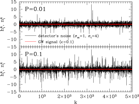
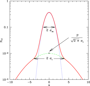
The left panel of Fig. 1 illustrates the probability distribution function of (9). This model can be characterized by the two parameters, i.e., the ratio of variance, $(\sigma_{{\rm t},i}/\sigma_{{\rm m},i})^{2}$ and the fraction of non-Gaussian tail, $P_{i}$. Here, $P_{i}$ means the total probability of the non-Gaussian tail. Of particularly interest is the case that $\sigma_{{\rm t},i}/\sigma_{{\rm m},i}>1$ and $P_{i}\ll 1$. Thus, the detector noise is approximately described by the Gaussian distribution with the main variance $\sigma_{{\rm m},i}^{2}$, but to some extent, it exhibits the non-Gaussian tail characterized by the second component of the Gaussian distribution with a large variance $\sigma_{{\rm t},i}^{2}$. The examples of this situation are illustrated in the right panel of Fig. 1.

On the other hand, we assume that the probability function of the stochastic signal is simply described by the Gaussian distribution with zero mean and with a small amplitude of the variance $\epsilon^{2}$:

$$p_{h^{k}}(h^{k})=\frac{1}{\sqrt{2\pi}\epsilon}e^{-(h^{k})^{2}/2\epsilon^{2}}.$$ (10)

Using these probability distribution functions, we derive the analytical formula for detection efficiency of the GCC statistic, i.e., $P_{\rm FA}$-$P_{\rm FD}$ curve and minimum detectable amplitude of the signal for gravitational-wave background.

Figure 1: Left: Probability distribution function of instrumental noise given by Eq.(9). The model parameters are set to $\sigma_{\rm m}=1$, $\sigma_{\rm t}=4$ and $P=0.1$. Here we dropped the detector label $i$. Right: Time-series data of the non-Gaussian noise generated by Eq. (9). Top panel shows the result with tail fraction $P=0.01$, while the bottom panel plots the case with larger value, $P=0.1$. In both panels, we specifically set the model parameters $\sigma_{\rm m}$ and $\sigma_{\rm t}$ as $\sigma_{\rm m}=1$ and $\sigma_{\rm t}=4$. For comparison, we also plot the weak signal of the stochastic gravitational waves with $\epsilon=0.1$.

III.1 $P_{\rm FA}$ versus $P_{\rm FD}$ curve

In order to quantify the detection efficiency of the GCC statistic and compare it with that of the SCC statistic, it is convenient to compute the $P_{\rm FA}$-$P_{\rm FD}$ curve. For any detection statistic $\Lambda$, the false-alarm and the false-dismissal probabilities, $P_{\rm FA}$ and $P_{\rm FD}$ are expressed as

$$P_{\rm FA}[\Lambda^{\ast}]=\int_{\Lambda^{\ast}}^{\infty}dx\,p_{\Lambda}^{(0)}(x),$$

$$P_{\rm FD}[\Lambda^{\ast}]=1-\int_{\Lambda^{\ast}}^{\infty}dx\,p_{\Lambda}^{(1)}(x).$$ (11)

Here, $p_{\Lambda}^{(0)}(x)$ and $p_{\Lambda}^{(1)}(x)$ are the probability distributions of the decision statistic in the absence and the presence of the signal, respectively. Thus, the $P_{\rm FA}$-$P_{\rm FD}$ curve is simply obtained from Eq.(11) as the parametric function of the threshold $\Lambda^{\ast}$. According to the Neyman and Pearson criterion, the best strategy to detect the stochastic signal is to choose the optimal statistic that minimizes the $P_{\rm FD}$ for a given value of $P_{\rm FA}$. In other words, if the $P_{\rm FD}$ of the GCC as function of $P_{\rm FA}$ is always smaller than that of the SCC, the GCC statistic is said to be more optimal compared to the SCC statistic.

In the large-sample limit ($N\gg 1$), the central-limit theorem would be applicable and the probabilities $p_{\Lambda}^{(0)}$ and $p_{\Lambda}^{(1)}$ can be treated as a Gaussian function. We then have

$$p_{\Lambda}^{({\cal T})}(x)=\frac{1}{\sqrt{2\pi}\Delta\Lambda^{({\cal T})}}\exp\left[-\frac{(x-\langle\Lambda^{(\cal T)}\rangle)^{2}}{2(\Delta\Lambda^{({\cal T})})^{2}}\right]\,,\quad({\cal T}=0,1)\,.$$ (12)

Here and in what follows, quantities $\langle\Lambda^{(0)}\rangle$ and $[\Delta\Lambda^{(0)}]^{2}$ denote the mean and the variance for a decision statistic in the absence of signal, while $\langle\Lambda^{(1)}\rangle$ and $[\Delta\Lambda^{(1)}]^{2}$ are the mean and the variance for a decision statistic with a signal. From Eqs. (11) and (12), the $P_{\rm FA}$-$P_{\rm FD}$ curve is given by

$$P_{\rm FD}=1-\frac{1}{2}{\rm erfc}\left[\left\{\sqrt{2}{\rm erfc}^{-1}[2P_{\rm FA}]-\frac{\langle\Lambda^{(1)}\rangle}{\Delta\Lambda^{(0)}}+\frac{\langle\Lambda^{(0)}\rangle}{\Delta\Lambda^{(0)}}\right\}\frac{1}{\sqrt{2}}\frac{\Delta\Lambda^{(0)}}{\Delta\Lambda^{(1)}}\right].$$ (13)

Here, erfc$[x]$ is the complementary error function defined by

$${\rm{erfc}}[x]=\frac{2}{\sqrt{\pi}}\int_{x}^{\infty}dz\,e^{-z^{2}}.$$ (14)

Note that in the case of the SCC statistic, the quantity $\langle\Lambda^{(1)}\rangle/\Delta\Lambda^{(0)}$ just coincides with the usual meaning of the signal-to-noise ratio (SNR). In general, the false-dismissal probability $P_{\rm FD}$ is a decreasing function of the quantity $\langle\Lambda^{(1)}\rangle/\Delta\Lambda^{(0)}$ for a given probability of false alarm $P_{\rm FA}$.

III.2 Mean and Variance for detection statistic

Next,

Our task is to calculate the means and the variances for the detection statistic, i.e., $\langle\Lambda^{({\cal T})}\rangle$ and $\left[\Delta\Lambda^{({\cal T})}\right]^{2}$. In order to compare the performance of the GCC statistic to that of the SCC statistic, we first consider the means and the variances for the SCC statistic. From Eqs. (1) and (8)-(10), the ensemble averages become

$$\langle\Lambda_{\rm SCC}^{(0)}\rangle = 0,$$ (15)

$$\left[\Delta\Lambda_{\rm SCC}^{(0)}\right]^{2} = \Big{\langle}\left[\Lambda_{\rm SCC}^{(0)}-{\big{\langle}\Lambda_{\rm SCC}^{(0)}\big{\rangle}}\right]^{2}\Big{\rangle}=\frac{\langle n_{1}^{2}\rangle\langle n_{2}^{2}\rangle}{{N}},$$ (16)

$$\langle\Lambda_{\rm SCC}^{(1)}\rangle = \epsilon^{2},$$ (17)

$$\left[\Delta\Lambda_{\rm SCC}^{(1)}\right]^{2} = \Big{\langle}\left[\Lambda_{\rm SCC}^{(1)}-\big{\langle}\Lambda_{\rm SCC}^{(1)}\big{\rangle}\right]^{2}\Big{\rangle}=\frac{1}{{N}}\left[2\langle\Lambda_{\rm SCC}^{(1)}\rangle^{2}+\langle\Lambda_{\rm SCC}^{(1)}\rangle(\langle n_{1}^{2}\rangle+\langle n_{2}^{2}\rangle)+\langle n_{1}^{2}\rangle\langle n_{2}^{2}\rangle\right],$$ (18)

where

$$\left[\Delta\Lambda_{\rm SCC}^{({\cal T})}\right]^{2}\equiv\Big{\langle}\left[\Lambda_{\rm SCC}^{({\cal T})}-\big{\langle}\Lambda_{\rm SCC}^{({\cal T})}\big{\rangle}\right]^{2}\Big{\rangle}\quad{\rm and}\quad\langle n_{i}^{2}\rangle=(1-P_{i})\sigma_{{\rm m},i}^{2}+P_{i}\sigma_{{\rm t},i}^{2}\,.\,$$ (19)

Next, we calculate the means and the variances for the GCC statistic (7). For the non-Gaussian model (9) of the instrumental noises, the derivative $f_{i}^{\prime}(x)$ in Eq. (7) is given by

$$f_{i}^{\prime}(x)=\frac{x}{\sigma_{{\rm m},i}^{2}}\left[\frac{(1-P_{i})+P_{i}(\sigma_{{\rm m},i}/\sigma_{{\rm t},i})^{3}e^{x^{2}(\sigma_{{\rm m},i}^{-2}-{\sigma_{{\rm t},i}^{-2}})/2}}{(1-P_{i})+P_{i}(\sigma_{{\rm m},i}/\sigma_{{\rm t},i})e^{x^{2}(\sigma_{{\rm m},i}^{-2}-\sigma_{{\rm t},i}^{-2})/2}}\right].$$ (20)

The expression (20) seems rather intractable to further develop the analytical calculation. However, in the situations we are interested in, i.e., $\sigma_{{\rm t},i}/\sigma_{{\rm m},i}>1$ and $P_{i}\ll 1$, the above function simply behaves like $f_{i}^{\prime}(x)\approx x/\sigma_{{\rm m},i}^{2}$ for small value of $|x|$ and $f_{i}^{\prime}(x)\approx x/\sigma_{{\rm t},i}^{2}$ for large value of $|x|$. Thus, one may apply the two-step approximation to the function (20) as:

$$f_{i}^{\prime}(s_{i}^{k})\equiv\begin{cases}\quad s_{i}^{k}&\text{$;\lvert s_{i}^{k}\rvert\leq\lvert x_{{\rm cr},i}\rvert$\,,}\\ \left(\frac{\sigma_{{\rm m},i}}{\sigma_{{\rm t},i}}\right)^{2}\,s_{i}^{k}&\text{$;\lvert s_{i}^{k}\rvert>\lvert x_{{\rm cr},i}\rvert$}\,.\end{cases}$$ (21)

Here, the quantity $x_{{\rm cr},i}$ is the critical value that characterizes the boundary between small $\lvert s_{i}^{k}\rvert$ and large $\lvert s_{i}^{k}\rvert$. Note that we adjust the overall factor of the function $f_{i}^{\prime}(s_{i}^{k})$ so as to coincide with the SCC statistic (8) in the limit $\lvert x_{{\rm cr},i}\rvert\rightarrow\infty$.

Figure 2: Derivative of the function $f(x)$ in the two-component Gaussian noise model. Left panel shows the dependence of the tail fraction $P_{i}$ keeping the ratio of noise variance fixed, i.e., $\sigma_{{\rm t},i}/\sigma_{{\rm m},i}=4$. On the other hand, right panel presents the dependence of the ratio $\sigma_{{\rm t},i}/\sigma_{{\rm m},i}$ keeping the tail fraction fixed, i.e., $P_{i}=0.1$.

Fig. 2 shows the dependence of the function $f^{\prime}(x)$ on the model parameters $P_{i}$ (left) and $\sigma_{{\rm t},i}/\sigma_{{\rm m},i}$ (right). As decreasing the tail fraction or increasing the ratio $\sigma_{{\rm t},i}/\sigma_{{\rm m},i}$, the asymptotic behavior of $f^{\prime}(x)$ steeply changes from $x/\sigma_{{\rm m},i}^{2}$ to $x/\sigma_{{\rm t},i}^{2}$ around the inflection point of $f^{\prime}(x)$. Hence, it seems reasonable to set the critical value $x_{{\rm cr},i}$ to the inflection point of $f^{\prime}(x)$. Then, the quantity $x_{{\rm cr},i}$ is approximately expressed as

$$x_{{\rm cr},i}^{2}\approx\frac{\sigma_{{\rm m},i}^{2}\sigma_{{\rm t},i}^{2}}{\sigma_{{\rm t},i}^{2}-\sigma_{{\rm m},i}^{2}}\left(\sqrt{12+\left(\log\left[\frac{P_{i}}{1-P_{i}}\frac{\sigma_{{\rm m},i}}{\sigma_{{\rm t},i}}\right]\right)^{2}}-\log\left[\frac{P_{i}}{1-P_{i}}\frac{\sigma_{{\rm m},i}}{\sigma_{{\rm t},i}}\right]\right).$$ (22)

Here, we only considered the solution satisfying the condition $(x_{{\rm cr},i}/\sigma_{{\rm m},i})>1$.

Adopting the critical value Eq. (22), with a help of two-step approximation, the means and the variances of the GCC statistic can be analytically calculated. The details of the calculation are presented in Appendix A. The resultant expressions become

$$\langle\Lambda_{\rm GCC}^{(0)}\rangle = 0\,,$$ (23)

$$\Delta\Lambda_{\rm GCC}^{(0)} = \frac{1}{\sqrt{N}}[\langle n_{1}^{2}\rangle_{\rm G}\langle n_{2}^{2}\rangle_{\rm G}]^{1/2}\,,$$ (24)

$$\langle\Lambda_{\rm GCC}^{(1)}\rangle = \{1-(P_{1}+P_{2})\}\,P_{\rm G}[x_{{\rm cr},1},\sigma_{{\rm m},1}]\,P_{\rm G}[x_{{\rm cr},2},\sigma_{{\rm m},2}]\,\epsilon^{2}\,+\,{\rm higher\,order\,terms}\,,$$ (25)

$$\Delta\Lambda_{\rm GCC}^{(1)} = \frac{1}{\sqrt{N}}\left[\langle n_{1}^{2}\rangle_{\rm G}\langle n_{2}^{2}\rangle_{\rm G}+\mathcal{O}(\epsilon^{2}\cdot\langle n_{i}^{2}\rangle_{\rm G})\right]^{1/2}\,,$$ (26)

where we defined

$$P_{{\rm G}}[x,\sigma]\equiv{\rm erf}\left[\frac{x}{\sqrt{2}\sigma}\right]-\sqrt{\frac{2}{\pi}}\frac{x}{\sigma}e^{-(x/\sigma)^{2}/2}\,,$$ (27)

$$\langle n_{i}^{2}\rangle_{\rm G} \equiv (1-P_{i})\,\sigma_{{\rm m},i}^{2}\,P_{{\rm G}}[x_{{\rm cr},i},\sigma_{{\rm m},i}]+P_{i}\,\sigma_{{\rm t},i}^{2}\,P_{{\rm G}}[x_{{\rm cr},i},\sigma_{{\rm t},i}]\,.$$ (28)

Here the quantity erf$[x]$ is the error function. In deriving Eqs.(23-26), we have neglected contributions of the integral from the region $[x_{{\rm cr},i},\infty]$. In Ref. Allen et al. (2002), this treatment is called clipping. The explicit expressions of the higher-order terms in Eq.(25) are given in Appendix A. These terms turn out to be subdominant if the non-Gaussian parameters become $P_{i}\lesssim 0.2$ or $\sigma_{{\rm t},i}/\sigma_{{\rm m},i}\gtrsim 3$. In what follows, we neglect the higher-order terms in Eq.(25) unless otherwise stated.

Now, we substitute the expressions Eqs. (22)-(26) into Eq.(13). The analytic $P_{\rm FA}$-$P_{\rm FD}$ curve for the GCC statistic is written as

$$P_{\rm FD}=1-\frac{1}{2}{\rm erfc}\left[\left\{\sqrt{2}{\rm erfc}^{-1}[2P_{\rm FA}]-\rho\left(\frac{\rho_{\rm eff}}{\rho}\right)\right\}\frac{\Delta}{\sqrt{2}}\left(\frac{\Delta_{\rm eff}}{\Delta}\right)\right],$$ (29)

where

$$\rho=\frac{\langle\Lambda_{\rm SCC}^{(1)}\rangle}{\Delta\Lambda_{\rm SCC}^{(0)}},\quad\Delta=\frac{\Delta\Lambda_{\rm SCC}^{(0)}}{\Delta\Lambda_{\rm SCC}^{(1)}},\quad\rho_{\rm eff}=\frac{\langle\Lambda_{\rm GCC}^{(1)}\rangle}{\Delta\Lambda_{\rm GCC}^{(0)}},\quad\Delta_{\rm eff}=\frac{\Delta\Lambda_{\rm GCC}^{(0)}}{\Delta\Lambda_{\rm GCC}^{(1)}}.$$ (30)

In the expression (29), we have introduced the auxiliary quantities $\rho$ and $\Delta$ to clarify the differences between the GCC and the SCC statistics. Obviously, the ratios $\rho_{\rm eff}/\rho$ and $\Delta_{\rm eff}/\Delta$ become unity when the probability distribution of noises is Gaussian, leading to the $P_{\rm FA}$-$P_{\rm FD}$ curve for SCC statistic. Thus, the deviation of these quantities from unity characterizes the efficiency of the GCC statistic.

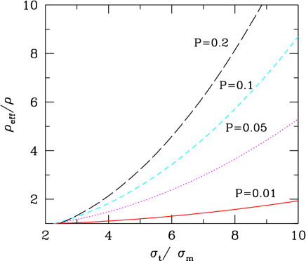
Fig. 3 shows the ratio $\rho_{\rm eff}/\rho$ as the function of $\sigma_{{\rm t}}/\sigma_{{\rm m}}$ for various tail fraction $P$. To plot the curves, just for simplicity, we assume that two detectors are identical:

$$\sigma_{\rm m}\equiv\sigma_{{\rm m},1}=\sigma_{{\rm m},2},\quad\sigma_{\rm t}\equiv\sigma_{{\rm t},1}=\sigma_{{\rm t},2},\quad P\equiv P_{1}=P_{2},\quad x_{{\rm cr}}\equiv x_{{\rm cr},1}=x_{{\rm cr},2}.$$ (31)

In Fig. 3, the ratio $\rho_{\rm eff}/\rho$ is always larger than unity for any values of $P$ and $\sigma_{\rm t}/\sigma_{\rm m}$. Recall that the quantity $\rho$ has the usual meaning of the SNR, this result implies that the clipping taken in the GCC statistic always leads to a larger effective SNR than that of the SCC statistic. On the other hand, when we evaluate the quantity $\Delta_{\rm eff}/\Delta$, one finds that this ratio is always less than $1$. These two facts indicate that the false-dismissal probability $P_{\rm FD}$ of the GCC statistic is always smaller than that of the SCC statistic. Note also that $\Delta_{\rm eff}\approx 1$ and $\Delta\approx 1$ as long as the signal $\epsilon$ is small. Thus, for a good approximation, we can set $\Delta_{\rm eff}$ to unity. Hence, the performance of the GCC statistic is mainly attributed to the ratio $\rho_{\rm eff}/\rho$.

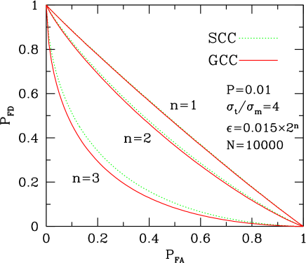
Based on this consideration, in Fig. 4, we plot the analytic $P_{\rm FA}$-$P_{\rm FD}$ curves for various signal amplitudes. Here, the parameters $P$, $\sigma_{\rm t}/\sigma_{\rm m}$ and $N$ are specifically chosen to $P=0.01$, $\sigma_{\rm t}/\sigma_{\rm m}=4$ and $N=10^{4}$. The solid and dotted lines represent the $P_{\rm FA}$-$P_{\rm FD}$ curves for the GCC and the SCC statistics, respectively. In each signal amplitude $\epsilon$, the false-dismissal probability $P_{\rm FD}$ of the GCC statistic is always smaller than that of the SCC statistic for any $P_{\rm FA}$. As expected, the performance of the GCC statistic improves as the parameter $\epsilon$ increases.

Figure 3: The quantity $\rho_{\rm eff}/\rho$ defined in Eq.(29) as function of $\sigma_{\rm t}/\sigma_{\rm m}$ in the case of the two identical detectors. From top to bottom, the tail fraction $P$ is chosen as $P=0.2$, $0.1$, $0.05$ and $0.01$.

Figure 4: Analytic $P_{\rm FA}$-$P_{\rm FD}$ curves for the standard and generalized cross-correlation statistics in the presence of the non-Gaussian noises described by the specific model (9). The sold (dashed) lines represent the $P_{\rm FA}$-$P_{\rm FD}$ curves for the GCC (SCC) statistic for the stochastic signals with amplitude $\epsilon=0.03$, $0.06$ and $0.12$ (top to bottom). Here, we assume that the two detectors are identical (see Eq. (31)). For each curves, the parameters are set as $P=0.01$, $\sigma_{\rm t}/\sigma_{\rm m}=4$ and $N=10^{4}$.

III.3 Minimum detectable amplitude

In addition to the $P_{\rm FA}$-$P_{\rm FD}$ curves, the minimum detectable amplitude of the stochastic signal, $\epsilon_{\rm detect}$ is a direct measure to quantify the performance of the detectability. In order to estimate this statistically, we must first specify the threshold values $(P_{\rm FA}^{*},~{}P_{\rm FD}^{*})$ called detection point Drasco and Flanagan (2003). For given threshold values, the minimum detectable amplitude $\epsilon_{\rm detect}$ can be uniquely determined from Eq.(29). For simplicity, we set $P_{\rm FA}^{*}$=$P_{\rm FD}^{*}$. The resultant amplitude for the GCC statistic, $\epsilon_{\rm detect}^{\rm GCC}$ is

$$\{\epsilon_{\rm detect}^{\rm GCC}\}^{2} = \frac{\displaystyle\left\{\langle n_{1}^{2}\rangle_{\rm G}\langle n_{2}^{2}\rangle_{\rm G}\right\}^{1/2}}{\displaystyle\sqrt{N}}\,\,\frac{\displaystyle 2\sqrt{2}\gamma}{\displaystyle\{1-(P_{1}+P_{2})\}\,P_{\rm G}[x_{{\rm cr},1},\sigma_{{\rm m},1}]\,P_{\rm G}[x_{{\rm cr},2},\sigma_{{\rm m},2}]},$$ (32)

$$= G^{2}(\sigma_{{\rm m},1},\sigma_{{\rm m},2},\sigma_{{\rm t},1},\sigma_{{\rm t},2},P_{1},P_{2})\,\,\{\epsilon_{\rm detect}^{\rm SCC}\}^{2}\,,$$

where we have assumed $\Delta_{\rm eff}=1$. The quantity $\gamma$ is given by $\gamma={\rm erfc}^{-1}[2P_{\rm FA}^{*}]$ and the amplitude $\epsilon_{\rm detect}^{\rm SCC}$ means the minimum detectable amplitude for the SCC statistic in the large $N$ limit Drasco and Flanagan (2003):

$$\{\epsilon_{\rm detect}^{\rm SCC}\}^{2}=\frac{2\sqrt{2}\gamma\left\{\langle n_{1}^{2}\rangle\langle n_{2}^{2}\rangle\right\}^{1/2}}{\sqrt{N}}.$$ (33)

In Eq. (32), the important quantity is the function $G$ characterizing the gain compared to the amplitude $\epsilon_{\rm detect}^{\rm SCC}$:

$$G^{2}(\sigma_{{\rm m},1},\sigma_{{\rm m},2},\sigma_{{\rm t},1},\sigma_{{\rm t},2},P_{1},P_{2})\equiv\frac{1}{\{1-(P_{1}+P_{2})\}\,P_{\rm G}[x_{{\rm cr},1},\sigma_{{\rm m},1}]\,P_{\rm G}[x_{{\rm cr},2},\sigma_{{\rm m},2}]}\left(\frac{\langle n_{1}^{2}\rangle_{\rm G}\langle n_{2}^{2}\rangle_{\rm G}}{\langle n_{1}^{2}\rangle\langle n_{2}^{2}\rangle}\right)^{\frac{1}{2}}\,.$$ (34)

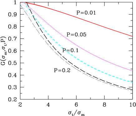
The function $G$ becomes unity when the noise probability functions reduce to the Gaussian distribution. It also approaches unity if the ratio of the noise variance $\sigma_{\rm t,i}/\sigma_{\rm m,i}$ becomes unity. For the stochastic signal $\epsilon$, we have the relation $\Omega_{\rm gw}\propto\epsilon^{2}\propto$ SNR. Thus, the minimum detectable $\Omega_{\rm gw}$ using the GCC statistic is improved by a factor $G^{2}$, compared to that of the SCC statistic.

In Fig. 5, the thick lines show the quantity $G$ as function of $\sigma_{\rm t}/\sigma_{\rm m}$ in the case of two identical detectors (see Eq. (31)). The thin lines represent the same plot, but we have taken account of the higher-order terms (44) in Appendix A. As the tail fraction becomes smaller and the ratio $\sigma_{\rm t}/\sigma_{\rm m}$ becomes larger, the thick lines tend to approach thin lines. The quantity $G$ monotonically decreases as increasing the ratio $\sigma_{\rm t}/\sigma_{\rm m}$ or the tail fraction $P$. Specifically, for the parameters $P=0.1$ and $\sigma_{\rm t}/\sigma_{\rm m}=10$, we obtain $G\sim 0.35$. This implies that the sensitivity to the stochastic signal is improved by a factor $10$ in terms of SNR, compared to the sensitivity achieved with the SCC statistic.

In the situation with $P_{i}\ll 1$ and $(\sigma_{{\rm m},i}/\sigma_{{\rm t},i})\lesssim 1$, a more compact form of the approximation for $G^{2}$ is found :

$$G^{2}\simeq\left(\frac{\langle n_{1}^{2}\rangle_{\rm G}\langle n_{2}^{2}\rangle_{\rm G}}{\langle n_{1}^{2}\rangle\langle n_{2}^{2}\rangle}\right)^{\frac{1}{2}}\simeq\prod_{i=1,2}\left[\frac{1-P_{i}}{(1-P_{i})+P_{i}\,\,(\sigma_{\rm t,i}/\sigma_{\rm m,i})^{2}}\right]^{1/2}\,.$$ (35)

Thus, when the quantity $P_{i}\,(\sigma_{\rm t,i}/\sigma_{\rm m,i})^{2}$ is larger than unity, the GCC statistic can become more powerful than the SCC statistic.

Figure 5: The function $G$ plotted against the ratio $\sigma_{\rm t}/\sigma_{\rm m}$ in the case of two identical detectors (see Eq. (31)). Here, the tail fraction $P$ is specifically chosen as $P=0.01$, $0.05$, $0.1$ and $0.2$ from top to bottom. The thick and thin lines are the function $G$ defined in Eq. (34) and the one taking account of the higher-order terms (44), respectively.

IV Monte Carlo simulation

In this section, we perform Monte Carlo simulations of the cross-correlation analysis and compare the $P_{\rm FA}$-$P_{\rm FD}$ curves and the minimum amplitude $\epsilon_{\rm detect}$ from the analytic estimates with those obtained from the numerical simulations. For the rest of this paper, we specifically assume that the two detectors are identical and satisfy the condition (31).

IV.1 Algorithm of Monte Carlo simulation

Our Monte Carlo algorithm basically follows Ref.Drasco and Flanagan (2003). We numerically calculate the false-alarm and false-dismissal probabilities $P_{\rm FA}$ and $P_{\rm FD}$ by conducting an ensemble over the $N_{\rm\scriptscriptstyle CHUNK}$ simulated experiments. For each experiment, we randomly generate two kinds of $(N\times 2)$ matrix ${\cal S}$ made up of the detector outputs, in which one output contains stochastic signals and other data contain only the instrumental noises. We then compute the decision statistic in the presence or the absence of the stochastic signals. Choosing the threshold for the decision statistic, we obtain $P_{\rm FA}$-$P_{\rm FD}$ curve. The details of the algorithm are summarized as follows (see also Ref.Drasco and Flanagan (2003)):

• Generate two kind of $(N\times 2)$ data matrix ${\cal S}$ :
  For a specific parameter set $(P,\sigma_{\rm m},\sigma_{\rm t},\epsilon,N)$, we first generate the $N$ data train which only contains the instrumental noises, i.e., $s_{i}^{k}=n_{k}^{i}$ $(i=1,2,~{}k=1,\cdots,N)$. These random data are created according to the probability distribution function (9). We then duplicate the data train and further add the stochastic signals (Eq. (10)), to the one data train, i.e., $s_{i}^{k}=h_{k}^{i}+n_{k}^{i}$ $(i=1,2,~{}k=1,\cdots,N)$.

• Compute the decision statistics $\Lambda_{\rm GCC}^{({\cal T})}$ and $\Lambda_{\rm SCC}^{({\cal T})}$ from the matrix ${\cal S}$ for ${\cal T}=0$ and $1$:
  Based on the expressions (7) and (8), under a prior knowledge of the noise parameters $(P,\sigma_{\rm m},\sigma_{\rm t})$, we compute the decision statistics $\Lambda_{\rm GCC}^{({\cal T})}$ and $\Lambda_{\rm SCC}^{({\cal T})}$ from the data matrix ${\cal S}$ in both absence and presence of the stochastic signals $({\cal T}=0,1)$. Note that the derivative $f_{i}^{\prime}(x)$ in Eq. (7) is given by Eq.(20).

• Set a threshold value $\Lambda^{\ast}$ to determine a point $(P_{\rm FA}[\Lambda^{\ast}],P_{\rm FD}[\Lambda^{\ast}])$ for GCC and SCC:
  For a given value $\Lambda^{\ast}$, we increase $P_{\rm FA}$ by the factor $1/N_{\rm\scriptscriptstyle CHUNK}$ when the condition $\Lambda^{(0)}>\Lambda^{\ast}$ is satisfied. Also, we increase $P_{\rm FD}$ by $1/N_{\rm\scriptscriptstyle CHUNK}$ if the relation $\Lambda^{(1)}<\Lambda^{*}$ holds. These operations are performed in each case of the GCC and the SCC statistics by varying the threshold value $\Lambda^{\ast}$.

• Repeat the above steps $N_{\rm\scriptscriptstyle CHUNK}$ times to estimate the probabilities $(P_{\rm FA}[\Lambda^{\ast}],P_{\rm FD}[\Lambda^{\ast}])$ for various threshold values $\Lambda^{\ast}$.

In the simulations presented below, the numbers of samples and trials are set to $N=10^{4}$ and $N_{\rm\scriptscriptstyle CHUNK}=5\times 10^{3}$, respectively. Note that the $N=10^{4}$ samples roughly correspond to the data points appropriate for the low-frequency detector like Laser Interferometer Space Antenna (LISA) Bender and et. al. (1998), for which $1$ year observation and the effective bandwidth $10^{-3}$Hz are assumed. Below, we will present the results under keeping the noise variance $\sigma_{\rm m}^{2}=1$ fixed.

IV.2 Simulation results and discussion

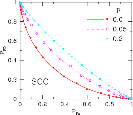
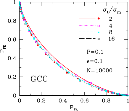
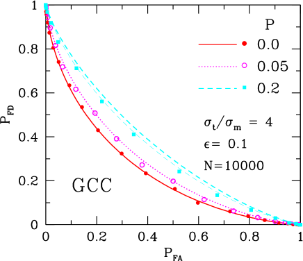
Figure 6: $P_{\rm FA}$-$P_{\rm FD}$ curves for the GCC (left) and the SCC (right) statistics. Symbols denote the simulation results, while the lines indicate the analytic prediction from Eq. (29). In each panel, the ratio of the noise variance is fixed to $\sigma_{\rm t}/\sigma_{\rm m}=4$ and the amplitude of stochastic signal is set to $\epsilon=0.1$. Note that for the tail fraction $P=0.0$, corresponding to the Gaussian noise case, the solid line and the filled circles in left panel are identical to the one in right panel: $P=0.0$(filled circles and solid); $P=0.05$ (open circles and dotted); $P=0.2$ (filled squares and dashed). The thin dashed line for $P=0.2$ indicates the analytic $P_{\rm FA}$-$P_{\rm FD}$ curve taking account of the higher-order terms (44).

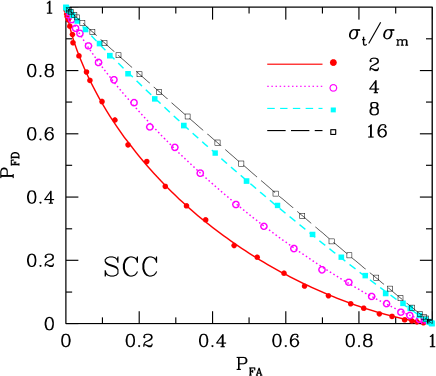
Figure 7: Same as in Fig. 6, but we here plot the dependence on the ratio $\sigma_{\rm t}/\sigma_{\rm m}$, fixing the tail fraction and the amplitude of stochastic signals to $P=0.1$ and $\epsilon=0.1$: $\sigma_{\rm t}/\sigma_{\rm m}=2$ (filled circles and solid); $\sigma_{\rm t}/\sigma_{\rm m}=4$ (open circles and dotted); $\sigma_{\rm t}/\sigma_{\rm m}=8$ (filled squares and short-dashed); $\sigma_{\rm t}/\sigma_{\rm m}=16$ (open squares and long-dashed).

Let us first show $P_{\rm FA}$-$P_{\rm FD}$ curves. In Fig. 6, the symbols denote the simulated $P_{\rm FA}$-$P_{\rm FD}$ curves for GCC (left) and SCC (right) statistics in a variety of the tail fractions $P$. Here, the signal amplitude $\epsilon=0.1$ and the ratio of the root of noise variance $\sigma_{\rm t}/\sigma_{\rm m}=4$ are kept fixed. Basically, the false-dismissal probability for a given $P_{\rm FA}$ becomes large as the tail fraction increases. However, for fixed $P$, the false-dismissal probabilities of the GCC statistic are always smaller than that of the SCC statistic. In left panel of Fig. 6, the three thick lines indicate the analytic $P_{\rm FA}$-$P_{\rm FD}$ curves without the higher-order terms in Eq.(25), which quantitatively agree with the Monte Carlo simulations. A closer look at the results for GCC statistic for the tail fraction $P=0.2$ shows a small discrepancy between analytic and simulation results, which is mainly attributed to the higher-order terms neglected in the analytic results. The thin line in left panel of Fig. 6 show the same analytic $P_{\rm FA}$-$P_{\rm FD}$ curves, but we take into account the higher-order terms (44), where the agreement becomes excellent. Note that, most of the gravitational-wave detectors have a fairly small non-Gaussian component and the analytic formulas for $P\ll 1$ without the higher-order terms would be applicable in practice.

Fig. 7 shows another plot of the $P_{\rm FA}$-$P_{\rm FD}$ curves. In each panel, fixing the tail fraction $P$ to $0.1$, the dependence on the ratio $\sigma_{\rm t}/\sigma_{\rm m}$ is depicted, in which both the analytic and the simulation results yield the similar trends. From this figure, performance of the GCC statistic seems remarkably good. Even for larger non-Gaussian tails, the $P_{\rm FA}$-$P_{\rm FD}$ curves for GCC statistic almost remain unchanged. On the other hand, the SCC statistic gets worse significantly as increasing the ratio $\sigma_{\rm t}/\sigma_{\rm m}>1$. This is indeed anticipated from the behavior of the quantity $\rho_{\rm eff}/\rho$ in Eq. (29) (see Fig. 3).

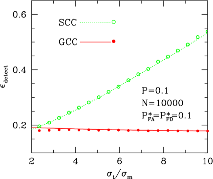
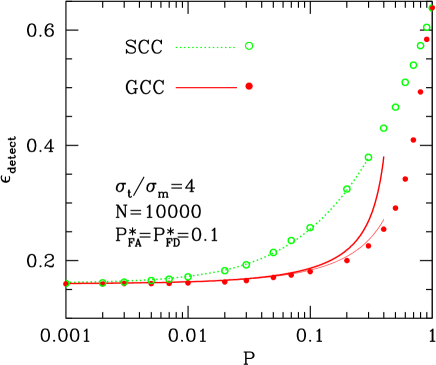
Turning to focus on the minimum detectable amplitude, we plot in Fig. 8 the dependence of the amplitude $\epsilon_{\rm detect}$ on the tail fraction $P$ (left) and the ratio of variance $\sigma_{\rm t}/\sigma_{\rm m}$ (right). In this plot, we specifically set the detection point to $(P_{\rm FA}^{\ast},\,\,P_{\rm FD}^{\ast})=(0.1,\,\,0.1)$. Note that for numerical investigation of the amplitude $\epsilon_{\rm detect}$, we ran the Monte Carlo simulation several times and vary the amplitude $\epsilon$ to find the point satisfying the condition $(P_{\rm FA},\,\,P_{\rm FD})=(0.1,\,\,0.1)$ until the accuracy with a few percentage has been achieved. In each panel, the solid and dotted lines represent the analytic estimates of the minimum amplitude for GCC and SCC statistics, respectively (Eqs. (32), (33)). The thin line in left panel shows the analytical prediction including the higher-order terms (44). For the smaller tail fraction $P\lesssim 0.1$, the analytic results for GCC statistic reasonably approximate the simulation results and the resultant amplitude $\epsilon_{\rm detect}$ is insensitive to the non-Gaussian tails. On the other hand, the minimum amplitude of SCC statistic increases in linearly proportional to the ratio of noise variance $\sigma_{\rm t}/\sigma_{\rm m}$. This remarkable feature is precisely what we expected from the analytic estimate of the minimum detectable amplitude (see Sec. III.3 and Fig. 5). That is, the dependence of the ratio $\sigma_{\rm t}/\sigma_{\rm m}$ on the functions $G$ and $\epsilon_{\rm detect}^{\rm SCC}$ almost cancels out each other, leading to the insensitivity of $\epsilon_{\rm detect}^{\rm GCC}$. Since the two-step approximation in our analytic formulas becomes a good description for a larger value $\sigma_{\rm t}/\sigma_{\rm m}$, as long as the tail fraction $P$ is small, the analytic estimation of $\epsilon_{\rm detect}^{\rm GCC}$ provides a robust and a quantitative prediction for the detection efficiency of the GCC.

Figure 8: Minimum detectable amplitude of the gravitational-wave signals as function of the tail fraction $P$ (left) and the ratio of noise variance $\sigma_{\rm t}/\sigma_{\rm m}$ (right). The ratio of noise variance in left panel is specifically chosen as $\sigma_{\rm t}/\sigma_{\rm m}=4$, while the tail fraction in right panel is set to $P=0.1$. In both panels, filled (open) circles represent the simulation results derived from the GCC (SCC) statistic. The corresponding analytic curves are also shown in solid and dotted lines based on the expressions (32) and (33). The thin line in left panel is the analytical prediction including the higher-order terms (44). Note that in these plots, detection point is specifically set to $(P_{\rm FA}^{\ast},\,P_{\rm FD}^{\ast})=(0.1,\,0.1)$ with sample points $N=10^{4}$.

V Summary

In this paper, we discussed the robust data analysis method to detect a stochastic background of gravitational wave in the presence of the non-Gaussian noise. Specifically, we have discussed the generalized cross-correlation (GCC) statistic which is a nearly optimal statistic and quantified the detection efficiency in an analytic manner. To do this, we have focused on a simple but realistic non-Gaussian noise model, i.e., two-component Gaussian noise. We derived the analytic formulas for the false-alarm and the false-dismissal probabilities as a function of threshold value $\Lambda_{\ast}$ and obtained the $P_{\rm FA}$-$P_{\rm FD}$ curves. Also, we derived the minimum detectable amplitude of stochastic signal, $\epsilon_{\rm detect}$. These analytic results are compared with the Monte Carlo simulations for the cross-correlation analysis and found that the analytic formulas provide a good description.

For small tail fraction $P_{i}\lesssim 0.1$, from Eqs. (32)–(34), minimum detectable amplitude of the stochastic signal for GCC statistic is related to that of the SCC statistic:

$$\epsilon_{\rm detect}^{\rm GCC}\simeq\left[\{1+P_{1}\,(\sigma_{{\rm t},1}/\sigma_{{\rm m},1})^{2}\}\{1+P_{2}\,(\sigma_{{\rm t},2}/\sigma_{{\rm m},2})^{2}\}\right]^{-1/4}\,\,\epsilon_{\rm detect}^{\rm SCC}$$

where the quantity $\epsilon_{\rm detect}^{\rm SCC}$ become

$$\epsilon_{\rm detect}^{\rm SCC}\simeq\left\{\frac{2\sqrt{2}\,\,\gamma}{\sqrt{N}}\,\,\sigma_{{\rm m},1}\sigma_{{\rm m},2}\right\}^{1/2}\,\,\left[\{1+P_{1}\,(\sigma_{{\rm t},1}/\sigma_{{\rm m},1})^{2}\}\{1+P_{2}\,(\sigma_{{\rm t},2}/\sigma_{{\rm m},2})^{2}\}\right]^{1/4}$$

with $\gamma$ being $\gamma=\rm{erfc}^{-1}[2P_{\rm FA}]$. Thus, these two equations indicate that the minimum amplitude of GCC statistic is mainly determined by the main part and is insensitive to the tail part of the noise probability distribution. Therefore, the quantity $\epsilon_{\rm detect}^{\rm GCC}$ is almost equivalent to the one derived from the SCC statistic just dropping the contribution of non-Gaussian tails:

$$\epsilon_{\rm detect}^{\rm GCC}\simeq\left\{\frac{2\sqrt{2}\,\,\gamma}{\sqrt{N}}\,\,\sigma_{{\rm m},1}\sigma_{{\rm m},2}\right\}^{1/2}.$$

Finally, we close this paper with comments and discussions. Throughout the paper, we have considered the two coincident and coaligned detectors with the white noise spectra. In practice, these restrictions must be relaxed. According to Refs. Allen et al. (2002, 2003), the GCC statistic has been extended to deal with a more realistic situation with non-coincident and non-co-aligned detectors of the colored noises. In this context, the analysis in the present paper roughly matches the narrow-band analysis in the Fourier domain, where the noise spectrum can be approximately described by a white noise. The extension of the present analysis to the broad-band case would be straightforward and this should deserve consideration. Another important simplification in our analysis is the stationarity of the instrumental noises and neglect of a noise correlation between two detectors. In practice, the noise correlation is known as a big obstacle in the LIGO at the Hanford site Lazzarini (2004) and it would potentially be a serious problem in the future detector, LCGT Mio et al. (2003). Thus, exploration of optimal data analysis strategy in the presence of not only the non-Gaussian noise but also the nonsteady noise and the noise correlation is very important task for future detectors.

It will be rather difficult to improve the sensitivity of the detectable amplitude by building a more sophisticated detector, due to the limitation of available technology and funds. Hence, efficient methods for data analysis such as the GCC statistic should be further exploited and it must be properly incorporated into the future detection of stochastic gravitational waves. Extending the present work to deal with a more realistic situation, we will continue to address these issues.

Appendix A Analytical expressions for the means and the variances for the GCC statistic

In this Appendix, we derive the analytical expressions (23)–(26) for the mean and the variance of the GCC statistic.

First, we compute the mean and the variance in the absence of signal, i.e., ${\cal T}=0$. Adopting the two-step approximation (21) with the critical value (22), we obtain

$$\langle\Lambda_{\rm GCC}^{(0)}\rangle = 0,$$ (36)

$$\left[\Delta\Lambda_{\rm GCC}^{(0)}\right]^{2} = \frac{\langle n_{1}^{2}\rangle_{\rm G}\langle n_{2}^{2}\rangle_{\rm G}}{{N}},$$ (37)

where

$$\langle n_{i}^{2}\rangle_{\rm G} = \int_{-x_{{\rm cr},i}}^{x_{{\rm cr},i}}dn_{i}\,\Bigl{[}n_{i}^{2}\,p_{n,i}(n_{i})\Bigr{]}+2\left(\frac{\sigma_{{\rm m},i}}{\sigma_{{\rm t},i}}\right)^{4}\int_{x_{{\rm cr},i}}^{\infty}dn_{i}\Bigl{[}n_{i}^{2}\,p_{n,i}(n_{i})\Bigr{]}.$$ (38)

In the situation we are interested in, i.e., $P_{i}\ll 1$ and $(\sigma_{{\rm m},i}/\sigma_{{\rm t},i})\lesssim 1$, the contribution of second term in the right hand side of Eq.(38) is negligibly small. Thus, the variance of noise is approximately described by the first term. In Ref. Allen et al. (2002), this effect has been called clipping. Then, we have

$$\langle n_{i}^{2}\rangle_{\rm G} \approx \int_{-x_{{\rm cr},i}}^{x_{{\rm cr},i}}dn_{i}\Bigl{[}n_{i}^{2}\,p_{n,i}(n_{i})\Bigr{]}$$ (39)

$$= (1-P_{i})\,\sigma_{{\rm m},i}^{2}\,P_{{\rm G}}[x_{{\rm cr},i},\sigma_{{\rm m},i}]+P_{i}\,\sigma_{{\rm t},i}^{2}\,P_{{\rm G}}[x_{{\rm cr},i},\sigma_{{\rm t},i}]\,.$$

Here, the quantity $P_{{\rm G}}[x,\sigma]$ is defined in Eq.(27):

$$P_{{\rm G}}[x,\sigma]\equiv{\rm erf}\left[\frac{x}{\sqrt{2}\sigma}\right]-\sqrt{\frac{2}{\pi}}\frac{x}{\sigma}e^{-(x/\sigma)^{2}/2}\,.$$

Next, we consider the mean and the variance in the presence of gravitational-wave signals. The mean $\langle\Lambda_{\rm GCC}^{(1)}\rangle$ is expressed as

$$\langle\Lambda_{\rm GCC}^{(1)}\rangle = \frac{1}{N}\sum_{k=1}^{N}\int ds_{1}^{k}\,ds_{2}^{k}\,f_{1}^{\prime}(s_{1}^{k})\cdot f_{2}^{\prime}(s_{2}^{k})\,p_{s}(s_{1}^{k},s_{2}^{k})\,,$$ (40)

where $p_{s}(s_{1}^{k},s_{2}^{k})$ is the joint probability distribution function for the two detector outputs defined by

$$p_{s}(s_{1}^{k},s_{2}^{k})\equiv\int dh^{k}\,dn_{1}^{k}\,dn_{2}^{k}\,\delta(s_{1}^{k}-h^{k}-n_{1}^{k})\,\delta(s_{2}^{k}-h^{k}-n_{2}^{k})\,p_{h^{k}}(h^{k})\,p_{n,1}(n_{1}^{k})\,p_{n,2}(n_{2}^{k}).$$ (41)

As long as the two-step approximation with clipping holds, the quantity (40) up to $\mathcal{O}(\epsilon^{2})$ becomes

$$\langle\Lambda_{\rm GCC}^{(1)}\rangle\approx\langle\Lambda_{\rm GCC}^{(1)}\rangle^{({\rm\ell})}+\langle\Lambda_{\rm GCC}^{(1)}\rangle^{({\rm h})}\,,$$ (42)

where,

$$\langle\Lambda_{\rm GCC}^{(1)}\rangle^{({\rm\ell})}=\epsilon^{2}\{1-(P_{1}+P_{2})\}P_{{\rm G}}[x_{{\rm cr},1},\sigma_{{\rm m},1}]\,P_{{\rm G}}[x_{{\rm cr},2},\sigma_{{\rm m},2}]$$ (43)

and

$$\langle\Lambda_{\rm GCC}^{(1)}\rangle^{({\rm h})} = \epsilon^{2}(P_{1}\,P_{{\rm G}}[x_{{\rm cr},1},\sigma_{{\rm t},1}]\,P_{{\rm G}}[x_{{\rm cr},2},\sigma_{{\rm m},2}]+P_{2}\,P_{{\rm G}}[x_{{\rm cr},1},\sigma_{{\rm m},1}]\,P_{{\rm G}}[x_{{\rm cr},2},\sigma_{{\rm t},2}])\,$$ (44)

$$+ \epsilon^{2}P_{1}\,P_{2}\,(P_{{\rm G}}[x_{{\rm cr},1},\sigma_{{\rm m},1}]\,P_{{\rm G}}[x_{{\rm cr},2},\sigma_{{\rm m},2}]-P_{{\rm G}}[x_{{\rm cr},1},\sigma_{{\rm t},1}]\,P_{{\rm G}}[x_{{\rm cr},2},\sigma_{{\rm m},2}]$$

$$- P_{{\rm G}}[x_{{\rm cr},1},\sigma_{{\rm m},1}]\,P_{{\rm G}}[x_{{\rm cr},2},\sigma_{{\rm t},2}]+P_{{\rm G}}[x_{{\rm cr},1},\sigma_{{\rm t},1}]\,P_{{\rm G}}[x_{{\rm cr},2},\sigma_{{\rm t},2}])\,.$$

Under the situation that $P_{i}\ll 1$ and $(\sigma_{{\rm m},i}/\sigma_{{\rm t},i})\lesssim 1$, the critical value $x_{{\rm cr},i}$ defined in Eq.(22) satisfies the condition $\sigma_{{\rm m},i}\ll x_{{\rm cr},i}\ll\sigma_{{\rm t},i}$, then $P_{{\rm G}}[x_{{\rm cr},i},\sigma_{{\rm m},i}]$ and $P_{{\rm G}}[x_{{\rm cr},i},\sigma_{{\rm t},i}]$ approximately become unity and zero, respectively. Therefore, one can regard the term $\langle\Lambda_{\rm GCC}^{(1)}\rangle^{({\rm h})}$ as the negligible higher-order terms.

Finally, using the two-step approximation with clipping, the leading order result of the quantity $\Delta\Lambda_{\rm GCC}^{(1)}$ becomes

$$\Delta\Lambda_{\rm GCC}^{(1)} = \sqrt{\langle(\Lambda_{\rm GCC}^{(1)})^{2}\rangle-\langle\Lambda_{\rm GCC}^{(1)}\rangle^{2}}$$ (45)

$$\approx \frac{(\langle n_{1}^{2}\rangle_{\rm G}\langle n_{2}^{2}\rangle_{\rm G})^{1/2}}{\sqrt{N}}\left(1+\mathcal{O}\left(\frac{\epsilon^{2}}{\langle n_{i}^{2}\rangle_{\rm G}}\right)\right).$$ (46)

Thus, in the present situation that the detector noises dominate the gravitational signal, we can reasonably treat the quantity $\Delta\Lambda_{\rm GCC}^{(1)}$ as

$$\Delta\Lambda_{\rm GCC}^{(1)}\approx\frac{(\langle n_{1}^{2}\rangle_{\rm G}\langle n_{2}^{2}\rangle_{\rm G})^{1/2}}{\sqrt{N}}=\Delta\Lambda_{\rm GCC}^{(0)}\,.$$ (47)

References

• Allen (1997) B. Allen, Proceedings of the Les Houches School on Astrophysical Sources of Gravitational Waves, edited by Jean-Alain Marck and Jean-Pierre Lasota, (Cambridge University Press, Cambridge) (1997).
• Maggiore (2000) M. Maggiore, Phys. Rept. 331, 283 (2000), eprint gr-qc/9909001.
• Barish and Weiss (2003) B. Barish and R. Weiss, Phys. Today 52, 44 (2003).
• Abbott et al. (2005) B. Abbott et al. (LIGO Scientific), Phys. Rev. Lett. 95, 221101 (2005), eprint astro-ph/0507254.
• Abbott et al. (2004) B. Abbott et al. (LIGO), Phys. Rev. D69, 102001 (2004).
• Mio et al. (2003) N. Mio et al. (LCGT Collaboration), Prog. Theor. Phys. Suppl. 151, 221 (2003).
• Kudoh et al. (2006) H. Kudoh, A. Taruya, T. Hiramatsu, and Y. Himemoto, Phys. Rev. D73, 064006 (2006), eprint gr-qc/0511145.
• Christensen (1992) N. Christensen, Phys. Rev. D46, 5250 (1992).
• Flanagan (1993) E. E. Flanagan, Phys. Rev. D48, 2389 (1993), eprint astro-ph/9305029.
• Allen and Romano (1999) B. Allen and J. D. Romano, Phys. Rev. D59, 102001 (1999), eprint gr-qc/9710117.
• Allen et al. (2002) B. Allen, J. D. E. Creighton, E. E. Flanagan, and J. D. Romano, Phys. Rev. D65, 122002 (2002), eprint gr-qc/0105100.
• Allen et al. (2003) B. Allen, J. D. E. Creighton, E. E. Flanagan, and J. D. Romano, Phys. Rev. D67, 122002 (2003), eprint gr-qc/0205015.
• Saleem (1988) A. K. Saleem, Signal Detection in Non-Gaussian Noise (Springer-Verlag, New York) (1988).
• Neyman and Pearson (1763) J. Neyman and K. Pearson, Philos. Trans. R. Soc. London. 53, 370 (1763).
• Drasco and Flanagan (2003) S. Drasco and E. E. Flanagan, Phys. Rev. D67, 082003 (2003), eprint gr-qc/0210032.
• Creighton (1999) J. D. E. Creighton, Phys. Rev. D60, 021101 (1999), eprint gr-qc/9901075.
• Bender and et. al. (1998) P. L. Bender and et. al., LISA Pre-Phase A Report (1998).
• Lazzarini (2004) A. e. a. Lazzarini, Phys. Rev. D70, 062001 (2004), eprint gr-qc/0403093.