On asymptotic behavior of anisotropic Dvali-Gabadadze-Porrati branes

Abstract

The braneworld model of Dvali-Gabadadze-Porrati (DGP) provides an interesting alternative to a positive cosmological constant by modifying gravity at large distances. We investigate the asymptotic behavior of homogeneous and anisotropic cosmologies on the DGP brane. It is shown that all Bianchi models except type IX isotropize, as in general relativity, if the so called $E_{\mu\nu}$ term satisfies some energy condition. Isotropization can proceed slower in DGP gravity than in general relativity.

In recent years some attempts have been made to give an alternative to a positive cosmological constant due to a modification of gravity at large distances. These attempts are motivated by that they themselves are theoretically interesting possibilities, as well as by the cosmological observations indicating the present acceleration of the universe acc ; Bennett:2003bz . Among various realizations of a long distance modification of gravity, here we focus on the braneworld model of Dvali-Gabadadze-Porrati (DGP) Dvali:2000hr ; Dvali:2000xg ; Lue:2005ya .

The gravitational part of the action that describes the DGP braneworld is given by

$$S=\frac{1}{2\kappa_{5}^{2}}\int d^{5}x\sqrt{-g^{(5)}}R^{(5)}+\frac{1}{2\kappa^{2}}\int d^{4}x\sqrt{-g}R,$$ (1)

where $g^{(5)}$ is the five-dimensional bulk metric and $g$ is the four-dimensional induced metric on the brane. The length scale

$$r_{0}:=\frac{\kappa_{5}^{2}}{2\kappa^{2}}$$ (2)

plays a crucial role in this model. Assuming spatial homogeneity and isotropy, the modified Friedmann equation on the brane is obtained as Deffayet:2000uy ; Deffayet:2001pu

$$H^{2}=\frac{\kappa^{2}}{3}\rho+\frac{1}{2r_{0}^{2}}\pm\frac{1}{2r_{0}^{2}}\sqrt{1+\frac{4}{3}r_{0}^{2}\kappa^{2}\rho}.$$ (3)

Thus (in the ‘$+$’ branch) the DGP brane admits the self-accelerating solution at late times without introducing a cosmological constant:

$$H\to\frac{1}{r_{0}}.$$ (4)

In the framework of general relativity, Wald showed that initially expanding homogeneous cosmological models (Bianchi models) isotropize in the presence of a positive cosmological constant $\Lambda$ Wald:1983ky . The trace of the extrinsic curvature $K$ of the homogeneous hypersufaces is shown to be “squeezed,”

$$\frac{3}{\alpha}\leq K\leq\frac{1}{\alpha}F_{{\rm GR}}(t),$$ (5)

where $\alpha:=\sqrt{3/\Lambda}$ and

$$F_{{\rm GR}}(t):=\frac{3}{\tanh(t/\alpha)},$$ (6)

with $t$ being the proper time. Accordingly, one finds that the shear of the homogeneous hypersurfaces $\sigma_{ab}$ rapidly approaches zero,

$$\sigma_{ab}\sigma^{ab}\leq\frac{2}{3\alpha^{2}}\left[F^{2}_{{\rm GR}}(t)-9\right]\to 0.$$ (7)

This is the so called cosmic no hair theorem. It is interesting to see the asymptotic behavior of Bianchi models in a gravitational theory where a cosmological constant is mimicked by a modification of gravity, rather than some energy-momentum component. In the present paper we try to extend Wald’s result in DGP gravity.

Throughout the paper we take the effective four-dimensional approach Shiromizu:1999wj . Namely, we use the effective Einstein equations on the brane Maeda:2003ar which can be written as

$$\frac{G_{ab}+E_{ab}}{4r_{0}^{2}}=f_{ab},$$ (8)

where

$$f_{ab} := -\frac{1}{4}\tilde{G}_{ac}\tilde{G}_{b}^{~{}c}+\frac{1}{12}\tilde{G}\tilde{G}_{ab}+g_{ab}\left(\frac{1}{8}\tilde{G}_{cd}\tilde{G}^{cd}-\frac{1}{24}\tilde{G}^{2}\right),$$ (9)

$$\tilde{G}_{ab} := G_{ab}-\kappa^{2}T_{ab},$$ (10)

and $T_{ab}$ is the matter energy-momentum tensor. Here all the tensors live on the brane. The five-dimensional gravitational effect is encoded into $E_{ab}$ coming from the bulk Weyl tensor, which cannot be determined locally on the brane. Instead of solving the five-dimensional field equations, in the following we consider some energy condition for this Weyl term.

We assume that the matter energy-momentum tensor satisfies the dominant and strong energy conditions so that

$$T_{ab}t^{a}t^{b}\geq 0,$$ (11)

and

$$\left(T_{ab}-\frac{1}{2}g_{ab}T\right)t^{a}t^{b}\geq 0,$$ (12)

where $t^{a}$ is a timelike vector. We define

$$\zeta:=\tilde{G}_{ab}n^{a}n^{b},$$ (13)

$$Q_{a}:=-\tilde{G}_{cd}h^{c}_{~{}a}n^{d},$$ (14)

$$S_{ab}:=\tilde{G}_{cd}h^{c}_{~{}a}h^{d}_{~{}b},$$ (15)

$${\cal U}:=-\frac{1}{\kappa^{2}}E_{ab}n^{a}n^{b},$$ (16)

where $n^{a}$ is the unit normal to the homogeneous hypersurfaces and $h_{ab}=g_{ab}+n_{a}n_{b}$ is the spatial metric. We decompose $S_{ab}$ into its trace $S$ and tracefree part $\beta_{ab}$ as

$$S_{ab}=\frac{1}{3}Sh_{ab}+\beta_{ab}.$$ (17)

The initial-value constraint of the effective Einstein equations (8) is given by

$$G_{ab}n^{a}n^{b}-\kappa^{2}{\cal U}=\frac{r_{0}^{2}}{3}\zeta^{2}-\frac{r_{0}^{2}}{2}\beta_{ab}\beta^{ab}.$$ (18)

This can be rewritten in the form

$$\zeta=G_{ab}n^{a}n^{b}-\kappa^{2}T_{ab}n^{a}n^{b}=\frac{3}{2r_{0}^{2}}+\epsilon\frac{3}{2r_{0}^{2}}\sqrt{1+\frac{4}{3}r_{0}^{2}\kappa^{2}\left(T_{ab}n^{a}n^{b}-{\cal U}\right)+\frac{2r_{0}^{4}}{3}\beta_{ab}\beta^{ab}},$$ (19)

where $\epsilon=\pm 1$ and we are interested in the ‘+’ branch. Now we assume that the Weyl term ${\cal U}$ is negative or negligible, imposing the energy condition ${\cal U}\leq 0$. If ${\cal U}$ becomes positive and dominates over the other terms, the expression in the square root vanishes and the universe evolves into a singularity at a finite scale factor (as was pointed out in Ref. Maeda:2003ar for the homogeneous model).

Another equation we need is the generalized Raychaudhuri equation:

$$R_{ab}n^{a}n^{b}=\kappa^{2}{\cal U}-r_{0}^{2}Q_{a}Q^{a}+\frac{2r_{0}^{2}}{3}\zeta^{2}+\frac{r_{0}^{2}}{3}S\zeta.$$ (20)

Noting that

$$\zeta+S=2\tilde{G}_{ab}n^{a}n^{b}+g^{ab}\tilde{G}_{ab}=2R_{ab}n^{a}n^{b}-2\kappa^{2}\left(T_{ab}-\frac{1}{2}g_{ab}T\right)n^{a}n^{b},$$

we have

$$\left(1-\frac{2r_{0}^{2}}{3}\zeta\right)R_{ab}n^{a}n^{b}=\kappa^{2}{\cal U}-r_{0}^{2}Q_{a}Q^{a}+\frac{r_{0}^{2}}{3}\zeta\left[\zeta-2\kappa^{2}\left(T_{ab}-\frac{1}{2}g_{ab}T\right)n^{a}n^{b}\right].$$ (21)

Both $G_{ab}n^{a}n^{b}$ and $R_{ab}n^{a}n^{b}$ can be expressed in terms of the three-geometry of the homogeneous hypersurfaces and their extrinsic curvature $K_{ab}$. As usual, we decompose the extrinsic curvature into its trace and the shear parts,

$$K_{ab}=\frac{1}{3}Kh_{ab}+\sigma_{ab}.$$ (22)

Then we obtain

$$G_{ab}n^{a}n^{b}=\frac{1}{2}R^{(3)}+\frac{1}{3}K^{2}-\frac{1}{2}\sigma_{ab}\sigma^{ab},$$ (23)

$$R_{ab}n^{a}n^{b}=-\dot{K}-\frac{1}{3}K^{2}-\sigma_{ab}\sigma^{ab},$$ (24)

where $R^{(3)}$ is the Ricci scalar of the homogeneous hypersurface and a dot stands for a derivative with respect to the proper time $t$. It is well known that in all Bianchi models except type IX we have Wald:1983ky

$$R^{(3)}\leq 0.$$ (25)

From this fact, Eq (23), and the definition of $\zeta$ (13) we obtain an inequality $K^{2}\geq 3\zeta$. Furthermore, Eq. (19) implies that $\zeta\geq 3/r_{0}^{2}$. Thus we have

$$K^{2}\geq 3\zeta\geq\frac{9}{r_{0}^{2}}.$$ (26)

In terms of $K$ and $\sigma_{ab}$ Eq. (21) can be rewritten as

$$\dot{K}=-\frac{1}{3}K^{2}-\sigma_{ab}\sigma^{ab}+\left(\frac{2r_{0}^{2}}{3}\zeta-1\right)^{-1}\left\{\kappa^{2}{\cal U}-r_{0}^{2}Q_{a}Q^{a}+\frac{r_{0}^{2}}{3}\zeta\left[\zeta-2\kappa^{2}\left(T_{ab}-\frac{1}{2}g_{ab}T\right)n^{a}n^{b}\right]\right\}.$$ (27)

Thus we have

$$\dot{K}\leq-\frac{1}{3}K^{2}+\frac{r_{0}^{2}\zeta^{2}/3}{2r_{0}^{2}\zeta/3-1}\leq-\frac{1}{3}K^{2}\frac{K^{2}-9/r_{0}^{2}}{2K^{2}-9/r_{0}^{2}}.$$ (28)

Integrating this inequality, we obtain

$$K\leq\frac{1}{r_{0}}F(t),$$ (29)

where $F(t)$ is defined by

$$\frac{t}{r_{0}}=\frac{3}{F(t)}+\frac{1}{2}\ln\left[\frac{F(t)+3}{F(t)-3}\right].$$ (30)

The function $F(t)$ approaches $3$ at late times and hence the expansion rate $K$ approaches the constant value $3/r_{0}$. Since $K^{2}/3-\sigma_{ab}\sigma^{ab}/2\geq\zeta\geq 3/r_{0}^{2}$, we find that

$$\sigma_{ab}\sigma^{ab}\leq\frac{2}{3r_{0}^{2}}\left[F^{2}(t)-9\right].$$ (31)

Thus the shear approaches zero as $t\to 0$.

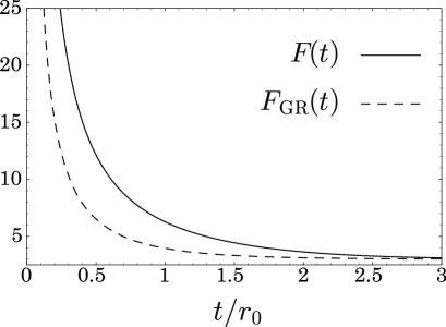
Figure 1: The functions $F(t)$ (solid curve) and $F_{{\rm GR}}(t)$ (dashed curve), which give the upper limit of the expansion rate $K$.

Now let us compare our result with the result of general relativity. The upper limit of the expansion rate in general relativity, Eq. (6), can be rewritten as

$$\frac{t}{r_{0}}=\frac{1}{2}\ln\left[\frac{F_{{\rm GR}}(t)+3}{F_{{\rm GR}}(t)-3}\right],$$ (32)

where $\alpha$ was replaced by $r_{0}$ so that we have the same value of the final expansion rate. From this and Eq. (30) we see that

$$F(t)\geq F_{{\rm GR}}(t),$$ (33)

as is shown in Fig. 1. This implies that isotropization can proceed slower in DGP gravity than in general relativity, though the time scale of isotropization is basically given by $r_{0}$ in both theories.

In summary, we have studied the asymptotic behavior of anisotropic DGP branes, on which a long distance modification of gravity leads to an effective “cosmological constant” without introducing a cosmological-constant-like energy momentum component. We have shown that all Bianchi types (except type IX) isotropize, provided that ${\cal U}\leq 0$, and isotropization can proceed slower in the DGP braneworld than in general relativity. A negative or negligible value of ${\cal U}$ is understood as a sufficient condition for isotropization. To check that the anisotropic brane metric with ${\cal U}\leq 0$ indeed leads to a consistent physical bulk metric, we need to solve the five-dimensional field equations, which is difficult in general and is a issue for further investigation.

References

(1)
A. G. Riess et al. [Supernova Search Team Collaboration],
Astron. J. 116, 1009 (1998)
[arXiv:astro-ph/9805201],
S. Perlmutter et al. [Supernova Cosmology Project Collaboration],
Astrophys. J. 517, 565 (1999)
[arXiv:astro-ph/9812133],
J. L. Tonry et al. [Supernova Search Team Collaboration],
Astrophys. J. 594, 1 (2003)
[arXiv:astro-ph/0305008].
(2)
C. L. Bennett et al.,
Astrophys. J. Suppl. 148, 1 (2003)
[arXiv:astro-ph/0302207].
(3)
G. R. Dvali, G. Gabadadze and M. Porrati,
Phys. Lett. B 485, 208 (2000)
[arXiv:hep-th/0005016].
(4)
G. R. Dvali and G. Gabadadze,
Phys. Rev. D 63, 065007 (2001)
[arXiv:hep-th/0008054].
(5)
A. Lue,
Phys. Rept. 423, 1 (2006)
[arXiv:astro-ph/0510068].
(6)
C. Deffayet,
Phys. Lett. B 502, 199 (2001)
[arXiv:hep-th/0010186].
(7)
C. Deffayet, G. R. Dvali and G. Gabadadze,
Phys. Rev. D 65, 044023 (2002)
[arXiv:astro-ph/0105068].
(8)
R. W. Wald,
Phys. Rev. D 28, 2118 (1983).
(9)
T. Shiromizu, K. i. Maeda and M. Sasaki,
Phys. Rev. D 62, 024012 (2000)
[arXiv:gr-qc/9910076].
(10)
K. i. Maeda, S. Mizuno and T. Torii,
Phys. Rev. D 68, 024033 (2003)
[arXiv:gr-qc/0303039].
(11)
R. Maartens, V. Sahni and T. D. Saini,
Phys. Rev. D 63, 063509 (2001)
[arXiv:gr-qc/0011105],
M. G. Santos, F. Vernizzi and P. G. Ferreira,
Phys. Rev. D 64, 063506 (2001),
B. C. Paul,
Phys. Rev. D 66, 124019 (2002)
[arXiv:gr-qc/0204089],
J. E. Lidsey and D. Seery,
Phys. Rev. D 72, 103507 (2005)
[arXiv:hep-th/0509176].