Chaplygin gas in light of recent integrated Sachs–Wolfe effect data

Abstract

We investigate the possibility of constraining Chaplygin dark energy models with current Integrated Sachs Wolfe effect data. In the case of a flat universe we found that generalized Chaplygin gas models must have an energy density such that $\Omega_{c}>0.55$ and an equation of state $w<-0.6$ at $95\%$ c.l.. We also investigate the recently proposed Silent Chaplygin models, constraining $\Omega_{c}>0.55$ and $w<-0.65$ at $95\%$ c.l.. Better measurements of the CMB-LSS correlation will be possible with the next generation of deep redshift surveys. This will provide independent and complementary constraints on unified dark energy models such as the Chaplygin gas.

I Introduction

A decade of impressive progress in cosmology has finally led to the so-called $\Lambda$CDM model of structure formation, based on inflation, cold dark matter and a cosmological constant (see e.g. spergel ). However, this can’t be seen as the ultimate result, since its features include a massive amount of energy of unknown origin in the universe, usually split in two categories called dark matter (DM) and dark energy (DE) (see e.g. cosmo ).

In fact, there are strong experimental constraints that have induced the introduction of new items in the cosmic energy balance, and these constraints arise from two different classes of observations: the ones based on the study of the property of the matter and its clustering have suggested the presence of DM, while the study of the cosmic microwave background (CMB) and supernovae Ia (SNaeIa) has led to a wide consensus about DE.

Nevertheless, our theoretical knowdledge of the dark universe is still quite poor since it is not directly detected but only inferred from its cosmological implications, and many models for DM and DE are not yet ruled out by the observations. For the sake of simplicity, one could then make the ansatz that these two entities are in reality just two distinct manifestations of one thing. This is the purpose for which have been introduced the unified dark energy models (UDE), also called quartessence.

An alternative to quintessence model would be an exotic fluid capable to develop a negative pressure at late times, while approximating the dust matter behaviour earlier on, with a smooth transition: these are exactly the features of the Chaplygin gas, a fluid introduced in 1904 Chaplygin:1904 for aerodynamics, that presents some interesting properties recently discovered for cosmology Kamenshchik:2001cp .

The Chaplygin gas is characterized by an equation of state of the form

$$p_{X}=-\frac{A}{\rho_{X}^{\alpha}},$$ (1)

with $\alpha=1$, while a generalized Chaplygin gas has $0<\alpha\leq 1$ Bento:2002ps , and $A$ is a constant with dimensions $M^{4(1+\alpha)}$.

The Jeans lenght of the GCG perturbations is first similar to the matter one, and then the instability is removed when the behaviour approximates a cosmological constant; this produces a large integrated Sachs–Wolfe (ISW) effect Carturan:2002si on the CMB anisotropies, significatively different from the one expected in $\Lambda$CDM models. Recent combined analysis of CMB anisotropies and Large Scale structure data have severly constrained the Chaplygin gas model (see for example Bean:2003fb ). However, several cosmological backgrounds may mimick an enhancement in the large angular scale anisotropy as the one produced by the ISW like, just to name a few, gravitational waves or cosmic strings. It is therefore important to verify this result by using independent and complementary datasets.

A powerful and model-independent way to extract the ISW signal from large scale CMB anisotropy has been proposed in Crittenden:1995ak by cross-correlating CMB maps with galaxy surveys. With the advent of the new WMAP results, several cross-correlation analysis have been made with at least five detections at $>2\sigma$ level. It is therefore timely to investigate the impact of those measurements on the Chaplygin gas model. In the following of the paper, we use the recent detections of the ISW effect in the CMB anisotropies resumed in Gaztanaga:2004sk .

In the next section we will discuss the Chaplygin gas model and the expected ISW signal. In section 3 we will analyse the current data and produce new independent constraints on the model and finally in section 4 we will derive our conclusions.

II The Chaplygin gas and the integrated Sachs–Wolfe effect

From equation 1 and energy conservation it follows that for the Chaplygin (see e.g. Amendola:2003bz )

$$\rho_{X}=\left[A+\frac{B}{a^{3(\alpha+1)}}\right]^{\frac{1}{1+\alpha}},$$ (2)

where $B$ is a constant with the same dimensions of $A$; this means that the equation of state for the GCG is of the form

$$w(a)\equiv\frac{p_{X}}{\rho_{X}}=-\frac{A}{\rho_{X}^{1+\alpha}},$$ (3)

that at present time is

$$w=-\frac{A}{A+B}.$$ (4)

Using the physical parameters $\Omega_{X}$ and $w$ instead of $A$ and $B$, we can recover the expression of the evolving equation of state:

$$w(a)=\left[\frac{1+w}{wa^{3(\alpha+1)}}-1\right]^{-1},$$ (5)

From the equation above it is clear that at early times the fluid behaves as non relativistic matter while at late times it behaves as a fluid with equation of state $w$.

The corresponding density evolution equation is

$$\rho(a)=\left[-w+\frac{1+w}{a^{3(\alpha+a)}}\right]^{\frac{1}{1+\alpha}}.$$ (6)

In the synchronous gauge the evolution equations for the density and velocity divergence perturbations, $\delta$ and $\theta$, in Fourier space for the Chaplygin gas are (see e.g. beanchap )

$$\dot{\delta}=-(1+w)\left(\vartheta+\frac{\dot{h}}{2}\right)+3{\cal H}w(1+\alpha)\delta$$ (7)

$$\dot{\theta}=-(1+3w\alpha){\cal H}\theta-{{\alpha w}\over{1+w}}k^{2}\delta$$ (8)

where the derivatives are respect to the conformal time $(d/d\tau)$ and $a{\cal H}=da/d\tau$. As showed in Bean:2003fb below a characteristic scale $k_{*}^{2}>{\cal H}^{2}/(|\alpha w|)$ $\delta$ has oscillating (growing) solutions for $\alpha>0$ ($\alpha<0$). This behaviour makes the Chaplygin gas at odds with the current cosmological data when considered as unified dark matter model. The generalized Chaplygin gas can therefore be considered only as a candidate for the Dark Energy component. Recently, Amendola et al. Amendola:2005rk have introduced a new version of the Chaplygin model, whith an additional entropy perturbation component $\Gamma$ such that:

$${{\delta P}\over{\delta\rho}}={p\over{\delta\rho}}\Gamma+c^{2}_{s}=0$$ (9)

i.e. the effective sound speed of the cosmic fluid vanishes, assuring clustering on small scales. In this case, the perturbation equations change to

$$\dot{\delta}=-(1+w)\left(\vartheta+\frac{\dot{h}}{2}\right)+3{\cal H}w\delta$$ (10)

$$\dot{\theta}=-(1+3w\alpha){\cal H}\theta$$ (11)

The Silent Chaplygin model is in good agreement with the current status of observations Amendola:2005rk .

Differences between Chaplygin models may arise at late times, when their energy contribution becomes important; for this reason, it is useful to study the consequences of both models on a typically late time phenomenon as the integrated Sachs–Wolfe effect Sachs:1967er .

When CMB photons pass through potential wells they can acquire a red– or blue–shift if the gravitational potential is not constant in time; this is exactly what happens when in the universe energy density balance dark energy becomes to be important. This effect can only arise at late times, when $z<4$ (and $\Omega_{m}$ significantly different from one), and when galactic structures have already been formed; for this reason, their distribution will be correlated with the ISW signal, while the primary CMB anisotropy signal can’t. It’s for this reason that the best way to measure the ISW signal in the CMB anisotropies spectrum is the cross–correlation technique between the whole signal and a survey of the matter distribution in the universe Crittenden:1995ak . The ISW temperature fluctuation in the direction $\hat{\textbf{n}}$ is given by

$$\Theta_{ISW}(\hat{\textbf{n}})=-2\int e^{-\tau(z)}\frac{d\Phi}{dz}(\hat{\textbf{n}},z)dz,$$ (12)

where $\Phi$ is the newtonian gauge gravitational potential and $e^{-\tau(z)}$ is the visibility function to account for a possible suppression due to early reionization. Conversely, the observed overdensity in a given direction is

$$\delta_{LSS}(\hat{\textbf{m}})=b_{g}\int\varphi(z)\delta_{m}(\hat{\textbf{m}},z)dz,$$ (13)

where $\delta_{m}$ is the matter density perturbation, $b_{g}$ the galactic bias and $\varphi(z)$ the specific survey selection function. With these two definitions, one can compute the 2–points angular cross-correlation function

$$c^{ISW-LSS}(\vartheta)=\langle\Theta_{ISW}(\hat{\textbf{n}})\delta_{LSS}(\hat{\textbf{m}})\rangle,$$ (14)

where $\vartheta$ is the angle between the directions $\hat{\textbf{n}}$ and $\hat{\textbf{m}}$, and the cross–correlation power spectrum Garriga:2003nm

$$C_{l}^{ISW-LSS}=4\pi\frac{9}{25}\int\frac{dk}{k}\Delta_{R}^{2}I_{l}^{ISW}(k)I_{l}^{LSS}(k),$$ (15)

where $\Delta_{R}^{2}$ is the primordial power spectrum and

$$I_{l}^{ISW}(k) = -2\int e^{-\tau(z)}\frac{d\Phi_{k}}{dz}j_{l}[kr(z)]dz$$ (16)

$$I_{l}^{LSS}(k) = b_{g}\int\varphi(z)\delta^{k}_{m}(z)j_{l}[kr(z)]dz,$$ (17)

where $\Phi_{k}$ and $\delta^{k}_{m}$ are the Fourier components of the gravitational potential and matter perturbation, $r(z)$ is the comoving distance at redshift $z$ and $j_{l}[kr(z)]$ are the spherical Bessel functions.

In Figure 1 we plot some theoretical $ISW-LSS$ power spectra computed under the case of generalized and silent chaplygin gases respectively. We consider the Chaplyging gas as a candidate for dark energy alone, we fix $\Omega_{m}=0.3$, $w=-0.9$ and we let vary $\alpha$. The prediction is made for an all-sky CMB survey plus a LSS survey centered at redshift $z_{*}=0.3$ with dispersion $\Delta z\sim 0.1$. In the top panel we consider predictions for the Generalized Chaplygin. As we can see there is a strong, non trivial, dependence on $\alpha$. Increasing $\alpha$ shiftss the epoch of matter to dark energy transition, affecting the amplitude of the ISW signal. At the same time, the Chaplygin gas affects the growth of perturbations in the CDM component, decreasing the growth in the case of $\alpha=0$. In the $ISW-LSS$ cross signal the two mechanism are in competition and the signal is strongly dependent from the value of $\alpha$ and from the details ofthe LSS survey. On the bottom panel we plot the same predictions but in the case of the silent Chaplygin. As we can see, the additional intrinsic entropy perturbation has the effect of making the cross signal substantially independent from $\alpha$.

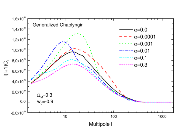
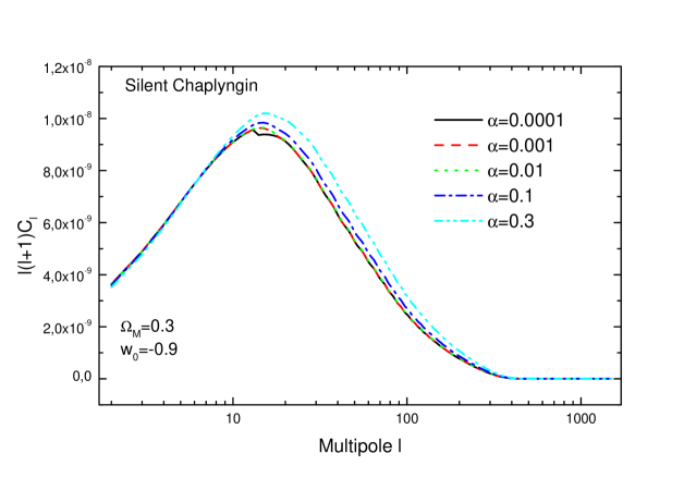
Figure 1: Predictions for the $ISW-LSS$ power spectrum in the case of the generalized (top panel) and silent (bottom panel) Chaplygin. We fix $\Omega_{m}=0.3$ and $w=-0.9$. The LSS survey is centered at $z_{*}=0.3\pm 0.1$.

III Constraints from data

We perform a likelihood analysis using the collection of data presented in Gaztanaga et al. Gaztanaga:2004sk , which has the advantage of being publicly available and easy to implement. In order to avoid degeneracies between the parameters we consider only two possible viable Chaplygin dark energy models: a generalized Chaplygin model with $\alpha=0$ and the silent quintessence model. For those models we vary two parameters: the energy density $\Omega_{Chap}$ and the equation of state $w$.

The data we consider consist of measurements of the average angular cross-correlation around $\theta=5^{\circ}$ between WMAP temperature anisotropy maps and several LSS surveys. The angular average around $\theta=5^{\circ}$ ensures that the signal is not contaminated by foregrounds such as the SZ or lensing effects which are relevant at smaller angles ($\theta\lesssim 1^{\circ}$). Possible systematic contaminants, such as extinction effects, seem not to affect these data and for a more detailed discussion we refer to Gaztanaga:2004sk . The data span a range of redshift $0.1<z\lesssim 1$ and for each redshift bin the data include an estimate of the galaxy bias with $20\%$ errors. These biases are inferred by comparing the galaxy-galaxy correlation function of each experiments with the expectation of best fit model to WMAP power spectra. There is little sensitivity to the scalar spectral index $n_{s}$, while the dependence on the baryon density $\Omega_{b}$ can be non-negligible. In fact the presence of baryons inhibites the growth of CDM fluctuations between matter-radiation equality and photon-baryon decoupling causing the matter power spectrum to be suppressed on scales $k>k_{eq}$ for increasing values of $\Omega_{b}$ ($k_{eq}$ is the scale which enters the horizon at the equality). Over the range of scales which contribute to the ISW-correlation ($k\sim 0.01$) the sensitivity on $\Omega_{b}$ is still present. In order to limit the number of likelihood parameters we therefore assume a Gaussian prior on the baryon density $\Omega_{b}=0.04$ and we take the Hubble parameter as $h=0.7$. We also assume a scale invariant primordial spectrum $n_{s}=1$ and fix the optical depth to reionization to WMAP best fit value $\tau=0.17$ (again the ISW is not particularly affected by a change in those parameters). We marginalize over the normalization amplitude $A_{s}$, although we found no difference assuming the WMAP value. In fact changing $A_{s}$ shifts the overall amplitude of the angular cross-correlation of the same amount over different redshifts but it does not change the redshift dependence of the signal. Since the experimental data are corrected for the bias by comparing the measured galaxy-galaxy correlation function in each redshift bin to the WMAP best fit model, we rescale these biases to each of the dark energy model in our database as described in Gaztanaga:2004sk and cora .

We compute for each theoretical model the angular cross-correlation as described in the previous section using the selection function

$$\phi^{i}(z)\sim z^{2}\exp{[-(z/\bar{z}_{i})^{1.5}]},$$ (18)

where $\bar{z}_{i}$ is the median redshift of the $i$-th survey. Then following Gaztanaga:2004sk , we compute the average cross-correlation in the $i$-th bin, $\bar{C}_{i}^{X}$, around $\theta\sim 5^{\circ}$.

The data points are an average over angles and are infered from surveys whose selection functions may overlap in redshift space, hence they are not independent measurements and indeed are affected by a certain degree of correlation. Since we have no access to the raw data we have no way of accounting for the first type of correlation, while using Eq. (18) we can estimate the correlation between different redshift bins. We compute the correlation matrix $\rho=\{\rho_{ij}\}$, where $\rho_{ij}$ is the fraction of overlapping volume between the $i$-th and $j$-th surveys (i.e. the diagonal components are $\rho_{ii}=1$). To be more conservative we have assumed that the different surveys cover the same fraction of sky, in general this is not the case and the fraction of overlaping volume can be smaller. We found that only two data points are highly correlated, since their selection functions overlap for about $70\%$ in redshift space, while the correlation among the remaining data points are less than $20\%$.

We compute a likelihood function $\cal L$ defined as

$$-2\log{\cal L}=\chi^{2}=\sum_{ij}(\bar{C}_{i}^{X}-{\hat{C}}_{i}^{X})M_{ij}^{-1}(\bar{C}_{j}^{X}-{\hat{C}}_{j}^{X}),$$ (19)

where ${\hat{C}}^{X}_{i}$ are the data and $M_{ij}^{-1}=\rho_{ij}/(\sigma_{i}\sigma_{j})$ is our estimate of the inverse of the covariance matrix, which takes in to account the experimental errors and possible correlation amongst the data, with $\sigma_{i}$ the measured uncertainty in the $i$-th bin.

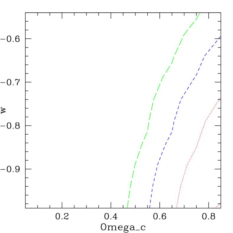
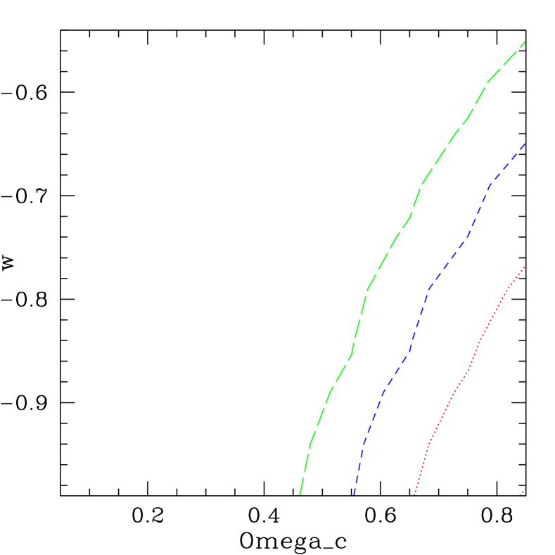
Figure 2: Likelihood contour plots in the $\Omega_{c}$-$w$ plane for a generalized Chaplygin gas with $\alpha=0$ (Top Panel) and for the silent Chaplygin case (Bottom Panel). The contours are $68\%$ (dotted), $95\%$ (short-dashed), $99\%$ (long-dashed) c.l..

The results of our analysis are plotted in Fig. 2 As we can see, in the case of the generalized Chaplygin with $\alpha=0$ the current data constrain $\Omega_{c}>0.55$ and $w<-0.6$ at $95\%$ c.l.. Considering the silent Chaplygin model we obtain similar results with $\Omega_{c}>0.55$ and $w<-0.65$ again at $95\%$ c.l..

IV Conclusions

In this paper we have investigated the possibility of constraining Chaplygin models with the current Integrated Sachs Wolfe effect data. In the case of a flat universe we found that cosmological viable generalized Chaplygin gas models must have an energy density such that $\Omega_{c}>0.55$ and an equation of state $w<-0.6$ at $95\%$ c.l.. We also investigate the recently proposed Silent Chaplygin models, constraining $\Omega_{c}>0.55$ and $w<-0.65$ at $95\%$ c.l.. These constraints have been obtained with a prior on the value of the baryon density $\Omega_{b}$ in agreement with BBN nucleosynthesis. Better measurements of the CMB-LSS correlation will be possible with the next generation of deep redshift surveys. For an ideal whole sky experiment the ISW signal may be detected at the level of $\sim 10\sigma$. This would translate in a factor $2$/$3$ better determination of the results presented here and will provide independent and complementary constraints on unified dark energy models such as the Chaplygin gas.

V Acknowledgments

We thank Pier Stefano Corasaniti and Rachel Bean for valuable help and discussions.

References

- (1) D. N. Spergel et al. [WMAP Collaboration], Astrophys. J. Suppl. 148 (2003) 175 [arXiv:astro-ph/0302209].
- (2) A. Melchiorri, L. Mersini-Houghton, C. J. Odman and M. Trodden, Phys. Rev. D 68 (2003) 043509 [arXiv:astro-ph/0211522]; R. Bean and A. Melchiorri, Phys. Rev. D 65 (2002) 041302 [arXiv:astro-ph/0110472].
- (3) A. Y. Kamenshchik, U. Moschella and V. Pasquier, Phys. Lett. B 511 (2001) 265 [arXiv:gr-qc/0103004].
- (4) S. Chaplygin, Sci. Mem. Moscow Univ. Math. Phys. 21 (1904) 1.
- (5) M. C. Bento, O. Bertolami and A. A. Sen, Phys. Rev. D 66, 043507 (2002) [arXiv:gr-qc/0202064].
- (6) D. Carturan and F. Finelli, Phys. Rev. D 68, 103501 (2003) [arXiv:astro-ph/0211626].
- (7) E. Gaztañaga, M. Manera and T. Multamaki, arXiv:astro-ph/0407022.
- (8) P. S. Corasaniti, T. Giannantonio and A. Melchiorri, Phys. Rev. D 71 (2005) 123521 [arXiv:astro-ph/0504115].
- (9) R. G. Crittenden and N. Turok, Phys. Rev. Lett. 76 (1996) 575 [arXiv:astro-ph/9510072].
- (10) L. Amendola, F. Finelli, C. Burigana and D. Carturan, JCAP 0307 (2003) 005 [arXiv:astro-ph/0304325].
- (11) C. P. Ma and E. Bertschinger, Astrophys. J. 455 (1995) 7 [arXiv:astro-ph/9506072].
- (12) R. Bean and O. Dore, Phys. Rev. D 69 (2004) 083503 [arXiv:astro-ph/0307100].
- (13) R. Bean and O. Dore, Phys. Rev. D 68 (2003) 023515 [arXiv:astro-ph/0301308].
- (14) U. Seljak and M. Zaldarriaga, Astrophys. J. 469 (1996) 437 [arXiv:astro-ph/9603033].
- (15) R. K. Sachs and A. M. Wolfe, Astrophys. J. 147, 73 (1967).
- (16) J. Garriga, L. Pogosian and T. Vachaspati, Phys. Rev. D 69, 063511 (2004) [arXiv:astro-ph/0311412].
- (17) L. Amendola, I. Waga and F. Finelli, JCAP 0511 (2005) 009 [arXiv:astro-ph/0509099].