Cosmology in three dimensions: steps towards the general solution

Abstract

We use covariant and first-order formalism techniques to study the properties of general relativistic cosmology in three dimensions. The covariant approach provides an irreducible decomposition of the relativistic equations, which allows for a mathematically compact and physically transparent description of the 3-dimensional spacetimes. Using this information we review the features of homogeneous and isotropic 3-d cosmologies, provide a number of new solutions and study gauge invariant perturbations around them. The first-order formalism is then used to provide a detailed study of the most general 3-d spacetimes containing perfect-fluid matter. Assuming the material content to be dust with comoving spatial 2-velocities, we find the general solution of the Einstein equations with non-zero (and zero) cosmological constant and generalise known solutions of Kriele and the 3-d counterparts of the Szekeres solutions. In the case of a non-comoving dust fluid we find the general solution in the case of one non-zero fluid velocity component. We consider the asymptotic behaviour of the families of 3-d cosmologies with rotation and shear and analyse their singular structure. We also provide the general solution for cosmologies with one spacelike Killing vector, find solutions for cosmologies containing scalar fields and identify all the PP-wave 2+1 spacetimes.

1 Introduction

General relativity in three spacetime dimensions is known to possess a number of special simplifying features: there are no gravitational waves, no black holes in the absence of a negative cosmological constant, the Weyl curvature is identically zero, and the weak-field limit of the theory does not correspond to Newtonian gravity in two space dimensions [1]-[9]. The theory is therefore considerably ’smaller’ than general relativity spacetimes with four (or more) dimensions, and the strong-energy condition that creates geodesic focussing does not depend on the density of the material sources. These simplifying features mean that considerable progress can be made in the search for the general cosmological solution of the three-dimensional Einstein equations. In an $(N+1)$-dimensional spacetime the number of independently arbitrary $N$-dimensional functions of the space coordinates that are needed to specify the Cauchy data for the general cosmological problem on a spacelike hypersurface in vacuum is $(N+1)(N-2)$; in the presence of a general (non-comoving) perfect fluid it is $N^{2}-1;$ and for a comoving perfect fluid it is $N^{2}-N-1$ [2]. Thus, in the $N=2$ case, we see that the number reduces to zero for the vacuum solution (reflecting the absence of free gravitational fields in vacuum), reduces to one arbitrary spatial function in the comoving perfect-fluid case ,and to three arbitrary spatial functions for a perfect fluid.

In this paper we will set up the general cosmological problem in three-dimensional spacetimes and find the general solution of the field equations in the case of comoving pressure-free matter, with and without a cosmological constant, $\Lambda$. We go on to find solutions for the case of non-comoving dust and classify the singularities and asymptotic behaviours that arise in both cases with and without a cosmological constant. The relative tractability of the general cosmological problem in 2+1 dimensions allows us to go some way towards finding a general solution of the Einstein equations and we are able to isolate those features which prevent a full solution being found. In particular, we are able to find and classify the solutions for dust containing one of the (two possible) non-zero spatial 2-velocity components.

There have been several past investigations of the structure of 2+1 dimensional general relativity and studies of the properties of particular solutions with high symmetry (see [1]-[8], and [10]-[14]). Important motivations for these studies were provided by the astrophysical interest in the possible observational signatures of cosmic strings and domain walls in the universe [15]-[18]. Higher-order curvature contributions were discussed in [2], together with the special features of the Newtonian-relativistic correspondence in general relativity and related theories, while the study of quantum gravity is reviewed in [19]. Cosmological solutions and singularities were discussed in [2] and [20, 21], while gravitational collapse of spherically symmetric dust clouds have been considered in [22]-[24].

The outline of this paper is as follows. In section 2 we define the 3-d Einstein equations and our notations. Section 3 introduces the 2+1 covariant formalism and the general kinematics of 3-d spacetimes, identifying the special features that arise from the lower dimensions and from the vanishing of the Weyl curvature. These include the key role of the isotropic pressure as the sole contributor to the gravitational mass of the system and the fact that vorticity never increases with time. In section 4 we give a number of new cosmological solutions, review the characteristics of the homogeneous and isotropic models, including those that are singularity-free, and provide the generalisation of the Gödel universe to 3 dimensions. We also consider linear perturbations around the 3-d analogues of the ‘dust’-dominated FRW models and find them to be (neutrally) stable. In section 5 we employ Witten’s first-order formalism [25] to formulate the equations governing the most general 3-d cosmological spacetime metric containing perfect-fluid matter. Then, in section 6 we specialise the matter source to pressure-free dust with non-zero $\Lambda$ and comoving 2-velocities and find the general solution of the field equations. These fall into three classes, one of which generalises the solution of Kriele [22] to $\Lambda\neq 0$, while another is the generalisation of the Szekeres metric with nonzero $\Lambda$ to 2+1 dimensions [26, 27]. Section 7 considers the most general dust cosmologies with non-comoving velocities and finds various new classes of solutions. We study the asymptotic behaviour of these solutions and analyse in detail the structure of their spacelike and timelike singularities. Also, by means of a number of examples, we illustrate the wide range of possible behaviours in the presence of vorticity and shear. The same section also introduces a transformation that generates exact solutions with nonzero cosmological constant from those with vanishing $\Lambda$. Finally, in section 8 we look at the case of a pure scalar field, provide the general solution of Einstein’s equations with one spacelike Killing vector, and identify all the 2+1 PP-wave spacetimes. Our results are summarised and discussed in section 9.

2 Einstein’s equations

It has long been known that general relativity, as a theory of a Riemannian spacetime, can be based on a small number of generally accepted postulates which are independent of the spacetime dimensions [28]-[30]. Assuming non-zero cosmological constant, these postulates demand that the field equations take the form

$$R_{ab}-{\textstyle{\frac{1}{2}}}Rg_{ab}+\Lambda g_{ab}=\kappa T_{ab}\,,$$ (1)

where $R_{ab}$ is the Ricci tensor, with $R=R_{a}{}^{a}$, $T_{ab}$ is the energy-momentum tensor of the matter generating the metric field $g_{ab}$, $\Lambda$ is the cosmological constant and $\kappa$ is a dimensional coupling constant. When dealing with 3-dimensional spacetimes $g_{ab}g^{ab}=\delta_{a}{}^{a}=3$. In this geometrical environment $R=-2\kappa T+6\Lambda$, with $T=T_{a}{}^{a}$, and Einstein’s equations become (e.g. see [1, 2])

$$R_{ab}=\kappa(T_{ab}-Tg_{ab})+2\Lambda g_{ab}\,.$$ (2)

The spacetime geometry is determined by the Riemann curvature tensor $R_{abcd}$. In three dimensions the latter has six independent components, exactly as many as the associated Ricci tensor. This means that the spacetime geometry can be expressed solely in terms of the Ricci curvature, namely that [31, 32]

$$R_{abcd}=g_{ac}R_{bd}+g_{bd}R_{ac}-g_{bc}R_{ad}-g_{ad}R_{bc}-{\textstyle{\frac{1}{2}}}R(g_{ac}g_{bd}-g_{ad}g_{bc})\,.$$ (3)

As a result, the 3-dimensional Weyl tensor vanishes identically and the gravitational field has no dynamical degrees of freedom. The spacetime curvature is completely determined by the local matter distribution and the theory is Machian.

3 Covariant decomposition

3.1 Observers

In analogy to the standard 3+1 covariant approach to general relativity introduced by Ehlers [33] and elaborated by Ellis (e.g. see [34] for a recent review), we introduce a family of timelike (fundamental) observers with worldlines tangent to the 3-velocity field $u_{a}$. The latter determines the time direction and is normalised so that $u_{a}u^{a}=-1$. The 2-dimensional space is defined by projecting orthogonal to $u_{a}$ by means of the projection tensor

$$h_{ab}=g_{ab}+u_{a}u_{b}\,,$$ (4)

where $h_{ab}=h_{(ab)}$, $h_{ab}u^{b}=0$, $h_{ab}h^{b}{}_{c}=h_{ac}$ and $h_{a}{}^{a}=2$. Using $h_{ab}$ one also defines the covariant derivative operator of the 2-d space as ${\rm D}_{a}=h_{a}{}^{b}\nabla_{b}$.

The irreducible kinematical variables, which describe the motion of the above defined observers in a invariant way, are obtained by decomposing the covariant derivative of the 3-velocity. This splitting gives

$$\nabla_{b}u_{a}=\sigma_{ab}+\omega_{ab}+{\textstyle{\frac{1}{2}}}\Theta h_{ab}-\dot{u}_{a}u_{b}\,,$$ (5)

where $\sigma_{ab}={\rm D}_{\langle b}u_{a\rangle}$ is the shear, $\omega_{ab}={\rm D}_{[b}u_{a]}$ is the vorticity, $\Theta={\rm D}^{a}u_{a}=\nabla^{a}u_{a}$ is the area expansion (or contraction) scalar and $\dot{u}_{a}=u^{b}\nabla_{b}u_{a}$ the 3-acceleration. Therefore, $\sigma_{ab}u^{b}=0=\omega_{ab}u^{b}=\dot{u}_{a}u^{a}$ by construction.

The tensor ${\rm D}_{b}u_{a}\equiv h_{b}{}^{d}h_{a}{}^{c}\nabla_{d}u_{c}=\sigma_{ab}+\omega_{ab}+(\Theta/2)h_{ab}$ describes changes in the relative position of the worldlines of two neighbouring observers. When the latter follow the motion of a fluid, the effect of $\Theta$ is to change the area of a given fluid element, without causing rotation or shape distortion. This scalar also defines the average scale factor, $a,$ by

$$\frac{\dot{a}}{a}={\textstyle{\frac{1}{2}}}\Theta\,.$$ (6)

The shear monitors distortions in the element’s shape that leave the area unaffected, while $\omega_{ab}$ describes changes in its orientation under constant area and shape. The symmetric and trace-free nature of $\sigma_{ab}$ ensures that it has only two independent components, while the antisymmetry of $\omega_{ab}$ guarantees that the vorticity tensor is determined by a single component. In other words, the shear and the vorticity correspond to a vector and a scalar respectively. The latter reflects the fact that the rotational axis has been reduced to a point. Defining $\epsilon_{ab}=\epsilon_{[ab]}$ as the 2-dimensional permutation tensor, with $\epsilon_{ab}u^{b}=0$, the vorticity scalar is

$$\omega={\textstyle{\frac{1}{2}}}\epsilon_{ab}\omega^{ab}\,,$$ (7)

with $\omega_{ab}=\omega\epsilon_{ab}$. Note that $\epsilon_{ab}=\eta_{abc}u^{c}$ by definition, where $\eta_{abc}$ is the 3-d totally antisymmetric alternating tensor. The latter satisfies the condition $\eta_{abc}\eta^{dqs}=3!\delta_{[a}{}^{d}\delta_{b}{}^{q}\delta_{c]}{}^{s}$, which ensures that $\epsilon_{ab}\epsilon^{cd}=2h_{[a}{}^{c}h_{b]}{}^{d}$.

3.2 Matter fields

Suppose that the matter that sources the 3-dimensional metric field is a perfect fluid. Then, relative to an observer moving with 3-velocity $u_{a}$, the energy-momentum tensor of the material component takes the form

$$T_{ab}=\rho u_{a}u_{b}+ph_{ab}\,,$$ (8)

where $\rho$ is the energy density, $p$ is pressure and its trace is $T=2p-\rho$. Substituting the above into the Einstein field equations (2) the latter read

$$R_{ab}=2(\kappa p-\Lambda)u_{a}u_{b}+[\kappa(\mu-p)+2\Lambda]h_{ab}\,,$$ (9)

with trace $R=2[\kappa(\mu-2p)+3\Lambda]$. The above also provides the following auxiliary relations

$$R_{ab}u^{a}u^{b}=2(\kappa p-\Lambda)\,,\hskip 28.45274pth_{a}{}^{c}h_{b}{}^{d}R_{cd}=[\kappa(\rho-p)+2\Lambda]h_{ab}\hskip 14.22636pt{\rm and}\hskip 14.22636pth_{a}{}^{b}R_{bc}u^{c}=0\,$$ (10)

which will prove useful later.

The twice-contracted Bianchi identities imply that $\nabla^{b}G_{ab}=0$ and consequently the condition $\nabla^{b}T_{ab}=0$. The timelike and spacelike parts of the latter lead to the 3-d fluid conservation laws. These are

$$\dot{\rho}=-\Theta(\rho+p)\,,$$ (11)

for the energy density of the fluid, and

$$(\rho+p)\dot{u}_{a}=-{\rm D}_{a}p$$ (12)

for its momentum density. The above ensure that the conservation laws of a perfect fluid have the same functional form as their 4-dimensional counterparts (compare to Eqs. (37), (38) of [34]).

The nature of the medium is determined by its equation of state. Here we will only consider barotropic fluids with $p=w\rho$, where $w$ represents the barotropic index. When $w=0$ we are dealing with pressure-free dust, while isotropic radiation has $p=\rho/2$ and corresponds to $w=1/2$ [1].

3.3 Spatial curvature

The intrinsic curvature of the 2-dimensional space orthogonal to $u_{a}$ is determined by the associated Riemann tensor. In analogy with its standard 3-d counterpart (see Eq. (77) in [35]), the latter is defined by

$${\cal R}_{abcd}=h_{a}{}^{q}h_{b}{}^{s}h_{c}{}^{f}h_{d}{}^{p}R_{qsfp}-v_{ac}v_{bd}+v_{ad}v_{bc}\,,$$ (13)

where

$$v_{ab}={\rm D}_{b}u_{a}=\sigma_{ab}+\omega_{ab}+{\textstyle{\frac{1}{2}}}\Theta h_{ab}\,,$$ (14)

is the relative position vector. Note that $v_{ab}$ characterises the extrinsic curvature (i.e. the second fundamental form) of the space.

Starting from Eq. (13), assuming perfect-fluid matter and using expressions (3), (9), (10) and (14), the Riemann tensor of the 2-d (spatial) sections reads

$${\cal R}_{abcd} = \left(\kappa\rho-{\textstyle{\frac{1}{4}}}\Theta^{2}+\Lambda\right)(h_{ac}h_{bd}-h_{ad}h_{bc})-(\sigma_{ac}+\omega_{ac})(\sigma_{bd}+\omega_{bd})+(\sigma_{ad}+\omega_{ad})(\sigma_{bc}+\omega_{bc})$$ (15)

$$-{\textstyle{\frac{1}{2}}}\Theta\left[(\sigma_{ac}+\omega_{ac})h_{bd}+h_{ac}(\sigma_{bd}+\omega_{bd})-(\sigma_{ad}+\omega_{ad})h_{bc}-h_{ad}(\sigma_{bc}+\omega_{bc})\right]\,,$$

with ${\cal R}_{abcd}={\cal R}_{[ab][cd]}$. In agreement with standard 3+1 gravity, the isotropic pressure does not contribute to the curvature of the space orthogonal to $u_{a}$. Also, in the absence of anisotropy (i.e. when $\sigma_{ab}$ and $\omega_{ab}$ vanish) the above reduces to

$${\cal R}_{abcd}=\left(\kappa\rho-{\textstyle{\frac{1}{4}}}\Theta^{2}+\Lambda\right)(h_{ac}h_{bd}-h_{ad}h_{bc})\,.$$ (16)

Defining ${\cal R}_{ab}={\cal R}^{c}{}_{acb}$ as our local 2-D Ricci tensor, we may contract expression (15) to obtain the following 3-dimensional analogue of the Gauss-Codacci formula (see Eq. (54) in [34])

$${\cal R}_{ab}=\left(\kappa\rho-{\textstyle{\frac{1}{4}}}\Theta^{2}+\sigma^{2}-\omega^{2}+\Lambda\right)h_{ab}\,,$$ (17)

which here holds for perfect-fluid matter. In deriving the above we used the results $\omega_{c[a}\sigma^{c}{}_{b]}=0$ and $\sigma_{c\langle a}\sigma^{c}{}_{b\rangle}=0=\omega_{c\langle a}\omega^{c}{}_{b\rangle}$. The former holds because $\omega_{12}(\sigma^{1}{}_{1}+\sigma^{2}{}_{2})=0$ (i.e. the single independent component vanishes due to the trace-free nature of the shear). Similarly, the two independent components of $\sigma_{c\langle a}\sigma^{c}{}_{b\rangle}$ are also identically zero. Last, the result $\omega_{c\langle a}\omega^{c}{}_{b\rangle}=0$ is guaranteed by the relation $\omega_{ab}=\omega\epsilon_{ab}$ and the properties of $\epsilon_{ab}$ (see section 3.1). The absence of a skew and also of a symmetric and trace-free part from Eq. (17) agrees with symmetries of the Riemann tensor in 2-d spaces (e.g. see [1]).

Finally, the trace of (17) leads to the curvature scalar of the spatial sections, which may also be seen as the generalised Friedmann equation for three-dimensional spacetimes (compare to Eq. (55) of [34])

$${\cal R}\equiv{\cal R}^{a}{}_{a}=2\left(\kappa\rho-{\textstyle{\frac{1}{4}}}\Theta^{2}+\sigma^{2}-\omega^{2}+\Lambda\right)\,.$$ (18)

3.4 Kinematics

The functional form of the Ricci identity is independent of dimension. Thus, when applied to the 3-velocity vector $u_{a},$ the Ricci identity reads

$$\nabla_{a}\nabla_{b}u_{c}-\nabla_{b}\nabla_{a}u_{c}=R_{abcd}u^{d}\,,$$ (19)

where $R_{abcd}$ is the Riemann tensor of the 3-d spacetime (see expression (3)). Contracting the above along $u_{b}$, employing Eqs. (3), (10), and then taking the trace of the resulting expression we obtain the 3-d analogue of Raychaudhuri’s equation

$$\dot{\Theta}=-{\textstyle{\frac{1}{2}}}\Theta^{2}-2\kappa p-2(\sigma^{2}-\omega^{2})+{\rm D}^{a}\dot{u}_{a}+\dot{u}^{a}\dot{u}_{a}+2\Lambda\,,$$ (20)

with $2\sigma^{2}\equiv\sigma_{ab}\sigma^{ab}$ and $2\omega^{2}\equiv\omega_{ab}\omega^{ab}$. The above is the key equation of gravitational attraction, as it monitors the average separation between neighbouring particle worldlines. The most important difference between (20) and its 4-d counterpart (see Eq. (29) in [34]) is that here only the fluid pressure contributes to the gravitational mass of the medium: the density $\rho$ does not contribute. This unusual feature consists a major departure from standard gravity. One consequence is the existence of homogeneous and isotropic static 3-dimensional models with dust and zero cosmological constant (see solution (29) below).

The symmetric and trace-free part of the contracted Ricci identity, together with the auxiliary relations (10) leads to the propagation formula for the shear in three dimensions:

$$h_{a}{}^{c}h_{b}{}^{d}\dot{\sigma}_{cd}=-\Theta\sigma_{ab}+{\rm D}_{\langle b}\dot{u}_{a\rangle}+\dot{u}_{\langle a}\dot{u}_{b\rangle}\,.$$ (21)

Relative to the 4-dimensional case (see Eq. (30) in [34]), we notice the absence of the electric Weyl component from the right-hand side of this formula. This reflects the vanishing of the free gravitational field in 3-d gravity. Contracting this expression with $\sigma_{ab}$ we obtain the propagation formula for the shear magnitude

$$\left(\sigma^{2}\right)^{\cdot}=-2\Theta\sigma^{2}+\sigma^{ab}{\rm D}_{\langle b}\dot{u}_{a\rangle}+\dot{u}_{\langle a}\dot{u}_{b\rangle}\sigma^{ab}\,,$$ (22)

where $2\sigma^{2}=\sigma_{ab}\sigma^{ab}$ by definition. In the absence of fluid accelerations the 2nd and 3rd terms on the right-hand side vanish and the equation integrates to give $\sigma^{2}\propto a^{-4}$.

Similarly, the contracted antisymmetric component of (19) gives the 3-d counterpart of the vorticity propagation equation. The latter reads

$$h_{a}{}^{c}h_{b}{}^{d}\dot{\omega}_{cd}=-\Theta\omega_{ab}+{\rm D}_{[b}\dot{u}_{a]}\,.$$ (23)

Comparing to Eq. (31) of [34] we note the absence of the $\omega_{c[a}\sigma^{c}{}_{b]}$ term. This is so because $\omega_{c[a}\sigma^{c}{}_{b]}=0$ in 3-d (see also above). Also, contracted with $\omega_{ab}$, and recalling that $2\omega^{2}\equiv\omega_{ab}\omega^{ab}$ Eq. (23) gives the scalar vorticity propagation formula:

$$\left(\omega^{2}\right)^{\cdot}=-2\Theta\omega^{2}+\omega^{ab}{\rm D}_{[b}\dot{u}_{a]}\,.$$ (24)

Again, in the absence of accelerations when the pressure vanishes this equation integrates to give $\omega^{2}\propto a^{-4}$ as expected by the conservation of angular momentum. For a barotropic perfect fluid with $p=p(\rho)$ and a constant barotropic index $w=p/\rho$, Eqs. (11), (12) combine with the commutation law ${\rm D}_{[a}{\rm D}_{b]}f=-\dot{f}\omega_{ab}$ to recast the vorticity propagation formula as

$$h_{a}{}^{c}h_{b}{}^{d}\dot{\omega}_{cd}=-(1-c_{{\rm s}}^{2})\Theta\omega_{ab}\,,$$ (25)

where $c_{{\rm s}}^{2}={\rm d}p/{\rm d}\rho=w$ is the square of the adiabatic sound speed. Therefore, the expansion decreases the vorticity of a 2-dimensional space unless the barotropic fluid has a stiff equation of state (i.e. when $c_{{\rm s}}^{2}=1=w$) and for general perfect fluids we have $\omega^{2}\propto a^{-2(1-w)}$. Recall that, in standard general relativity, vorticity increases when $w>2/3$ [36].

The simultaneous effects of shear and vorticity on a cosmology with negligible accelerations can be evaluated from these simple relations. For all equations of state we have $\sigma^{2}\propto a^{-4}$ but the centrifugal energy depends on the equation of state since $\omega^{2}\propto a^{-4(1-w)}$. Hence, the ratio of the distortion energy density to the centrifugal energy density is

$$\frac{\sigma^{2}}{\omega^{2}}\propto a^{-2w}$$

and the shear always dominates as $a\rightarrow 0$ when $p>0$ but the vorticity always dominates as $a\rightarrow\infty$. The presence of fluid acceleration can modify this behaviour; an example with $p=0$ will be given below.

4 Cosmology in 2+1 dimensional spacetimes

4.1 Homogeneous and isotropic spacetimes

Spatial homogeneity and isotropy means that we can always choose a coordinate system such as the line element of the 3-dimensional spacetime takes the Friedmann-Robertson-Walker (FRW) form

$${\rm d}s^{2}=-{\rm d}t^{2}+a^{2}h_{\alpha\beta}{\rm d}x^{\alpha}{\rm d}x^{\beta}\,,$$ (26)

where the scale factor $a=a(t)$ completely determines the time evolution of the model. The form also represents the metric of the 3-dimensional analogue of the familiar FRW cosmologies. The kinematics of (26) is monitored via one propagation and one constraint equation (see expressions (20) and (18)). Assuming a barotropic fluid with with constant barotropic index, setting $\Lambda=0$ and recalling that $\Theta=2\dot{a}/a$, these formulae recast into

$$\frac{\ddot{a}}{a}=-2\kappa w\rho\hskip 42.67912pt{\rm and}\hskip 42.67912pt\left(\frac{\dot{a}}{a}\right)^{2}=\kappa\rho-\frac{k}{a^{2}}\,,$$ (27)

respectively ($k=0,\,\pm 1$ is the curvature index of the spatial sections). The matter component obeys the conservation law (11), which accepts the solution

$$\rho=\rho_{0}\left(\frac{a_{0}}{a}\right)^{2(1+w)}\,,$$ (28)

with $a_{0}$ constant.

For dust, $w=0,$ and one immediately finds (see Eq. (27a)) that $a\propto t$ for all signs of $k$. More specifically, expression (28) gives $\rho\propto a^{-2}$, which substituted into Eq. (27b) leads to

$$a=\left(\kappa\rho_{0}a_{0}^{2}-k\right)^{1/2}t+a_{0}\,,$$ (29)

where the product $\rho_{0}a_{0}^{2}$ is proportional to the total mass of the model. Therefore, the scale factor of a dust-dominated, 3-dimensional, FRW universe evolves linearly with time, irrespective of its spatial curvature and no collapse to a final singularity occurs. Note that when $\kappa\rho_{0}a_{0}^{2}=k$ we obtain a static solution with $a=a_{0}$ [1]. Unlike its 4-d counterparts, this static universe has zero cosmological constant (see also section 5 above).

When the matter content is in the form of black-body radiation, the barotropic index is $w=1/2$. Then, expression (28) gives $\rho\propto a^{-3}$ and the system (27) has the solution

$$a=\int\sqrt{\frac{\kappa\rho_{0}a_{0}^{3}-ka}{a}}\,{\rm d}t+a_{0}\,.$$ (30)

For $k=0$ the above reduces to $a\propto t^{2/3}$, which coincides with the scale-factor evolution in standard 3+1 dust-dominated FRW universes.

One can study perturbations around the above given homogeneous and isotropic solutions by introducing the covariantly defined variables ${\cal D}_{a}=(a/\rho){\rm D}_{a}\rho$ and ${\cal Z}_{a}=a{\rm D}_{a}\Theta$. The former describes variations in the matter density and the latter in the area expansion as measured by a pair of neighbouring observers [37]. Also, both variables vanish in the spatially homogeneous background and therefore satisfy the gauge-invariance criterion. In the case of a pressureless fluid (i.e. for $w=0=c_{{\rm s}}^{2}$) the linear evolution of inhomogeneities is monitored by

$$\dot{{\cal D}}=-{\cal Z}\hskip 28.45274pt{\rm and}\hskip 28.45274pt\dot{{\cal Z}}=-\Theta{\cal Z}\,,$$ (31)

on all scales. Then, using solution (29) and setting ${\cal D}_{0}=(\alpha t_{0}+a_{0}){\cal Z}_{0}/\alpha$ initially, we find that the density gradient decays as

$${\cal D}={\cal D}_{0}\left(\frac{\alpha t_{0}+a_{0}}{\alpha t+a_{0}}\right)\,,$$ (32)

with $\alpha=\sqrt{\kappa\rho_{0}a_{0}^{2}-k}$ and $k=0,\pm 1$ (see (29)). For general initial conditions, on the other hand, it is straightforward to show that ${\cal D}\rightarrow{\cal D}_{0}-(\alpha t_{0}+a_{0}){\cal Z}_{0}/\alpha$ at late times. Recalling that for zero pressure shear and vorticity perturbations decay in time (see Eqs. (21) and (23)), we conclude that in the absence of pressure the 3-d analogues of the FRW cosmologies are either stable or neutrally stable. This behaviour is very different from that of conventional FRW models, all of which are unstable to density perturbations, and reflects the fact that in three dimensions the gravitational mass of a pressure-free medium vanishes (see Eq. (20)) and spherical regions of all curvatures asymptote to $a\rightarrow t$ as $t\rightarrow\infty$. The immediate consequence is the absence of linear Jeans-type instabilities in these models.

4.2 Homogeneous and anisotropic spacetimes

The simplest 3-d line element describing a homogeneous and anisotropic spacetime has the following Bianchi I-type form

$${\rm d}s^{2}=-{\rm d}t^{2}+A^{2}{\rm d}x^{2}+B^{2}{\rm d}y^{2}\,,$$ (33)

where $A=A(t)$ and $B=B(t)$ are the two individual scale factors. When $\Lambda=0$, the spatial flatness of the above metric means that the 3-d analogue of the Bianchi I universe is covariantly described by the following set of propagation equations

$$\dot{\rho}=-(1+w)\Theta\rho\,,\hskip 42.67912pt\dot{\Theta}=-{\textstyle{\frac{1}{2}}}\Theta^{2}-2\kappa w\rho-2\sigma^{2}\,,\hskip 42.67912pt\dot{\sigma}=-\Theta\sigma\,,\text{ \ \ \ \ \ \ \ \ }\omega\equiv 0$$ (34)

supplemented by the constraint

$${\textstyle{\frac{1}{4}}}\Theta^{2}=\kappa\rho+\sigma^{2}\,.$$ (35)

The above are obtained from Eqs. (11), (20), (22) and (18), respectively, after dropping their inhomogeneous terms and assuming spatial flatness together with zero vorticity. Setting $\Theta=2\dot{a}/a$, where $a$ represents the geometric-mean scale factor, expressions (34a) and (34c) lead to the evolution laws

$$\rho=\rho_{0}\left(\frac{a_{0}}{a}\right)^{2(1+w)}\hskip 28.45274pt{\rm and}\hskip 28.45274pt\sigma=\sigma_{0}\left(\frac{a_{0}}{a}\right)^{2}\,,$$ (36)

for the matter energy density and the shear respectively. Substituting these results to Eq. (35) and assuming a spacetime filled with pressure-free dust we arrive at

$$a=a_{0}\sqrt{\kappa\rho_{0}t^{2}+2\sigma_{0}t}\,.$$ (37)

As expected, for $\sigma_{0}=0$ the above result reduces to its isotropic counterpart (see Eq. (29)). The same also happens at late times, when the shear contribution to solution (37) becomes negligible.

Note that one can use the evolution law of the average scale factor to obtain those of the individual ones. Assuming dust, recalling that

$$\frac{\dot{A}}{A}+\frac{\dot{B}}{B}=\Theta\hskip 42.67912pt{\rm and}\hskip 42.67912pt\frac{\dot{A}}{A}-\frac{\dot{B}}{B}=2\sigma\,,$$ (38)

and using results (36c) and (37) we arrive at

$$A=A_{0}\left(\frac{t}{t_{0}}\right)\hskip 42.67912pt{\rm and}\hskip 42.67912ptB=B_{0}\left(\frac{\kappa\rho_{0}t+2\sigma_{0}}{\kappa\rho_{0}t_{0}+2\sigma_{0}}\right)\,.$$ (39)

In the vacuum case ($\rho_{0}\equiv 0$) the metric is just a coordinate transformation of flat spacetime rather than an anisotropic cosmology.

4.3 Rotating spacetimes

Consider a rotating three-dimensional spacetime with flat 2-d sections filled with pressureless matter. Setting $\Lambda=0$ and assuming spatial homogeneity, the time evolution of the model (at least locally) is monitored by the following system of four propagation equations

$$\dot{\rho}=-\Theta\rho\,,\hskip 28.45274pt\dot{\Theta}=-{\textstyle{\frac{1}{2}}}\Theta^{2}-2\sigma^{2}+2\omega^{2}\,,\hskip 28.45274pt\dot{\sigma}=-\Theta\sigma\hskip 28.45274pt{\rm and}\hskip 28.45274pt\dot{\omega}=-\Theta\omega\,,$$ (40)

constrained by

$${\textstyle{\frac{1}{4}}}\Theta^{2}=\kappa\rho+\sigma^{2}-\omega^{2}\,.$$ (41)

Proceeding as before, we may use the area expansion scalar ($\Theta$) to define an average scale factor ($a$) so that $\Theta=2\dot{a}/a$. Then, expressions (40a), (40b) and (40c) translate into

$$\rho=\rho_{0}\left(\frac{a_{0}}{a}\right)^{2}\,,\hskip 28.45274pt\sigma=\sigma_{0}\left(\frac{a_{0}}{a}\right)^{2}\hskip 28.45274pt{\rm and}\hskip 28.45274pt\omega=\omega_{0}\left(\frac{a_{0}}{a}\right)^{2}$$ (42)

respectively. Substituted into constraint (41) the above results give

$$a=a_{0}\sqrt{\kappa\rho_{0}t^{2}+2t\sqrt{\sigma_{0}^{2}-\omega_{0}^{2}}}\,.$$ (43)

Accordingly, despite the presence of nonzero shear and vorticity, the average scale factor evolves as its homogeneous and isotropic counterpart if $\sigma_{0}=\omega_{0}$. The situation in 3-d is unusual in that the shear and vorticity scale as the same powers of the scale factor and are both equally important at all times. In the case of dust, the matter density also scales as $a^{-2}$ (see (42)).

One can also obtain a 3-d Gödel-type universe. The Gödel spacetime is a homogeneous spacetime and a rotating solution of Einstein’s equations which permits closed timelike curves [38, 39]. Covariantly, Gödel’s world is described by [40, 41]

$$\Theta=0=\dot{u}_{a}=\sigma_{ab}\hskip 28.45274pt{\rm and}\hskip 28.45274pt\omega_{ab}\neq 0\,.$$ (44)

Thus, with the exception of the vorticity, all the kinematical variables vanish identically. Note that the overall homogeneity of the Gödel spacetime guarantees that the vorticity is a covariantly constant quantity and that all the propagation equations reduce to constraints. Applying (44) to three dimensions we arrive at the system

$$\dot{\rho}=0\,,\hskip 28.45274pt\dot{\omega}=0\,,\hskip 28.45274pt\kappa p-\omega^{2}-\Lambda=0\hskip 28.45274pt{\rm and}\hskip 28.45274pt{\cal R}=2(\kappa\rho-\omega^{2}+\Lambda)\,.$$ (45)

which describes a 3-d Gödel-type universe. Note that for pressure-free matter the cosmological constant is necessarily negative (i.e. $\Lambda=-\omega^{2}$ - see Eq. (45c)). Also, unlike its standard 3+1 counterpart, the 3-dimensional Gödel-type spacetime can have non-vanishing spatial Ricci curvature. This is guaranteed by (45d). The empty Gödel-type model with ${\cal R}=-4\omega^{2}<0$ is equivalent to anti-de Sitter (AdS) space. Rooman and Spindel, [42], considered a one-parameter subset of these non-flat Gödel-type solutions and showed that they can be seen as arising from a directional squashing of the light cones of AdS, which breaks the ${\mathfrak{s}o}(2,2)$ isometry of the AdS Killing vectors into ${\mathfrak{s}o}(2,1)\times{\mathfrak{s}o}(2)$. It was shown in [42] that all the non-empty Gödel-type solutions considered contained closed-timelike curves but they vanish in the AdS limit.

4.4 Singularities

The 3-d analogues of the standard singularity theorems are relatively straightforward to deduce. The study of the Riemann and the Ricci curvature shows that there are no Weyl curvature singularities and the analogue of the strong-energy condition (i.e. $R_{ab}u^{a}u^{b}\geq 0$) reduces to the inequality $p\geq 0$ for a perfect fluid and to the positivity of the sum of the principal pressures if they are anisotropic. Also, the form of the Raychaudhuri equation (see (20)) guarantees that for geodesically moving observers

$$\dot{\Theta}+{\textstyle{\frac{1}{2}}}\Theta^{2}=-2\kappa p-2(\sigma^{2}-\omega^{2})+2\Lambda\,.$$ (46)

Therefore, for vanishing cosmological constant and in the absence of rotation, an initially converging family of timelike worldlines will focus (i.e. $\Theta\rightarrow-\infty$). For non-zero vorticity, however, this may not be necessarily the case. For example, applied to a spatially homogeneous and rotating spacetime filled with an isotropic radiation fluid, the above gives

$$\dot{\Theta}+{\textstyle{\frac{1}{2}}}\Theta^{2}=-\kappa\rho_{0}\left(\frac{a_{0}}{a}\right)^{3}-2(\sigma_{0}^{2}-\omega_{0}^{2})\left(\frac{a_{0}}{a}\right)^{4}\,.$$ (47)

Therefore, as $a\rightarrow 0$, the kinematical term dominates the matter term in the right-hand side of the Raychaudhuri equation. In this case, whether caustics will form or not depends entirely on the balance between shear and rotation. When $\omega_{0}>\sigma_{0}$, in particular, vorticity can stop an initially converging family of worldlines from focusing.

There are also simple exact solutions that describe ‘bouncing’ 3-d cosmologies with $p<0$. Consider, for example, a perfect fluid with $p=-\rho/2$. Then, assuming spatial homogeneity and isotropy, Eq. (11) gives $\rho\propto a^{-1}$ and the Friedmann equation reduces to

$$\left(\frac{\dot{a}}{a}\right)^{2}=\frac{M}{a}-\frac{k}{a^{2}}\,,$$ (48)

where $M>0$ is constant and $k$ is the spatial curvature index. The bouncing solution is

$$a(t)=a_{{\rm min}}+{\textstyle{\frac{1}{4}}}M\left(t-t_{{\rm min}}\right)^{2}\,,$$ (49)

with $a_{{\rm min}}=k/M$. Accordingly, a non-singular minimum requires positive curvature. Setting $k=+1$ and $t_{{\rm min}}=0$ the required scale-factor evolution is represented by the parabola

$$a(t)=M^{-1}+{\textstyle{\frac{1}{4}}}Mt^{2}\,.$$ (50)

5 First-Order Formalism

In 2+1 dimensions it has been shown by Witten [25] that the Palatini action for general relativity is equivalent to:

$$S_{g}=\int\tilde{\eta}^{abc}e_{a}^{I}\,{}^{3}F_{bcI}$$ (51)

where $\tilde{\eta}^{abc}$ is the metric-independent alternating symbol in $2+1$ dimensions. Recall, our signature is $(-++)$ and we choose $\tilde{\eta}^{012}=-1\Rightarrow\tilde{\eta}_{012}=+1$; $e_{a}^{I}$ is a dreibein, and in some sense should be viewed as the square root of the metric

$$g_{ab}=e_{a}^{I}e_{b}^{J}\eta_{IJ},$$

where $\eta_{IJ}=diag(-1+1+1)$. We set

$${}^{3}F_{abI}=2\partial_{[a}{}^{3}A_{b]}^{I}+\epsilon_{IJK}{}^{3}A_{a}^{J}\,{}^{3}A_{b}^{K},$$

where ${}^{3}A_{a}^{I}$ is an $SO(2,1)$ connection, and $\epsilon_{IJK}$ is the standard alternating symbol. Here $a,b=0,1,2$ are spacetime indices, whilst $I,J,K=\hat{0},\hat{1},\hat{2}$ are internal $SO(2,1)$ indices. We raise and lower internal indices with $\eta_{IJ}$ and $\eta^{IJ}$, so $\epsilon^{IJK}=-\epsilon_{IJK}$, and we choose $\epsilon_{\hat{0}\hat{1}\hat{2}}=+1$. The action (51) reduces to the standard second-order gravitational action when ${}^{3}A_{a}^{I}$ is compatible with $e_{a}^{I}$ i.e.

$${\cal D}_{[a}e_{b]I}:=\partial_{[a}e_{b]I}+\epsilon_{IJK}\,{}^{3}A_{[a}^{J}e_{b]}^{K}=0.$$ (52)

We could also find this equation by varying the above action w.r.t. ${}^{3}A_{a}^{I}$. There is plenty of gauge freedom in this model, so we firstly simplify matters by choosing to write the metric in synchronous gauge as

$${\rm d}s^{2}=g_{ab}{\rm d}x^{a}{\rm d}x^{b}=-{\rm d}t^{2}+h_{\alpha\beta}{\rm d}x^{\alpha}{\rm d}x^{\beta},$$ (53)

where $\alpha,\beta=1,2$. In synchronous gauge: $e_{0}^{\hat{0}}=1$, $e_{0}^{i}=0$, $e_{\alpha}^{\hat{0}}=0$, where $i=\hat{1},\hat{2}$ are 2-d internal indices. Throughout this section, we will use $a,b,c,d$ to designate 3-d spacetime indices, and $I,J,K$ for 3-d internal indices. Lower case Greek letters will be used for 2-d spacetime indices, and $i,j,k$ for 2-d internal ones. We define a projection operator onto the surfaces $t=const$ by

$$h_{ab}=g_{ab}+n_{a}n_{b}$$ (54)

where $n_{a}=(1,0,0)$ and $h_{ab}=h_{\alpha\beta}$ is the induced metric on the spacelike surfaces defined by $t=const$. We make some further definitions:

$$E_{\alpha}^{i} = h_{\alpha}^{\beta}e_{\beta}^{i},$$ (55)

$$A_{a}^{i} = h_{\alpha}^{\beta}{}^{3}A_{\beta}^{i},$$ (56)

$$B_{a} = h_{\alpha}^{\beta}{}^{3}A_{\beta\hat{0}},$$ (57)

$$F_{\alpha\beta I} = h_{\alpha}^{\gamma}h_{\beta}^{\delta}{}^{3}F_{\gamma\delta I},$$ (58)

$$(n\cdot A)^{I} = n^{a}{}^{3}A_{a}^{I}.$$ (59)

We can also use the gauge freedom in the definition of ${}^{3}A_{a}^{I}$ to set $(n\cdot A)^{\hat{0}}=0$, and do so. We are still left with the freedom to make $SO(2)$ rotations on the internal indices, $i=1,2$, with the angle of rotation an arbitrary function of the spatial coordinates, ($x,y$).

5.1 Field Equations

In 2+1 spacetime dimensions:

$$R_{abcd} = R_{ac}g_{bd}-R_{ad}g_{bc}+R_{bd}g_{ac}-R_{bc}g_{ad}+\left(\frac{R}{2}\right)\left(g_{ad}g_{bc}-g_{ac}g_{bd}\right),$$ (60)

$$R_{ab} = \kappa(T_{ab}-Tg_{ab}),$$ (61)

$$R = -2\kappa T.$$ (62)

So, therefore:

$$R_{abcd}=\kappa\left[T_{ac}g_{bd}-T_{ad}g_{bc}+T_{bd}g_{ac}-T_{bc}g_{ad}+T\left(g_{ad}g_{bc}-g_{ac}g_{bd}\right)\right],$$

where the curvature ${}^{3}F_{abI}$ is related to the $R_{abcd}$ by

$${}^{3}F_{abI}=R_{abcd}e^{cJ}e^{dK}\epsilon_{IJK}.$$

We define: $T^{IJ}=e^{aI}e^{bJ}T_{ab}$, so the Einstein equations can then be written as:

$${\cal D}_{[a}e_{b]I} = 0,$$ (63)

$${}^{3}F_{abI} = \kappa\left[2e_{[a}^{L}e_{b]}^{K}T_{L}^{J}\epsilon_{IJK}-Te_{a}^{J}e_{b}^{K}\epsilon_{IJK}\right].$$ (64)

Note that these equations remain well-defined even if $det(e)=\sqrt{-g}=0$, so in this form the field equations actually describe a theory that is more general than general relativity. When $e_{a}^{I}$ is invertible, however, these field equations are fully equivalent to 3-d general relativity. We are concerned with the dynamics of perfect-fluid spacetimes and for the purposes of this section will consider only dust models, $p=0$, so $T^{IJ}=\kappa\rho u^{I}u^{J}-\Lambda\eta^{IJ}$, where $u_{K}u^{K}=-1$. We write $u^{k}=U^{k}=U_{k}$ and $u_{\hat{0}}=1+U_{k}U^{k}$, $k=1,2$.

5.2 2+1 decomposition of field equations

We now use $n^{a}$ and $h_{b}^{a}$ to decompose the field equations. From equation (63) we find that $n\cdot A^{i}=0$ and:

$$\dot{E}_{\alpha i}=\epsilon_{ij}A_{\alpha}^{j},$$ (65)

$$\tilde{\eta}^{\alpha\beta}\partial_{\alpha}E_{\beta i}+\epsilon_{ij}B_{\alpha}E_{\beta}^{j}\tilde{\eta}^{\alpha\beta}=0,$$ (66)

$$\tilde{\eta}^{\alpha\beta}\epsilon_{ij}A_{\alpha}^{i}E_{\beta}^{j}=0,$$ (67)

and by projecting equation (64) we arrive at:

$$\dot{B}_{\alpha} = \kappa\rho u_{\hat{0}}U^{i}\epsilon_{ij}E_{\alpha}^{j},$$ (68)

$$\dot{A}_{\beta i} = \kappa\rho\left[U_{k}U_{k}\epsilon_{ij}E_{\beta}^{j}-U_{l}E_{\beta}^{l}\epsilon_{ij}U^{j}\right]-\Lambda\epsilon_{ij}E_{\beta}^{j},$$ (69)

$$\tilde{\eta}^{\alpha\beta}\partial_{\alpha}A_{\beta i}+\epsilon_{ij}B_{\alpha}A_{\beta}^{j}\tilde{\eta}^{\alpha\beta} = -\kappa\rho u_{\hat{0}}U^{j}\epsilon_{jk}E_{\alpha}^{k}E_{\beta i}\tilde{\eta}^{\alpha\beta},$$ (70)

$$\tilde{\eta}^{\alpha\beta}(2\partial_{\alpha}B_{\beta}+\epsilon_{ij}A_{\alpha}^{i}A_{\beta}^{j}) = \kappa\rho\left[2E_{\alpha}^{k}E_{\beta}^{j}\tilde{\eta}^{\alpha\beta}U_{k}U^{i}\epsilon_{ij}+E_{\alpha}^{i}E_{\beta}^{j}\tilde{\eta}^{\alpha\beta}\epsilon_{ij}\right]+\Lambda\epsilon_{ij}E_{\alpha}^{i}E_{\beta}^{j}\tilde{\eta}^{\alpha\beta}.$$ (71)

Equations (65), (68) and (69) provide 10 evolution equations for the ten degrees of freedom contained in the $E_{\alpha}^{i}$, $B_{\alpha}$ and $A_{\alpha}^{i}$. To solve these we must specify these quantities, as well as $\rho$ and the $U^{i}$, on some initial spacelike hypersurface: a total of 13 initial functions. The other equations amount to 6 consistency conditions, which restricts the number of free functions to 7. We may still make 3 coordinate transforms, and 1 internal $SO(2)$ rotation, or gauge transform. This brings us down to $3$ functions that may be freely specified on the initial surface; we take these to be $\rho$, $U^{1}$ and $U^{2}$. It is easy to check the the consistency conditions are preserved by the evolution equations.

6 General Cosmological Solutions with Comoving Dust

The equations are particularly simple when the velocity can be chosen to be co-moving (which, for 2+1 dimensional dust, is equivalent to it being irrotational). We fix our coordinate system by choosing both $h_{\alpha\beta}$ and $\dot{h}_{\alpha\beta}$ to be diagonal on our initial surface; for a proof that this may always be done see [22]. It was also proved by Kriele that if, initially, $\dot{h}_{\alpha\beta}\neq\lambda(x,y)h_{\alpha\beta}$ then this coordinate choice is unique and the only remaining freedom is $t\rightarrow t+t_{0}$, $x\rightarrow X(x)$ and $y\rightarrow Y(y)$ although we also retain the freedom to interchange $x$ and $y$. In this case, and only this case, we may use the coordinate and gauge freedoms to move to a frame where the fluid is comoving and $E_{a}^{i}$ and $\dot{E}_{a}^{i}$ are diagonal at some initial instance, and then the evolution equations ensure that they remain diagonal at all times. Such a coordinate transform leads to eqn. (67) being automatically satisfied. Thus, in making this coordinate choice, we reduce the number of consistency equations by $1$ and so the number of free-functions that can be specified on some initial surface increases by $1$. We have already set $U^{1}=U^{2}=0$ so we are therefore left with 2 free functions. Solutions of this system represent all $2+1$ dimensional dust spacetimes with vanishing vorticity.

If $\dot{h}_{\alpha\beta}(t_{0})=\lambda(x,y)h_{\alpha\beta}(t_{0})$ for some $\lambda(x,y),$ then we may further transform to a conformal gauge so that

$$h_{\alpha\beta}=(1+\lambda(x,y)(t-t_{0}))e^{2\phi(x,y)}\delta_{\alpha\beta},$$

where $\delta_{\alpha\beta}={\rm diag}(1,1)$; such a coordinate choice is unique up to $x\rightarrow Ax+B$, $y\rightarrow Ay+C$, $t\rightarrow t+t_{0}$. We keep the freedom to interchange $x$ and $y$. We shall see that such spacetimes are specified by only one free function of $x$ and $y$.

We use our remaining coordinate freedom to set $h_{\alpha\beta}$ and $\dot{h}_{\alpha\beta}$ to be diagonal initially, and fix the gauge of our internal index by requiring $E_{\alpha}^{i}$ and $\epsilon_{ij}A_{\alpha}^{j}=\dot{E}_{\alpha i}$ to be diagonal initially. For comoving systems $U^{i}=0$, and so by combining equations (65) and (69) we see that

$$\ddot{E}_{\alpha i}=\Lambda E_{\alpha i}.$$

Thus, if $E_{\alpha}^{i}$ and $\epsilon_{ij}A_{\alpha}^{j}=\dot{E}_{\alpha i}$ are diagonalised initially, they will remain diagonal for all time. We have now fixed our system and our internal gauge freedom. With these choices equation (67) is automatically satisfied. Solving for $E_{\alpha}^{i}$ gives us

$$E_{1}^{\hat{1}} = C(x,y){\rm sh}_{\Lambda}(t)+D(x,y){\rm ch}_{\Lambda}(t),$$ (72)

$$E_{2}^{\hat{2}} = W(x,y){\rm sh}_{\Lambda}(t)+V(x,y){\rm ch}_{\Lambda}(t),$$ (73)

$$A_{1}^{\hat{2}} = C(x,y){\rm ch}_{\Lambda}(t)+\Lambda D(x,y){\rm sh}_{\Lambda}(t),$$ (74)

$$A_{2}^{\hat{1}} = -W(x,y){\rm ch}_{\Lambda}(t)-\Lambda V(x,y){\rm sh}_{\Lambda}(t).$$ (75)

with $C(x,y)$, $D(x,y)$, $W(x,y)$ and $V(x,y)$ to be determined by the remaining equations. We have defined ${\rm sh}_{\Lambda}(t)=\Lambda^{-1/2}\sinh(\Lambda^{1/2}t)$, and ${\rm ch}_{\Lambda}(t)=\cosh(\Lambda^{1/2}t)$. All other components of $A_{\alpha}^{i}$ and $E_{\alpha}^{i}$ equal to zero. For comoving systems we also have

$$\dot{B}_{\alpha}=0.$$

This equation is automatically satisfied whenever the two consistency conditions, (66) and (70), hold. In our choice of coordinates and with our gauge-fixing these equations read:

$$\partial_{y}C(x,y) = B_{1}W(x,y),$$ (76)

$$\partial_{y}D(x,y) = B_{1}V(x,y),$$ (77)

$$\partial_{x}W(x,y) = -B_{2}C(x,y),$$ (78)

$$\partial_{x}V(x,y) = -B_{2}D(x,y).$$ (79)

The 2-surface, $t=const$, is flat whenever $\tilde{\eta}^{\alpha\beta}\partial_{\alpha}B_{\beta}=0$. The solutions of these equations divide into 3 distinct classes.

6.1 Class 1: $B_{1}=0$ and / or $B_{2}=0$

If one or other of the $B_{a}$ vanishes we can, without loss of generality, by interchange of $x$ and $y$, choose $B_{1}=0$ and leave $B_{2}$ to be freely specified (we are free to choose $B_{2}=0$ if we wish). Except when $B_{2}=B_{2}(x)$, these solutions will generically require the 2-surface given by $t=const$ to be non-flat. The solution of equations (76)-(79) is simple in this case. We find $C=C(x)$, $D=D(x)$ and:

$$W(x,y) = \int_{x_{0}}^{x}{\rm d}\xi C(\xi)\frac{\partial L(\xi,y)}{\partial\xi}+f(y),$$ (80)

$$V(x,y) = \int_{x_{0}}^{x}{\rm d}\xi D(\xi)\frac{\partial L(\xi,y)}{\partial\xi}+g(y),$$ (81)

$$B_{2} = -\frac{\partial L(x,y)}{\partial x}.$$ (82)

We determine the energy density of the dust, from eqn. (71), to be

$$\kappa\rho=\frac{-\partial_{x}^{2}L(x,y)+(W(x,y){\rm ch}_{\Lambda}(t)+\Lambda V(x,y){\rm ch}_{\Lambda}(t))(C(x){\rm ch}_{\Lambda}(t)+\Lambda D(x){\rm sh}_{\Lambda}(t)}{(C(x){\rm sh}_{\Lambda}(t)+D(x){\rm ch}_{\Lambda}(t))(W(x,y){\rm sh}_{\Lambda}(t)+V(x,y){\rm ch}_{\Lambda}(t))}-\Lambda,$$

and the metric is

$${\rm d}s^{2}=-{\rm d}t^{2}+(C(x){\rm sh}_{\Lambda}(t)+D(x){\rm ch}_{\Lambda}(t))^{2}{\rm d}x^{2}+(W(x,y){\rm sh}_{\Lambda}(t)+V(x,y){\rm ch}_{\Lambda}(t))^{2}{\rm d}y^{2}.$$

This is equivalent to the $\partial V_{0}/\partial y=0$ solution found by Kriele,  [22]. As stated above, the limit $B_{2}\rightarrow 0$ is well-defined in this case.

6.2 Class 2: $B_{1}\neq 0,B_{2}\neq 0$ and $C/W\neq D/V$

It will be seen that Class 1 solutions do not emerge as the $B_{1}=0$ limit of the solution for $B_{1}$ and $B_{2}$ non-zero. The solution of the latter case is more complicated. The condition $C/W\neq D/V$ ensures that we do not have $\dot{h}_{\alpha\beta}\propto h_{\alpha\beta}$, and so our coordinate choice is unique (up to rescalings of $x$ and $y$).

As discussed above, solutions of this class are defined by 2 free functions of $(x,y)$; to aid finding the solution we choose these to be $C(x,y)$ and $D(x,y)$. By combining equations (76)-(79), we can solve for $B_{1}$: We solve this equation for $B_{1}$:

$$\ln B_{1}:=\phi(x,y)+\ln S(y)=\int_{x_{0}}^{x}{\rm d}\xi\frac{C\partial_{\xi}\partial_{y}D-D\partial_{\xi}\partial_{y}C}{C\partial_{y}D-D\partial_{y}C}+\ln S(y),$$

where $S(y)$ and $x_{0}$ are arbitrary. Equations (76) and (77) can now be used to specify $W$ and $V$:

$$W = e^{-\phi}\partial_{y}C/S(y),$$ (83)

$$V = e^{-\phi}\partial_{y}D/S(y).$$ (84)

Finally, we check that these forms of $C$, $D$, $W,$ and $V$ define a unique $B_{2}$ via equations (78) and (79). We find that they do, and that $B_{2}$ is given by

$$B_{2}=\frac{e^{-\phi}}{S(y)}\left(\frac{\partial_{y}C\partial_{x}\partial_{y}D-\partial_{y}D\partial_{x}\partial_{y}C}{C\partial_{y}D-D\partial_{y}C}\right).$$

For $D\neq 0,$ we may write these in a slightly more familiar form by defining $D=e^{\nu(x,y)}$ and $C=F(x,y)e^{\nu(x,y)}$. We then have

$$\phi = \ln F_{,y}+\nu+\alpha,$$ (85)

$$\alpha(x,y) : =\int_{x_{0}}^{x}{\rm d}\xi\frac{F_{,\xi}\nu_{,y}}{F_{,y}}.$$ (86)

Thus, $B_{1}=S(y)F_{,y}e^{\nu+\alpha}$ and

$$W = \frac{e^{-\nu}(Fe^{\nu})_{,y}e^{-\alpha}}{F_{,y}S(y)},$$

$$V = \frac{\nu_{,y}e^{\alpha}}{F_{,y}S(y)},$$

and

$$B_{2}=\frac{e^{-\alpha-\nu}(\nu_{,y})^{2}}{S(y)(F_{,y})^{2}}\partial_{x}\left(F+\frac{F_{,y}}{\nu_{,y}}\right).$$

The metric is therefore given by:

$${\rm d}s^{2}=-{\rm d}t^{2}+R^{2}(x,y,t)e^{2\nu(x,y)}{\rm d}x^{2}+\frac{e^{-2(\nu+\alpha)}((R(x,y,t)e^{\nu(x,y)})_{,y})^{2}}{S^{2}(y)F_{,y}^{2}(x,y)}{\rm d}y^{2},$$

where $R(x,y,t)={\rm ch}_{\Lambda}t+F(x,y){\rm sh}_{\Lambda}t$, and the functions $F(x,y)$ and $\nu(x,y)$ are arbitrary. Generalised Szekeres-like solutions emerge in the limit $F_{,x}=0$. The requirement $C/W\neq D/V$ translates to $e^{\nu}\neq H(x)(F(x,y)-1)$ for some $H(x)$. If this requirement does not hold then, although our solution is still valid, the coordinate system is not uniquely specified and we may transform to a conformal frame in which the solution is simplified; we deem such solutions to be of Class 3 and deal with them in the following subsection. The energy density for the Class 2 solutions is now given by a rather complicated expression:

$$\kappa\rho=\frac{E(x,y;\Lambda)}{R(R_{,y}+R\nu_{,y})},$$ (87)

where

$$E(x,y,\Lambda) = e^{-2\nu}\left[\nu_{,xy}\nu_{,x}-\nu_{,xxy}-F_{,x}/F_{,y}^{2}(\nu_{,x}\nu_{,y}^{2}F_{,y}+F_{,x}\nu_{,y}^{3}-3\nu_{,xy}\nu_{,y}F_{,y})\right.$$

$$-\left.F_{,xy}/F_{,y}^{2}(\nu_{,y}\nu_{,x}F_{,y}+3\nu_{,y}^{2}F_{,x}+2F_{,xy}\nu_{,y}-2\nu_{,xy}F_{,y})\right.$$

$$\left.+F_{,xx}\nu_{,y}^{2}/F_{,y}+F_{,xxy}\nu_{,y}/F_{,y}\right]+\frac{1}{2}e^{-2\nu}\left(Ke^{2\nu}\right)_{,y}$$

with $K(x,y,t)=\dot{R}^{2}-\Lambda R^{2}-e^{2\alpha}(SF_{,y})^{2}$. Generalised Szekeres solutions [26, 27] emerge in the limit $F_{,x}=0$ and the 2+1 Szekeres solutions [43] themselves emerge when $e^{-\nu}=A(y)x^{2}+2B(y)x+C(y)$.

6.3 Class 3: $B_{1}\neq 0,B_{2}\neq 0$ and $C/W=D/V$

In this case $\dot{h}_{\alpha\beta}\propto h_{\alpha\beta}$ and so we may, as mentioned above, transform to a conformal gauge where both the metric and its time derivative are proportional to $\delta_{ab}$. In this case, without loss of generality, $D=V=e^{\phi(x,y)}$ and $C=W=\mu e^{\phi(x,y)}$, $B_{1}=\partial_{y}\phi$ and $B_{2}=-\partial_{x}\phi$; $\phi$ is arbitrary and $\mu$ is a constant. The metric then becomes

$${\rm d}s^{2}=-{\rm d}t^{2}+e^{2\phi}(\mu{\rm sh}_{\Lambda}(t)+{\rm ch}_{\Lambda}(t))^{2}\left({\rm d}x^{2}+{\rm d}y^{2}\right)$$

and the energy density is:

$$\kappa\rho=\frac{-e^{-2\phi}\nabla^{2}\phi(x,y)+(\mu{\rm ch}_{\Lambda}(t)+\Lambda{\rm sh}_{\Lambda}(t))^{2}}{(\mu{\rm sh}_{\Lambda}(t)+{\rm ch}_{\Lambda}(t))^{2}}-\Lambda$$

where $\nabla^{2}=\partial_{x}^{2}+\partial_{y}^{2}$. The FRW solution emerges from the case where $e^{-2\phi}\nabla^{2}\phi(x,y)={\rm const}$. This is also the only homogeneous limit of this class of solutions.

7 Cosmological Solutions with Non-Comoving Dust

In this section we will extend our discussion to include the remaining degrees of freedom in the cosmological evolution of dust. We consider non-comoving fluid motions and seek a new class of non-comoving solutions where only one of the spatial velocity components is non-zero; without loss of generality, we will take this to be the $x$-component. We will initially work with $\Lambda=0$, however we shall present a simple transformation that allows us to map $\Lambda=0$ solutions into $\Lambda\neq 0$ ones.

First, we use some of the remaining gauge and coordinate freedom to set $E_{2}^{\hat{1}}=0$. With this choice we have $U_{\hat{x}}=\sinh\theta\neq 0$, $U_{\hat{2}}=0$ and $u_{\hat{0}}=\cosh\theta$. This is equivalent to demanding that we choose our local frame field so that the $y$-component of the fluid velocity vanishes. As before, we have that $\dot{E}_{\alpha i}=\epsilon_{ij}A_{\alpha}^{j}$, and the relation $\tilde{\eta}^{\alpha\beta}\epsilon_{ij}A_{\alpha}^{i}E_{\beta}^{j}=0$ tells us that $\dot{E}_{2}^{\hat{2}}/E_{2}^{\hat{2}}=\dot{E}_{1}^{\hat{2}}/E_{1}^{\hat{2}},$ which implies $E_{1}^{\hat{2}}=A(x,y)E_{2}^{\hat{2}}$. Hence, we find that $E_{1}^{\hat{1}}=C(x,y)t+D(x,y)$. The remaining (independent) equations to be solved now read:

$$\ddot{E}_{2}^{\hat{2}} = -\kappa\rho\sinh^{2}\theta E_{2}^{\hat{2}},$$ (89)

$$\dot{B}_{2} = \kappa\rho\cosh\theta\sinh\theta E_{2}^{\hat{2}},$$ (90)

$$B_{1} = A(x,y)B_{y}(x,y,t)+f(x,y),$$ (91)

$$\partial_{y}(C(x,y)t+D(x,y)) = f(x,y)E_{2}^{\hat{2}},$$ (92)

$$\left(\partial_{x}-A_{,y}-A\partial_{y}\right)E_{2}^{\hat{2}} = -B_{2}(C(x,y)t+D(x,y)),$$ (93)

$$\kappa\rho\cosh^{2}\theta(C(x,y)t+D(x,y))E_{2}^{\hat{2}} = \left(\partial_{x}-A_{,y}-A\partial_{y}\right)B_{y}-\partial_{y}f(x,y)$$

$$+C(x,y)\dot{E}_{2}^{\hat{2}}.$$

By taking two time derivatives of equation (92), we can see that we must have $f(x,y)=0$, which in turn implies $C=C(x)$ and $D=D(x)$. This is therefore a generalisation of the Class 1 comoving solutions found in the last section to case of non-zero vorticity. In the system of equations above, we have written down two evolution equations and two consistency equations, and by combining the evolution equation for $B_{\alpha}$ with the time derivative of the first of the consistency equations we arrive at a third condition. On any initial surface, we must specify $6$ functions of $x$ and $y$: $A(x,y)$, $\rho$, $\theta$, $E_{2}^{\hat{2}}$ and $\dot{E}_{2}^{\hat{2}}$, and $B_{2}$, and 2 functions of $x$: $C(x)$ and $D(x)$. Given the assumed form of the metric, the only coordinate freedom we have left is $y\rightarrow Y(x,y)$, $x\rightarrow X(x)$ and $t\rightarrow t+t_{0}$. At some initial instant we can always use the residual coordinate freedom to set $A(x,y)=0$. Without loss of generality, therefore, we set $A(x,y)=0$. This leaves $5$ free functions and $3$ consistency equations. In total, we are left with 2 free functions that can be freely specified on the initial surface, one less than required for the general solution of the Einstein equations in accord with our setting one of the 2-velocity components equal to zero.

We shall define new variables: $X=\kappa\rho\cosh^{2}\theta$, $Y=\tanh\theta$, $B_{2}=L(x,y,)$ and $E_{2}^{\hat{2}}=M(x,y,t)$. With these definitions the equations become:

$$\ddot{M} = -XY^{2}\,M,$$ (95)

$$\dot{L} = XY\,M,$$ (96)

$$\partial_{x}M = -L(C(x)t+D(x)),$$ (97)

$$X(C(x)t+D(x))M = \partial_{x}L+C(x)\dot{M}.$$ (98)

When $C\neq 0$ we can, at least locally, set $C=1,$ without loss of generality, by using the freedom to redefine the $x$ coordinate. In this case, we can combine the above equations (95)-(98 )into a single second-order, non-linear, PDE for $M(x,y,t)$:

$$\left(\partial_{t}\left(\frac{\partial_{x}M}{t+D}\right)\right)^{2}(t+D)^{2}=\left((t+D)\partial_{x}\left(\frac{\partial_{x}M}{t+D}\right)-(t+D)\partial_{t}M\right)\partial_{t}^{2}M.$$ (99)

We note that via the coordinate transformation $(t,x)\rightarrow(t^{\prime},x^{\prime})$, defined below, we can, without loss of generality, set $D(x)=0$ and preserve all the assummed properties of the metric and matter content.

$$t^{\prime}\cosh x^{\prime}=t\cosh x+\int^{x}d\xi D(\xi)\sinh\xi,$$

$$t^{\prime}\sinh x^{\prime}=t\sinh x+\int^{x}d\xi D(\xi)\cosh\xi.$$

Hereafter we fix our coordinate system by taking $D=0$.

7.1 General solution for dust with one non-comoving velocity

By the coordinate transform defined above we set $D=0$ and solve the resulting system of equations. The only subcase not explicitely covered by this solution will be that when $C=0$ (in which case we can take $D=1$ w.l.o.g.). We shall see later through the class of solutions with $C\neq 0$ is, up to a coordinate transform, equivalent to the class of solutions with $C=0$, $D=1$. We define a new variable $Z=XM$. The system of equations now reads:

$$\ddot{M} = -ZY^{2},$$

$$\dot{L} = ZY,$$

$$\partial_{x}M = -Lt,$$

$$tZ = \partial_{x}L+\dot{M}.$$

By combining the first three equations we find: $Y=u_{,\tau}/u_{,x}$ where $\tau=\ln t$ and $u=M_{,\tau}-M$. We then take the $\tau$-derivative of the last equation to arrive at:

$$\partial_{\tau}\Omega-Y\partial_{x}\Omega=\partial_{x}Y-Y^{2},$$

where we have defined $e^{\Omega}=Zt$. We now make a coordinate transform: $(x,y)\rightarrow(u,X)$, where $u=M_{,\tau}-M$ and $X=x$. With respect to these new coordinates, the above equation becomes:

$$\left(\Omega-\ln u_{,x}\right)_{,X}=Y$$

In terms of these new coordinates $1/Y=-\tau_{,X}$. We can rewrite $\ddot{M}=-ZY^{2}$ as $u_{,\tau}e^{-\tau}=-ZtY^{2}$. Inserting this into the above equation leads to a simple equation for $Y$:

$$Y_{,X}=Y^{2}-1,$$

which has solution $Y=\tanh(x-d(u,y))$ with $d(u,y)$ a function of integration. Solving the above equations we then find

$$\frac{e^{\Omega}}{u_{,x}}=\frac{Zt}{u_{,x}}=C(u,y)\cosh(x-d(u,y)),$$

with $C(u,y)$ a function of integration. From $u_{,\tau}e^{-\tau}=-ZtY^{2}$ we have

$$e^{-\tau}=-C(u,y)\sinh(x-d(u,y)).$$

It will be more straightforward to define $F^{\prime}(u,y):=F_{,u}=-C(u,y)\cosh d(u,y)$ and $G^{\prime}(u,y):=G_{,u}=C(u,y)\sinh d(u,y)$. It is clear that $F^{\prime}{}^{2}-G^{\prime}{}^{2}>0$. With respect to these definitions the above equation for $\tau$ becomes:

$$e^{-\tau}=\frac{1}{t}=F^{\prime}\sinh(x)+G^{\prime}\cosh(x).$$

From this, we find expressions for $u_{,\tau}$ and $u_{,x}$:

$$u_{,\tau} = -\frac{F^{\prime}\sinh(x)+G^{\prime}\cosh(x)}{F^{\prime\prime}\sinh(x)+G^{\prime\prime}\cosh(x)},$$

$$u_{,x} = -\frac{F^{\prime}\cosh(x)+G^{\prime}\sinh(x)}{F^{\prime\prime}\sinh(x)+G^{\prime\prime}\cosh(x)}.$$

Finally, we find $M:=tP$ by solving $e^{\tau}\partial_{\tau}(e^{-\tau}M)=u$ to obtain

$$P=-u^{2}(\frac{F}{u})^{\prime}\sinh(x)-u^{2}(\frac{G}{u})^{\prime}\cosh(x)+H(x,y)$$

where the function $H(x,y)$ is found, by insertion of $M$ into $tZ=\partial_{x}L+\dot{M}$, to satisfy $H_{,xx}=H$. We can therefore absorb $H(x,y)$ into the definition of $F(u,y)$ and $G(u,y)$, and without loss of generality set $H=0$. Thus, we have the final form of the general non-comoving dust solution with $U_{y}=0:$

$$M = -tu^{2}\left(\left(\frac{F}{u}\right)^{\prime}\sinh x+\left(\frac{G}{u}\right)^{\prime}\cosh x\right),$$ (100)

$$\kappa\rho = \frac{F^{\prime}{}^{2}-G^{\prime}{}^{2}}{t^{2}\left(F^{2}(u/F)^{\prime}\sinh x+G^{2}(u/G)^{\prime}\cosh x\right)\left(F^{\prime\prime}\sinh x+G^{\prime\prime}\cosh x\right)},$$ (101)

$$Y = \frac{F^{\prime}\sinh x+G^{\prime}\cosh x}{F^{\prime}\cosh x+G^{\prime}\sinh x},$$ (102)

$$U_{x} = \frac{{\rm sign}(Y)}{\sqrt{F^{\prime}{}^{2}-G^{\prime}{}^{2}}},$$ (103)

$$U_{0} = \frac{\left|F^{\prime}\cosh x+G^{\prime}\sinh x\right|}{\sqrt{F^{\prime}{}^{2}-G^{\prime}{}^{2}}}.$$ (104)

It is evident from the form of the density, $\rho,$ that there is a curvature singularity at $t=0$, and that to ensure we always have positive energy densities we must have

$$\left(F^{2}(u/F)^{\prime}\sinh x+G^{2}(u/G)^{\prime}\cosh x\right)\left(F^{\prime\prime}\sinh x+G^{\prime\prime}\cosh x\right)\geq 0,$$

with curvature singularities appearing in the case of equality. We could, it should be noted, rewrite this as the requirement that

$$\frac{(P^{2})^{\prime}}{u}=(u^{2}(F/u)^{\prime}\sinh x+u^{2}(G/u)^{\prime}\cosh x)^{2\prime}/u\leq 0,$$

with singularities forming in the case of equality. In the next subsection we shall consider the form and nature of these singularities in more detail. Using the above results we can find the expansion scalar, $\Theta$, for these spacetimes:

$$\Theta=(-u)\frac{A(u,y)\sinh x-B(u,y)\cosh x}{tP(u,x,y)P^{\prime}}$$

where

$$A(u,y) = \left(2FG^{\prime}F^{\prime\prime}-GF^{\prime}F^{\prime\prime}-FF^{\prime}G^{\prime\prime}+F^{\prime 2}G^{\prime\prime}u-G^{\prime}F^{\prime}F^{\prime\prime}u\right),$$

$$B(u,y) = \left(2GF^{\prime}G^{\prime\prime}-FG^{\prime}G^{\prime\prime}-GG^{\prime}F^{\prime\prime}+G^{\prime 2}F^{\prime\prime}u-G^{\prime}F^{\prime}G^{\prime\prime}u\right).$$

We also find that the vorticity of these spacetime is:

$$\omega^{2}=\frac{\left(G_{,y}^{\prime}F^{\prime 2}-G^{\prime}F^{\prime}F_{,y}^{\prime}\right)^{2}-\left(G^{\prime 2}F_{,y}^{\prime}-F^{\prime}G^{\prime}G_{,y}^{\prime}\right)^{2}}{\left(F^{\prime 2}-G^{\prime 2}\right)^{3}t^{2}P^{2}}.$$

7.2 Classification of Singularities

In addition to the standard cosmological singularity we have singularities in the dust density ($\rho\rightarrow\infty$) whenever:

$$(P^{2})^{\prime}=0.$$

We can divide these $(P^{2})^{\prime}$ type singularities into two distinct classes: class A singularities are where $P\neq 0$, $P^{\prime}=0$, and class B are where $P=0$. Class B singularities can be thought of as shell-focusing singularities, in analogy to those in the Szekeres spacetimes. For class A singularities, the volume element of the metric remains non-zero, whereas for class B singularities it vanishes. From the definition of $u$, we have that $u=0$ iff $u_{,\tau}=0$ which will not be the case at any finite time. Thus, at finite times, either $u>0$ or $u<0$.

Class A and B singularities are generically naked. This can be seen by consider geodesics that move along $y=const$ paths. The metric along ${\rm d}y=0$ is:

$$ds^{2}=-{\rm d}t^{2}+t^{2}{\rm d}x^{2}=-t^{2}{\rm d}u{\rm d}v,$$

where $u=\ln t+x$ and $v=\ln t-x$. From any point, $\{t_{0},x_{0},y_{0}\},$ we can therefore move along an outward-moving null geodesic, defined by $y=0,v=const$, that will reach null infinity. It follows that there exist no black-hole horizons in this spacetime. We now consider the strength of a singularity at the point $\{t_{0},x_{0},y_{0}\}=\{u_{0},x_{0},y_{0}\}$. We consider the quantity

$$\Psi:=R_{ab}K^{a}K^{b},$$

where $K^{a}={\rm d}x^{a}(k)/{\rm d}k$, and $k\in(0,1]$. The singularity lies at $k=0$. Since the Weyl tensor vanishes in 2+1 dimensions, by propositions 1-4 of Clarke and Krolak, [44], a necessary and sufficient condition for the singularity to be strong in the sense of Krolak is that the following integral does not converge as $k\rightarrow 0$:

$$J(k)=\int_{1}^{k}{\rm d}k^{\prime}\Psi(k^{\prime}).$$

If $\lim_{k\rightarrow 0}J$ does not exist then the limiting focusing condition (LFC) is said to apply. If $J(k)$ does converge as $k\rightarrow 0$ then the singularity is weak in the sense of Krolak, and also in the sense of Tipler [45]. A necessary and sufficient condition for the singularity to be strong in the sense of Tipler is that the strong LFC apply, i.e. that $J(k)$ not be integrable in $(0,1]$. If $J(k)$ is integrable in $(0,1]$ then the singularity is Tipler weak.

The equations describing null geodesics in this background are:

$$K^{t} = \frac{{\cal P}}{t},\qquad K^{x}=\frac{{\cal Q}}{t^{2}},\qquad K^{y}=\frac{l}{t^{2}M^{2}},$$ (105)

$${\cal P}^{2} = {\cal Q}^{2}+\frac{l^{2}}{M^{2}},$$ (106)

$$\frac{{\rm d}{\cal P}}{{\rm d}k} = \frac{ul^{2}}{t^{3}P^{3}},$$ (107)

$$\frac{{\rm d}{\cal Q}}{{\rm d}k} = -\frac{(F^{\prime}\cosh x+G^{\prime}\sinh x)l^{2}}{t^{2}P^{3}},$$ (108)

$$\frac{{\rm d}l}{{\rm d}k} = -\frac{(F_{,y}\sinh x+G_{,y}\cosh x)l^{2}}{t^{2}P^{3}}.$$ (109)

We can see that simple solutions can be found if we take $l=0=K^{y}$. In these cases ${\cal P}=\pm{\cal Q}=const$. Therefore, along these null geodesics we have

$$t=\sqrt{t_{0}^{2}+2{\cal P}k},\qquad x=x_{0}\pm\tfrac{1}{2}\ln(1+2{\cal P}k/t_{0}^{2}).$$

Outward-moving null geodesics take the $+$ sign, while inward moving ones correspond to the $-$ sign. We shall refer to these geodesics as ‘radial’ null geodesics (RNG). We define the quantity:

$$\lambda=(F^{\prime}\cosh x+G^{\prime}\sinh x)(1\pm Y).$$

For finite $t>0$, $\lambda$ is both finite and non-zero. Along RNGs we have:

$$\frac{{\rm d}u}{{\rm d}k} = \mp\frac{{\cal P}\lambda u}{t^{2}P^{\prime}},$$ (110)

$$\frac{{\rm d}P}{{\rm d}k} = \mp\frac{{\cal P}}{t^{2}}\left(\lambda u-P_{,x}\right),$$ (111)

$$\frac{{\rm d}P^{\prime}}{{\rm d}k} = \mp\frac{{\cal P}}{t^{2}P^{\prime}}\left(\lambda uP^{{}^{\prime\prime}}-P^{\prime}P_{,x}^{\prime}\right).$$ (112)

Proposition: The LFC does not apply to RNGs terminating on Class A singularities.
Proof: Consider the quantity $\Psi$ for class $A$ singularities:

$$\Psi=\frac{\lambda^{2}(-u){\cal P}^{2}}{PP^{\prime}t^{4}}.$$

Using $1/P^{\prime}=\mp t^{2}/({\cal P}\lambda u)({\rm d}u/{\rm d}k)$ we have:

$$\Psi=\mp\frac{\lambda{\cal P}}{Pt^{2}}\frac{{\rm d}u}{{\rm d}k}.$$

The limit $\lim_{k\rightarrow 0}\lambda{\cal P}/Pt^{2}$ exists for class $A$ singularities and ${\rm d}u/{\rm d}k$ is integrable on $(0,\infty)$, and so $\Psi$ is integrable on the same region. Therefore by propositions 4 and 6 of [44] the LFC does not apply to RNGs for class A singularities. Class A singularities are therefore gravitationally weak $\square$.

Proposition: The LFC applies along RNGs terminating on Class B singularities provided $\lim_{k\rightarrow 0}1/P^{\prime}\neq 0$, but the strong LFC does not apply.
Proof: It is a sufficient condition for the LFC to hold that:

$$\lim_{k\rightarrow 0}{k\Psi}=\lim_{k\rightarrow 0}\frac{k\lambda^{2}(-u){\cal P}^{2}}{PP^{\prime}t^{4}}\neq 0.$$

We note that, for $t\in(0,\infty)$:

$$\lambda_{0}u_{0}-P_{,x}|_{0}=F(u_{0},y_{0})\cosh x_{0}+G(u_{0},y_{0})\sinh x_{0}\pm u_{0}/t_{0}\neq 0,$$

and is finite. By l’Hôpital’s rule and equation (111), the limit $\lim_{k\rightarrow 0}k/P$ must therefore exist and be non-zero. Thus $\lim_{k\rightarrow 0}{k\Psi}=0$ iff $\lim_{k\rightarrow 0}1/P^{\prime}=0$ or equivalently iff $\lim_{k\rightarrow 0}{\rm d}u/{\rm d}k=0$. The LFC applies along all RNGs where $\lim_{k\rightarrow 0}{\rm d}u/{\rm d}k\neq 0$. By propositions 1 and 2 of [44] the strong LFC does not apply if the integral

$$J(k):=\int_{1}^{k}{\rm d}k^{\prime}\int_{1}^{k^{\prime}}{\rm d}k^{\prime\prime}\Psi(k^{\prime\prime})$$

converges as $k\rightarrow 0$. Using integration by parts we see that this is equivalent to the condition that $\int_{1}^{k}{\rm d}k^{\prime}k^{\prime}\Psi(k^{\prime})$ converges. Using $1/P^{\prime}=\mp t^{2}/({\cal P}\lambda u)({\rm d}u/{\rm d}k)$ we have

$$\Psi=\mp\frac{k}{P}\frac{\lambda{\cal P}}{t^{2}}\frac{{\rm d}u}{{\rm d}k}.$$

As shown above, the limit $\lim_{k\rightarrow 0}k/P$ exists and ${\rm d}u/{\rm d}k$ is integrable on $(0,1]$, therefore $k\Psi(k)$ is integrable on $(0,1]$ and the $J(k)$ converges, and the strong LFC does not apply $\square$.

7.3 Asymptotic Behaviour

We consider next the asymptotics of our class of non-comoving dust cosmologies and find the criteria for them to become homogeneous at late times. We note that as $t\rightarrow\infty,$ we have $F^{\prime}\sinh x+G^{\prime}\cosh x\rightarrow 0^{+}$. We assume that as $t\rightarrow\infty$, the quantity $F^{\prime\prime}\sinh x+G^{\prime\prime}\cosh x$ does not vanish. We also assume that the limit $\lim_{t\rightarrow\infty}u=u_{0}$ exists and that all functions of $u$ have well-defined Taylor series expansions about $u_{0}$. We must now consider two distinct cases: the first where $\lim_{t\rightarrow\infty}(F^{\prime 2}-G^{\prime 2})\neq 0$, and the second where this limit vanishes. In the first case we must have $U_{x}U^{x}\sim(F_{0}^{\prime 2}-G_{0}^{\prime 2})/t^{2}$ and so $\lim_{t\rightarrow\infty}Y=0$. At late times we therefore expect to recover, at lowest order in $1/t$, a comoving spacetime. Physically, this asymptotic time evolution just reflects simple momentum and angular momentum conservation. An expanding area of radius $R,\$velocity $U,$ and mass $M\propto\rho R^{2}$ will evolve so that $MVR$ is constant; hence $U\propto\sqrt{U_{x}U^{x}}\propto R^{-1}\propto t^{-1}.$

If $\lim_{t\rightarrow\infty}(F^{\prime 2}-G^{\prime 2})=0$ then we have that $F^{\prime}\sinh x+G^{\prime}\cosh x\rightarrow 0^{+}$ implies $F^{\prime}\cosh x+G^{\prime}\sinh x\rightarrow 0$ also; hence we must have $\lim_{t\rightarrow\infty}F^{\prime}=\lim_{t\rightarrow\infty}G^{\prime}=0$ and so $\lim_{t\rightarrow\infty}Y=\tanh(x+\theta(y))$ where $\tanh(\theta)=\lim_{t\rightarrow\infty}G^{\prime}/F^{\prime}=G^{\prime\prime}(u_{0},y)/F^{\prime\prime}(u_{0},y)$; this will be solvable for $\theta$ because of the requirement that $F^{\prime}{}^{2}>G^{\prime}{}^{2}$ for all finite $t$. In this second case we should therefore expect to recover an asymptotically comoving spacetime only approximately in some region about $x+\theta(y)=0$.

Consider spacetimes where $\lim_{t\rightarrow\infty}(F^{\prime 2}-G^{\prime 2})\neq 0$; we find:

$$t^{2}\kappa\rho\sim\frac{F_{0}^{\prime 2}-G_{0}^{\prime 2}}{\eta_{0}(x,y)\lambda_{0}(x,y)}\left(1+\frac{u}{t\eta_{0}}-\frac{\nu_{0}}{t\lambda_{0}^{2}}+\frac{2\sigma_{0}}{\lambda_{0}t}+{\cal O}(t^{2})\right)$$

where the subscript $0$ means that a quantity is evaluated at $u=u_{0}(x,y),$ and where:

$$\eta_{0}(x,y) = F_{0}(x,y)\sinh x+G_{0}(x,y)\cosh x,$$

$$\lambda_{0}(x,y) = F_{0}^{\prime\prime}(x,y)\sinh x+G_{0}^{\prime\prime}(x,y)\cosh x,$$

$$\nu_{0}(x,y) = F_{0}^{\prime\prime\prime}(x,y)\sinh x+G_{0}^{\prime\prime\prime}(y)\cosh x,$$

$$\sigma_{0}(y) = \frac{F_{0}^{{}^{\prime\prime}}(x,y)F_{0}^{\prime}(x,y)-G_{0}^{{}^{\prime\prime}}(x,y)G_{0}^{\prime}(x,y)}{F_{0}^{\prime 2}(x,y)-G_{0}^{\prime 2}(x,y)}.$$

We can see that for such a spacetime to tend to homogeneity at late time, we need

$$\partial_{\alpha}\frac{F_{0}^{\prime 2}(x,y)-G_{0}^{\prime 2}(x,y)}{\eta_{0}(x,y)\lambda_{0}(x,y)}=0,$$

where $\alpha$ stands for $x$ or $y$. We shall give an example of a class of spacetimes where this condition holds below.

In the second of the two cases $F_{0}^{\prime 2}-G_{0}^{\prime 2}=0$, and asymptotically we then find that either

$$\kappa\rho\sim\frac{\cosh\theta(y)}{t^{4}\sinh^{3}(x+\theta(y))F_{0}^{\prime\prime}\eta_{0}(x,y)}+{\cal O}(t^{-5}),$$

if $\eta_{0}(x,y)\neq 0$, where $\eta_{0}$ is as defined above, or otherwise

$$\kappa\rho\sim\frac{\cosh\theta(y)}{t^{3}(-u_{0}(x,y))\sinh^{3}(x+\theta(y))F_{0}^{\prime\prime}\eta_{0}(x,y)}+{\cal O}(t^{-4}),$$

if $\eta_{0}=0$ and $u_{0}\neq 0$. If $\eta_{0}=u_{0}=0$ then to leading order the energy density is not positive at late times. We see that this class of solutions does not have an isotropic and homogeneous FRW limit. We can also see that to leading order it seems that we cannot avoid having a timelike singularity at $x=-\theta(y)$ at late times in this class of solutions. The early-time behaviour of both classes of solutions depends strongly on the choice of the free functions $F(u,y)$ and $G(u,y)$. We shall consider two examples which clearly illustrate the different extremes of behaviour that are possible.

7.3.1 Example 1

Let us choose $F(u,y)=H(y)\sinh(u-s(y))$ and $G(u,y)=H(y)\cosh(u-s(y))$. We have that:

$$\frac{1}{t} = H(y)\sinh(x+s(y)-u),$$

$$P = \cosh(x+u-s(y))-u\sinh(x+u-s(y))$$

$$= \frac{1}{t}\left(\sqrt{1+H^{2}t^{2}}-\sinh^{-1}(1/Ht)+x+s(y)\right),$$

$$\kappa\rho = \frac{H^{2}(y)}{t^{2}\cosh(x+s(y)-u)P(t,x,y)}$$

$$= \frac{H^{2}(y)}{t^{2}P(t,x,y)}\left(1+\frac{1}{t^{2}H^{2}}\right)^{-1/2},$$

$$U_{x}U^{x} = 1/H^{2}t^{2}.$$

By the analysis of the previous section, this spacetime has Krolak strong singularities at $x=x_{0}(y,t)$, where $x_{0}(y,t)=\sinh^{-1}\frac{1}{Ht}-\sqrt{1+H^{2}t^{2}}-s(y)$. We note that if $H>0$ then $\kappa\rho>0$ for all $x>x_{0}(y,t)$; if $H<0$ then $\kappa\rho>0$ in the region $x<x_{0}(y,t)$; in either case we must restrict ourselves only to the region where $\kappa\rho$ is positive. Since $P$ vanishes at $x=x_{0}$, the circumference of the line defined by $x=x_{0}$, $t=0$ vanishes and this should be properly considered to be a single point in the $x-y$ plane. This is a shell-focusing singularity. We now consider the late and early-time behaviour of this spacetime.

Early-time behaviour
‘Early’ time now means $t<<1/H$, and we see that

$$P(x,y,t)\sim t^{-1}\left(1+\ln Ht/2+x+s(y)+{\cal O}((Ht)^{2})\right)$$

and

$$\kappa\rho\sim\frac{H(y)}{\left(1+\ln Ht/2+x+s(y)\right)}\left((1+{\cal O}(H^{2}t^{2})\right).$$

We can see from this expression that we can see that we will not be able to reach the point $t=0$ since this leading order term will be become singular at $t=t_{0}(x,y)>0$ where:

$$t_{0}=(2/H)\exp\left(-x-s(y)-1\right)>0.$$

We should therefore interpret $t=t_{0}(x,y)$ as being the true initial singularity - interestingly, we note that depending on our choice of $s(y)$, the slice $t=t_{0}(x,y)$ can be either spacelike or timelike. As $t\rightarrow t_{0}$, $\rho$ diverges as $(t-t_{0})^{-1}$, which is weaker than the we would otherwise expect had the fluid not been rotating (i.e. as $1/(t-t_{0})^{2}$). This singularity is of $P=0$ type, and so is Krolak strong and Tipler weak.

Late-time behaviour
‘Late’ time is $H^{2}t^{2}\gg 1$. We can see that

$$P(x,y,t)\sim 1+(x+s(y))/Ht-\frac{1}{2}(Ht)^{-2}+{\cal O}((Ht)^{-3})$$

and:

$$\kappa\rho\sim\frac{1}{t^{2}(1+(x+s(y))/Ht)}\left(1+{\cal O}((Ht)^{-3})\right),$$

At late times (for fixed $x$ and $y$), this subclass of spacetimes tends to a FRW limit:

$$\kappa\rho\sim\frac{1}{t^{2}}.$$

7.3.2 Example 2

A second class of illustrative spacetimes can we found by taking $F(u,y)=C(u)\cosh(\theta(y))$ and $G(u,y)=C(u)\sinh(\theta(y))$. At late times, $C^{\prime}(u)\rightarrow 0$ and so these solutions fall into the $F_{0}^{\prime 2}-G_{0}^{\prime 2}=0$ class mentioned above. The reciprocal time  is given by

$$\frac{1}{t}=C^{\prime}(u)\sinh(x+\theta(y)),$$

and

$$P=(C(u)-uC^{\prime}(u))\sinh(x+\theta(y))$$

It is also straightforward to check that the expansion scalar vanishes for this example, $\Theta=0,$ and so we must have the shear equal to the vorticity: $\sigma^{2}=\omega^{2}$. Let us take, as an example, $C(u)=A_{0}+(C_{0}-A_{0})\cosh(u-u_{0})$, so $\sinh(u-u_{0})={\rm cosec}(x+\theta(y))/(C_{0}-A_{0})t$. We define the quantity $V:=(C_{0}-A_{0})t\sinh(x+\theta)$ and determine the early and late-time asymptotic behaviours.

Early-time behaviour
At early times, that is $|V|\ll 1$ for fixed $x$ and $y$, we have

$$u\sim-\ln|V/2|+u_{0}+{\cal O}(V^{2})$$

and

$$P\sim(A_{0}+\tfrac{1}{2})\sinh(x+\theta(y))+\frac{1}{t}\ln|V/2|+(1-u_{0})/t+{\cal O}(V).$$

At early times, we there find that the energy density behaves as:

$$\kappa\rho=\frac{1}{t^{2}\sinh^{2}(x+\theta(y))}\left[\left(\ln|V/2|-(1-u_{0})+t(2A_{0}+1)\sinh(x+\theta(y))+{\cal O}(V^{2})\right)\right]^{-1}.$$

Similarly to the previous example is seems as it we will not reach an the point $t=0$, as we will encountered a singularity at $t=t_{0}>0$ where $t_{0}>0$ is the value of $t$ for which the quantity inside $[..]$ in the above equation vanishes. This singularity is of $P=0$ type and so is Krolak stronger and Tipler weak. As $t\rightarrow t_{0}$ we will again have $\rho\propto(t-t_{0})^{-1}$. As in example one the effect of rotation has been to weaken the strength of the initial singularity. It is important to note that $t=t_{0}(x,y)$ is not necessarily spacelike. In section 7.5.2 we shall describe an example where there is no initial singularity but only a timelike $P=0$ type ‘central’ singularity.

Late-time behaviour
At late times, $|V|\gg 1$ we have: $u\sim u_{0}+V^{-1}+{\cal O}(1/V^{2})$ and $C(u)\sim C_{0}+V^{-2}(C_{0}-A_{0})/2+{\cal O}(1/V^{4})$. Thus, we have

$$P\sim C_{0}\sinh(x+\theta(y))-u_{0}/t-(1/2Vt)+{\cal O}(1/V^{3}).$$

We find for the energy density, assuming $C_{0}\neq 0$ that

$$\kappa\rho\sim\frac{1}{t^{4}(C_{0}-A_{0})C_{0}\sinh^{3}(x+\theta)}(1+u_{0}/(C_{0}\sinh(x+\theta)t))+{\cal O}(t^{-5}).$$

In the case $C_{0}=0,$ we have

$$\kappa\rho\sim\frac{1}{t^{3}(C_{0}-A_{0})(-u_{0})\sinh^{2}(x+\theta)}+{\cal O}(t^{-4}).$$

7.4 A non-vanishing cosmological constant

Upon the inclusion of a cosmological constant term into the case with one non-zero, non-comoving velocity in the $x$-direction, we find $E_{x}^{\hat{x}}=C(x){\rm sh}_{\Lambda}(t)+D(x){\rm ch}_{\Lambda}(t)$ where ${\rm sh}_{\Lambda}(t)=\Lambda^{-1/2}\sinh(\Lambda^{1/2}t)$ and ${\rm ch}_{\Lambda}(t)=\cosh(\Lambda^{1/2}t)$. As in the $\Lambda=0$ case, we can set both $E_{x}^{\hat{y}}$ and $E_{y}^{\hat{x}}$ to zero. We shall define our variables as before: $X=\kappa\rho\cosh^{2}\theta$, $Y=\tanh\theta$, $B_{y}=L(x,y,)$ and $E_{y}^{\hat{y}}=M(x,y,t)$, $Z=XM$. With these definitions the equations become:

$$\ddot{M}-\Lambda M = -ZY^{2}$$

$$\dot{L} = ZY,$$

$$\partial_{x}M = -L(C(x){\rm sh}_{\Lambda}(t)+D(x){\rm ch}_{\Lambda}(t)),$$

$$Z(C(x){\rm sh}_{\Lambda}(t)+D(x){\rm ch}_{\Lambda}(t)) = \partial_{x}L+\left(C(x){\rm ch}_{\Lambda}(t)+\Lambda D(x){\rm sh}_{\Lambda}(t)\right)\dot{M}$$

$$- (C(x){\rm sh}_{\Lambda}(t)+D(x){\rm ch}_{\Lambda}(t))\Lambda M.$$

When $\Lambda\neq 0$, we cannot always set $D=0$ whenever $C\neq 0$ without loss of generality; indeed it should be noted that those cases where $|D|>|C|/\sqrt{\Lambda}$ are qualitatively different where the opposite is true. The former case will generically exhibit a bounce rather than an initial singularity. If $D_{,x}=0,$, however, then we can, without loss of generality, redefine our $x$ and $t$ coordinates so that $C=1$ and $D=0$. We now make the redefinitions $T={\rm sh}_{\Lambda}(t)/{\rm ch}_{\Lambda}(t)=\Lambda^{-1/2}\tanh(\Lambda^{1/2}t)$, $\tilde{M}=M/{\rm ch}_{\Lambda}(t)$, $\tilde{Z}=Z{\rm ch}_{\Lambda}(t)$, and $\tilde{Y}=Y{\rm ch}_{\Lambda}(t)$. The system $\{\tilde{M},L,\tilde{Z},\tilde{Y};T\}$ then satisfies the $\Lambda=0$ equations for $\{M,L,Z,Y;T\}$.

7.4.1 Generalisation of the $D_{,x}=0$ solution to $\Lambda\neq 0$

We found the general solution for the $D=0$ and $\Lambda=0$ case above. We have just seen that such solutions can be easily transformed into $\Lambda\neq 0$ solutions. We have

$$M={\rm sh}_{\Lambda}(t)P(u,x,y),$$

where, as before,

$$P(u,x,y)=-u^{2}\left(\left(\frac{F}{u}\right)^{\prime}\sinh x+\left(\frac{G}{u}\right)^{\prime}\cosh x\right).$$

The definition of $u$ in terms of $\{t,x,y\}$ changes to:

$$\frac{1}{T}=\frac{{\rm ch}_{\Lambda}(t)}{{\rm sh}_{\Lambda}(t)}=F^{\prime}(u,y)\sinh x+G^{\prime}(u,y)\cosh x.$$

The energy density is given by $\kappa\rho=Z(1-Y^{2})/M$. Using our transformation,we have $\kappa\rho=\tilde{Z}(1-{\rm ch}_{\Lambda}^{-2}(t)\tilde{Y})/{\rm ch}_{\Lambda}^{2}(t)\tilde{M}$, and so

$$\kappa\rho = \frac{F^{\prime 2}-G^{\prime 2}+\Lambda}{{\rm ch}_{\Lambda}^{2}(t)T^{2}\left(F^{2}(u/F)^{\prime}\sinh x+G^{2}(u/G)^{\prime}\cosh x\right)\left(F^{\prime\prime}\sinh x+G^{\prime\prime}\cosh x\right)},$$ (113)

$$Y = \frac{1}{{\rm ch}_{\Lambda}(t)}\frac{F^{\prime}\sinh x+G^{\prime}\cosh x}{F^{\prime}\cosh x+G^{\prime}\sinh x}.$$ (114)

At late times $T\rightarrow\frac{1}{\sqrt{\Lambda}},$ and by applying the $\Lambda=0$ asymptotic analysis we can see that all solutions at late times have energy densities that die off in time as $e^{-2\sqrt{\Lambda}t}$, and in all cases $Y\rightarrow 0$ as $t\rightarrow\infty$. Thus, at late times all such solutions become comoving iff $\Lambda>0$.

7.5 New coordinates for $\Lambda=0$ case and nature of $t=0$

When $\Lambda=0$ the metric of spacetime with $C=1$, $D=0$ is

$${\rm d}s^{2}=-{\rm d}t^{2}+t^{2}{\rm d}x^{2}+t^{2}P^{2}{\rm d}y^{2}.$$

The solutions are equivalent to all $C=0$, $D=1$, solutions under a coordinate transform:

$$t\rightarrow T=t\cosh x,\qquad x\rightarrow X=t\sinh x.$$

With these new coordinates it is easier to analyse what occurs when $t=0$. The metric in $\{T,X\}$ coordinates is:

$${\rm d}s^{2}=-{\rm d}T^{2}+{\rm d}X^{2}+M^{2}{\rm d}y^{2},$$

where

$$M = F(u,y)X+G(u,y)T-u(T,X,y),$$

$$1 = F^{\prime}(u,y)X+G^{\prime}(u,y)T.$$

The energy density is given by

$$\kappa\rho=\frac{F^{\prime}{}^{2}-G^{\prime}{}^{2}}{(FX+GT-u)(F^{\prime\prime}X+G^{\prime\prime}T)}.$$

The line $t=0$ corresponds to $T=\pm X$, where $t\rightarrow 0$, $x\rightarrow x_{0}$, $x_{0}$ finite, is $T=X=0$, $X/Y=\tanh x_{0}$. This is not necessarily a singularity.

Consider the behaviour near a point where $T=T_{0}=\pm X$ and $T_{0}$ finite; we have $1/T_{0}=\pm F^{\prime}(u_{0},y)+G^{\prime}(u_{0},y)$ and so $\kappa\rho<\infty$ provided $\pm F(u_{0},y)+G(u+0,y)\neq u_{0}/T_{0}$ and $\pm F^{\prime\prime}(u_{0},y)+G^{\prime\prime}(u_{0},y)\neq 0$. These conditions together simply require $\pm F(u,y)+G(u,y)\neq u/T_{0}+o((u-u_{0})^{2})$ as $u\rightarrow u_{0}$. We also require $-\infty<\mp F^{\prime}(u_{0},y)+G^{\prime}(u_{0},y)<\infty$. For most choices of $F(u,y)$ and $G(u,y)$ the line $T=\pm X\neq 0$ will, therefore, be non-singular. As we approaches $T=X=0,$ we must have that $G^{\prime 2}(u,y)\rightarrow\infty$, and since $F^{\prime 2}>G^{\prime 2}$ we conclude that $F^{\prime 2}$ must also blow up at least as quickly. For many choices of $F(u,y)$ and $G(u,y),$ we fill find that this corresponds to $u\rightarrow\pm\infty$, and so before we reach the point $T=X=0$ a $P=0$ type singularity is encountered, where $u=FX+GT$.  

For now we assume that we can reach the point $X=T=0$ by moving along some non-spacelike geodesic. We assume that at $X=T=0$, $u=u_{0}$ and that $u_{0}$ is finite. Near $u=u_{0}$ we assume that the blow up in $F^{\prime}$ and $G^{\prime}$ is due to a pole where $F(u,y)\sim A+C(u-u_{0})^{-m}$ and $G(u,y)\sim B+D(u-u_{0})^{n}$, with $m\geq n>-1$, $m,n\neq 0$, and $m^{2}C^{2}>n^{2}D^{2}\neq 0$. So, we have

$$\kappa\rho\sim\frac{m^{2}C^{2}-n^{2}D^{2}(u-u_{0})^{2(m-n)}}{\Upsilon(X,T,u)}.$$

where:

$$\Upsilon(X,T,u) = (CX+D(u-u_{0})^{m-n}T+(AX+BT-u_{0})(u-u_{0})^{m})$$

$$\cdot(m(m+1)CX+n(n+1)D(u-u_{0})^{m-n}T)$$

If $m>0$ then the energy density behaves as:

$$\kappa\rho\sim\frac{m^{2}C^{2}-n^{2}D^{2}(u-u_{0})^{2(m-n)}}{(CX+D(u-u_{0})^{m-n}T)(m(m+1)CX+n(n+1)D(u-u_{0})^{m-n}T)}$$

which clearly blows up as $T,X\rightarrow 0$. If $-1<m<0$ then $\kappa\rho\propto(u-u_{0})^{m}X^{-1},$ which again is manifestly singular. Thus $T=X=0$ is, in general, a curvature singularity. Similarly, if $u\rightarrow\pm\infty$ as one approaches $T=X=0$ and $F(u,y)\sim A+Du^{m}$, $G\sim A+Du^{n}$, $m\geq n\geq 1$, $m^{2}C^{2}\geq n^{2}D^{2}\neq 0$, then

$$\kappa\rho\sim\frac{m^{2}C^{2}-n^{2}D^{2}u^{2(n-m)}}{(CX+Du^{n-m}T)(m(m-1)CX+n(n-1)Du^{n-m}T)},$$

which is manifestly singular at $X=T=0$. It is evident from these asymptotics that the LFC applies along RNGs terminating at the singularity, but the SFC does not apply.

As previously stated, it is often the case that the point $T=X=0$ is not reachable since it lies behind a $P=0$ singularity. To illustrate this, and to understand better the nature of these spacetimes we construct the Penrose diagrams for two specific choices of $F(u,y)$ and $G(u,y)$.

7.5.1 Example 1

We choose $F(u,y)=H(y)\sinh(u-s(y))$, $G(u,y)=-H(y)\cosh(u-s(y))$. This gives:

$$u=s(y)+\ln(H(y)(X+T))-\ln(1+\sqrt{1+H^{2}(y)(T^{2}-X^{2})}),$$

and

$$\kappa\rho=H^{2}(y)\left[\left(\sqrt{1+H^{2}(y)(T^{2}-X^{2})}+u(T,X,y)\right)\sqrt{1+H^{2}(y)(T^{2}-X^{2})}\right]^{-1}.$$

There is a spacelike $P=0$, Krolak-strong and Tipler-weak singularity when

$$s(y)+\ln(H(y)(X+T))-\ln(1+\sqrt{1+H^{2}(y)(T^{2}-X^{2})})+\sqrt{1+H^{2}(y)(T^{2}-X^{2})}=0,$$

and a timelike $P^{\prime}=0$, Krolak weak singularity at $X^{2}=1/H^{2}(y)+T^{2}$. The point $X=T=0$ lies beyond the boundary of this spacetime. This space is homogeneous at late times: $\kappa\rho\sim 1/T^{2}$, for fixed $y$ and $X$. We construct the Penrose diagram of this spacetime for fixed $y$ in figure 1.

Figure 1: Penrose Diagram for the spacetime in Example 1. We have take $y$ fixed and suppressed the $y$-axis. The singuarities are at $P=0$ and $P^{\prime}=0$. The line $t=0$ is also drawn.

We can see from fig. 1 that all past-directed timelike geodesics terminate on a singularity, either on the ‘big-bang’, singularity at $P=0$, or on the timelike $P^{\prime}=0$ line. Although we have labelled the $P=0$ singularity as a ‘big-bang’ it is important to note that it need not be everywhere spacelike, and different choices of $H(y)$ and $s(y)$ can easily result in it being timelike in some locality - that is appears spacelike in fig. 1 is due to our suppression of the $y$-axis. Since the singularity at $P^{\prime}=0$ is weak in the sense of Krolak it is, in principle, possible to continue through it, however we shall not consider here what may lie beyond it.

7.5.2 Example 2

We take $F=C(y)e^{u}\cosh(\theta(y))$, $G=C(y)e^{u}\sinh(\theta(y)),$ so

$$u=-\ln(C(y)X\cosh(\theta(y))+C(y)T\sinh(\theta(y))).$$

In this case

$$\kappa\rho=\frac{C^{2}(y)e^{2u}}{(1-u)},$$

and the only singularities are of $P=0$ type and occur when $u=1$. Unlike in the previous example, the $P=0$ singularity is timelike in this case, and can be thought of as a centre. At late times the space is not homogeneous and $\kappa\rho\propto 1/(T^{2}\ln T)$. As before, the point $T=X=0$ lies beyond the boundary of the spacetime. We construct the Penrose diagram for this spacetime (at fixed $y$) in figure 2, from this it is clear that there is no ’big-bang’ initial singularity in this model. Indeed it can be easily checked that the expansion scalar, $\Theta$, vanishes in for this solution and so this is actually an example of an inhomogeneous static spacetime with non-vanishing rotation and shear. Using the results of sections 3.2 3.3 we see that we must have $\sigma^{2}=\omega^{2}$ and ${\cal R}=2\kappa\rho$ where:

$$\omega^{2}=\frac{\theta_{,y}^{2}}{1-u}.$$

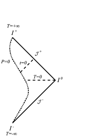
Figure 2: Penrose Diagram for the spacetime in Example 2. We have take $y$ fixed and suppressed the $y$-axis. The only singularity is of $P=0$ type. The lines $t=0$ and $T=0$ are also drawn.

8 Scalar-Field Spacetimes

8.1 Solutions with one spacelike Killing vector

We now find the general solution to 2+1 gravity with a massless scalar-field source under the assumption that there is one spacelike Killing vector. The metric takes the following form:

$${\rm d}s^{2}=-2A(u,v){\rm d}u{\rm d}v+C^{2}(u,v){\rm d}y^{2}.$$

We can transform this to $t,x$ coordinates by defining $u=(t+x)/\sqrt{2}$, $v=(t-x)/\sqrt{2}$. We assume a scalar field source, $\phi=\phi(u,v)$, with energy momentum tensor: $T_{ab}=\partial_{a}\phi\partial_{b}\phi-\tfrac{1}{2}g_{ab}(\partial\phi)^{2}$ where $\phi$ satisfies the conservation equation

$$\square\phi=0.$$

With these prescriptions the $(yu)$ and $(yv)$ components of Einstein equations are satisfied trivially, and the $(yy)$ component requires $C_{,uv}=0$, the general solution of which is:

$$C(u,v)=f(v)+g(u)$$

We also define $D(u,v)=f(v)-g(u)$, and move from $(u,v)$ to $(C,D)$ coordinates. By making different choices of $f(v)$ and $g(u)$ we can arrange that either: $\partial_{a}C$ is spacelike and $\partial_{a}D$ is timelike, or $\partial_{a}D$ is spacelike and $\partial_{a}C$ is time-like, or both $\partial_{a}C$ and $\partial_{a}D$ are null. In terms of $C$ and $D$ the $\phi$ wave equation reads:

$$\phi_{,DD}=\phi_{,CC}+\phi_{,C}/C.$$

This is just the wave-equation in cylindrical polar coordinates with axial and azimuthal symmetry (with $D$ playing the role of the usual time coordinate and $C$ of the radial coordinate). We can solve this in terms of Bessel functions.

$$\phi=\int_{-\infty}^{\infty}{\rm d}kA(k)\left(\cos(\sqrt{k}D)+B(k)\sin(\sqrt{k}D)\right)\left(J_{0}(\sqrt{k}C)+E(k)Y_{0}(\sqrt{k}C)\right),$$

where $A(k),B(k),E(k)\in{\mathbb{C}}$ are arbitrary and $J_{0}$ and $Y_{0}$ are zero-order Bessel functions of the first and second kind respectively. Finally, we solve the equations for $A$ to give:

$$\ln\left(\frac{A}{f^{\prime}(v)g^{\prime}(u)}\right)=2C\int_{D_{0}(C)}^{D}{\rm d}D^{\prime}\phi_{,C}\phi_{,D}+F(C)$$

where

$$F(C)=\int_{C_{0}}^{C}{\rm d}C^{\prime}C^{\prime}\left(\phi_{,C}^{2}+\phi_{,D}^{2}\right)|_{D=D_{0}(C^{\prime})}.$$

Boundary conditions for $\phi$ are need to specify the solution further.

8.2 PP-wave spacetimes

In 2+1 spacetimes the metric for a scalar-field PP-wave spacetime can be written in the form:

$${\rm d}s^{2}=H(u,x){\rm d}u^{2}+2{\rm d}u{\rm d}v+{\rm d}x^{2}.$$

The Einstein equations read $R_{uu}=-1/2H_{,xx}=\kappa(\phi_{,u})^{2}$ and $R_{ab}=0$ otherwise; this implies $\phi=\phi(u)$, where $\phi(u)$ is arbitrary. Solving for $H,$ we find:

$$H=A(u)+B(u)x-\kappa(\phi^{\prime}(u))^{2}~{}x^{2},$$

where $A(u)$ and $B(u)$ can both be freely specified. It can be checked that in 2+1 dimensions these are the only perfect-fluid solutions (they are equivalent to an irrotational $p=\rho$ fluid) that are compatible with the PP-wave metric ansatz given above. Indeed, we find that the only permitted choices of energy-momentum tensor must satisfy $T_{uu}\neq HT$ and $T_{ab}=Tg_{ab}$ otherwise. We find similar PP-wave solutions by considering the 2+1 Einstein-Maxwell equations. Up to gauge transformations, all the solutions are of the form $A_{u}=A_{v}=0$, and $A_{x}=\phi(u)$ for the electromagnetic potential, with $\phi(u)$ arbitrary and $H(u,x)$ as given above. The only non-vanishing components of $F_{ab}$ are $F_{ux}=-F_{xu}=\phi_{,u}(u).$

9 Discussion

Whereas the general cosmological solutions of the 3+1 dimensional Einstein equations are intractably complicated and likely dominated by non-integrability, the structure of the theory in 2+1 offers the possibility of making considerable progress towards finding the general solution in several interesting situations. This fact, together with our current perception that quantum field theory fits more naturally in three rather than four dimensions, has motivated the study of Einstein’s theory in 3-dimensional spacetimes.

In this article we employed covariant and first-order formalism techniques to study the properties of general relativity in three dimensions. The covariant approach provided an irreducible decomposition of the relativistic equations and allowed for a mathematically compact and physically transparent description of their properties. Using this information we reviewed the kinematical, dynamical and geometrical features of 3-dimensional spacetimes and identified the special features that distinguish them from the standard 3+1 models. These include the key role of the isotropic pressure as the sole contributor to the gravitational mass of the system and the fact that vorticity never increases with time. We also reviewed the 3-d analogues of the spatially homogeneous and isotropic FRW models and investigated their stability against linear perturbations. We found that, unlike their conventional counterparts, dust-dominated 3-d homogeneous and isotropic spacetimes are stable under shear and vorticity distortions and (neutrally) stable against disturbances in their density distribution. The latter reflects the vanishing of the total gravitational mass in 3-dimensional dust models, which ensures the absence of linear Jeans-type instabilities. In addition to isotropic spacetimes, we also looked at 3-dimensional anisotropic models providing Kasner-like solutions for the case of pressure-free matter and generalising Gödel’s universe to three dimensions. The covariant formalism allowed us to carry out these analyses by a study of the kinematic variables characterising the expansion of the universe. The absence of both electric and magnetic Weyl curvature components in three dimensions considerably simplifies the analysis. We then specialised further to the case of a pressureless matter source. In addition to being physically realistic, this assumption produces a significant further simplification of the cosmological field equations in three-dimensional spacetimes. We were able to find the general cosmological solutions of the theory in the case where the matter was comoving. No symmetry assumptions were made. We then considered the fully general pressureless fluid system with non-comoving velocities. We were able to solve the system in the case where one spatial velocity component was zero whilst the other was non-zero. This allowed us to carry out an asymptotic study, close to and far from singularities, of an inhomogeneous cosmology with rotation, expansion and shear. All the singularities arising in these solutions were classified using the different criteria of strength introduced by Krolak and Tipler. We were able to provide a simple transformation which generalised all the solutions we found with vanishing cosmological constant into new solutions with non-zero cosmological constant. Finally, we considered scalar-field metric with one Killing vector and found all the PP-wave solutions in 2+1 dimensional universes.

These investigations suggestion a number of problems for further study. Exact solutions in the cases with non-zero isotropic and anisotropic pressure remain to be investigated. In the case of zero pressure, we have analysed the problem of the general solution of the three-dimensional Einstein equations into a well-defined system of partial differential equations. We have solved for the case with comoving velocities and a single non-comoving velocity but the problem remains to find the general solution of the equations when both non-comoving fluid velocities are present.

Acknowledgement

D. Shaw is supported by the PPARC.

References

- [1] Giddings S, Abbott J and Kuchar K 1984 Gen. Rel. Grav. 16 751
- [2] Barrow J D, Burd A B and Lancaster D 1986 Class. Quantum Grav. 3 551
- [3] Staruszkiewicz A 1963 Acta. Phys. Polonica 24 734
- [4] Gott J R and Alpert M 1984 Gen. Rel. Grav. 16 751
- [5] Deser S, Jackiw R and t’Hooft G 1984 Ann. Phys. NY 152 220
- [6] Deser S and Jackiw R 1984 Ann. Phys. NY 140 372
- [7] Deser S and Mazur P 1985 Class. Quantum Grav. 2 L51
- [8] Deser S 1985 in Relativity, Cosmology, Topological Mass and SUGR ed C Aragone (Singapore: World Scientific)
- [9] Bañados M, Teitelboim C and Zanelli J 1992 Phys. Rev. Lett. 69 1849
- [10] Clement G 1976 Nucl. Phys. B 114 437
- [11] Clement G 1984 Gen. Rel. Grav. 16 477
- [12] Clement G 1985 Int. J. Theor. Phys. 24 267
- [13] Garcia A A and Campuzano C 2003 Phys. Rev. D 67 064014
- [14] Ida D 2000 Phys. Rev. Lett. 85 3758
- [15] Vilenkin A 1981 Phys. Rev. D 24 2082
- [16] Gott J R 1985 Astrophys. J. 288 422
- [17] Kaiser N and Stebbins A 1984 Nature 310 391
- [18] Hiscock W A 1985 Phys. Rev. D 31 3288
- [19] Carlip S 1998 Quantum Gravity in (2+1) dimensions (Cambridge: Cambridge UP)
- [20] Collas P 1977 Amer. J. Phys. 45 833
- [21] Garcia A A, Cataldo M and del Campo S 2003 Phys. Rev. D 68 124022
- [22] Kriele M 1997 Class. Quantum Grav. 14 153
- [23] Ross S F and Mann R B 1993 Phys. Rev. D 47 3319
- [24] Gutti S 2005 Class. Quantum Grav. 22 3223
- [25] Witten E 1988 Nucl. Phys. B 311 46
- [26] Szekeres P 1975 Comm. Math. Phys. 41 55
- [27] Barrow J D and Stein-Schabes J 1984 Phys. Lett. A 103 315
- [28] Vermeil H 1917 Nachr. Ges. Wiss. Gottingen 334
- [29] Cartan E 1922 J. Math. Pure Appl. 1 141
- [30] Weyl H 1921 Space, Time, Matter (Berlin: Springer)
- [31] Eisenhart L P 1949 Riemannian Geometry (Princeton: Princeton University Press)
- [32] Stephani H 2004 Relativity (Cambridge: Cambridge University Press)
- [33] Ehlers J 2002 Gen. Rel. Grav. 34 2171
- [34] Ellis G F R and van Elst H 1999 in Theoretical and Observational Cosmology Ed M Lachiéze-Rey (Dordrecht: Kluwer) p 1
- [35] Ellis G F R 1973 in Cargèse Lectures in Physics vol VI ed E Schatzmann (New York: Gordon and Breach) p 1
- [36] Barrow J D 1977 Mon. Not. Roy. astr. Soc. 179 47P
- [37] Ellis G F R and Bruni M 1989 Phys. Rev. D 40 1804
- [38] Gödel K 1949 Rev. Mod. Phys. 21 447
- [39] Ozsváth I and Schücking E 2003 Am. J. Phys. 71 801
- [40] Hawking S W and Ellis G F R 1973 The Large Scale Structure of Spacetime (Cambridge: Cambridge University Press)
- [41] Barrow J D and Tsagas C G 2004 Class. Quantum Grav. 21 1773
- [42] Rooman M and Spindel Ph 1998 Class. Quantum Grav. 15 3241
- [43] Debnath U, Chakraborty S and Barrow J D 2004 Gen. Rel. Grav. 36 231
- [44] Clarke C J S and Królak, A 1985 J. Geom. Phys. 2 127
- [45] Tipler F J 1977 Phys. Lett. A 67 8