About Starobinsky Inflation

Abstract

It is believed that soon after the Planck era, space time should have a semi-classical nature. According to this, the escape from General Relativity theory is unavoidable. Two geometric counter-terms are needed to regularize the divergences which come from the expected value. These counter-terms are responsible for a higher derivative metric gravitation. Starobinsky idea was that these higher derivatives could mimic a cosmological constant. In this work it is considered numerical solutions for general Bianchi I anisotropic space-times in this higher derivative theory. The approach is “experimental” in the sense that there is no attempt to an analytical investigation of the results. It is shown that for zero cosmological constant $\Lambda=0$, there are sets of initial conditions which form basins of attraction that asymptote Minkowski space. The complement of this set of initial conditions form basins which are attracted to some singular solutions. It is also shown, for a cosmological constant $\Lambda>0$ that there are basins of attraction to a specific de Sitter solution. This result is consistent with Starobinsky’s initial idea. The complement of this set also forms basins that are attracted to some type of singular solution. Because the singularity is characterized by curvature scalars, it must be stressed that the basin structure obtained is a topological invariant, i.e., coordinate independent.

I Introduction

The semi-classical theory consider the back reaction of quantum fields in a classical geometric background. It began about forty years ago with De Witt DeWitt , and since then, its consequences and applications are still under research, see for example Hu .

Different of the usual Einstein-Hilbert action, the predicted gravitational action allows differential equations with fourth order derivatives, which is called the full theory DeWitt , see also liv .

There are several problems connected to the full theory which prove that it is not consistent with our expectation of the present day physical world, see Simon and references therein. In this work, Simon and Parker-Simon suggest a perturbative approach which is very interesting.

The full higher order theory was previously studied by Starobinsky S , and more recently, also by Shapiro, Pelinson and others Shapiro . Starobinsky idea was that the higher order terms could mimic a cosmological constant. In Shapiro only the homogeneous and isotropic space time is studied.

The full theory with four time derivatives is addressed, which apparently was first investigated in Tomita’s article berkin for general Bianchi I spaces. They found that the presence of anisotropy contributes to the formation of the singularity. Berkin’s work shows that a quadratic Weyl theory is less stable than a quadratic Riemann scalar $R^{2}$. Barrow and Hervik found exact and analytic solutions for anisotropic quadratic gravity with $\Lambda>0$ that do not approach a de Sitter space time. In that article Barrow and Hervik discuss Bianchi types $II$ and $VI_{h}$ and also a very interesting stability criterion concerning small anisotropies. There is also a recent article by Clifton and Barrow in which Kasner type solutions are addressed. H. J. Schmidt does a recent and very interesting review of higher order gravity theories in connection to cosmology hjs .

On the other hand, numerical investigations of initial conditions, was already addressed in Einstein’s theory of gravitation for the homogeneous Bianchi IX solutions. Basin of attraction to asymptotic solutions, and the fractal nature of the basin boundary are strong indications that the early stages of the Universe were very chaotic, according to Einstein’s theory, see for example cornish .

For general anisotropic Bianchi I homogeneous space times, the full theory reduces to a system of nonlinear ordinary differential equations. The numerical solutions for this system with derivatives of fourth order in time was previously obtained by us sandro .

In this present work a numerical analysis of initial conditions for this nonlinear system mentioned above, is given.

Only the vacuum energy momentum classical source is considered in the full theory. It should be valid soon after the Planck era in which vacuum classical source seems the most natural condition. The chaotic nature of the singularity is not addressed.

There is not a unique way to totally characterize a singularity. In this numerical investigation, the singularity is defined when $R_{ab}R^{ab}>10^{6}$.

It is found that for zero cosmological constant $\Lambda=0$, there are basins that are attracted to zero, constant $4$-curvature solutions. This proves that according to this theory, there are regions in the space of initial conditions, for which the Minkowski geometry is structurally stable. That is, for considerably anisotropic initial conditions isotropisation occurs, and Minkowski space is obtained asymptotically, without the need for fine tuning.

On the other hand for a nonzero cosmological constant $\Lambda>0$ the basins attract to a specific de Sitter geometry, which is a constant homogeneous, non null $4$-curvature solution. Thus indicating that Starobinsky’s inflation is structurally stable in the above sense.

Also, the complement of the set of initial conditions for the stable, physically accepted solutions, for both cases $\Lambda=0$ and $\Lambda>0$, form basins of attraction to singular, in some sense, Universes. Thus physically acceptable initial conditions evolve in very few Planck times, to Universes with very high curvature scalars. In this sense, this theory certainly is not a complete one.

It should be mentioned that the isotropisation process for non zero cosmological constant is not a peculiarity of these higher derivatives theories. It occurs in ordinary Einstein General Relativity theory. This is proved in the very interesting article wald , where for $\Lambda>0$ all Bianchi models, except for highly positively curved Bianchi IX become asymptotically de Sitter. The remarkable difference between General Relativity theory and this higher derivatives theories is that the isotropisation depends on the initial conditions. Isotropisation is strongly dependent on initial conditions for quadratic curvature theories such as (1).

The following conventions and unit choice are taken $R^{a}_{bcd}=\Gamma^{a}_{bd,c}-...$, $R_{ab}=R^{c}_{acb}$, $R=R^{a}_{a}$, metric signature $-+++$, Latin symbols run from $0-3$, Greek symbols run from $1-3$ and $G=\hbar=c=1$.

II The Model

The Lagrange function is,

$${\cal L}=\sqrt{-g}\left[\Lambda+R+\alpha\left(R^{ab}R_{ab}-\frac{1}{3}R^{2}\right)+\beta R^{2}\right]{}+{\cal L}_{c}\,.$$ (1)

Metric variations in the above action results in

$$E_{ab}=G_{ab}+\left(\beta-\frac{1}{3}\alpha\right)H^{(1)}_{ab}+\alpha H^{(2)}_{ab}-T_{ab}-\frac{1}{2}\Lambda g_{ab},$$ (2)

where

$$H^{(1)}_{ab}=\frac{1}{2}g_{ab}R^{2}-2RR_{ab}+2R_{;ab}-2\square Rg_{ab},$$ (3)

$$H^{(2)}_{ab}=\frac{1}{2}g_{ab}R_{mn}R^{mn}+R_{;ab}-2R^{cn}R_{cbna}-\square R_{ab}-\frac{1}{2}\square Rg_{ab},$$ (4)

$$G_{ab}=R_{ab}-\frac{1}{2}g_{ab}R,$$ (5)

and $T_{ab}$ is the energy momentum source, which comes from the classical part of the Lagrangian ${\cal L}_{c}$. Only vacuum solutions $T_{ab}={\cal L}_{c}=0$ will be considered in this paper since it seems the most natural condition soon after the Planck era.

The covariant divergence of the above tensors are identically zero due their variational definition. The following Bianchi Type I line element is considered

$$ds^{2}=-dt^{2}+[a_{1}(t)]^{2}dx^{2}+[a_{2}(t)]^{2}dy^{2}+[a_{3}(t)]^{2}dz^{2},$$ (6)

which is a general spatially flat and anisotropic space, with proper time $t$. With this line element all the tensors which enter the expressions are diagonal. The substitution of (6) in (2) with $T_{ab}=0$, results for the spatial part of (2), in differential equations of the type

$$\frac{d^{4}}{dt^{4}}a_{1}=f_{1}\left(\frac{d^{3}}{dt^{3}}a_{i},\ddot{a}_{i},\dot{a}_{i},a_{i}\right)$$ (7)

$$\frac{d^{4}}{dt^{4}}a_{2}=f_{2}\left(\frac{d^{3}}{dt^{3}}a_{i},\ddot{a}_{i},\dot{a}_{i},a_{i}\right)$$ (8)

$$\frac{d^{4}}{dt^{4}}a_{3}=f_{3}\left(\frac{d^{3}}{dt^{3}}a_{i},\ddot{a}_{i},\dot{a}_{i},a_{i}\right),$$ (9)

where the functions $f_{i}$ involve the $a_{1},\;a_{2},\;a_{3}$, and their derivatives in a polynomial fashion, see the Appendix A. The very interesting article Noakes shows that the theory which follows from (1) has a well posed initial value problem. This question has some similarities which General Relativity theory since it is necessary to solve the problem of boundary conditions and initial conditions simultaneously. According to Noakes Noakes , once a consistent boundary condition is chosen initially, the time evolution of the system is uniquely specified. In Noakes the differential equations for the metric are written in a form suitable for the application of the theorem of Leray Leray . The numerical solutions of the partial differential equations in (2) are not going to be addressed in this present work.

For homogeneous spaces the differential equations in (2) reduce to non linear ordinary differential equations. Then, instead of going through the general construction given in Noakes , in this particular case, the existence and uniqueness of the solutions of (7)-(9) reduce to the well known problem of existence and uniqueness of solutions of ordinary differential equations. For a proof on local existence and uniqueness of solutions of differential equations see, for instance reedsimon .

Besides the equations (7)-(9), we have the temporal part of (2). To understand the role of this equation we have first to study the covariant divergence of the equation (2),

$$\nabla_{a}E^{ab}=\partial_{a}E^{ab}+\Gamma^{a}_{ac}E^{cb}+\Gamma^{b}_{ac}E^{ac}=0.$$

Remind that the coordinates being used are (6) and that $T_{ab}=0$. Since the differential equations (7)-(9) are solved numerically $E^{\alpha\alpha}\equiv 0,$

$$\partial_{0}E^{00}+\Gamma^{a}_{a0}E^{00}+\Gamma^{0}_{00}E^{00}=0,$$

$$E^{00}(t)\equiv 0,$$ (10)

where $E_{00}$ is the $00$ component of (2). If $E_{00}=0$ initially, it will remain zero at any instant. Therefore the equation $E_{00}$ acts as a constraint on the initial conditions and we use it to test the accuracy of our results.

For a space-like vector $v^{\alpha}$ and a time-like vector $t^{a}=(1,0,0,0)$ tidal forces are given by the geodesic deviation equations

$$t^{a}\nabla_{a}v^{\alpha}=R^{\alpha}_{mn\beta}t^{m}t^{n}v^{\beta}$$

$$t^{a}\nabla_{a}v^{\alpha}=R^{\alpha}_{00\beta}v^{\beta}$$

$$R^{\alpha}_{00\beta}=\delta_{\alpha\beta}\left(\frac{\ddot{a}_{\alpha}}{a_{\alpha}}\right).$$

The theory predicted by (1) is believed to be correct if the tidal forces are less than $1$ in Plank units units,

$$|R^{\alpha}_{0\alpha 0}|\leq 1\;\;\text{(no summation.)}$$ (11)

When this condition is not satisfied, quantum effects could introduce further modifications into (1).

III Analysis of initial conditions

Ordinary differential equations are deterministic in the sense that initial conditions specify the dynamical evolution of the system uniquely.

The interest in the numerical investigation is in the sensibility upon initial conditions. In this work, the system is treated as an exit system.

It is a relatively simple approach in which asymptotic classes of solutions are recognized. The initial conditions are identified with respect to which asymptotic solution the system evolves to ott . For this purpose, holes are cut in the phase space and if the system falls into a specific hole, this specifies the asymptotic class. The closure of the set of initial conditions which asymptotes a given solution is called the basin of attraction.

The presence of basins of attraction is an indication of structural stability, since for many initial conditions, without the need for fine tuning, the same class of asymptotic solution is obtained. It is also a topological invariant, since a smooth coordinate transformation is impossible to modify the Hausdorff dimension of a set ott .

In subsections III.1 and III.2, the differential equations (7)-(9) are numerically solved and the initial conditions are chosen in the following way. All the higher derivatives of the metric set initially to zero

$$\frac{d^{3}}{dt^{3}}a_{\alpha}(t=0)=\ddot{a}_{\alpha}(t=0)=0\;\;\text{and}\;a_{1}(t=0)=a_{2}(t=0)=a_{3}(t=0)=1$$ (12)

The Hubble constants in each direction, Appendix A,

$$H_{1}=\frac{\dot{a}_{1}}{a_{1}}\neq 0,\;\;H_{2}=\frac{\dot{a}_{2}}{a_{2}}\neq,0$$ (13)

together with the Hamiltonian constrain (10) fix the initial value of

$$H_{3}=\frac{\dot{a}_{3}}{a_{3}}.$$ (14)

This value is not unique since eq. (10) in the coordinates (6) form a polynomial of degree $3$ in the first derivatives. For arbitrary initial values for $H_{1}$ and $H_{2}$ there could be at most $3$ real distinct initial values for $H_{3}$. One of these values is chosen. It can be seen that the initial values are consistent with the condition (11), resulting in null tidal forces.

III.1 Stability of Minkowski space

In this subsection the cosmological constant is set to zero $\Lambda=0$. The numerical solutions of (7)-(9) are identified according to their asymptotic classes. In FIG. 1 it is shown the isotropisation process toward Minkowski space.

Figure 1: Numerical solution of (7)-(9), with the initial condition described in eqs. (12)-(14), with $\alpha=1$, $\beta=-1$ and $\Lambda=0$, plotted against time, in Planck units. It can be seen the isotropisation towards Minkowski space.

A singularity for which all the 3 dimensions shrink to zero, with $H_{1}<0$, $H_{2}<0$ and $H_{3}<0$ when $t\rightarrow\infty$ is shown in FIG. 2.

Figure 2: Numerical solution of (7)-(9), with the initial condition described in eqs. (12)-(14), with $\alpha=1$, $\beta=-1$ and $\Lambda=0$, plotted against time, in Planck units. It can be seen the formation of a singularity with $H_{1}<0$ and $H_{2}<0$ and $H_{3}<0$.

In FIG. 3 it is shown a singularity for which one of the dimensions increases, either $H_{1}>0$ or $H_{2}>0$ or $H_{3}>0$ and at least one of the $H$ is negative, when $t\rightarrow\infty$.

Figure 3: Numerical solution of (7)-(9), with the initial condition described in eqs. (12)-(14), with $\alpha=1$, $\beta=-1$ and $\Lambda=0$, plotted against time, in Planck units. It can be seen the formation of a singularity with at least $H_{1}>0$ or $H_{2}>0$ or $H_{3}>0$, and at least one of the $H$ is negative.

In FIG. 4, a black, white or gray point is addressed to a initial condition whether it falls into the classes shown in FIG. 1, FIG. 2 or FIG. 3 respectively.

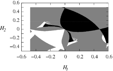
Figure 4: A two dimensional section defined by (12)-(14) and (10), for the phase space of (7)-(9), with $400\times 400$ initial values for $H_{1}$ and $H_{2}$. $\alpha=1$, $\beta=-1$ and $\Lambda=0$. The black regions are the basins of attraction to the Minkowski space. The white and gray regions are initial conditions which asymptote the singularities shown in FIG. 2 and FIG. 3 respectively.

III.2 Stability of de Sitter space

In this subsection a non zero cosmological constant is chosen $\Lambda=0.02$. The map of initial conditions for the differential equations (7)-(9), is almost identical to the last section, except for the black point. Each black point in FIG. 5 corresponds to initial conditions whose solution asymptote a constant $4$ curvature space $R=R_{ab}g^{ab}=-0.04$ shown in FIG. 6.

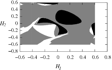
Figure 5: A two dimensional section defined by (12)-(14) and (10), for the phase space of (7)-(9), with $400\times 400$ initial values for $H_{1}$ and $H_{2}$. $\alpha=1$, $\beta=-1$ and $\Lambda=0.02$. The black regions are the basins of attraction to the de Sitter space sown in FIG. 6. The white and gray regions are initial conditions which asymptote the singularities shown in FIG. 2 and FIG. 3 respectively.

In FIG. 6 the time evolution of a black point in FIG. 5 shows the isotropisation process toward a de Sitter, constant curvature solution.

Figure 6: Numerical solution of (7)-(9), with the initial condition described in eqs. (12)-(14), with $\alpha=1$, $\beta=-1$ and $\Lambda=0.02$, plotted against time, in Planck units. It can be seen the isotropisation toward a de Sitter space with $R=R_{ab}g^{ab}=-0.04$.

The basins of attraction to this same de Sitter solution, is an indication of stability in some sense.

IV Conclusions

In the present work it is considered general anisotropic Bianchi I homogeneous space times given by the line element (6). For this line element, the theory given in (1), reduces to a system of ordinary nonlinear differential equations with four time derivatives. This system is numerically investigated. In particular, an analysis of initial conditions is given, which is the interest from the dynamical system point of view. The supposition of a homogeneous Universe is artificial, and still presents a first generalization for its very primordial stages.

Anyway, there is a well known conjecture that dissipative processes can take place in a infinite dynamical system reducing the number of degrees of freedom to just a few. In some sense, this argument reduces the artificiality of the supposition of a homogeneous Universe.

Only the vacuum energy momentum classical source is considered in the full theory. It should be valid soon after the Planck era in which vacuum classical source seems the most natural condition. The chaotic nature of the singularity is not addressed.

There is not a unique way to totally characterize a singularity. In this numerical investigation, the singularity is defined when $R_{ab}R^{ab}>10^{6}$.

It is found that for zero cosmological constant $\Lambda=0$, there are basins that are attracted to zero, constant $4$-curvature solutions. This proves that according to this theory, there are regions in the space of initial conditions, for which the Minkowski geometry is structurally stable. That is, for considerably anisotropic initial conditions isotropisation occurs, and Minkowski space is obtained asymptotically, without the need for fine tuning. The fact that the Minkowski space is an attractor to general Bianchi I spaces must be connected to non linear effects, see Appendix A.

On the other hand for a nonzero cosmological constant $\Lambda>0$ the basins attract to a specific de Sitter solution. That is, constant homogeneous, non null $4$-curvature solutions. Thus reproducing Starobinsky’s idea.

Also, the complement of the set of initial conditions for the stable, physically accepted solutions, for both cases $\Lambda=0$ and $\Lambda>0$, form basins of attraction to singular, in some sense, Universes. Thus physically acceptable initial conditions evolve in very few Planck times, to Universes with very high curvature scalars. In this sense, this theory certainly is not a complete one.

It should be mentioned that the isotropisation process for non zero cosmological constant is not a peculiarity of these higher derivatives theories. It occurs in ordinary Einstein General Relativity theory. This is proved in the very interesting article wald , where for $\Lambda>0$ all Bianchi models, except for highly positively curved Bianchi IX become asymptotically de Sitter. The remarkable difference between General Relativity theory and this higher derivatives theories is that the isotropisation depends on the initial conditions. Isotropisation is strongly dependent on initial conditions for quadratic curvature theories such as (1).

The analytical solutions found by Barrow-Hervik and Clifton-Barrow berkin can be understood as limit sets in the space of solutions of the quadratic theory (1). In particular, Barrow-Hervik found solutions for which isotropisation does not occur. In this present work it is shown that the initial conditions for which isotropistation does not occur, form a set with non zero measure. Every gray point in FIG. 4 and FIG. 5 corresponds to solutions for which isotropisation does not occur.A bifurcation analysis with respect to the parameters space, $\alpha,\;\beta,\;\Lambda$ is beyond the scope of the present work.

Appendix A The differential equations

The following line element is chosen

$$ds^{2}=-dt^{2}+e^{2w_{{1}}(t)}dx^{2}+e^{2w_{{2}}(t)}dy^{2}+e^{2w_{{3}}(t)}dz^{2}.$$

With this choice, the first time derivatives of the functions $w_{{i}}(t)$ are related to the functions $a_{{i}}(t)$ of (6) in the following manner

$$y_{{1}} = \dot{w_{{1}}}=\frac{\dot{a_{{1}}}}{a_{{1}}}$$ (15)

$$y_{{2}} = \dot{w_{{2}}}=\frac{\dot{a_{{2}}}}{a_{{2}}}$$ (16)

$$y_{{3}} = \dot{w_{{3}}}=\frac{\dot{a_{{3}}}}{a_{{3}}}$$ (17)

$$y_{{4}} = \ddot{w_{{1}}}=\frac{\ddot{a_{{1}}}}{a_{{1}}}-\left(\frac{\dot{a_{{1}}}}{a_{{1}}}\right)^{2}$$ (18)

$$y_{{5}} = \ddot{w_{{2}}}=\frac{\ddot{a_{{2}}}}{a_{{2}}}-\left(\frac{\dot{a_{{2}}}}{a_{{2}}}\right)^{2}$$ (19)

$$y_{{6}} = \ddot{w_{{3}}}=\frac{\ddot{a_{{3}}}}{a_{{3}}}-\left(\frac{\dot{a_{{3}}}}{a_{{3}}}\right)^{2}$$ (20)

$$y_{{7}} = \frac{d^{3}}{dt^{3}}w_{{1}}=\frac{1}{a_{{1}}}\frac{d^{3}}{dt^{3}}a_{{1}}-\frac{\dot{a_{{1}}}}{a_{{1}}}\left(3\frac{\ddot{a_{{1}}}}{a_{{1}}}-2\left(\frac{\dot{a_{{1}}}}{a_{{1}}}\right)^{2}\right)$$ (21)

$$y_{{8}} = \frac{d^{3}}{dt^{3}}w_{{2}}=\frac{1}{a_{{2}}}\frac{d^{3}}{dt^{3}}a_{{2}}-\frac{\dot{a_{{2}}}}{a_{{2}}}\left(3\frac{\ddot{a_{{2}}}}{a_{{2}}}-2\left(\frac{\dot{a_{{2}}}}{a_{{2}}}\right)^{2}\right)$$ (22)

$$y_{{9}} = \frac{d^{3}}{dt^{3}}w_{{3}}=\frac{1}{a_{{3}}}\frac{d^{3}}{dt^{3}}a_{{3}}-\frac{\dot{a_{{3}}}}{a_{{3}}}\left(3\frac{\ddot{a_{{3}}}}{a_{{3}}}-2\left(\frac{\dot{a_{{3}}}}{a_{{3}}}\right)^{2}\right).$$ (23)

The differential equations for the quadratic theory with the classical source $T_{ab}=0$, (2), are equivalent to

$$\frac{d^{4}}{dt^{4}}w_{{1}} = {\frac{11}{9}}\,y_{{3}}y_{{1}}{y_{{2}}}^{2}-{\frac{19}{9}}\,y_{{3}}y_{{2}}{y_{{1}}}^{2}+{\frac{11}{9}}\,y_{{2}}y_{{1}}{y_{{3}}}^{2}+5/3\,y_{{1}}y_{{2}}y_{{5}}-13/3\,y_{{1}}y_{{2}}y_{{4}}$$ (24)

$$-13/3\,y_{{1}}y_{{3}}y_{{4}}+1/9\,y_{{1}}y_{{6}}y_{{2}}+5/3\,y_{{1}}y_{{3}}y_{{6}}+2/3\,y_{{2}}y_{{3}}y_{{6}}-{\frac{14}{9}}\,y_{{2}}y_{{3}}y_{{4}}+2/3\,y_{{2}}y_{{3}}y_{{5}}$$

$$+1/9\,y_{{1}}y_{{3}}y_{{5}}-\left({\frac{1}{108}}\,y_{{3}}y_{{1}}{y_{{2}}}^{2}+{\frac{1}{108}}\,y_{{3}}y_{{2}}{y_{{1}}}^{2}+{\frac{1}{108}}\,y_{{2}}y_{{1}}{y_{{3}}}^{2}+{\frac{1}{54}}\,y_{{1}}y_{{6}}y_{{2}}\right.$$

$$\left.+{\frac{1}{54}}\,y_{{2}}y_{{3}}y_{{4}}+{\frac{1}{54}}\,y_{{1}}y_{{3}}y_{{5}}-{\frac{1}{108}}\,y_{{5}}y_{{4}}-{\frac{1}{108}}\,y_{{6}}y_{{4}}-{\frac{1}{108}}\,y_{{6}}y_{{5}}+1/27\,{y_{{1}}}^{2}{y_{{2}}}^{2}\right.$$

$$\left.+1/27\,{y_{{1}}}^{2}{y_{{3}}}^{2}+1/27\,{y_{{2}}}^{2}{y_{{3}}}^{2}-1/36\,{y_{{3}}}^{3}y_{{1}}-1/36\,{y_{{1}}}^{3}y_{{2}}-1/36\,{y_{{1}}}^{3}y_{{3}}-1/36\,{y_{{2}}}^{3}y_{{1}}\right.$$

$$\left.-1/36\,{y_{{3}}}^{3}y_{{2}}-1/36\,{y_{{2}}}^{3}y_{{3}}-{\frac{1}{54}}\,y_{{1}}y_{{7}}-{\frac{1}{54}}\,y_{{2}}y_{{8}}-{\frac{1}{54}}\,y_{{3}}y_{{9}}+{\frac{1}{108}}\,y_{{8}}y_{{1}}+{\frac{1}{108}}\,y_{{2}}y_{{7}}\right.$$

$$\left.+{\frac{1}{108}}\,y_{{9}}y_{{1}}+{\frac{1}{108}}\,y_{{9}}y_{{2}}+{\frac{1}{108}}\,y_{{3}}y_{{8}}+{\frac{1}{108}}\,{y_{{4}}}^{2}+{\frac{1}{108}}\,{y_{{5}}}^{2}+{\frac{1}{108}}\,{y_{{6}}}^{2}+{\frac{1}{108}}\,{y_{{2}}}^{4}\right.$$

$$\left.+{\frac{1}{108}}\,{y_{{3}}}^{4}-{\frac{1}{54}}\,{y_{{1}}}^{2}y_{{4}}-{\frac{1}{54}}\,{y_{{2}}}^{2}y_{{5}}-{\frac{1}{54}}\,{y_{{3}}}^{2}y_{{6}}+{\frac{1}{108}}\,y_{{3}}y_{{7}}+{\frac{1}{108}}\,{y_{{1}}}^{4}\right)\alpha{\beta}^{-1}$$

$$-\left(-1/18\,y_{{6}}-1/18\,y_{{5}}+1/6\,\Lambda-1/18\,{y_{{3}}}^{2}-1/36\,y_{{3}}y_{{2}}-1/18\,{y_{{2}}}^{2}-1/18\,y_{{4}}-1/36\,y_{{3}}y_{{1}}\right.$$

$$\left.-1/18\,{y_{{1}}}^{2}-1/36\,y_{{2}}y_{{1}}\right)/(G\beta)-{\frac{11}{9}}\,y_{{5}}y_{{4}}-{\frac{11}{9}}\,y_{{6}}y_{{4}}+1/9\,y_{{6}}y_{{5}}-{\frac{5}{18}}\,{y_{{1}}}^{2}{y_{{2}}}^{2}-{\frac{5}{18}}\,{y_{{1}}}^{2}{y_{{3}}}^{2}$$

$$+{\frac{7}{18}}\,{y_{{2}}}^{2}{y_{{3}}}^{2}+2/3\,{y_{{3}}}^{3}y_{{1}}-2/3\,{y_{{1}}}^{3}y_{{2}}-2/3\,{y_{{1}}}^{3}y_{{3}}+2/3\,{y_{{2}}}^{3}y_{{1}}-{\frac{22}{9}}\,y_{{1}}y_{{7}}-1/9\,y_{{2}}y_{{8}}$$

$$-1/9\,y_{{3}}y_{{9}}-1/9\,y_{{8}}y_{{1}}-{\frac{16}{9}}\,y_{{2}}y_{{7}}-1/9\,y_{{9}}y_{{1}}+2/9\,y_{{9}}y_{{2}}+2/9\,y_{{3}}y_{{8}}-{\frac{29}{18}}\,{y_{{4}}}^{2}$$

$$-{\frac{5}{18}}\,{y_{{5}}}^{2}-{\frac{5}{18}}\,{y_{{6}}}^{2}-{\frac{5}{18}}\,{y_{{2}}}^{4}-{\frac{5}{18}}\,{y_{{3}}}^{4}-1/9\,{y_{{1}}}^{2}y_{{4}}-{\frac{7}{9}}\,{y_{{2}}}^{2}y_{{5}}-{\frac{7}{9}}\,{y_{{3}}}^{2}y_{{6}}-{\frac{16}{9}}\,y_{{3}}y_{{7}}$$

$$-4/3\,y_{{5}}{y_{{1}}}^{2}-4/3\,y_{{6}}{y_{{1}}}^{2}+1/3\,y_{{6}}{y_{{2}}}^{2}+1/3\,{y_{{3}}}^{2}y_{{5}}-\left(\left(4/3\,y_{{3}}y_{{1}}{y_{{2}}}^{2}-8/3\,y_{{3}}y_{{2}}{y_{{1}}}^{2}\right.\right.$$

$$\left.\left.+4/3\,y_{{2}}y_{{1}}{y_{{3}}}^{2}-4\,y_{{1}}y_{{2}}y_{{5}}-4\,y_{{1}}y_{{2}}y_{{4}}-4\,y_{{1}}y_{{3}}y_{{4}}-4/3\,y_{{1}}y_{{6}}y_{{2}}-4\,y_{{1}}y_{{3}}y_{{6}}+8\,y_{{2}}y_{{3}}y_{{6}}\right.\right.$$

$$\left.\left.+8/3\,y_{{2}}y_{{3}}y_{{4}}+8\,y_{{2}}y_{{3}}y_{{5}}-4/3\,y_{{1}}y_{{3}}y_{{5}}-4/3\,y_{{5}}y_{{4}}-4/3\,y_{{6}}y_{{4}}+8/3\,y_{{6}}y_{{5}}-8/3\,{y_{{1}}}^{2}{y_{{2}}}^{2}\right.\right.$$

$$\left.\left.-8/3\,{y_{{1}}}^{2}{y_{{3}}}^{2}+16/3\,{y_{{2}}}^{2}{y_{{3}}}^{2}-4\,{y_{{1}}}^{3}y_{{2}}-4\,{y_{{1}}}^{3}y_{{3}}+4\,{y_{{3}}}^{3}y_{{2}}+4\,{y_{{2}}}^{3}y_{{3}}-8/3\,y_{{1}}y_{{7}}\right.\right.$$

$$\left.\left.+4/3\,y_{{2}}y_{{8}}+4/3\,y_{{3}}y_{{9}}-8/3\,y_{{8}}y_{{1}}+4/3\,y_{{2}}y_{{7}}-8/3\,y_{{9}}y_{{1}}+4/3\,y_{{9}}y_{{2}}+4/3\,y_{{3}}y_{{8}}-8/3\,{y_{{4}}}^{2}\right.\right.$$

$$\left.\left.+4/3\,{y_{{5}}}^{2}+4/3\,{y_{{6}}}^{2}+4/3\,{y_{{2}}}^{4}+4/3\,{y_{{3}}}^{4}-{\frac{32}{3}}\,{y_{{1}}}^{2}y_{{4}}+16/3\,{y_{{2}}}^{2}y_{{5}}+16/3\,{y_{{3}}}^{2}y_{{6}}\right.\right.$$

$$\left.\left.+4/3\,y_{{3}}y_{{7}}-4\,y_{{5}}{y_{{1}}}^{2}-4\,y_{{6}}{y_{{1}}}^{2}+4\,y_{{6}}{y_{{2}}}^{2}+4\,{y_{{3}}}^{2}y_{{5}}-8/3\,{y_{{1}}}^{4}\right)\beta+\left(-1/3\,{y_{{3}}}^{2}-1/3\,y_{{5}}\right.\right.$$

$$\left.\left.-1/3\,{y_{{2}}}^{2}-2/3\,y_{{3}}y_{{2}}-1/3\,y_{{6}}+2/3\,{y_{{1}}}^{2}+2/3\,y_{{4}}+1/3\,y_{{2}}y_{{1}}+1/3\,y_{{3}}y_{{1}}\right)/G\right){\alpha}^{-1}$$

$$+{\frac{7}{18}}\,{y_{{1}}}^{4}$$

$$\frac{d^{4}}{dt^{4}}w_{{2}} = -{\frac{19}{9}}\,y_{{3}}y_{{1}}{y_{{2}}}^{2}+{\frac{11}{9}}\,y_{{3}}y_{{2}}{y_{{1}}}^{2}+{\frac{11}{9}}\,y_{{2}}y_{{1}}{y_{{3}}}^{2}-13/3\,y_{{1}}y_{{2}}y_{{5}}+5/3\,y_{{1}}y_{{2}}y_{{4}}+2/3\,y_{{1}}y_{{3}}y_{{4}}$$

$$+1/9\,y_{{1}}y_{{6}}y_{{2}}+2/3\,y_{{1}}y_{{3}}y_{{6}}+5/3\,y_{{2}}y_{{3}}y_{{6}}+1/9\,y_{{2}}y_{{3}}y_{{4}}-13/3\,y_{{2}}y_{{3}}y_{{5}}-{\frac{14}{9}}\,y_{{1}}y_{{3}}y_{{5}}$$

$$-\left({\frac{1}{108}}\,y_{{3}}y_{{1}}{y_{{2}}}^{2}+{\frac{1}{108}}\,y_{{3}}y_{{2}}{y_{{1}}}^{2}+{\frac{1}{108}}\,y_{{2}}y_{{1}}{y_{{3}}}^{2}+{\frac{1}{54}}\,y_{{1}}y_{{6}}y_{{2}}+{\frac{1}{54}}\,y_{{2}}y_{{3}}y_{{4}}\right.$$ (25)

$$\left.+{\frac{1}{54}}\,y_{{1}}y_{{3}}y_{{5}}-{\frac{1}{108}}\,y_{{5}}y_{{4}}-{\frac{1}{108}}\,y_{{6}}y_{{4}}-{\frac{1}{108}}\,y_{{6}}y_{{5}}+1/27\,{y_{{1}}}^{2}{y_{{2}}}^{2}+1/27\,{y_{{1}}}^{2}{y_{{3}}}^{2}\right.$$

$$\left.+1/27\,{y_{{2}}}^{2}{y_{{3}}}^{2}-1/36\,{y_{{3}}}^{3}y_{{1}}-1/36\,{y_{{1}}}^{3}y_{{2}}-1/36\,{y_{{1}}}^{3}y_{{3}}-1/36\,{y_{{2}}}^{3}y_{{1}}-1/36\,{y_{{3}}}^{3}y_{{2}}\right.$$

$$\left.-1/36\,{y_{{2}}}^{3}y_{{3}}-{\frac{1}{54}}\,y_{{1}}y_{{7}}-{\frac{1}{54}}\,y_{{2}}y_{{8}}-{\frac{1}{54}}\,y_{{3}}y_{{9}}+{\frac{1}{108}}\,y_{{8}}y_{{1}}+{\frac{1}{108}}\,y_{{2}}y_{{7}}+{\frac{1}{108}}\,y_{{9}}y_{{1}}\right.$$

$$\left.+{\frac{1}{108}}\,y_{{9}}y_{{2}}+{\frac{1}{108}}\,y_{{3}}y_{{8}}+{\frac{1}{108}}\,{y_{{4}}}^{2}+{\frac{1}{108}}\,{y_{{5}}}^{2}+{\frac{1}{108}}\,{y_{{6}}}^{2}+{\frac{1}{108}}\,{y_{{2}}}^{4}+{\frac{1}{108}}\,{y_{{3}}}^{4}\right.$$

$$\left.-{\frac{1}{54}}\,{y_{{1}}}^{2}y_{{4}}-{\frac{1}{54}}\,{y_{{2}}}^{2}y_{{5}}-{\frac{1}{54}}\,{y_{{3}}}^{2}y_{{6}}+{\frac{1}{108}}\,y_{{3}}y_{{7}}+{\frac{1}{108}}\,{y_{{1}}}^{4}\right)\alpha{\beta}^{-1}-\left(-1/18\,y_{{6}}\right.$$

$$\left.-1/18\,y_{{5}}+1/6\,\Lambda-1/18\,{y_{{3}}}^{2}-1/36\,y_{{3}}y_{{2}}-1/18\,{y_{{2}}}^{2}-1/18\,y_{{4}}-1/36\,y_{{3}}y_{{1}}\right.$$

$$\left.-1/18\,{y_{{1}}}^{2}-1/36\,y_{{2}}y_{{1}}\right)/(G\beta)-{\frac{11}{9}}\,y_{{5}}y_{{4}}+1/9\,y_{{6}}y_{{4}}-{\frac{11}{9}}\,y_{{6}}y_{{5}}-{\frac{5}{18}}\,{y_{{1}}}^{2}{y_{{2}}}^{2}$$

$$+{\frac{7}{18}}\,{y_{{1}}}^{2}{y_{{3}}}^{2}-{\frac{5}{18}}\,{y_{{2}}}^{2}{y_{{3}}}^{2}+2/3\,{y_{{1}}}^{3}y_{{2}}-2/3\,{y_{{2}}}^{3}y_{{1}}+2/3\,{y_{{3}}}^{3}y_{{2}}-2/3\,{y_{{2}}}^{3}y_{{3}}$$

$$-1/9\,y_{{1}}y_{{7}}-{\frac{22}{9}}\,y_{{2}}y_{{8}}-1/9\,y_{{3}}y_{{9}}-{\frac{16}{9}}\,y_{{8}}y_{{1}}-1/9\,y_{{2}}y_{{7}}+2/9\,y_{{9}}y_{{1}}-1/9\,y_{{9}}y_{{2}}$$

$$-{\frac{16}{9}}\,y_{{3}}y_{{8}}-{\frac{5}{18}}\,{y_{{4}}}^{2}-{\frac{29}{18}}\,{y_{{5}}}^{2}-{\frac{5}{18}}\,{y_{{6}}}^{2}+{\frac{7}{18}}\,{y_{{2}}}^{4}-{\frac{5}{18}}\,{y_{{3}}}^{4}-{\frac{7}{9}}\,{y_{{1}}}^{2}y_{{4}}-1/9\,{y_{{2}}}^{2}y_{{5}}$$

$$-{\frac{7}{9}}\,{y_{{3}}}^{2}y_{{6}}+2/9\,y_{{3}}y_{{7}}+1/3\,y_{{6}}{y_{{1}}}^{2}-4/3\,y_{{6}}{y_{{2}}}^{2}-{\frac{5}{18}}\,{y_{{1}}}^{4}-4/3\,{y_{{2}}}^{2}y_{{4}}+1/3\,{y_{{3}}}^{2}y_{{4}}$$

$$-\left(\left(-8/3\,y_{{3}}y_{{1}}{y_{{2}}}^{2}+4/3\,y_{{3}}y_{{2}}{y_{{1}}}^{2}+4/3\,y_{{2}}y_{{1}}{y_{{3}}}^{2}-4\,y_{{1}}y_{{2}}y_{{5}}-4\,y_{{1}}y_{{2}}y_{{4}}+8\,y_{{1}}y_{{3}}y_{{4}}\right.\right.$$

$$\left.\left.-4/3\,y_{{1}}y_{{6}}y_{{2}}+8\,y_{{1}}y_{{3}}y_{{6}}-4\,y_{{2}}y_{{3}}y_{{6}}-4/3\,y_{{2}}y_{{3}}y_{{4}}-4\,y_{{2}}y_{{3}}y_{{5}}+8/3\,y_{{1}}y_{{3}}y_{{5}}-4/3\,y_{{5}}y_{{4}}\right.\right.$$

$$\left.\left.+8/3\,y_{{6}}y_{{4}}-4/3\,y_{{6}}y_{{5}}-8/3\,{y_{{1}}}^{2}{y_{{2}}}^{2}+16/3\,{y_{{1}}}^{2}{y_{{3}}}^{2}-8/3\,{y_{{2}}}^{2}{y_{{3}}}^{2}+4\,{y_{{3}}}^{3}y_{{1}}\right.\right.$$

$$\left.\left.+4\,{y_{{1}}}^{3}y_{{3}}-4\,{y_{{2}}}^{3}y_{{1}}-4\,{y_{{2}}}^{3}y_{{3}}+4/3\,y_{{1}}y_{{7}}-8/3\,y_{{2}}y_{{8}}+4/3\,y_{{3}}y_{{9}}+4/3\,y_{{8}}y_{{1}}-8/3\,y_{{2}}y_{{7}}\right.\right.$$

$$\left.\left.+4/3\,y_{{9}}y_{{1}}-8/3\,y_{{9}}y_{{2}}+4/3\,y_{{3}}y_{{8}}+4/3\,{y_{{4}}}^{2}-8/3\,{y_{{5}}}^{2}+4/3\,{y_{{6}}}^{2}-8/3\,{y_{{2}}}^{4}+4/3\,{y_{{3}}}^{4}\right.\right.$$

$$\left.\left.+16/3\,{y_{{1}}}^{2}y_{{4}}-{\frac{32}{3}}\,{y_{{2}}}^{2}y_{{5}}+16/3\,{y_{{3}}}^{2}y_{{6}}+4/3\,y_{{3}}y_{{7}}+4\,y_{{6}}{y_{{1}}}^{2}-4\,y_{{6}}{y_{{2}}}^{2}+4/3\,{y_{{1}}}^{4}\right.\right.$$

$$\left.\left.-4\,{y_{{2}}}^{2}y_{{4}}+4\,{y_{{3}}}^{2}y_{{4}}\right)\beta+\left(-1/3\,{y_{{3}}}^{2}+2/3\,y_{{5}}+2/3\,{y_{{2}}}^{2}+1/3\,y_{{3}}y_{{2}}-1/3\,y_{{6}}\right.\right.$$

$$\left.\left.-1/3\,{y_{{1}}}^{2}-1/3\,y_{{4}}+1/3\,y_{{2}}y_{{1}}-2/3\,y_{{3}}y_{{1}}\right)/G\right){\alpha}^{-1}$$

$$\frac{d^{4}}{dt^{4}}w_{{3}} = {\frac{11}{9}}\,y_{{3}}y_{{1}}{y_{{2}}}^{2}+{\frac{11}{9}}\,y_{{3}}y_{{2}}{y_{{1}}}^{2}-{\frac{19}{9}}\,y_{{2}}y_{{1}}{y_{{3}}}^{2}+2/3\,y_{{1}}y_{{2}}y_{{5}}+2/3\,y_{{1}}y_{{2}}y_{{4}}$$

$$+5/3\,y_{{1}}y_{{3}}y_{{4}}-{\frac{14}{9}}\,y_{{1}}y_{{6}}y_{{2}}-13/3\,y_{{1}}y_{{3}}y_{{6}}-13/3\,y_{{2}}y_{{3}}y_{{6}}+1/9\,y_{{2}}y_{{3}}y_{{4}}+5/3\,y_{{2}}y_{{3}}y_{{5}}$$

$$+1/9\,y_{{1}}y_{{3}}y_{{5}}-\left({\frac{1}{108}}\,y_{{3}}y_{{1}}{y_{{2}}}^{2}+{\frac{1}{108}}\,y_{{3}}y_{{2}}{y_{{1}}}^{2}+{\frac{1}{108}}\,y_{{2}}y_{{1}}{y_{{3}}}^{2}+{\frac{1}{54}}\,y_{{1}}y_{{6}}y_{{2}}\right.$$

$$\left.+{\frac{1}{54}}\,y_{{2}}y_{{3}}y_{{4}}+{\frac{1}{54}}\,y_{{1}}y_{{3}}y_{{5}}-{\frac{1}{108}}\,y_{{5}}y_{{4}}-{\frac{1}{108}}\,y_{{6}}y_{{4}}-{\frac{1}{108}}\,y_{{6}}y_{{5}}+1/27\,{y_{{1}}}^{2}{y_{{2}}}^{2}\right.$$

$$\left.+1/27\,{y_{{1}}}^{2}{y_{{3}}}^{2}+1/27\,{y_{{2}}}^{2}{y_{{3}}}^{2}-1/36\,{y_{{3}}}^{3}y_{{1}}-1/36\,{y_{{1}}}^{3}y_{{2}}-1/36\,{y_{{1}}}^{3}y_{{3}}-1/36\,{y_{{2}}}^{3}y_{{1}}\right.$$

$$\left.-1/36\,{y_{{3}}}^{3}y_{{2}}-1/36\,{y_{{2}}}^{3}y_{{3}}-{\frac{1}{54}}\,y_{{1}}y_{{7}}-{\frac{1}{54}}\,y_{{2}}y_{{8}}-{\frac{1}{54}}\,y_{{3}}y_{{9}}+{\frac{1}{108}}\,y_{{8}}y_{{1}}+{\frac{1}{108}}\,y_{{2}}y_{{7}}\right.$$

$$\left.+{\frac{1}{108}}\,y_{{9}}y_{{1}}+{\frac{1}{108}}\,y_{{9}}y_{{2}}+{\frac{1}{108}}\,y_{{3}}y_{{8}}+{\frac{1}{108}}\,{y_{{4}}}^{2}+{\frac{1}{108}}\,{y_{{5}}}^{2}+{\frac{1}{108}}\,{y_{{6}}}^{2}+{\frac{1}{108}}\,{y_{{2}}}^{4}\right.$$

$$\left.+{\frac{1}{108}}\,{y_{{3}}}^{4}-{\frac{1}{54}}\,{y_{{1}}}^{2}y_{{4}}-{\frac{1}{54}}\,{y_{{2}}}^{2}y_{{5}}-{\frac{1}{54}}\,{y_{{3}}}^{2}y_{{6}}+{\frac{1}{108}}\,y_{{3}}y_{{7}}+{\frac{1}{108}}\,{y_{{1}}}^{4}\right)\alpha{\beta}^{-1}-\left(-1/18\,y_{{6}}\right.$$

$$\left.-1/18\,y_{{5}}+1/6\,\Lambda-1/18\,{y_{{3}}}^{2}-1/36\,y_{{3}}y_{{2}}-1/18\,{y_{{2}}}^{2}-1/18\,y_{{4}}-1/36\,y_{{3}}y_{{1}}\right.$$

$$\left.-1/18\,{y_{{1}}}^{2}-1/36\,y_{{2}}y_{{1}}\right)/(G\beta)+1/9\,y_{{5}}y_{{4}}-{\frac{11}{9}}\,y_{{6}}y_{{4}}-{\frac{11}{9}}\,y_{{6}}y_{{5}}+{\frac{7}{18}}\,{y_{{1}}}^{2}{y_{{2}}}^{2}-{\frac{5}{18}}\,{y_{{1}}}^{2}{y_{{3}}}^{2}$$

$$-{\frac{5}{18}}\,{y_{{2}}}^{2}{y_{{3}}}^{2}-2/3\,{y_{{3}}}^{3}y_{{1}}+2/3\,{y_{{1}}}^{3}y_{{3}}-2/3\,{y_{{3}}}^{3}y_{{2}}+2/3\,{y_{{2}}}^{3}y_{{3}}-1/9\,y_{{1}}y_{{7}}-1/9\,y_{{2}}y_{{8}}$$

$$-{\frac{22}{9}}\,y_{{3}}y_{{9}}+2/9\,y_{{8}}y_{{1}}+2/9\,y_{{2}}y_{{7}}-{\frac{16}{9}}\,y_{{9}}y_{{1}}-{\frac{16}{9}}\,y_{{9}}y_{{2}}-1/9\,y_{{3}}y_{{8}}-{\frac{5}{18}}\,{y_{{4}}}^{2}-{\frac{5}{18}}\,{y_{{5}}}^{2}$$

$$-{\frac{29}{18}}\,{y_{{6}}}^{2}-{\frac{5}{18}}\,{y_{{2}}}^{4}+{\frac{7}{18}}\,{y_{{3}}}^{4}-{\frac{7}{9}}\,{y_{{1}}}^{2}y_{{4}}-{\frac{7}{9}}\,{y_{{2}}}^{2}y_{{5}}-1/9\,{y_{{3}}}^{2}y_{{6}}-1/9\,y_{{3}}y_{{7}}+1/3\,y_{{5}}{y_{{1}}}^{2}$$

$$-4/3\,{y_{{3}}}^{2}y_{{5}}-\left(\left(4/3\,y_{{3}}y_{{1}}{y_{{2}}}^{2}+4/3\,y_{{3}}y_{{2}}{y_{{1}}}^{2}-8/3\,y_{{2}}y_{{1}}{y_{{3}}}^{2}+8\,y_{{1}}y_{{2}}y_{{5}}+8\,y_{{1}}y_{{2}}y_{{4}}\right.\right.$$

$$\left.\left.-4\,y_{{1}}y_{{3}}y_{{4}}+8/3\,y_{{1}}y_{{6}}y_{{2}}-4\,y_{{1}}y_{{3}}y_{{6}}-4\,y_{{2}}y_{{3}}y_{{6}}-4/3\,y_{{2}}y_{{3}}y_{{4}}-4\,y_{{2}}y_{{3}}y_{{5}}-4/3\,y_{{1}}y_{{3}}y_{{5}}\right.\right.$$

$$\left.\left.+8/3\,y_{{5}}y_{{4}}-4/3\,y_{{6}}y_{{4}}-4/3\,y_{{6}}y_{{5}}+16/3\,{y_{{1}}}^{2}{y_{{2}}}^{2}-8/3\,{y_{{1}}}^{2}{y_{{3}}}^{2}-8/3\,{y_{{2}}}^{2}{y_{{3}}}^{2}\right.\right.$$

$$\left.\left.-4\,{y_{{3}}}^{3}y_{{1}}+4\,{y_{{1}}}^{3}y_{{2}}+4\,{y_{{2}}}^{3}y_{{1}}-4\,{y_{{3}}}^{3}y_{{2}}+4/3\,y_{{1}}y_{{7}}+4/3\,y_{{2}}y_{{8}}-8/3\,y_{{3}}y_{{9}}+4/3\,y_{{8}}y_{{1}}\right.\right.$$

$$\left.\left.+4/3\,y_{{2}}y_{{7}}+4/3\,y_{{9}}y_{{1}}+4/3\,y_{{9}}y_{{2}}-8/3\,y_{{3}}y_{{8}}+4/3\,{y_{{4}}}^{2}+4/3\,{y_{{5}}}^{2}-8/3\,{y_{{6}}}^{2}+4/3\,{y_{{2}}}^{4}\right.\right.$$

$$\left.\left.-8/3\,{y_{{3}}}^{4}+16/3\,{y_{{1}}}^{2}y_{{4}}+16/3\,{y_{{2}}}^{2}y_{{5}}-{\frac{32}{3}}\,{y_{{3}}}^{2}y_{{6}}-8/3\,y_{{3}}y_{{7}}+4\,y_{{5}}{y_{{1}}}^{2}-4\,{y_{{3}}}^{2}y_{{5}}\right.\right.$$

$$\left.\left.+4/3\,{y_{{1}}}^{4}+4\,{y_{{2}}}^{2}y_{{4}}-4\,{y_{{3}}}^{2}y_{{4}}\right)\beta+\left(2/3\,{y_{{3}}}^{2}-1/3\,y_{{5}}-1/3\,{y_{{2}}}^{2}+1/3\,y_{{3}}y_{{2}}+2/3\,y_{{6}}\right.\right.$$

$$\left.\left.-1/3\,{y_{{1}}}^{2}-1/3\,y_{{4}}-2/3\,y_{{2}}y_{{1}}+1/3\,y_{{3}}y_{{1}}\right)/G\right){\alpha}^{-1}-{\frac{5}{18}}\,{y_{{1}}}^{4}+1/3\,{y_{{2}}}^{2}y_{{4}}$$

$$-4/3\,{y_{{3}}}^{2}y_{{4}}$$ (26)

References

- (1) B. S. De Witt, The Dynamical Theory of Groups and Fields, Gordon and Breach, New York, (1965).
- (2) B. L. Hu, E. Verdaguer, Living Rev. Rel. 7, 3, (2004).
- (3) A. A. Grib, S. G. Mamayev and V. M. Mostepanenko, Vacuum Quantum Effects in Strong Fields, Friedmann Laboratory Publishing, St. Petersburg (1994), N. D. Birrel and P. C. W. Davies, Quantum Fields in Curved Space, Cambridge University Press, Cambridge (1982).
- (4) J. Z. Simon, Phys. Rev. D, 45, 1953 (1992); L. Parker and J. Z. Simon, ibid., 47,1339 (1993).
- (5) A. A. Starobinsky, Phys. Lett. 91B, 99 (1980);Ya. B. Zeldovich and A. A. Starobinsky, Sov. Phys. - JETP(USA), 34, 1159 (1972), V. N. Lukash and A. A. Starobinsky, Sov. Phys. - JEPT(USA), 39, 742 (1974).
- (6) A. M. Pelinson, I. L. Shapiro, F. I. Takakura, Nucl. Phys. B648, 417, (2003); J. C. Fabris, A. M. Pelinson, I. L. Shapiro, Nucl.Phys.B597 539 (2001), Erratum-ibid. B602 644 (2001); J. C. Fabris, A. M. Pelinson, I. L. Shapiro, Nucl.Phys.Proc.Suppl. 95 78 (2001); J. C. Fabris, A. M. Pelinson, I. L. Shapiro, Grav.Cosmol.6 59 (2000)
- (7) A. L. Berkin, Phys. Rev. D 44, p. 1020 (1991), J. D. Barrow and S. Hervik, Phys. Rev. D 73, 023007 (2006), K. Tomita et al. Prog. of Theor Phys 60 (2), p403 (1978), T. Clifton and J. D. Barrow, Class. Quant. Grav. 23, 2951 (2006).
- (8) H. J. Schmidt, gr-qc/0602017, (2006).
- (9) G. Francisco and G. E. A. Matsas, Gen. Rel. Grav. 20, 1047 (1988); N. J. Cornish and J. J. Levin Phys. Rev. Lett. 78, 998 (1997); N. J. Cornish and J. J. Levin Phys. Rev. D 55, 7489 (1997).
- (10) S. P. Vitenti and D. Müller, gr-qc/0604127 (2006).
- (11) R. M. Wald, Phys. Rev. D 28, 2118 (1983).
- (12) D. E. Noakes, J. Math. Phys. 24, 1846 (1983).
- (13) J. Leray, Hyperbolic Differential Equations, Institute for Advanced Study, Princeton, NJ (1953).
- (14) M. Reed and B. Simon, Methods of Modern Mathematical Physics I: Functional Analysis, Academic Press, NY, p. 153 (1972).
- (15) S. Bleher, C. Grebogi, E. Ott, R. Brown Phys. Rev. A 38, 930 (1988); C. Grebogi, E. Ott and J. A. Yorke Phys. Rev. Lett. 50, 935 (1983); E. Ott Chaos in Dynamical Systems, Second Edition , Cambridge University Press (2002).