Static Ricci-flat 5-manifolds admitting the 2-sphere

Abstract

We examine, in a purely geometrical way, static Ricci-flat 5-manifolds admitting the 2-sphere and an additional hypersurface-orthogonal Killing vector. These are widely studied in the literature, from different physical approaches, and known variously as the Kramer - Gross - Perry - Davidson - Owen solutions. The 2-fold infinity of cases that result are studied by way of new coordinates (which are in most cases global) and the cases likely to be of interest in any physical approach are distinguished on the basis of the nakedness and geometrical mass of their associated singularities. It is argued that the entire class of solutions has to be considered unstable about the exceptional solutions: the black string and soliton cases. Any physical theory which admits the non-exceptional solutions as the external vacuua of a collapsing object has to accept the possibility of collapse to zero volume leaving behind the weakest possible, albeit naked, geometrical singularities at the origin. Finally, it is pointed out that these types of solutions generalize, in a straightforward way, to higher dimensions.

I Introduction

Wide importance is now attached to the study of higher dimensional spaces as the arena of physical phenomena. However, as we go beyond spacetime, the topological possibilities introduce a new dimension to the difficulty of attaching physical significance to various manifolds. Even at five dimensions, asymptotically flat stationary vacuum black holes are not unique in the sense that horizons of topology $S^{1}\times S^{2}$ er in addition to $S^{3}$ mp are now known. However, in the simpler static case, it is known that asymptotically flat static vacuum black holes are unique flat and given by the Tangherlini generalization of the Schwarzschild vacuum tangherlini . These uniqueness properties suggest that these solutions represent the natural generalization of the Schwarzschild spacetime. However, these are not the only asymptotically flat quasi-static vacua which can be considered “spherically symmetric”.

Here we are concerned with 5-manifolds which admit only the 2- sphere (unlike the Tangherlini vacua which admit the 3-sphere) and, in addition, two hypersurface orthogonal Killing vectors at least one of which is assumed timelike. These spaces are widely studied in the literature from various physical approaches wesson but the approach used here is purely geometrical and the results therefore applicable to any physical approach. The only assumption made, aside from the symmetries stated, is

$${}^{(5)}R_{ab}=0$$ (1)

where ${}^{(5)}R_{ab}$ is the 5-dimensional Ricci tensor.

II Symmetries

To set the notation let $\xi$ represent a Killing vector field,

$$\nabla_{(a}\;\xi_{\;b)}=0$$ (2)

and if, for the coordinate $x^{i}$ is adapted( $\xi^{a}=\delta^{a}_{x^{i}}$), represent the associated field by ${}_{x^{i}}\xi$. If, in addition to (2), $\xi$ also satisfies the hypersurface orthogonality condition

$$\xi_{\;[a}\nabla_{\;b}\;\xi_{\;c]}=0,$$ (3)

write the field as $\tilde{\xi}$. The traditional definition of a static region of spacetime is one which admits a timelike $\tilde{\xi}$. This terminology is also used here and we distinguish the adapted coordinate $t$ via timelike ${}_{t}\tilde{\xi}$. The spaces considered here admit an additional hypersurface orthogonal Killing vector and we distinguish the adapted coordinate $w$ via ${}_{w}\tilde{\xi}$. (Any internal properties of $w$ are therefore of no concern.) In addition to these symmetries we assume 2-dimensional spherical symmetry. That is, the spaces can be decomposed as

$$ds^{2}=ds^{2}_{3}+\mathcal{R}^{2}d\Omega^{2}_{2}$$ (4)

where

$$d\Omega^{2}_{2}\equiv d\theta^{2}+\sin(\theta)^{2}d\phi^{2}$$ (5)

so that we also have the Killing field

$$\xi^{\theta}=c_{1}\cos(\phi)+c_{2}\sin(\phi)$$ (6)

and

$$\xi^{\phi}=c_{3}-\cot(\theta)(c_{1}\sin(\phi)-c_{2}\cos(\phi))$$ (7)

where $c_{1},\;c_{2}$ and $c_{3}$ are non-zero constants and the other components of this $\xi$ are zero. This $\xi$ of course includes ${}_{\phi}\tilde{\xi}$. Here $\mathcal{R}$ is independent of $t,w,\theta$ and $\phi$ and if $\mathcal{R}=0$ we refer to this circumstance as an “origin”.

III Parameter Space of Solutions

With the foregoing symmetries it follows that (1) is satisfied by

$$ds^{2}=Ah^{\alpha}dw^{2}+Bh^{\delta}dt^{2}+\frac{dr^{2}+S^{2}d\Omega^{2}_{2}}{fS^{4}}$$ (8)

where $A$ and $B$ are non-zero constants, $\alpha$ and $\delta$ are constants (not both zero), $h=h(r)$ (assumed monotone),

$$f=Ch^{\alpha+\delta-2}(h^{\prime})^{2}$$ (9)

where $C$ is a non-zero constant, ${}^{{}^{\prime}}\equiv d/dr$ and

$$S(r)=\pm\frac{h^{(2\sqrt{\epsilon\nu}-1)/(2\sqrt{\epsilon\nu})}(\epsilon h^{1/\sqrt{\epsilon\nu}}-\nu)}{h^{{}^{\prime}}}$$ (10)

where $\epsilon$ and $\nu$ are constants restricted by the relation

$$\alpha^{2}+\delta^{2}+\alpha\delta=\frac{1}{\epsilon\nu}\equiv\frac{1}{\lambda^{2}}>0.$$ (11)

To view (8) as static we take $B=-1$ (unless otherwise noted) and to view (8) as an augmentation of spacetime (with signature +2) we take $C>0$. We retain both signs of $A$ and so allow the doubly static cases $A=B=-1$. Note that the forms of $f$ and $S$ remain unchanged under the interchange $\alpha\leftrightarrow\delta$ leon . The reason for this symmetry here is that the adapted coordinates $w$ and $t$ are (prior to setting $B=-1$) interchangeable.

Since the magnitude of $A$ (and of course $B$) can be absorbed into the scale of $w$ (and $t$), the form (8) would appear at first sight to admit three independently specified constants, in addition to $C$, via (11). This, however, is not the case as we can, without loss in generality, set

$$\epsilon=\nu=\frac{1}{2}$$ (12)

thus simplifying (10) to the form

$$S(r)=\pm\frac{h^{2}-1}{2h^{{}^{\prime}}}.$$ (13)

This is shown in the Appendix. There are then only two specifiable parameters ($C$ and $\alpha$ or $\delta$ subject to (11) with (12)).

IV Generating explicit solutions

Clearly the form (8) allows an infinite number of representations given a monotone function $h(r)$ subject to the reality of the resultant metric coefficients. Another approach is to assume a form for $S(r)$ and solve the differential equation (13). For example, if we set $S(r)=r$ we obtain the solution given by Gross and Perry grossandperry and Davidson and Owen davidson . Similarly, setting $S(r)=\sinh(r)$ we obtain the solution given recently by Millward millward . These representations are discussed in a more direct way below.

Whereas (13) can be solved exactly for a wide variety of choices for $S(r)$, we can of course use $h$ as a coordinate and view (13) as the required coordinate transformation. With $h$ as a coordinate (8) takes the simple form

$$ds^{2}=Ah^{\alpha}dw^{2}+Bh^{\delta}dt^{2}+\frac{dh^{2}+\mathcal{S}^{2}d\Omega^{2}_{2}}{\mathsf{f}\mathcal{S}^{4}}$$ (14)

where now

$$\mathsf{f}=\mathsf{f}(h)=(2C)^{2}h^{\alpha+\delta-2},$$ (15)

$$\mathcal{S}=\mathcal{S}(h)=\pm\frac{(h^{2}-1)}{2},$$ (16)

and

$$\alpha^{2}+\delta^{2}+\alpha\delta=4.$$ (17)

The coefficient in (45) has been redefined for convenience. An important aspect of what follows is the distinction, on geometrical grounds, of various members of the solution locus (17).

Other representations

Whereas the from (14) is convenient (and as is shown below, complete in most cases), coordinate transformations bring the spaces into more familiar forms. For example, with the transformation

$$h=\sqrt{1-\frac{1}{Cr}}$$ (18)

we obtain the form given by Kramer kramer . Similarly, with the transformation

$$h=\left(\frac{4Cr+1}{4Cr-1}\right)$$ (19)

we obtain form given by given by Gross and Perry grossandperry (the notation (here to there) is related by $\delta\rightarrow-2/\alpha,\alpha\rightarrow-2\beta/\alpha$, and $C\rightarrow 1/4m$) and by Davidson and Owen davidson (the notation (here to there) is related by $\delta\rightarrow-2\epsilon k,\alpha\rightarrow 2\epsilon$, and $C\rightarrow a/4$). The solution given recently by Millward millward is a very special case. It is given by

$$h=e^{\sqrt{3}b}$$ (20)

with $\alpha=\delta=\frac{2}{\sqrt{3}}$ and $C^{2}=\frac{1}{3M^{2}}$.

V Properties of the solutions (14)

In this section we study the geometric properties of the solutions (14). The various solutions are distinguished in Figure 1 via the parameters $\alpha$ and $\delta$. First, however, we discuss the interchange symmetry associated with the solution locus (17).

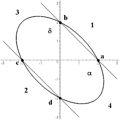
Figure 1: The solution locus $\alpha^{2}+\delta^{2}+\alpha\delta=4$ (ellipse) along with $\alpha+\delta=2$ (top line) and $\alpha+\delta=-2$ (bottom line). Quadrants are indicated for convenience. These quadrants do not include the exceptional solutions $a=(2,0),b=(0,2),c=(-2,0)$ and $d=(0,-2)$ which are discussed separately as they have very distinct properties.

Interchange Symmetry

The solution locus (17) is obviously invariant to the interchange $(\alpha,\delta)\leftrightarrow(-\alpha,-\delta)$ wesson1 . To see why, consider the coordinate transformation

$$h=\frac{1}{r}.$$ (21)

Under the transformation (21) we obtain (14) but with $h\rightarrow r$, $\alpha\rightarrow-\alpha$, and $\delta\rightarrow-\delta$. Moreover, in terms of Figure 1, we have the quadrant interchanges $1\leftrightarrow 2$ and $3\leftrightarrow 4,$ along with the point interchanges $a\leftrightarrow c$ and $b\leftrightarrow d$. As a result, the form (14) duplicates all distinct classes of solutions. As a matter of convenience we continue with this form here but with knowledge of this duplicity.

Distinguishing The Constant $C$

Before the properties of the solutions (14) are discussed in terms of the parameters $\alpha$ and $\delta$, it is useful to review the general nature of the constant $C$ as it is quite distinct from $\alpha$ and $\delta$. This is similar to (the reciprocal of) the “mass” in the four-dimensional Schwarzschild vacuum as one might well guess from the other representations discussed above and as we explain in detail below. To see this let $ds^{2}$ represent the 4 dimensional Schwarzschild vacuum (of mass $m$) and subject this to a conformal transformation

$$ds^{2}\rightarrow\Phi^{2}ds^{2}$$ (22)

where $\Phi$ is a constant. This, of course, preserves Ricci flatness (in any dimension). It is easy to show that under the transformation (22)

$$m\rightarrow\pm|\Phi|m.$$ (23)

It is clear from the form (14) then that $1/C$ plays a role similar to $m$ (using the freedom in the scale of $w$ and $t$). The parameters $\alpha$ and $\delta$, however, distinguish the solutions (14) in a rather different way as we now examine.

Origins

As explained above, we refer to $\mathcal{R}^{2}=0$ as an origin. From (14) we have

$$\mathcal{R}^{2}=\frac{h^{2-\alpha-\delta}}{C^{2}(h^{2}-1)^{2}}$$ (24)

so that in all cases $\lim_{h\rightarrow 1^{\pm}}\mathcal{R}^{2}\rightarrow\infty$. Moreover, $\mathcal{R}$ has a minimum ($>0$) at

$$h^{2}=\frac{\alpha+\delta-2}{\alpha+\delta+2}$$ (25)

which restricts the minima to quadrants $1$ and $2$ of Figure 1. In quadrant $1$ the minima occur for $h\in(0,1)$ and in quadrant $2$ they exist for $h\in(1,\infty)$. For the exceptional solutions $a$ and $b$ clearly $\mathcal{R}^{2}=1/C^{2}(h^{2}-1)^{2}$ and for the exceptional solutions $c$ and $d$, $\mathcal{R}^{2}=h^{4}/C^{2}(h^{2}-1)^{2}$. Properties of $\mathcal{R}^{2}$ are summarized in Tables 1 and 2.

Table 1: “Regular” solutions

$h$	1	2	3 and 4
$\in(0,1)$	$\mathcal{R}^{2}\rightarrow\infty$	$\mathcal{R}^{2}\rightarrow 0$	$\mathcal{R}^{2}\rightarrow 0$
$\rightarrow 0^{+}$	$W\rightarrow\infty$	$W\rightarrow\infty$	$W\rightarrow\infty$
	$SL^{*}$	$TL$	$N$ and $TL$
	$m\rightarrow\pm\infty$	$m\rightarrow 0$	$m\rightarrow\pm\infty$
$\rightarrow 1^{\pm}$	$\mathcal{R}^{2}\rightarrow\infty$	$\mathcal{R}^{2}\rightarrow\infty$	$\mathcal{R}^{2}\rightarrow\infty$
	$W\rightarrow 0$	$W\rightarrow 0$	$W\rightarrow 0$
$\in(1,\infty)$	$\mathcal{R}^{2}\rightarrow 0$	$\mathcal{R}^{2}\rightarrow\infty$	$\mathcal{R}^{2}\rightarrow 0$
$\rightarrow\infty$	$W\rightarrow\infty$	$W\rightarrow\infty$	$W\rightarrow\infty$
	$TL$	$SL^{*}$	$TL$ and $N$
	$m\rightarrow 0$	$m\rightarrow\pm\infty$	$m\rightarrow\pm\infty$

Table 2: “Exceptional” solutions

$h$	$a$ and $b$	$c$ and $d$
$\in(0,1)$	$\mathcal{R}^{2}\rightarrow 1/C^{2}$	$\mathcal{R}^{2}\rightarrow 0$
$\rightarrow 0^{+}$	$W\rightarrow 12C^{4}$	$W\rightarrow\infty$
		$TL$ and $TL$
$\rightarrow 1^{\pm}$	$\mathcal{R}^{2}\rightarrow\infty$	$\mathcal{R}^{2}\rightarrow\infty$
	$W\rightarrow 0$	$W\rightarrow 0$
$\in(1,\infty)$	$\mathcal{R}^{2}\rightarrow 0$	$\mathcal{R}^{2}\rightarrow 1/C^{2}$
$\rightarrow\infty$	$W\rightarrow\infty$	$W\rightarrow 12C^{4}$
	$TL$ and $TL$

Weyl Invariant

For the spaces (14) there is only one independent invariant derivable from the Riemann tensor without differentiation and this can be taken to be ${}^{(5)}C_{abcd}$${}^{(5)}C^{abcd}\equiv W$ where ${}^{(5)}C_{abcd}$ is the 5-dimensional Weyl tensor. This is given by weyl

$$W=\frac{3h^{2(\alpha+\delta-4)}(h^{2}-1)^{6}C^{4}\mathcal{H}}{32}$$ (26)

where

$$\mathcal{H}\equiv(8-\alpha\delta)\left((8+\alpha\delta)(h^{4}+1)+4(\alpha+\delta)(h^{4}-1)\right)$$

$$+2h^{2}\alpha^{2}\delta^{2}.\;\;\;\;\;\$$ (27)

First note that for the exceptional cases $a$ and $b$

$$W=12(h^{2}-1)^{6}C^{4},$$ (28)

and for the exceptional cases $c$ and $d$

$$W=\frac{12(h^{2}-1)^{6}C^{4}}{h^{12}}.$$ (29)

In all cases

$$\lim_{h\rightarrow 1^{\pm}}W\rightarrow 0.$$ (30)

Moreover,

$$\lim_{h\rightarrow 0}W\rightarrow\infty$$ (31)

except for the exceptional cases $a$ and $b$ for which $\lim_{h\rightarrow 0}W\rightarrow 12C^{4}$ and

$$\lim_{h\rightarrow\infty}W\rightarrow\infty$$ (32)

except for the exceptional cases $c$ and $d$ for which $\lim_{h\rightarrow\infty}W\rightarrow 12C^{4}$. The limit (31) shows that in all but the two cases indicated, the solution (14) is singular at $h=0$. Similarly, the limit (32) shows that in all but the other two cases indicated, the solution (14) is singular as $h\rightarrow\infty$. The properties discussed above are summarized in Tables 1 and 2.

Local Asymptotic flatness

Since, as shown above,

$$\lim_{h\rightarrow 1^{\pm}}\mathcal{R}^{2}\rightarrow\infty,$$ (33)

and since

$$\lim_{h\rightarrow 1^{\pm}}\;^{(5)}R_{ab}^{\;\;\;cd}\rightarrow 0,$$ (34)

where ${}^{(5)}R_{ab}^{\;\;\;cd}$ is the 5-dimensional Riemann tensor, all solutions are (locally) asymptotically flat for $h\rightarrow 1^{\pm}$.

Subspaces $w$ $=$ constant

In any subspace $w=$ constant it follows from (14) that ${}^{(4)}R_{ab}=0$ only for $\alpha=0$, that is a subspace of the exceptional solutions $b$ and $d$. These are “black string” solutions string . Moreover, $C^{2}=1/4m^{2}$ where $m$ is the usual Schwarzschild mass (as we discuss further below). With the aide of Table 2 we see that for the solution $b$, $h\in(0,1)$ covers the static part of the spacetime with $m>0$ and all of the spacetime with $m<0$ for $h\in(1,\infty)$. Similarly, the solution $d$ with $h\in(1,\infty)$ covers the static part of the spacetime with $m>0$ and all of the spacetime with $m<0$ for $h\in(0,1)$. (In an analogous way, we can consider any subspace $t=$ constant with $A=-1$ and interchange $a$ for $b$, $c$ for $d$ and $\alpha$ for $\delta$ in the foregoing. The exceptional cases $a$ and $c$ we call “soliton” solutions grossandperry .)

Nature of the Singularities

Hypersurfaces of constant $h$ in subspaces of constant $w$ can be categorized by way of the trajectories they contain. Here we distinguish the spacelike ($SL,2\mathcal{L}>0$), timelike ($TL,2\mathcal{L}<0$) and null ($N,2\mathcal{L}=0$) cases where $2\mathcal{L}\equiv\;^{(5)}v_{a}\;^{(5)}v^{a}$ and ${}^{(5)}v^{a}=(0,\dot{t},0,\dot{\theta},\dot{\phi)}$ is tangent to a curve in the hypersurface (${}^{.}\equiv d/d\lambda$, where $\lambda$ is any parameter that distinguishes events along the curve). From (14) we find

$$2\mathcal{L}=-h^{\delta}\dot{t}^{2}+\mathcal{R}^{2}(\dot{\theta}^{2}+\sin(\theta)^{2}\dot{\phi}^{2}).$$ (35)

The nature of the singularities thus categorized are summarized in Tables 1 and 2 where $SL^{*}$ means $N$ if exactly radial ($\dot{\theta}=\dot{\phi}=0$).

Null Geodesics

Write the momenta conjugate to ${}_{t}\tilde{\xi},\;_{w}\tilde{\xi}$ and ${}_{\phi}\tilde{\xi}$ as $p_{t},\;p_{w}$ and $p_{\phi}$ and define the constants of motion $\mathcal{C}_{w}\equiv p_{w}/p_{t}$ and $\mathcal{C}_{\phi}\equiv p_{\phi}/p_{t}$. The null geodesic equation now follows as

$$\dot{h}^{2}=f\mathcal{S}^{4}\left(\frac{1}{h^{\delta}}-\frac{\mathcal{C}_{w}^{2}}{Ah^{\alpha}}-\frac{\mathcal{C}_{\phi}^{2}}{\mathcal{R}^{2}}\right)$$ (36)

where ${}^{.}\equiv d/d\lambda$ for a suitably scaled affine parameter $\lambda$ and without loss in generality we have set $\theta=\pi/2$. In general then the singularities discussed above are “directional” in their visibility as there exist turning points in $h$. In the “radial” case $\mathcal{C}_{w}=\mathcal{C}_{\phi}=0$ we have

$$\dot{h}^{2}=h^{\alpha-2}(h^{2}-1)^{4}.$$ (37)

Whereas (37) can be integrated in terms of special functions, this integration is not needed. We simply observe that there are no turning points on $h\in(0,1)$ or on $h\in(1,\infty)$. As a result, only in the exceptional solutions $a$ and $b$ on $h\in(0,1)$ and $c$ and $d$ on $h\in(1,\infty)$ are the forms (14) incomplete and also free of naked singularities in the ranges given naked .

Static Extensions

It is clear from Table 2 that the exceptional solutions $a$ and $b$ are incomplete on $h\in(0,1)$ and the exceptional solutions $c$ and $d$ are incomplete on $h\in(1,\infty)$. Since there is no geometrical reason to terminate these cases, we consider here simple static extensions. In these cases (but clearly not in general) we can consider $h<0$. First note that the discussion on asymptotic flatness given above extends to $h\rightarrow-1^{\pm}$ in these cases. Moreover, the results given in Table 2 extend directly to $h<0$. It follows then that the cases $a$ and $b$ on $h\in(-1,1)$ and $c$ and $d$ on $h\in(-1,-\infty)\bigcup(1,\infty)$ are singular-free. However, as we know from the 4-dimensional case, these static extensions can be incomplete.

Non-Static Extensions

For the black string solutions $b$ and $d$ we can write

$$ds^{2}=Adw^{2}+d\tilde{s}^{2}$$ (38)

where $d\tilde{s}^{2}$ is any regular completion of the Schwarzschild manifold so the space is no longer static via ${}_{t}\tilde{\xi}$. If $A=-1$ the space remains static via ${}_{w}\tilde{\xi}$. Similarly, if $A=-1$ for the soliton solutions $a$ and $c$ we can write

$$ds^{2}=-dt^{2}+d\tilde{s}^{2}$$ (39)

where again $d\tilde{s}^{2}$ is any regular completion of the Schwarzschild manifold so the space is no longer static via ${}_{w}\tilde{\xi}$ but remains static via ${}_{t}\tilde{\xi}$. Of course, the past spacelike singularities in $d\tilde{s}^{2}$ render these solutions also nakedly singular, but in a way quite unlike the foregoing.

Geometrical Mass

Not all singularities can be considered equally serious. Here we define the geometrical mass associated with spherical symmetry in order to classify the singularities discussed above. Define the quantity $m$ via the sectional curvature of the two-sphere mass ,

$$m\equiv\frac{{}^{(5)}R_{\theta\phi}^{\;\;\;\;\theta\phi}g_{\theta\theta}^{3/2}}{2}.$$ (40)

(In 4 dimensions the well known effective gravitational mass of spherically symmetric spacetimes is given by (40) with ⁽⁵⁾ replaced by ⁽⁴⁾.)

It follows from (14) that masswesson

$$m=-\frac{((\alpha+\delta)^{2}+4)(h^{2}-1)+4(\alpha+\delta)(h^{2}+1)}{32Ch^{(\alpha+\delta+2)/2}},$$ (41)

so that in all cases

$$\lim_{h\rightarrow 1}m=-\frac{\alpha+\delta}{4C}.$$ (42)

However, only in the exceptional solutions is $m$ a constant and then,

$$m=\pm\frac{1}{2C}.$$ (43)

The properties of $m$ in the other solutions are summarized in Table 1. In what follows we classify the geometrical “strength” of a singularity on the basis of $m$.

VI The View from Above

Most of the foregoing generalizes in a straightforward way to higher dimensions. For example, at dimension 6, introducing another hypersurface-orthogonal Killing vector ${}_{y}\tilde{\xi}$, it follows (retaining the previous notation) that

$$ds^{2}=Ah^{\alpha}dw^{2}+Bh^{\delta}dt^{2}+Dh^{\epsilon}dy^{2}+\frac{dh^{2}+\mathcal{S}^{2}d\Omega^{2}_{2}}{\mathsf{f}\mathcal{S}^{4}},$$ (44)

where $D$ and $\epsilon$ are constants,

$$\mathsf{f}=(2C)^{2}h^{\alpha+\delta+\epsilon-2},$$ (45)

and (16) still holds, satisfies ${}^{(6)}R_{a}^{b}=0$ as long as the parameters remain on the ellipsoid

$$\alpha^{2}+\delta^{2}+\epsilon^{2}+\alpha\delta+\alpha\epsilon+\delta\epsilon=4.$$ (46)

Of particular interest here is the fact that in any subspace $y=$ constant it follows from (44) that ${}^{(5)}R_{a}^{b}=0$ only for $\epsilon=0$. These subspaces are precisely the spaces considered in this paper.

VII Discussion

As the foregoing discussion makes clear, solutions on the locus (17) have quite distinct geometrical properties, and not all of these solutions can be considered equally valid in any physical approach. For example, solutions in the quadrants 3 and 4 have the strongest possible geometrical singularities at the origin ($m$ diverges at $\mathcal{R}=0$), and these singularities are visible throughout the associated spaces for the entire range in $h$. In quadrant 1 for $h\in(0,1)$ and quadrant 2 for $h\in(1,\infty)$ the solutions not only lack an origin, they have the strongest possible geometrical singularities. In contrast, quadrant 1 solutions with $h\in(1,\infty)$ and quadrant 2 solutions with $h\in(0,1)$ have visible but the weakest possible geometrical singularities at the origin ($m\rightarrow 0$). In contrast, the exceptional solutions have quite distinct properties. Solutions $a$ and $b$ with $h\in(1,\infty)$ and solutions $c$ and $d$ with $h\in(0,1)$ have naked singularities at the origin but of intermediate strength ($m$ remains finite deformed ). Only for the solutions $a$ and $b$ with $h\in(0,1)$ and the solutions $c$ and $d$ with $h\in(1,\infty)$ are the coordinates used in (14) incomplete. In these cases singularities in the non-static extensions are obtained. Because of the very distinct properties of the solutions as one covers the solution locus (17), the natural conclusion is that the solution (14) is fundamentally unstable about these exceptional solutions. That is, the properties of the exceptional black string and soliton solutions are unstable to any metric perturbation. In general, if one was to envisage a physical theory in which (14) was the external geometry of an object collapsing to zero volume, quadrant 1 solutions with $h\in(1,\infty)$ (equivalently quadrant 2 solutions with $h\in(0,1)$) would seem to be the natural choice since their properties are stable (away from the exceptional solutions) and have the weakest possible, albeit naked, geometrical singularities at the origin zeromass . Finally, it was pointed out how the spaces considered here can be thought of as subspaces of a higher dimensional Ricci-flat manifold of similar type.

*

Appendix A $\epsilon=\nu=\frac{1}{2}$

In this appendix we prove that we can, without loss in generality, set $\epsilon=\nu=\frac{1}{2}$ in (8) thus simplifying (10) to the form (13). We include $B$ for completeness. Define

$$\bar{\alpha}\equiv 2\lambda\alpha,\;\;\;\bar{\delta}\equiv 2\lambda\delta$$ (47)

so that

$$\bar{\alpha}^{2}+\bar{\delta}^{2}+\bar{\alpha}\bar{\delta}=4.$$ (48)

Next, define $H$ by

$$h\equiv\left(\frac{\nu}{\epsilon}\right)^{\lambda}H^{2\lambda}.$$ (49)

With these definitions (8) transforms as follows:

$$Ah^{\alpha}\rightarrow\bar{A}H^{\bar{\alpha}},\;\;\;Bh^{\delta}\rightarrow\bar{B}H^{\bar{\delta}}$$ (50)

where

$$\bar{A}=A\left(\frac{\nu}{\epsilon}\right)^{\bar{\alpha}/2},\;\;\;\bar{B}=B\left(\frac{\nu}{\epsilon}\right)^{\bar{\delta}/2}$$ (51)

and

$$f\rightarrow\bar{C}H^{\bar{\alpha}+\bar{\delta}-2}(H^{{}^{\prime}})^{2}$$ (52)

where

$$\bar{C}=4\lambda^{2}\left(\frac{\nu}{\epsilon}\right)^{(\bar{\alpha}+\bar{\delta})/2}C$$ (53)

and finally

$$\mathcal{S}\rightarrow\pm\frac{H^{2}-1}{2H^{{}^{\prime}}}.$$ (54)

Thus, with the relabelling $H\rightarrow h$ and the removal of the ${}^{\bar{}}\;\;$, we obtain a space equivalent to the form (8) but with $\epsilon=\nu=\frac{1}{2}$.

References

- (1) Electronic Address: lake@astro.queensu.ca
- (2) R. Emparan and H. S. Reall, Phys. Rev. Lett. 88, 101101 (2002) (hep-th/0110260).
- (3) R. C. Myers and M. J. Perry, Annals Phys. 172, 304 (1986) .
- (4) S. Hwang, Geometriae Dedicata 71, 5 (1998), G. W. Gibbons, D. Ida and T. Shiromizu, Prog. Theor. Phys. Suppl. 148, 284 (2003) arXiv:gr-qc/0203004
- (5) F. R. Tangherlini, Nuovo Cimento 27, 636 (1963). Explicit regular coordinates that cover all of the Tangherlini solutions are given by K. Lake, JCAP 0310 (2003) 007 arXiv:gr-qc/0306073
- (6) See, for example, J. M. Overduin and P. S. Wesson, Phys. Rept. 283 (1997) arXiv:gr-qc/9805018.
- (7) For further discussion of this property see J. Ponce de Leon, Class. Quantum Grav. 23 3043 (2006) arXiv:gr-qc/0512067
- (8) D. J. Gross and M. J. Perry, Nucl. Phys. B 226, 29 (1983). Our use of the term “soliton” here is consistent with this work.
- (9) A. Davidson and D. Owen, Phys. Lett. B 155, 247 (1985).
- (10) R. S. Millward arXiv:gr-qc/0603132
- (11) D. Kramer, Acta Phys. Polon. B2, 807 (1970).
- (12) The significance of this symmetry (along with explained previously) has sometimes been considered obscure. See, for example, P. S. Wesson, Space-Time-Matter (World Scientific, Singapore, 1999).
- (13) This invariant has been given previously in different coordinates (see, for example, the references in wesson ), but to our knowledge the discussion given here is more complete than any given previously. Moreover, the evolution in must be considered along with the geometrical mass as defined below.
- (14) It is well known that the black string solutions are unstable to large-scale perturbations. See R. Gregory, Class. Quantum Grav., 17, L125 (2000) arXiv:hep-th/0004101
- (15) In the quadrants 1 and 2 it might be argued that the singularities could be entirely to the future and therefore not visible. However, since these degenerate to (single) null singularities in the radial direction, they are necessarily naked.
-
(16)
This is a special case of the geometrical mass in
dimensions for spaces admitting a -sphere:
See K. Lake arXiv:gr-qc/0507031 (to be updated). - (17) The mass defined in wesson (and in particular see P. S. Wesson and J. Ponce de Leon, Class. Quantum Grav. 11, 1341 (1994)) is not equivalent to the geometrical mass (40). The mass used in wesson is, in our notation, .
- (18) The fact that in quadrants 1 ans 2 but remains strictly non-zero in the exceptional solutions means that no limiting procedure can be invoked.
- (19) Zero mass naked singularities arise in standard general relativity. See K. Lake, Phys. Rev. Lett. 68, 3129 (1992).
- (20) This is a package which runs within Maple. It is entirely distinct from packages distributed with Maple and must be obtained independently. The GRTensorII software and documentation is distributed freely on the World-Wide-Web from the address http://grtensor.org GRTensorIII software is in development.